Long Short-Term Memory (LSTM) Based Runoff Simulation and Short-Term Forecasting for Alpine Regions: A Case Study in the Upper Jinsha River Basin

Abstract

Runoff simulation and forecasting is of great significance for flood control, disaster mitigation, and water resource management. Alpine regions are characterized by complex terrain, diverse precipitation patterns, and strong snow-and-ice melt influences, making accurate runoff simulation particularly challenging yet crucial. To enhance predictive capability and model applicability, this study takes the Upper Jinsha River as a case study and comparatively evaluates the performance of a physics-based hydrological model BTOP and the data-driven deep learning models LSTM and BiLSTM in runoff simulation and short-term forecasting. The results indicate that for daily-scale runoff simulation, the LSTM and BiLSTM models demonstrated superior simulation capabilities, achieving Nash–Sutcliffe efficiency coefficients (NSE) of 0.82/0.81 (Zhimenda Station) and 0.87/0.86 (Gangtuo Station) during the test period. These values are significantly better than those of the BTOP model, which achieved a validation NSE of 0.57 at Zhimenda and 0.62 at Gangtuo. However, the hydrology-based structure of the BTOP model endowed it with greater stability in water balance and long-term simulation. In short-term forecasting (1–7 d), LSTM and BiLSTM performed comparably, with the bidirectional architecture of BiLSTM offering no significant advantage. When it came to flood events, the data-driven models excelled at capturing peak timing and hydrograph shape, whereas the physical BTOP model demonstrated superior stability in flood peak magnitude. However, forecasts from the data-driven models also lacked hydrological consistency between upstream and downstream stations. In conclusion, the present study confirms that deep learning models achieve superior accuracy in runoff simulation compared to the physics-based BTOP model and effectively capture key flood characteristics, establishing their value as a powerful tool for hydrological applications in alpine regions.

1. Introduction

Global climate change is reshaping the Earth’s hydrological system at an unprecedented pace and magnitude. The response is particularly pronounced in high-altitude cryospheric regions, which are considered the “outposts” and “amplifiers” of global change [1]. The Tibetan Plateau hosts the most extensive cryosphere in the mid- and low latitudes, containing the largest ice mass outside the polar regions. 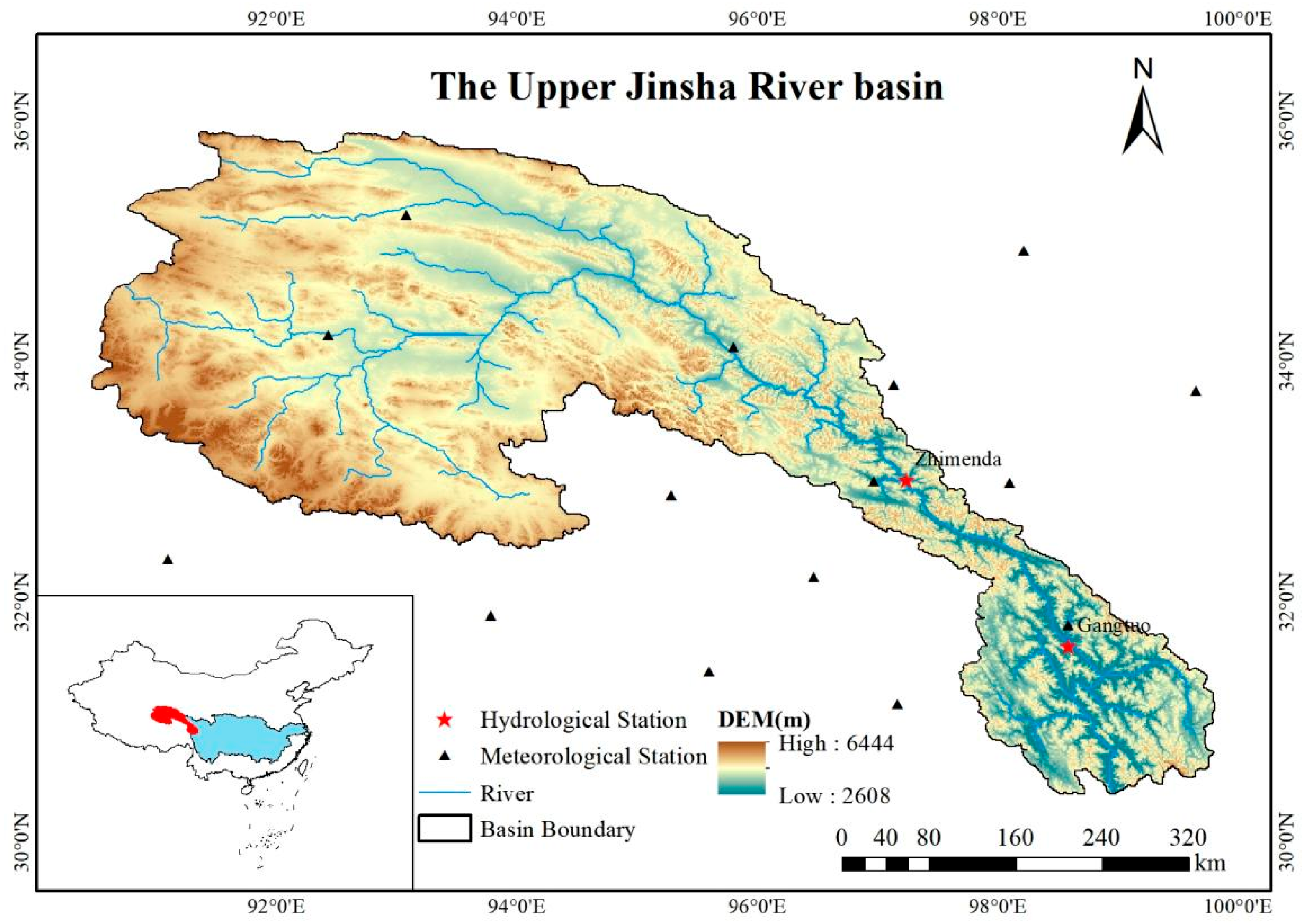As the headwater for over ten major Asian rivers, its role as the “Asian Water Tower” is vital for the water security and socioeconomic development of more than two billion people downstream [2]. The Upper Jinsha River headwaters, known as the “cradle” of the Yangtze River, plays a critical role as its hydrological changes not only serve as a barometer of regional ecological health but also directly influence water allocation and flood control security across the entire Yangtze Basin [3]. Observations show that this region has experienced significant warming in recent decades, with a rate far exceeding the global average. This has triggered profound cryospheric changes, including accelerated glacier retreat, shifts in snow phenology, and thickening of the permafrost active layer. These changes have led to complex alterations in runoff components, flood peak characteristics, and intra-annual flow distribution, which pose unprecedented challenges for runoff simulation and forecasting [4,5,6].

Physically based models (PBMs) have long been the primary tool for studying cryospheric hydrological processes [7,8,9]. Models such as the Variable Infiltration Capacity (VIC) model, the Soil and Water Assessment Tool (SWAT) [10], and the TANK model [11] have been widely applied across the Tibetan Plateau, providing valuable insights into the mechanisms through which climate change affects runoff. These models describe energy and water balances through systems of mathematical–physical equations, providing a solid theoretical foundation. Tshumuka et al. [12] proposed an HBV-Heat model for permafrost-covered regions, which simultaneously accounts for soil physical and thermal properties. This model demonstrated superior performance compared to the standalone HBV model. When driven by reanalysis data such as CMIP6 in the Niang River Basin, the VIC model exhibits significant biases in simulating peak discharge due to systematic underestimation of precipitation intensity and phase errors in complex terrain [13]. A comparative study on daily streamflow prediction based on the coupling of SWAT+ with interpretable machine learning algorithms demonstrated that all four SWAT-ML hybrid models outperformed the standalone SWAT+ model in runoff forecasting [14]. However, their application in high-altitude headwaters faces three major bottlenecks: (1) Inadequate representation of cryospheric processes: Most models use simplified temperature index methods to simulate snow and ice melt, insufficiently capturing complex energy balance processes. Descriptions of soil moisture movement and runoff generation mechanisms under freeze–thaw cycles are often oversimplified, failing to represent the “sponge effect” of permafrost [15]. (2) Substantial uncertainties in input data: Sparse meteorological stations in source regions force a heavy reliance on spatially interpolated, remote sensing, or reanalysis data for model drivers (especially precipitation and air temperature). These datasets, however, contain significant biases over the complex terrain of the plateau [16]. (3) Parameter uncertainty: The complex model structures involve numerous parameters that are difficult to measure directly. The problem of equifinality (different parameter sets yielding similar results) is particularly acute during calibration, which limits simulation accuracy [17]. In this context, the BTOP model was selected as the benchmarking model for this study primarily because its core structure is built upon the TOPMODEL concept, which explicitly links model parameters to topographic indices, its capacity for fine-scale spatial discretization is ideal for our watershed’s complexity, and its integrated snowmelt module is critical for accurately simulating local hydrological processes [18].

Under this backdrop, data-driven models (DDMs), particularly deep learning (DL) [19] methods, have evolved into a powerful alternative for runoff simulation, progressing from early machine learning techniques like multivariate linear regression and ANNs to more advanced recurrent architectures such as RNNs and LSTMs. Li et al. [20] combined K-means clustering with ANNs to improve wave run-up predictions by targeting distinct wave regimes; Liu et al. [21] integrated Time2Vec, Temporal Convolutional Networks, and Transformers to better capture temporal patterns and variable interactions in runoff simulation; Jia et al. [21] developed LightMamba, a lightweight model using a selective state space mechanism, which achieved high-accuracy daily runoff prediction with linear computational complexity, outperforming multiple benchmarks in the Mississippi River Basin. Among these, Long Short-Term Memory (LSTM) networks have become a leading approach, reducing reliance on complex parameterization while integrating multi-source meteorological, surface, and anthropogenic inputs. They excel in capturing temporal dependencies and non-stationarity in hydrological series, with studies by Kratzert et al. [22], Xiang et al. [23], and Feng et al. [24] demonstrating their superior performance and cross-basin generalization capability in large-scale, multi-step, and continental-scale runoff predictions. Building on LSTM, Bidirectional LSTM (BiLSTM) further advances temporal modeling by processing sequences in both forward and backward directions, enabling richer contextual feature extraction and more accurate identification of hydrograph phases—making it theoretically well suited for regions with strong seasonality and complex processes like alpine basins [25]. However, despite its theoretical strengths, BiLSTM remains relatively underutilized in practical runoff simulation and forecasting, particularly in complex and critical basins such as the Jinsha River, where variable climatic influences, intricate topography, and anthropogenic interventions pose modeling challenges that have yet to be fully addressed with bidirectional learning architectures [26].

The Upper Jinsha River Basin is a data-scarce and topographically complex alpine region, and extant research has largely focused on runoff evolution and extreme responses driven by climate change and human activities, along with their attribution. Wang et al. [27] used relative importance analysis to reveal the varying contributions of initial flow, rainfall, and snowmelt to runoff changes across different months. Chen et al. [28] used SWAT model simulations and identified climate change as the dominant factor, with land use change playing a secondary role. Liu et al. [29] applied the rainfall–runoff relation method and the double-mass curve method for attribution, pinpointing the dominant drivers of climate change and human activities in different historical periods. Additionally, Lv et al. [30] investigated the evolving trends in the basin’s hydrological regime under climate and human influences, while Chen and Yang et al. [31] emphasized the importance of model calibration in alpine regions with complex terrain by comparing reanalysis runoff datasets. However, most studies concentrate on macro trends and climate impacts, with a notable scarcity of comparative studies on daily-scale runoff simulation and few explorations aimed at improving short-term forecasting. Given that the Jinsha River constitutes a pivotal water source for the Yangtze river, accurate runoff simulation and flood forecasting are not merely academic exercises but are of paramount importance for downstream water security and flood mitigation for millions of individuals. Consequently, developing robust modeling frameworks capable of precise runoff simulation and short-term forecasting in this complex basin constitutes an urgent scientific and practical importance.

Focusing on the Upper Jinsha River basin, this study conducts a comparative assessment of two modeling paradigms: the distributed, physically based BTOP model and data-driven deep learning architectures (LSTM and BiLSTM). Through a unified framework for runoff simulation and short-term forecasting, we aim to clarify their applicability boundaries and complementary strengths—including the process consistency of physical models versus the forecasting accuracy of data-driven approaches. The results provide a systematic and practical basis for model selection and hydrological forecasting optimization in data-scarce, topographically complex alpine regions.

2. Study Area and Data

2.1. Study Area

The Jinsha River originates in the plateau region, spanning Qinghai Province, the Tibet Autonomous Region, Sichuan, and Yunnan Province. It is an important part of the Upper Yangtze River. The section above the Zhimenda Station is considered the source region of the Yangtze River. The main river channel stretches approximately 1120 km from this source to Zhimenda Station and extends another 283 km downstream to Gangtuo Station. The catchment areas controlled by Zhimenda and Gangtuo Stations are 157,000 km² and 161,000 km², respectively. This study focuses on the Jinsha River upstream of Gangtuo Station, shown in Figure 1. The region is characterized by rugged topography and deeply incised valleys, forming a typical alpine–gorge landscape. The basin exhibits a typical plateau climate with distinct vertical zonation. The mean annual temperature decreases markedly with increasing elevation, ranging from −4.8 °C to 14.82 °C, while average annual precipitation varies spatially from approximately 228 mm to 953 mm, generally increasing from the northwest to the southeast [32]. Its hydrology is dominated by the monsoon, with approximately 70% of the annual precipitation concentrated from June to September. This results in a strongly seasonal regime with high flows in summer and low flows in winter [33]. As an alpine region, the basin’s runoff is driven by multiple processes: glacial melt, snowmelt, seasonal frozen ground dynamics, and rainfall. The contribution of these components exhibits significant interannual and intra-annual variations, governed by their spatiotemporal distribution, climatic conditions, and cryospheric evolution [34,35]. Consequently, river runoff is primarily supplied by precipitation and meltwater from glaciers and seasonal snowpack.

The Upper Jinsha River is a key headwater region of the Yangtze River, and its runoff regime critically influences downstream hydrology and water resource management. Accurate runoff simulation and short-term forecasting are therefore crucial for anticipating the timing and magnitude of flood peaks, thus supporting scientific reservoir operation and downstream early warning systems for floods.

2.2. Data

This study utilized meteorological data, hydrological data, land surface characteristic data, and other ancillary datasets.

The hydrological data consist of daily discharge records (2006–2022) from the Zhimenda and Gangtuo Stations, which were obtained from the Hydrological Bureau of the Yangtze River Water Resources Commission. Meteorological data were obtained from relevant meteorological departments and the National Meteorological Science Data Centre website. The study area and its surrounding region comprise a total of 15 meteorological stations. This corresponds to a station density of approximately 1.6 stations per 100,000 km², emphasizing the severe scarcity of ground-based observational data in this critical headwater region [36]. The Digital Elevation Model (DEM) is derived from the high-precision MERIT-DEM (Multi-Error-Removed Improved-Terrain DEM) product, featuring a global resolution of 3 arcseconds. Soil data were sourced from the Food and Agriculture Organization (FAO). Land use data were sourced from the Copernicus Global Land Service. Evapotranspiration data (ET) and leaf area index (LAI) data were sourced from ERA5-Land reanalysis products.

The multi-source data collected have undergone unified quality control and normalization processing to ensure data consistency and reliability.

3. Methodology

3.1. BTOP Model

The BTOP (Block-wise use of TOPMODEL with Muskingum–Cunge routing) model [37] is a distributed, physically based model that simulates runoff generation and flow routing based on topographic index concepts. It is designed to represent the complete rainfall–runoff process within a river network. The model partitions a catchment into multiple blocks or sub-regions using a DEM and information on terrain, soil, and vegetation. It integrates the Muskingum–Cunge method to simulate channel flow, thereby enabling accurate simulation of the spatiotemporal evolution of flood waves. The physical model’s snowmelt module and scalability enable adaptation to diverse climatic conditions and geographical environments for robust hydrological simulation. The BTOP model offers the following significant advantages: (1) Parameter Regionalization: The model’s block-wise structure links key hydrological parameters to underlying topography, soil, and vegetation characteristics. Parameters are calibrated within each block, which reduces the heavy reliance on empirical calibration common in traditional distributed models and maintains a consistent parameter set. This lowers the model’s degrees of freedom and computational cost, making it suitable for larger regions or applications at medium resolutions [18]. (2) Physical Interpretability: The BTOP model requires the calibration of relatively few parameters, each with a clear physical meaning. This facilitates the analysis of how different land surfaces and climatic conditions influence hydrological responses. (3) Snow and Ice Melt Module: The model uses a degree-day method to simulate snowmelt and ice melt runoff, which has few parameters and is computationally straightforward, making it widely applicable in data-scarce regions. A summary of the key parameters calibrated for the BTOP model is provided in

Table 1. Parameters to be determined for BTOP model.

Parameters	Unit	Physical Significance	Value Range
D0clay	m/Δt	Groundwater discharge capacity for (clay/loam/silt) soil textures clay, loam, silt	[0.01, 2]
D0sand			[0.01, 2]
D0silt			[0.01, 2]
SDbar	m	Mean unsaturated zone storage deficit	[0.001, 0.9]
m	m	Flow recession coefficient	[0.01, 0.1]
n0	s/m1/3	Manning’s roughness coefficient	[0.00001, 0.8]
α	/	Drying coefficient	[−10, 10]

.

3.2. LSTM Model

The Long Short-Term Memory (LSTM) model, proposed by Hochreiter and Schmidhuber [38], is based on the design of gated memory units (input gate, forget gate, output gate) and an error feedback channel. Without requiring the explicit construction of complex rule mechanisms and parameter systems, it can automatically learn cross-time-lag nonlinear mappings from data, significantly alleviating the vanishing gradient problem inherent in traditional recurrent neural networks.

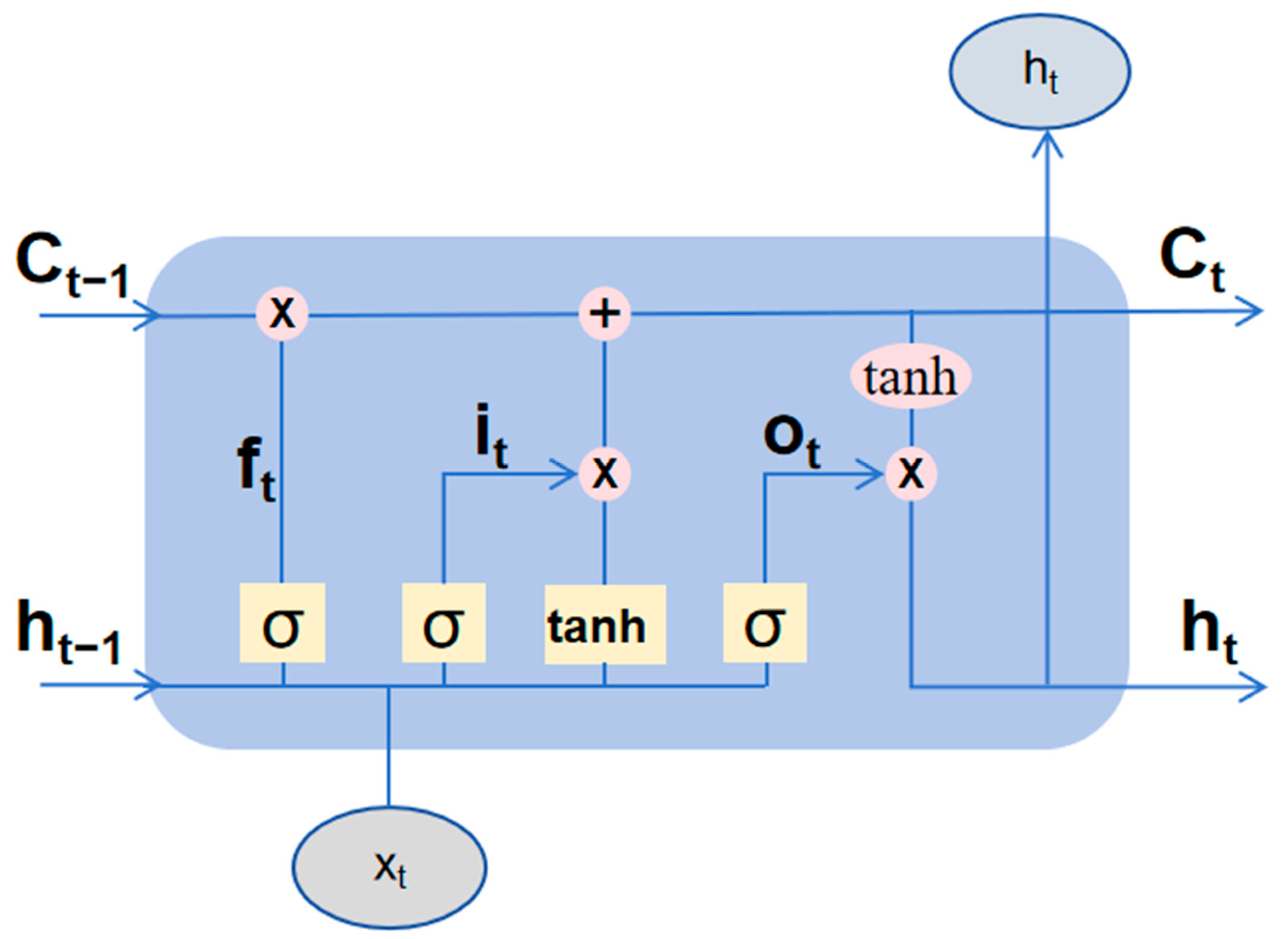
LSTM neural networks enhance their long-term memory capabilities by introducing control units such as the forget gate (${\mathrm{f}}_{\mathrm{t}}$), input gate (${\mathrm{i}}_{\mathrm{t}}$) and output gate (${\mathrm{o}}_{\mathrm{t}}$) which maintain and update the cell state [39]. Figure 2 depicts an LSTM network model featuring three gated structures.

The module contains the cell state storing information and three control gates governing information flow. The input gate determines which information from the potential cell state is permitted to pass through to update the current cell state. The forget gate governs which information from the previous cell state C_t−1 is retained or discarded; finally, the output gate controls which information from the current cell state may flow into the new hidden cell state h_t+1. This three-gate structure regulates the flow and preservation of information within the cell unit state [40].

The forget gate determines which information from the previous time step’s cell state (C_t−1) requires discarding. At each time step, the gates are updated by the following equations:

$${\mathrm{f}}_{\mathrm{t}}=\mathsf{\sigma }\left({\mathrm{W}}_{\mathrm{f}}{\mathrm{x}}_{\mathrm{t}}+{\mathrm{U}}_{\mathrm{f}}{\mathrm{h}}_{\mathrm{t}-1}+{\mathrm{b}}_{\mathrm{f}}\right)$$

(1)

$${\tilde{\mathrm{c}}}_{\mathrm{t}}=\tanh \left({\mathrm{W}}_{\mathrm{c}}{\mathrm{x}}_{\mathrm{t}}+{\mathrm{U}}_{\mathrm{c}}{\mathrm{h}}_{\mathrm{t}-1}+{\mathrm{b}}_{\mathrm{c}}\right)$$

(2)

$${\mathrm{i}}_{\mathrm{t}}=\mathsf{\sigma }\left({\mathrm{W}}_{\mathrm{i}}{\mathrm{x}}_{\mathrm{t}}+{\mathrm{U}}_{\mathrm{i}}{\mathrm{h}}_{\mathrm{t}-1}+{\mathrm{b}}_{\mathrm{i}}\right)$$

(3)

$${\mathrm{C}}_{\mathrm{t}}={\mathrm{f}}_{\mathrm{t}}\odot {\mathrm{C}}_{\mathrm{t}-1}+{\mathrm{i}}_{\mathrm{t}}\odot {\tilde{\mathrm{c}}}_{\mathrm{t}}$$

(4)

$${\mathrm{o}}_{\mathrm{t}}=\mathsf{\sigma }\left({\mathrm{W}}_{\mathrm{o}}{\mathrm{x}}_{\mathrm{t}}+{\mathrm{U}}_{\mathrm{o}}{\mathrm{h}}_{\mathrm{t}-1}+{\mathrm{b}}_{\mathrm{o}}\right)$$

(5)

$${\mathrm{h}}_{\mathrm{t}}={\mathrm{o}}_{\mathrm{t}}\odot \tanh ({\mathrm{C}}_{\mathrm{t}})$$

(6)

${\mathrm{x}}_{\mathrm{t}}$ is the input vector at time step t, ${\mathrm{h}}_{\mathrm{t}}$ is the hidden state at time step t, ${\mathrm{C}}_{\mathrm{t}}$ is the cell state at time step t, and ${\tilde{\mathrm{c}}}_{\mathrm{t}}$ represents the candidate cell state. The symbols ${\mathrm{f}}_{\mathrm{t}}$, ${\mathrm{i}}_{\mathrm{t}}$, and ${\mathrm{o}}_{\mathrm{t}}$ denote the forget gate, input gate, and output gate, respectively. $\mathrm{W}$ and U are the weight matrices, while b denotes the bias term. $\mathrm{\sigma }$ is a Sigmoid function, and $\tan \mathrm{h}$ is the hyperbolic tangent function. $\odot$ is the element-wise multiplication (Hadamard product).

3.3. BiLSTM Model

BiLSTM is a further extension of LSTM. [41]. Unlike unidirectional LSTMs which rely solely on historical information, BiLSTMs incorporate a reverse-processed LSTM layer to simultaneously utilize both past and future contextual information within a sequence. This enables a more comprehensive capture of bidirectional dependencies within the sequence. This bidirectional propagation structure endows BiLSTMs with greater expressive power in time-series modeling, particularly in capturing complex temporal dependencies. 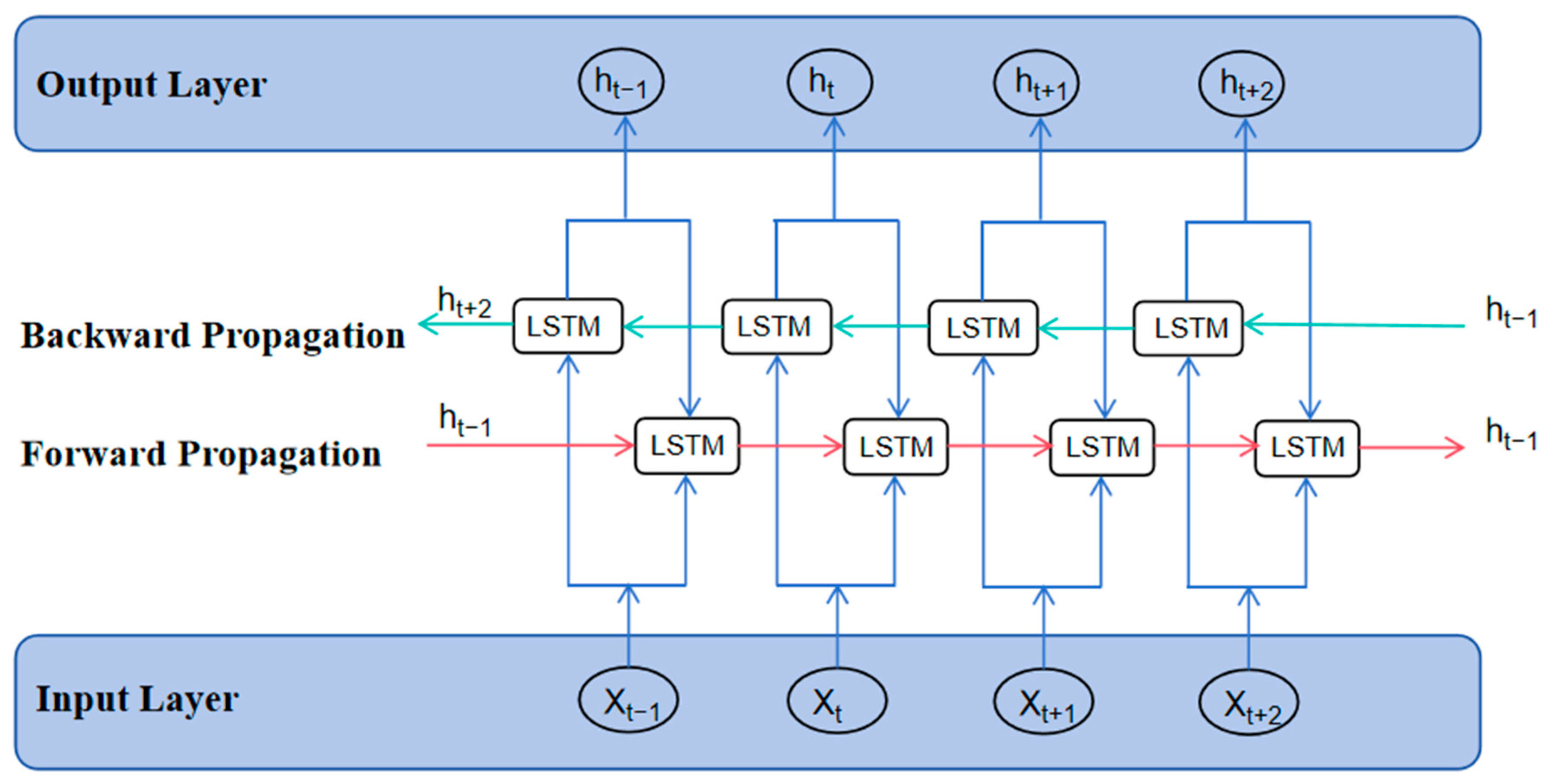Compared to unidirectional LSTMs, BiLSTMs demonstrate superior accuracy [42]. The BiLSTM network architecture is illustrated in Figure 3, comprising three principal components: the input layer, the bidirectional LSTM layer, and the output layer [43]. At the input layer, the input vector for each time step is denoted as xt. BiLSTM simultaneously performs forward (past → future) and backward (future → past) information propagation and state updates on the time series, thereby capturing the bidirectional dependencies within the sequence more comprehensively. The forward LSTM handles the forward dependencies of the input sequence, while the backward LSTM captures the reverse dependencies. The bidirectional output at each time step is jointly determined by the hidden states of both the forward and backward LSTMs, as depicted in the calculation process shown in the equations below.

$$\overrightarrow{{\mathrm{h}}_{\mathrm{t}}}=\mathrm{L}\mathrm{S}\mathrm{T}\mathrm{M}({\mathrm{x}}_{\mathrm{t}},\overrightarrow{{\mathrm{h}}_{\mathrm{t}-1}})$$

(7)

$$\overleftarrow{{\mathrm{h}}_{\mathrm{t}}}=\mathrm{L}\mathrm{S}\mathrm{T}\mathrm{M}({\mathrm{x}}_{\mathrm{t}},\overleftarrow{{\mathrm{h}}_{\mathrm{t}-1}})$$

(8)

$${\mathrm{h}}_{\mathrm{t}}={\mathsf{\omega }}_{\mathrm{t}}\overrightarrow{{\mathrm{h}}_{\mathrm{t}}}+{\mathrm{v}}_{\mathrm{t}}\overleftarrow{{\mathrm{h}}_{\mathrm{t}}}+{\mathrm{b}}_{\mathrm{t}}$$

(9)

${\mathrm{x}}_{\mathrm{t}}$ is the input feature vector for the t-th time step; $\overrightarrow{{\mathrm{h}}_{\mathrm{t}}}$ is the hidden state of the forward LSTM at time step t, calculated by the current input ${\mathrm{x}}_{\mathrm{t}}$ and the previous forward hidden state $\overrightarrow{{\mathrm{h}}_{\mathrm{t}-1}}$. $\overleftarrow{{\mathrm{h}}_{\mathrm{t}}}$ is the hidden state of the reverse LSTM at time step t. It is calculated by the current input ${\mathrm{x}}_{\mathrm{t}}$ and the reverse hidden state $\overleftarrow{{\mathrm{h}}_{\mathrm{t}-1}}$ at the next moment. ${\mathrm{h}}_{\mathrm{t}}$ is the final output state of the BiLSTM, obtained by weighting and summing the forward and backward hidden states, then adding the bias term. ${\mathsf{\omega }}_{\mathrm{t}}$ and ${\mathrm{v}}_{\mathrm{t}}$ are the weighting parameters for the forward and reverse hidden states, respectively, serving to balance the contribution of bidirectional information. ${\mathrm{b}}_{\mathrm{t}}$ enhances the model’s ability to represent nonlinear relationships.

3.4. Experimental Design and Parameter Configuration

In this study, we first used the collected dataset to construct three distinct models: the physics-based BTOP model, and the data-driven LSTM and BiLSTM models. Model parameters were optimized accordingly: the BTOP model’s parameters were calibrated using the SCE-UA algorithm, while the optimal architectures and hyperparameters for the LSTM and BiLSTM models were identified via tuning and validation on a separate dataset. Subsequently, all three models were used to conduct runoff simulations, and their results were compared to evaluate their respective applicability for short-term forecasting within the study area. Finally, multi-step short-term forecasting was performed using the LSTM and BiLSTM models for forecast periods of 1 d, 3 d, 5 d, and 7 d to systematically analyze their forecasting capabilities and error propagation characteristics at different horizons.

The flowchart of this study is shown in Figure 4.

3.4.1. Dataset Partitioning and Preprocessing

The BTOP model was calibrated from 2006 to 2017 and tested from 2018 to 2022. To ensure a fair comparison, the LSTM and BiLSTM models followed a consistent data partitioning scheme: the period from 2006 to 2015 was used for training, 2016 to 2017 for validation and hyperparameter tuning, and 2018 to 2022 for testing. This alignment ensures that the combined training and validation phases of the machine learning models correspond to the calibration period of the BTOP model, thereby guaranteeing that all models are evaluated on a common test period. All data were subjected to quality control. For the deep learning models, both the input features and the target runoff series were standardized using Z-scores. Furthermore, all comparative experiments followed a consistent data processing workflow, model configuration protocol, and evaluation criteria to ensure the objectivity and reproducibility of the results.

3.4.2. Model Architecture and Training Configuration

LSTM and BiLSTM comprise two stacked layers of recurrent neural networks. The first layer is configured with ‘return_sequences = True’ to enhance the models’ ability to extract temporal sequence information. Each recurrent layer is followed by a LeakyReLU activation function, with L2 regularization (λ = 0.01) applied to prevent overfitting. Finally, a fully connected layer (Dense) outputs the one-step ahead flow prediction result. Training configuration: Both models share identical training hyperparameters. The optimizer is Adam with a fixed learning rate (α) of 0.002. The loss function is Mean Squared Error (MSE). The model training batch size (batch_size) was set to 64, with a total of 100 training epochs. The time window length (Window Size) was 60, and the number of hidden layer units (Hidden Layer Units) was 60 [43]. All experiments were conducted in a GPU-accelerated environment with memory allocated on demand.

The distinction between the two models lies in the direction of the recurrent layers: the LSTM model employs a standard unidirectional LSTM architecture, whereas the BiLSTM model replaces both recurrent layers with bidirectional LSTMs to simultaneously extract both forward and backward dependencies within the time series.

3.4.3. Experimental Scenario

(1)

Runoff Simulation Scenario

This scenario aims to investigate model performance in daily-scale runoff simulation and to evaluate its applicability for forecasting in alpine regions. After preprocessing, the data were fed into the BTOP, LSTM, and BiLSTM models. The BTOP model was calibrated for optimal parameters, while the deep learning models were optimized (architecture and hyperparameters) using a validation set. All models were ultimately evaluated on a held-out test set.

(2)

Short-Term Forecasting Scenario

This experimental scenario serves to evaluate the forecasting accuracy of the LSTM model across different forecast periods. The target length is set as target size = {1, 3, 5, 7}, corresponding to 1 d, 3 d, 5 d, and 7 d runoff forecasts, respectively. For each forecast period, an independent supervised learning model is constructed and trained to ensure that each model possesses targeted predictive capability and stability at its respective timescale.

In the aforementioned two types of scenario experiments, the LSTM model refers to LSTM and BiLSTM.

3.5. Model Accuracy Evaluation Metrics

Numerous studies have employed the Nash efficiency coefficient (NSE) [44], Kling–Gupta efficiency coefficient (KGE) [45], root mean square error (RMSE) [45], and relative bias (RBIAS) [46] to assess the accuracy of runoff simulation/prediction. The formulas are as follows:

(1)

Nash Efficiency

The Normalized Sum of Squares Error (NSE) serves as the most commonly employed efficiency metric for hydrological models. Its range extends from negative infinity to 1, with values closer to 1 indicating superior simulation performance. Generally, an NSE exceeding 0.5 is regarded as indicative of a model’s high reliability. The NSE is defined as follows:

$$\mathrm{N}\mathrm{S}\mathrm{E}=1-{\displaystyle \frac{\sum _{\mathrm{i}=1}^{\mathrm{n}}({\mathrm{Q}}_{\mathrm{s}\mathrm{i}\mathrm{m},\mathrm{i}}-{\mathrm{Q}}_{\mathrm{o}\mathrm{b}\mathrm{s},\mathrm{i}}{)}^2}{\sum _{\mathrm{i}=1}^{\mathrm{n}}({\mathrm{Q}}_{\mathrm{o}\mathrm{b}\mathrm{s},\mathrm{i}}-{\overline{\mathrm{Q}}}_{\mathrm{o}\mathrm{b}\mathrm{s}}{)}^2}}$$

(10)

where $\mathrm{n}$ is the total number of time steps; ${\mathrm{Q}}_{\mathrm{obs},\mathrm{i}}$ and ${\mathrm{Q}}_{\mathrm{sim},\mathrm{i}}$ are the observed and simulated river discharge at time step $\mathrm{i}$, and the mean values are denoted as ${\mathrm{Q}}_{\mathrm{obs}}$ and Q_sim.

(2)

Kling–Gupta Efficiency Coefficient

KGE is more sensitive to variance and high flow rates, with values in the range of ∞→1. Generally, the closer the KGE value is to 1, the better the fitting effect. KGE is defined as follows:

$$\mathrm{KGE}=1-\sqrt{(\mathrm{r}-1{)}^2+(\mathrm{\beta }-1{)}^2+(\mathrm{\gamma }-1{)}^2}$$

(11)

r is the Pearson’s correlation coefficient, β is the bias ration, and γ is the variability ration.

(3)

Root Mean Square Error

Root Mean Square Error (RMSE) reflects the average scale of error, defined as the square root of the mean of the squared differences between observations and simulations. Its units are consistent with the measured variable (in this study, m³/s), with values in the range of [0, +∞). A lower value is preferable.

$$\mathrm{R}\mathrm{M}\mathrm{S}\mathrm{E}=\sqrt{{\displaystyle \frac{1}{\mathrm{n}}}\sum _{\mathrm{i}=1}^{\mathrm{n}}({\mathrm{Q}}_{\mathrm{s}\mathrm{i}\mathrm{m},\mathrm{i}}-{\mathrm{Q}}_{\mathrm{o}\mathrm{b}\mathrm{s},\mathrm{i}}{)}^2}$$

(12)

(4)

Relative BIAS

The average deviation of model predictions relative to observed values serves as a measure of model accuracy. A positive value indicates that model predictions are generally higher than observed values, while a negative value indicates that model predictions are generally lower than observed values.

$$\mathrm{R}\mathrm{B}\mathrm{I}\mathrm{A}\mathrm{S}\left(\mathrm{\%}\right)={\displaystyle \frac{\sum _{\mathrm{i}=1}^{\mathrm{n}}({\mathrm{Q}}_{\mathrm{s}\mathrm{i}\mathrm{m},\mathrm{i}}-{\mathrm{Q}}_{\mathrm{o}\mathrm{b}\mathrm{s},\mathrm{i}})}{\sum _{\mathrm{i}=1}^{\mathrm{n}}{\mathrm{Q}}_{\mathrm{o}\mathrm{b}\mathrm{s},\mathrm{i}}}}\times 100\mathrm{\%}$$

(13)

4. Results

4.1. Runoff Simulation Results

4.1.1. BTOP Daily-Scale Runoff Simulation Results

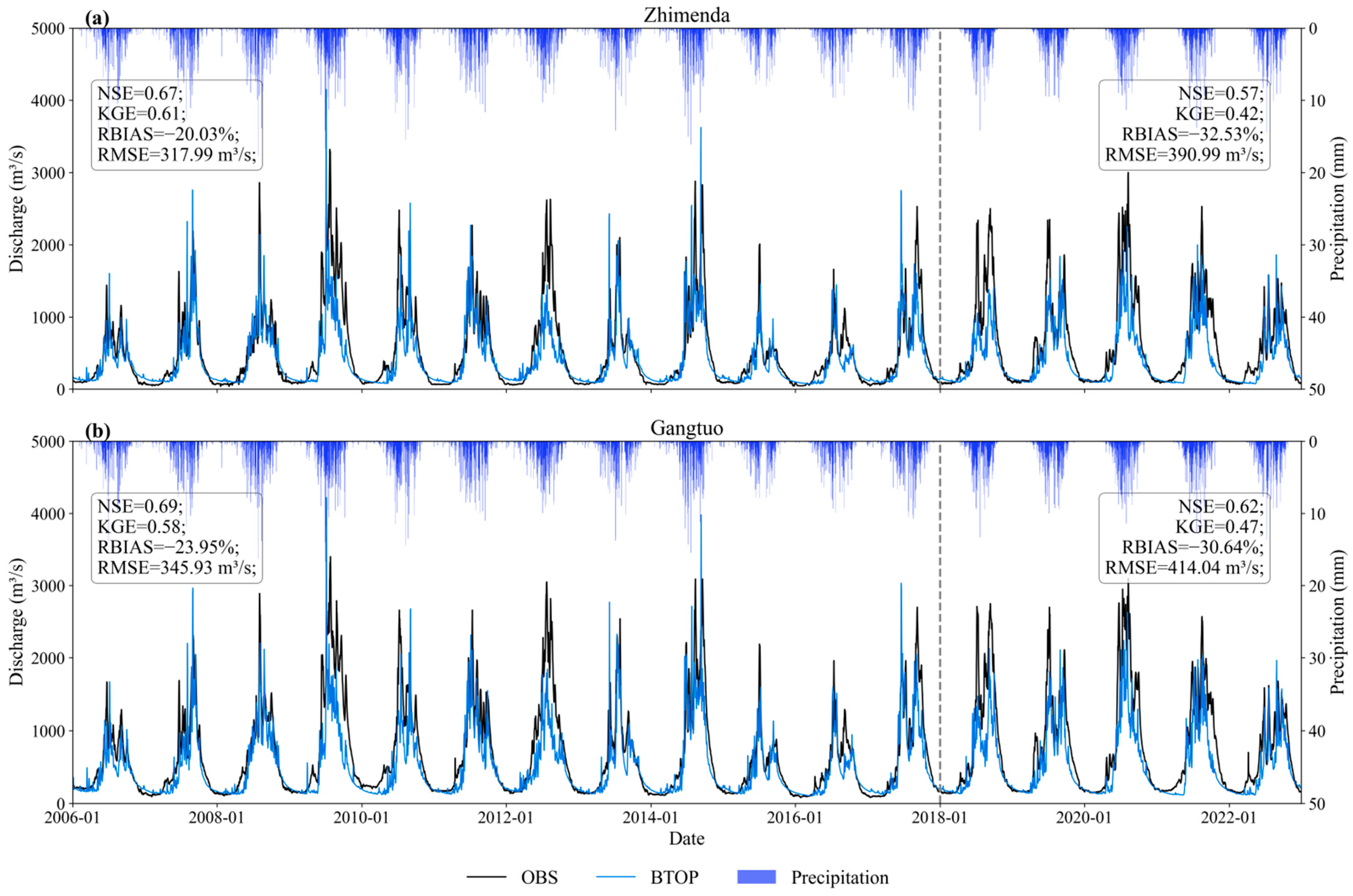
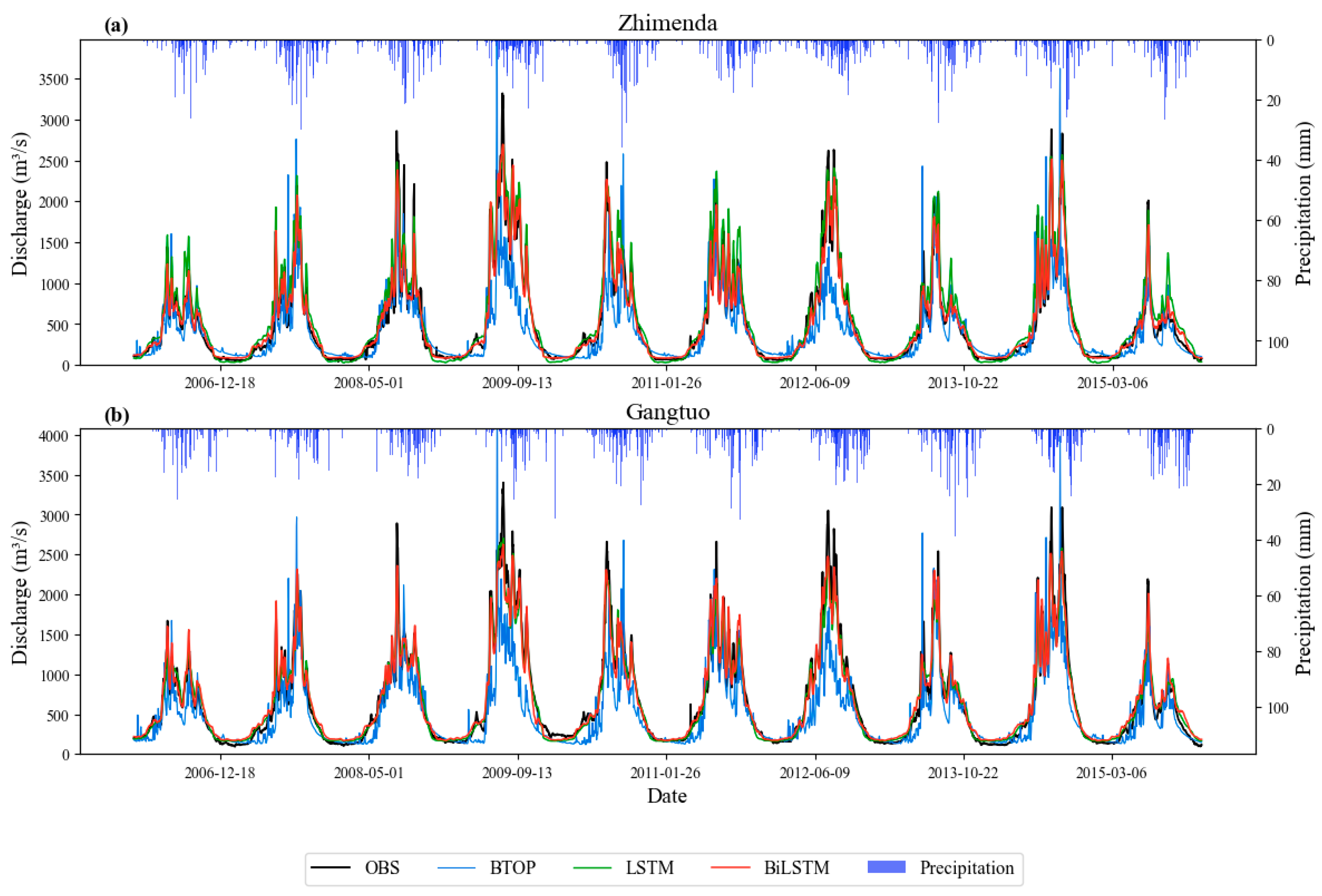
The daily runoff simulations from the BTOP model are shown in Figure 5. Overall, the model captures the general trends of the observed hydrographs at both Gangtuo and Zhimenda Stations. It reproduces key characteristics, including the timing of flood season peaks, interannual variability, and typical seasonal patterns such as the rapid rise in flow during late spring and early summer.

The model performs stably during low-flow periods, with simulated recession curves aligning well with observations. However, it shows systematic deviations in reproducing specific events, primarily an underestimation of peak flows (e.g., in 2012, 2018, and 2020) and occasional overestimation (e.g., in 2007 and 2009). These discrepancies likely arise from sparse station coverage and the limited representativeness of meteorological data in high-altitude regions, combined with the model’s inadequate representation of key runoff generation mechanisms, such as the spatiotemporal heterogeneity of precipitation, snowmelt dynamics, and seasonal frozen soil processes.

The daily-scale runoff simulation metrics for the BTOP model are presented in

Table 2. Runoff simulation results.

Station	Period	Model	NSE	KGE	RBIAS (%)	RMSE (m3/s)
Zhimenda	Training	BTOP	0.67	0.61	−20.03	317.99
		LSTM	0.93	0.79	13.61	151.13
		BiLSTM	0.97	0.95	0.68	89.35
	Test	BTOP	0.57	0.42	−32.53	390.99
		LSTM	0.82	0.91	2.72	252.33
		BiLSTM	0.81	0.80	−11.80	261.76
Gangtuo	Training	BTOP	0.69	0.58	−23.95	345.93
		LSTM	0.96	0.90	−1.44	118.72
		BiLSTM	0.96	0.91	1.31	117.74
	Test	BTOP	0.62	0.47	−30.64	414.04
		LSTM	0.87	0.91	−3.66	244.91
		BiLSTM	0.86	0.91	−2.74	250.62

. At Zhimenda Station, the NSE and KGE declined from 0.67 and 0.61 in the calibration period to 0.57 and 0.42 in the validation period, respectively. Concurrently, the RMSE rose from 317.99 m³/s to 390.99 m³/s, and the RBIAS shifted from −20.03% to −32.53%, collectively indicating a significant and worsening systematic underestimation. In contrast, performance metrics at Gangtuo Station were more stable between the calibration and validation periods, despite substantial overall bias. The RMSE values at Gangtuo (330.86 m³/s for calibration; 407.24 m³/s for validation) were higher than those at Zhimenda. This is expected, as Gangtuo is located downstream and experiences higher flow magnitudes. During validation, Gangtuo’s NSE and KGE also declined to 0.62 and 0.47, respectively, with an RBIAS of −30.64%. This performance degradation in the validation period underscores the complexity of hydrological processes in alpine regions and points to limitations in both the model’s input drivers and its parameterization. In summary, the BTOP model effectively captures the broad interannual and seasonal patterns of runoff and shows reasonable skill in simulating the timing of summer floods and winter low flows. However, it consistently underestimates peak flow magnitudes, indicating a structural or parametric limitation in representing high-flow dynamics and highlighting a key area for future model improvement.

4.1.2. LSTM Daily-Scale Runoff Simulation Results

The LSTM model’s test period runoff simulations are shown in Figure 6. The model effectively captures the overall hydrograph and represents the magnitude of certain flood peaks more closely to observations than the BTOP model does. Although it accurately captures many peaks, its performance is inconsistent, with overestimation in some years (e.g., 2011) and underestimation in others (e.g., 2014). A notable issue is the model’s general underestimation of low-flow discharges at Zhimenda Station, which may be attributed to its limited ability to represent the contribution of snowmelt recharge processes.

Evaluation metrics for the LSTM model’s daily-scale runoff simulations are presented in Table 2, showing substantial improvement over the BTOP model across all indicators. During the training period, the LSTM model showed dramatic improvements over BTOP: NSE rose by 0.27 to 0.96, KGE by 0.32 to 0.90, RMSE decreased by 65.7% to 118.72 m³/s, and RBIAS was substantially reduced to −1.44%. Superior performance persisted in the test period, with the NSE being 0.25 higher (0.87), KGE being 0.44 higher (0.91), RMSE being 40.8% lower (244.91 m³/s), and RBIAS sharply improving (−3.66%), representing an 88.1% reduction in bias magnitude compared to BTOP. These results demonstrate that the LSTM model significantly outperforms the physical model in accuracy, error control, and bias correction, demonstrating its strong potential for runoff simulation in such complex environments.

4.1.3. BiLSTM Simulation Results

The BiLSTM model’s runoff simulations during the test period are presented in Figure 6. The model captures the overall hydrograph well and demonstrates slightly superior performance to the LSTM in simulating certain peak flows and capturing runoff dynamics during specific periods. Although performance varies across flood events, and the simulation accuracy for peaks and recession limbs of some small-to-medium events remains slightly inadequate, its overall performance is stable.

The evaluation metrics in Table 2 and Figure 7 confirm the outstanding performance of the BiLSTM model in daily runoff simulation, with all metrics significantly surpassing those of the BTOP model. At Zhimenda Station, for instance, the BiLSTM achieved an NSE of 0.97 during the training period—0.30 higher than BTOP’s 0.67—and reduced the RMSE by 71.9% to 89.35 m³/s. During test period, its KGE of 0.80 was 0.38 higher than BTOP’s 0.42, indicating a better representation of hydrological processes. An analysis of the RBIAS metric reveals a pronounced negative bias in the BTOP model at both stations and across all periods. During the training period, biases were −20.83% at Zhimenda and −23.35% at Gangtuo, which further widened during test period, confirming a persistent systematic underestimation.

A detailed analysis of the LSTM model at Zhimenda Station reveals a distinct pattern. As shown in Table 2, during the training period, BiLSTM’s bidirectional architecture demonstrated a clear advantage for data fitting, achieving superior metrics (NSE: 0.97 vs. 0.93; RMSE: 89.35 vs. 151.13 m³/s; RBIAS: 0.68% vs. 13.61%). However, this advantage diminished during the test period. While the NSE values were comparable (0.81 vs. 0.82), BiLSTM exhibited a lower KGE (0.80 vs. 0.91) and a higher systematic bias (RBIAS: −11.80% vs. 2.72%). This trend is further supported by the greater decline in NSE from the training to test period for BiLSTM (e.g., −0.16 at Zhimenda vs. LSTM’s −0.11), suggesting that the bidirectional architecture has a tendency toward overfitting, where the model’s complexity may have led to memorization of training data at the expense of robust generalization.

Unlike the physical model, the LSTM and BiLSTM models show significantly lower and more stable biases. Their predictions maintain low biases (consistently within ±13%) across both calibration and validation periods at all stations, effectively correcting the systematic underestimation inherent in the physical model.

4.1.4. Flood Event Comparison Results

To further evaluate the capacity of different models to capture and characterize flood peaks, a comparative analysis was conducted using representative flood events of different magnitudes from the study period. Flood events were classified into four categories based on their peak discharge: extreme floods: 3000–4000 m³/s; major floods: 2500–3000 m³/s; medium floods: 2000–2500 m³/s; minor floods: 1500–2000 m³/s.

Given the high similarity in runoff processes between the Zhimenda and Gangtuo Stations, the analysis focused on Gangtuo Station. Representative floods from each category were selected, and their hydrographs were plotted to compare model performance across events and magnitudes.

The simulation results for these typical flood events (Figure 8) reveal marked differences in the models’ abilities to reproduce flood hydrographs at Gangtuo Station.

Event 1 (Flood Peak 3000–4000 m³/s), as shown in Figure 8a: The BTOP model severely misrepresented both the magnitude and timing of the peak. In contrast, both LSTM and BiLSTM models effectively captured the overall flood process, including the timing of the main peak and the characteristics of preceding smaller peaks, although they significantly underestimated the ultimate peak magnitude.

Event 2 (Flood Peak 2500–3000 m³/s), as shown in Figure 8b: BTOP significantly underestimated the peak and showed a slow response. LSTM and BiLSTM more accurately simulated the rising limb and provided better peak estimates, with BiLSTM slightly outperforming LSTM in peak magnitude. However, both deep learning models exhibited an overly rapid recession.

Event 3 (Flood Peak 2000–2500 m³/s), as shown in Figure 8c: For the first peak in this event, BTOP accurately estimated the magnitude but with early timing. BiLSTM accurately simulated both the timing and magnitude, while LSTM captured the timing correctly but produced the poorest magnitude estimate. For the second peak, all models captured the trend but significantly underestimated the magnitude, likely due to unrepresentative precipitation inputs. Despite this, LSTM and BiLSTM better captured the timing and the overall rising and falling pattern.

Event 4 (Flood Peak 1500–2000 m³/s), as shown in Figure 8d: BTOP showed a rapid rise, significant peak underestimation, and a slow response. Both LSTM and BiLSTM provided a reasonable fit, with BiLSTM significantly outperforming LSTM in peak estimation, though both deviated during the recession.

In summary, the LSTM and BiLSTM models demonstrated a robust ability to reproduce the shape of the flood hydrograph across most events and magnitudes, showing strong skill in identifying peak timing. BiLSTM held a slight overall edge over LSTM in simulating peak magnitudes, underscoring the advantage of its bidirectional structure in capturing temporal dependencies. In contrast, the BTOP model showed inconsistent performance, with timing errors (early or delayed peaks) and variable accuracy in peak magnitude, reflecting the limitations of traditional hydrological models in complex terrains.

A key limitation for both deep learning models was their tendency to simulate an overly rapid recession, indicating room for improvement in low-flow mechanism representation. Furthermore, the systematic underestimation of the most extreme peaks suggests potential issues with input data representativity. Nevertheless, the consistent ability of the LSTM and BiLSTM models to accurately identify the timing of flood peaks and capture the overall process dynamics underscores their significant practical value for flood early warning and forecasting operations in the study region.

4.2. Short-Term Forecasting Results

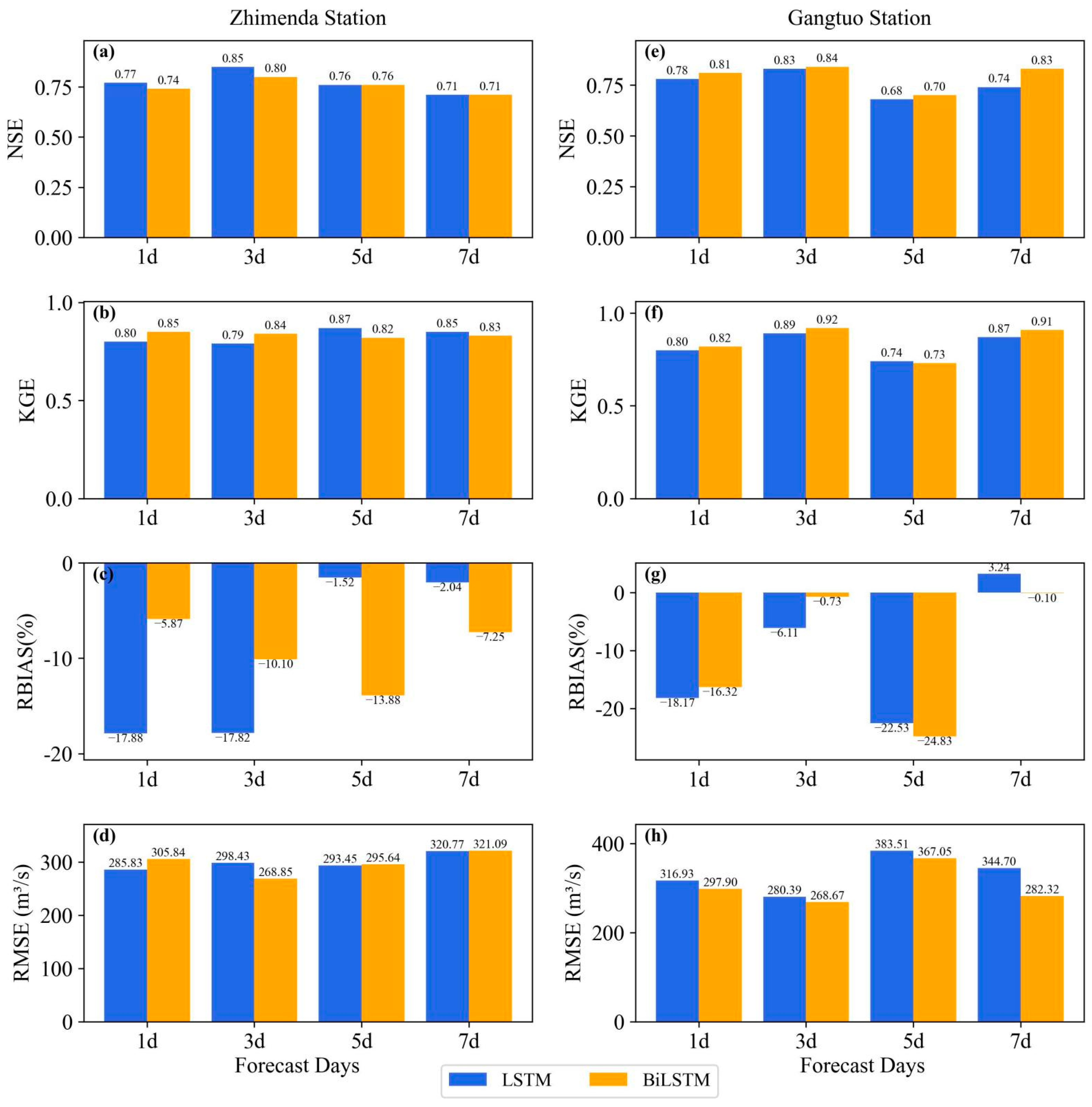
The short-term forecasting results are presented in Figure 9. Overall, the performance of the two models is comparable, while their relative strengths vary by station and forecast period.

At Zhimenda Station, the LSTM model showed satisfactory performance for short forecast periods (1–3 d), with NSE values ranging from 0.77 to 0.85 and KGE values ranging from 0.79 to 0.87. However, its accuracy diminished at the 7 d forecast period (NSE = 0.71, RMSE = 320.77 m³/s). BiLSTM achieved marginally higher KGE values (0.84–0.85) but slightly lower NSE and higher RMSE values than LSTM over 1–3 d, indicating largely comparable performance between the two models at this station.

At Gangtuo Station, a different pattern emerged. The LSTM model performed best at the 3 d forecast period (NSE = 0.83, KGE = 0.89) but suffered a marked decline at 5 d (NSE = 0.68, RBIAS = −22.53%). In contrast, BiLSTM demonstrated greater robustness, maintaining high accuracy (NSE = 0.83, KGE = 0.91, RBIAS ≈ 0) even at the 7 d forecast period. This highlights BiLSTM’s superior capability for longer-term forecasts at Gangtuo.

The comparative analysis reveals distinct model strengths:

BiLSTM excels at Gangtuo Station, particularly for 3–7-day forecasts, outperforming LSTM in NSE, KGE, and bias control, demonstrating greater robustness.

LSTM holds a slight edge at Zhimenda Station for 1–3-day forecasts, generally achieving a marginally higher NSE.

A common issue across both models is the systematic underestimation, indicated by predominantly negative RBIAS values, with the most severe case being LSTM’s 5 d forecast at Gangtuo Station (−22.53%). Furthermore, model errors do not increase monotonically with forecast period. For instance, at Gangtuo Station, accuracy was higher at 3 d and 7 d forecast periods than at 5 d. This non-monotonic error progression underscores the complex nature of error propagation and suggests that model performance is influenced by factors beyond the forecast horizon.

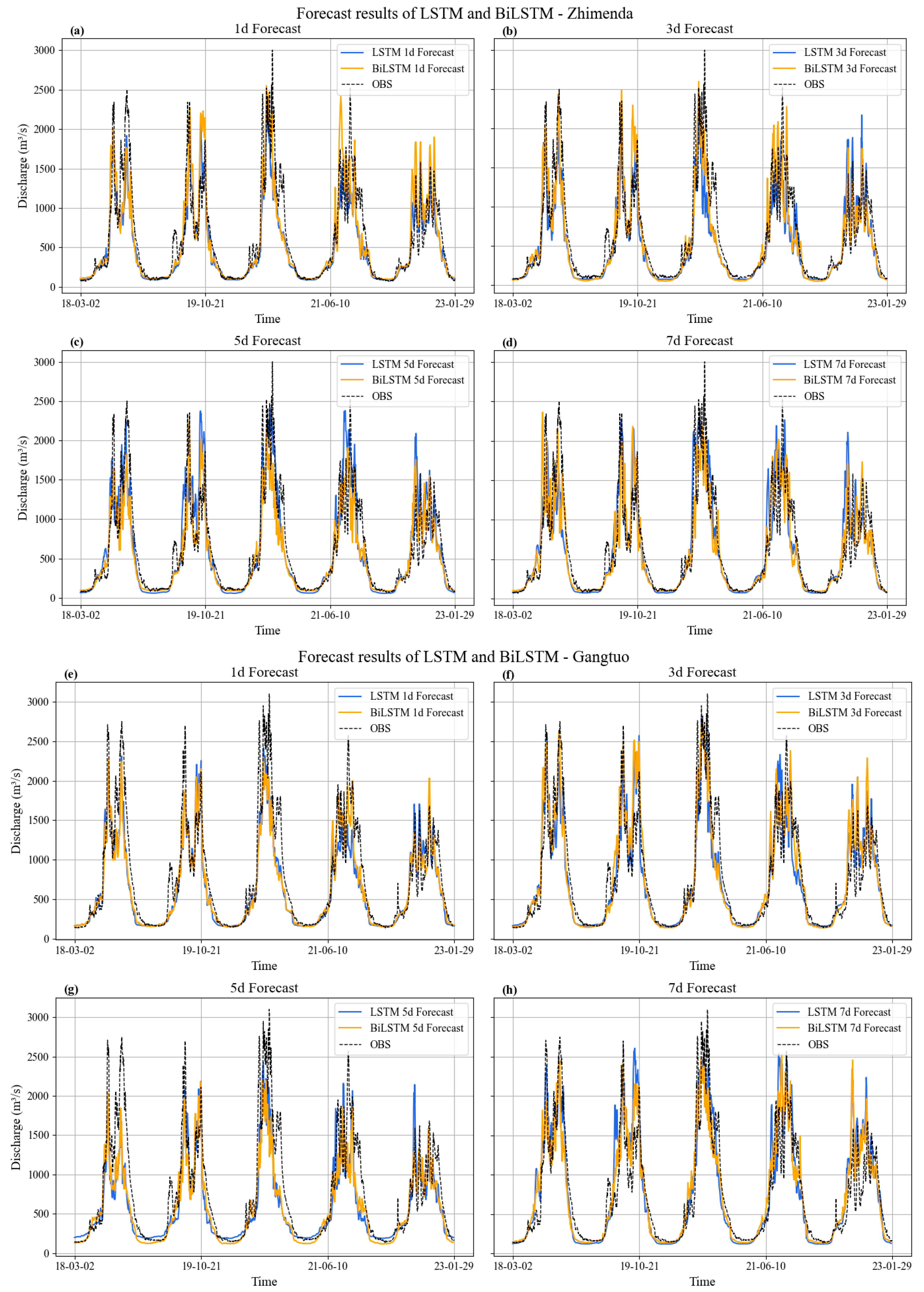
Both the LSTM and BiLSTM models effectively captured the characteristic peak–trough dynamics and seasonal patterns in the daily runoff forecasts across the 1 d to 7 d forecast periods at Zhimenda and Gangtuo Stations (Figure 10).

At Zhimenda, when the forecast period was 5 d, based on Figure 10c, the LSTM predictions consistently exceeded those of the BiLSTM model. However, this pattern did not hold for other forecast periods, and the simulated base flow process results were significantly lower than the observed values. For the second flood peak in 2019, both the LSTM and BiLSTM model substantially overestimated the peak magnitude and exhibited an accelerated flood response. For the major flood peak in 2020, both models markedly underestimated the peak value. At the 3 d forecast period, shown in Figure 10b, the LSTM model exhibited a marked underestimation of the drawdown phase relative to the observed data; at the 5 d forecast period, the BiLSTM model demonstrated a more rapid decline in the drawdown phase. For the 2022 flood peak, model results varied considerably across the four forecast periods. At the 1 d forecast period, the BiLSTM model significantly overestimated the flood peak magnitude, whereas the LSTM model exhibited more pronounced overestimation at the 3 d, 5 d, and 7 d forecast periods.

At Gangtuo Station, the 5 d forecast results, presented in Figure 10g, exhibited significant underestimation, with pronounced underestimation observed for all peak values during the test period. The 1 d forecast results also showed some degree of underestimation, though less severe than the 5 d forecasts. Moreover, similar to Zhimenda Station, the LSTM model exhibited an underestimation of base flow in the 5 d forecast results. The process lines for the 3 d and 7 d forecasts showed good fit. The LSTM and BiLSTM models demonstrated advantages in simulating runoff processes in different years: the LSTM model provided a better fit for the 2018 flood event, while the BiLSTM model performed better in simulating the 2020 flood event. For the 2019 flood process, the 1 d and 5 d forecasts did not exhibit the significant overestimation seen at the Zhimen Station, but both showed delayed flood response across the entire forecast period. Both LSTM and BiLSTM slightly underestimated the drawdown process compared to the observed flow rates.

At Zhimenda Station, the LSTM and BiLSTM models exhibited a marked contrast: systematically overestimating the 2019 secondary flood peak while underestimating the 2020 main flood peak. This reflects differing generalization capabilities across flood magnitudes. At Gangtuo Station, while the models did not exhibit the pronounced overestimation seen at Zhimenda Station, they generally underestimated flood crests and predicted faster drawdown rates. This indicates that differences in land surface conditions and basin confluence characteristics exerted a modulating effect on model performance.

The LSTM and BiLSTM models demonstrated strong capability in capturing the temporal evolution of runoff at individual stations. However, their independent data-driven frameworks, devoid of watershed-scale physical mechanisms, resulted in hydrologically inconsistent forecasts across the basin. This lack of spatial coherence is a direct consequence of their inability to learn interstation dependencies. Moreover, the pervasive baseflow underestimation by both models highlights a common structural weakness in simulating low-flow regimes and subsurface storage dynamics.

5. Discussion

5.1. Analysis of Model Performance Characteristics and Influencing Factors

In the alpine region of the Upper Jinsha River Basin, runoff processes exhibit strong seasonality and substantial intra-annual variability, shaped by complex topography, cryospheric dynamics, and seasonal precipitation. Under a unified evaluation framework, the BTOP, LSTM, and BiLSTM models demonstrate distinct performance characteristics, influenced collectively by watershed attributes, data quality, and model structure. The BTOP model, with its physics-based structure describing runoff generation and convergence, maintains robust water balance and long-term simulation stability in data-sparse, highly seasonal regions. However, it shows high sensitivity to input data quality and parameterization. When driven by insufficiently representative inputs, its simulations tend to reflect data artifacts rather than true basin processes, often resulting in systematic underestimation or lagged peak flows. In contrast, the LSTM and BiLSTM models capture temporal dependencies and nonlinear responses through end-to-end learning, achieving a higher overall accuracy than BTOP in daily-scale runoff simulation, particularly in capturing and reproducing flood peaks. In summary, BTOP is more suitable for long-term runoff simulation under data-constrained scenarios, whereas LSTM/BiLSTM show clear advantages in simulating extreme events and short-term dynamics. The complementary strengths of these approaches suggest that integrating physical constraints with data-driven methodologies may offer an effective pathway to improve simulation accuracy in complex catchments [24]. The findings of this study align with those reported by Kratzert et al. [47] and Xiang et al. [23], further validating the performance and limitations of the relevant models in runoff simulation and forecasting.

5.2. The Mechanism of BiLSTM in Flood Short-Term Forecasting

The BiLSTM model exhibited divergent performance during the training and test periods: it showed a slight advantage in the training period, but this advantage was not sustained during testing. The key structural strength of the model lies in its ability to process sequential data bidirectionally, enabling it to leverage both past and future contextual information during the training period. Theoretically, this architecture enhances the identification of complex temporal patterns such as wet–dry transitions, peak flows, and recession limbs, which explains its marginally superior performance in the training period. However, this study observed that the BiLSTM’s advantage diminished during the test period, with a more pronounced decline in NSE values compared to the unidirectional LSTM, indicating a potential tendency toward overfitting. This phenomenon can be attributed to the nature of the bidirectional mechanism: while the incorporation of future information during training period improves temporal feature extraction, such information is inherently unavailable in actual forecasting scenarios. As a result, the model’s generalization capability may be compromised, leading to reduced extrapolation accuracy and physical consistency in independent tests. Nevertheless, the degree of overfitting remains relatively limited, and the BiLSTM can still achieve results comparable to those of the LSTM in practical flood forecasting applications.

5.3. Simulation of Typical Flood Events and Performance Analysis of Multi-Timescale Forecasting

Representative flood events were selected for model comparison because the differences in model response—both in magnitude and timing—are most pronounced during peak flows and the surrounding hydrograph phases. The physically based BTOP model exhibited greater stability in reproducing peak magnitudes, a strength derived from its inherent water balance constraints. In contrast, the data-driven LSTM and BiLSTM models more accurately captured the timing of the peak and the shape of the hydrograph, but they consistently underestimated the peak magnitude itself. This performance divergence originates from the models’ fundamental structures. The deep learning models learn temporal mappings from data, which often results in smoother hydrographs that struggle to replicate abrupt, high-magnitude peaks. The physical model, by explicitly simulating runoff generation and flow routing, inherently conserves mass and is therefore better equipped to simulate peak discharges. This mechanistic difference is the root cause of their contrasting performances in flood event simulation.

5.4. Limitations and Future Research Directions

This study has several limitations. First, the simulation accuracy was likely constrained by the sparse network of meteorological stations, suggesting a need for future studies to incorporate high-resolution gridded datasets or satellite-based products. Second, the hyperparameters for the deep learning models were not extensively optimized for this specific basin, indicating that a systematic tuning campaign could improve performance. Finally, the limited physical interpretability of the data-driven models remains a challenge. Future work will focus on leveraging multi-source data fusion techniques and integrating in situ observations with satellite precipitation, evapotranspiration products, and atmospheric reanalysis data to build a more robust data foundation that mitigates the impact of spatial data gaps. Furthermore, we will develop tightly coupled hybrid models that systematically embed hydrological models within deep learning frameworks and conduct model interpretability analyses.

6. Conclusions

This study presents a comparative evaluation of the distributed physical model BTOP and the deep learning models LSTM/BiLSTM, using the Zhimenda and Gangtuo Stations in the Upper Jinsha River as a case study. The performance of both model types was assessed for runoff simulation, and the capability of deep learning models for short-term (1–7 d) forecasting was investigated. The main conclusions are as follows:

In daily-scale runoff simulation, the BTOP model demonstrated limitations in performance, constrained by input data quality and simplified representations of complex cryospheric processes. During the validation period, the NSE values for Zhimenda and Gangtuo stations were 0.57 and 0.62, respectively (calibration: 0.67 and 0.69). In contrast, the LSTM and BiLSTM models, with their superior ability to capture temporal dependencies and nonlinear relationships, achieved a higher overall accuracy in reproducing runoff processes. During the test period, they maintained high precision, with NSE values of 0.82 and 0.81 at Zhimenda Station, and 0.87 and 0.86 at Gangtuo Station.

For short-term forecasting, the LSTM and BiLSTM models showed comparable performance, with both effectively capturing temporal runoff patterns while exhibiting similar limitations in peak flow estimation and hydrological consistency. Although BiLSTM’s bidirectional architecture offers theoretical advantages during the training period, this capability becomes functionally constrained in real forecasting scenarios where future inputs are unavailable. Consequently, BiLSTM demonstrated no practical superiority over the simpler unidirectional LSTM in this application, with its slightly more pronounced performance decline from the training period to the test period suggesting a minor overfitting tendency without substantially affecting overall forecast quality.

During flood events, the models exhibited a distinct performance trade-off: the physics-based BTOP model demonstrated superior stability in reproducing peak magnitudes, while the data-driven models (LSTM and BiLSTM) more accurately captured the timing of peaks and the shape of the hydrograph. This fundamental divergence stems from their core structures—BTOP inherently conserves mass through physical equations, whereas the deep learning models learn smoothed temporal mappings that struggle to fully replicate abrupt, high-magnitude peaks.

In conclusion, this study confirms that deep learning models achieve superior accuracy in runoff simulation and flood characteristic capture compared to the physics-based BTOP model, solidifying their value for alpine hydrology. Furthermore, it reveals a fundamental complementarity between physical and deep learning models in runoff simulation and forecasting within complex alpine basins. Physics-based models like BTOP offer greater stability and interpretability in flood peak magnitude control and long-term sequence simulation, making them suitable for process mechanism analysis and long-term trend prediction. In contrast, data-driven models such as LSTM and BiLSTM excel in process morphology fitting and peak timing identification, proving particularly effective for runoff simulation and short-term forecasting in complex environments. Therefore, future efforts focus on hybrid approaches that merge their strengths. This work provides a systematic evidence base for such advancements, paving the way for more reliable hydrological forecasting in complex, data-scarce regions.