Estimating River Discharge from Remotely Sensed River Widths in Arid Regions of the Northern Slope of Kunlun Mountain

Abstract

Arid-region water resource management is hindered by severely inadequate river discharge monitoring, with effective observations of hydrological processes particularly lacking in narrow river channels. To overcome this bottleneck, this study proposes an integrated multi-model remote sensing retrieval framework and systematically evaluates the applicability of Manning’s equation, the At-Many-Stations Hydraulic Geometry (AHG) model, and the AHG’s relaxed form (AMHG) in typical arid-region rivers on the northern slope of the Kunlun Mountains. Runoff was estimated by integrating multi-source remote sensing imagery (Sentinel-2, Landsat-8, and Gaofen-1) on the Google Earth Engine platform and combining it with genetic algorithms for parameter optimization. The results indicate that Manning’s equation performed the best overall (RMSE = 21.78 m³/s, NSE = 0.94) and was highly robust to river width extraction errors, with Manning’s roughness coefficient having a significantly greater impact than the hydraulic slope. The AHG model can construct long-term discharge series based on limited measured data but is sensitive to the accuracy of river width extraction. Although the AMHG model improved the retrieval performance, its effectiveness was constrained by systematic biases in proxy variables. The study also found that the AHG exponent b in the rivers of this region exhibits high stability (coefficient of variation < 0.09), providing a theoretical basis for constructing a sustainable discharge monitoring system. The integrated method developed in this study offers a reliable technical pathway for dynamic hydrological monitoring and quantitative water resource management in data-scarce arid regions.

1. Introduction

Runoff is the primary form of available freshwater resources [1]. Hydrological stations serve as the main method for monitoring runoff, yet global coverage of these stations is limited [2,3]. Moreover, since 1980, the density of global hydrological stations has shown a declining trend, indicating a deterioration in monitoring capacity [4]. This problem is more pronounced in developing countries, especially in arid regions and high-altitude mountainous areas with low population density, where conditions are even worse [5,6]. Even in the United States, the number of hydrological stations has decreased by 25% [7]. Additionally, inefficient international data-sharing mechanisms hinder the utilization of existing observational data [8]. Therefore, there is an urgent need to develop alternative monitoring methods to compensate for the shortcomings of traditional hydrological station observations.

Remote sensing data, characterized by real-time capability, macroscopic perspective, periodicity, and low cost, offer a promising solution for runoff monitoring [9,10,11]. Remote sensing-based methods for runoff monitoring can be broadly categorized into several types: empirical stage–discharge relationships built using satellite altimetry data; empirical area–discharge relationships based on river inundation area; direct calculation methods using key parameters of hydraulic equations derived from remote sensing, such as the Manning equation; and the At-Many-Stations Hydraulic Geometry (AMHG) method proposed by Gleason and Smith. Consequently, remote sensing has been widely applied in river discharge estimation and has reached methodological maturity [12,13,14]. For instance, Gleason and Smith [15] successfully estimated discharge for 34 rivers globally using only remote sensing imagery. Hagemann et al. [16] validated the feasibility of AMHG–Manning for discharge estimation using remotely sensed river widths for 19 rivers. However, most successful applications have focused on large rivers [17,18,19], while research on discharge retrieval for narrow inland rivers in arid regions remains limited [20].

The northern slope of the Kunlun Mountains is a vital water source for the Tarim River Basin and a key ecological frontline along the Hexi Corridor–Taklimakan Desert margin. Its river runoff is primarily recharged by precipitation and snow/ice meltwater [21,22,23]. The general pattern shows spring droughts, summer floods, and severe seasonal water scarcity [24]. Recent studies have revealed significant alterations in regional hydrological processes and increasing variability in water resource availability. This poses substantial challenges for water resource management, which are further exacerbated by the limited capacity of the existing hydrological gauging network [25,26]. Therefore, there is a critical need for remote sensing-based methods to enhance the understanding of water resources and promote the coordinated development of water, ecology [27,28], and the economy. But, a key knowledge gap exists regarding the performance comparison and applicability of different retrieval models for narrow rivers in arid environments.

Previous studies have rarely conducted systematic evaluations of methods such as AHG, AMHG, and the Manning formula within a consistent multi-sensor observation framework in such environments. In this study, we aim to address this gap by focusing on inland rivers (with an average width of about 30 m) on the study area. We integrate multi-source remote sensing data and perform automated processing on the Google Earth Engine (GEE) platform. Through a comparative analysis of three models, we aim to (1) identify the most effective runoff retrieval method for arid regions; (2) reconstruct historical hydrological sequences; (3) establish a low-cost monitoring framework to support water resource management decisions in data-scarce basins. Therefore, this study seeks to promote the application of remote sensing-based runoff retrieval frameworks in narrow rivers of data-scarce arid areas through systematic comparative evaluation, providing a reliable and low-cost solution for hydrological monitoring in such regions.

2. Study Area, Data, and Methods

2.1. Study Area

As shown in Figure 1, the northern slope of the Kunlun Mountains, situated along the southern margin of Xinjiang’s Tarim Basin, serves as the primary water source for the Tarim River Basin and represents a transitional zone between Central Asia’s arid and alpine regions. The area is dominated by small and medium-sized rivers, with 76 rivers flowing into the Tarim Basin [29], but only 20 conventional hydrological stations monitor 9 major rivers. The study area includes three rivers with annual runoff exceeding 1 × 10⁹ m³—the Karakash, Yurungkash, and Qarqan Rivers—which collectively account for 50% of the regional discharge and serve as critical water sources for the oasis ecosystems along the southern Tarim Desert margin [23,29]. Selected virtual hydrological stations were positioned near river outlets relatively close to gauging stations to minimize channel loss effects. Site selection balanced mass conservation requirements for discharge calculations with observational needs for dynamic width variations, ultimately identifying representative reaches with significant width changes between wet and dry seasons and relatively straight channel morphology. These reaches exhibit typical mountainous river characteristics: exposed bedrock, sparse vegetation, and gravel-dominated V- or U-shaped incised channels with stable longitudinal slopes, minimal depth variation, and negligible sediment accumulation [30]. The stable geomorphic conditions and consistent hydraulic geometry ensure reliable discharge estimation across seasonal flow variations.

2.2. Date and Preprocessing

Based on the Copernicus Data Ecosystem platform (https://dataspace.copernicus.eu, accessed on 13 December 2024) and the Google Earth Engine COPERNICUS/S2_SR dataset, we retrieved and processed 737 cloud-free Sentinel-2 images of the study area from 2016 to 2024. The spatial resolution of Band 11 was enhanced from 20 m to 10 m using super-resolution reconstruction technology (SupReME), effectively improving the monitoring capability for medium-sized and small rivers [31].

Additionally, we acquired cloud-free Landsat-8 OLI data for the entire year of 2014 from the USGS platform (https://earthexplorer.usgs.gov, accessed on 13 March 2025). The panchromatic and multispectral images underwent radiometric calibration and geometric registration to eliminate sensor discrepancies and geometric distortions. The spatial resolution of the multispectral bands was uniformly enhanced to 15 m using Gram–Schmidt fusion algorithms, optimizing the spatial resolution of target bands while preserving spectral characteristics to improve land-cover identification [32,33].

Due to limited Sentinel-2 data availability in 2017 and significant cloud cover, the number of high-quality, cloud-free images for that year was insufficient. To ensure temporal continuity, we supplemented the dataset with GF1-WFV multispectral images (original resolution: 16 m) from the China Centre for Resources Satellite Data and Application (https://data.cresda.cn/#/home, accessed on 21 March 2025) for 2015 and 2017. Remote sensing imagery details are shown in

Table 1. Remote sensing imagery details.

Date Source	Selected Band	Spatial Resolution	Enhanced Resolution	Fusion Method	Temporal Resolution	Selected Time Period
Sentinel-2	Visible (B2 B3 B4) NIR (B8) SWIR (B11)	10/20 m	10 m	RS (Super- Resolution)	5/10 d	2016–2024
Landat-8	Visible (B2 B3 B4) NIR (B5) SWIR (B6 B7) PAN (B8)	15/30 m	15 m	GS (Gram- Schmidt)	16 d	2014
GF1	Visible (B1 B2 B3) NIR (B4)	16 m			4 d	2015/2017

Note: Visible denotes the visible spectral bands; NIR refers to the near-infrared region; SWIR indicates the shortwave infrared wavelengths. For Sentinel-2 and Landsat-8, bands B2 (Blue), B3 (Green), and B4 (Red) represent the visible spectrum. Similarly, in GF-1, bands B1 (Blue), B2 (Green), and B3 (Red) correspond to the visible spectrum.

.

Topographic data were derived from the Copernicus Digital Elevation Model (Copernicus DEM, 30 m resolution, vertical accuracy < 4 m) provided by the European Union’s Copernicus Programme (https://dataspace.copernicus.eu/explore-data/data-collections/copernicus-contributing-missions/collections-description/COP-DEM, accessed on 8 December 2024). This dataset enables the extraction of cross-sectional river profiles at any location within the watershed and is widely used in basin terrain modeling [34]. Streamflow and water level observations were obtained from hydrological stations, all located near the study river channels to minimize channel loss.

2.3. Methods

2.3.1. River Width Extraction

GEE is a powerful cloud-based geospatial analysis platform that integrates vast amounts of remote sensing data and supports efficient processing of long-term time-series imagery (accessed on 23 March 2024). Its automated computation and analysis capabilities significantly enhance the efficiency of remote sensing data processing [35].

River width is a critical parameter for runoff retrieval. In this study, we implemented an automated river width extraction method based on the cloud-based geospatial analysis platform GEE. By querying the GEE data catalog, we obtained 737 cloud-free Sentinel-2 images of the three target rivers from 2018 to 2024. To compensate for data gaps, 416 additional images from Landsat-8 and GF-1 (Gaofen-1) satellites were incorporated, with all images excluding ice-covered periods. For water body extraction, a multi-band thresholding method was applied, utilizing either the Revised Normalized Difference Water Index (RNDWI) or the traditional Normalized Difference Water Index (NDWI), depending on data source characteristics: When shortwave infrared (SWIR) bands were available, RNDWI was prioritized to reduce mixed-pixel effects and topographic shadow interference, thereby improving water-land boundary extraction accuracy. When SWIR bands were unavailable, NDWI was used to suppress vegetation reflectance signals, though this method remains susceptible to topographic shadows and other interferences [36].

An adaptive threshold segmentation approach based on Otsu’s algorithm was applied to the water index imagery. By maximizing inter-class variance and minimizing intra-class variance, the optimal segmentation threshold was automatically determined, enabling binary classification of water and non-water areas. Compared to fixed-threshold methods, Otsu’s algorithm better adapts to spectral variations across different regions and time-series images, enhancing the robustness and accuracy of water body extraction Finally, river width was calculated using the water area method, as shown in Equation (1):

$$A_w={\displaystyle \frac{P_w{A}_t}{p_t}}$$

(1)

where $A_w$ represents the water area (m²), $P_w$ denotes the number of water pixels, $A_t$ is the total study area (m²), $p_t$ refers to the total number of pixels in the study area. The river width ($w_R$) can thus be derived as:

$$w_R={\displaystyle \frac{A_w}{L}}$$

(2)

where $w_R$ is the river width, L is the length of the specified river reach. Given that most rivers in the study area are relatively narrow (typically less than 3 pixels wide during dry seasons), the mixed-pixel effect significantly impacts the accuracy of traditional remote sensing methods. To address this, we employed the Water Area Method for river width extract, which effectively reduces systematic errors caused by mixed pixels [35]. For river segments with significant extraction errors (approximately 15% of the total samples) due to cloud cover, shadows, or vegetation interference, manual visual interpretation combined with GIS digitization was applied to ensure data reliability. All manual interpretations followed standardized criteria and were independently conducted by two professionals, with cross-validation achieving over 90% consistency.

2.3.2. At a Station Hydraulic Geometry (AHG)

Although remote sensing imagery cannot directly measure discharge, it enables efficient extraction of river width parameters at any cross-section. Based on the AHG theory proposed by Leopold and Maddock, there exists a significant exponential relationship between characteristic river width and discharge [37]. This relationship can be expressed by Equation (3), where $\mathrm{a}$ and $\mathrm{b}$ are empirical parameters unique to each cross-section, derived from long-term river width observations and corresponding ground-measured discharge data.

The AHG theory has been widely validated in natural river systems [38], providing a scientific foundation for using remotely sensed river width data to achieve long-term discharge monitoring. Compared to traditional hydrological monitoring methods, the AHG relationship model overcomes spatial limitations by enabling non-contact discharge estimation at any river section, offering a novel technical approach to watershed hydrological monitoring [39].

$$w=a{Q}^b$$

(3)

$$Q={\left({\displaystyle \frac{w}{a}}\right)}^{{\displaystyle \frac{1}{b}}}$$

(4)

The AHG parameters at different locations along the same river are not spatially independent but exhibit log-linear correlations, where parameter $\mathrm{b}$ can be expressed as a function of parameter a. When the AHG fitting curves of cross-sections intersect at a common point in hydraulic space, an At-Many-Stations Hydraulic Geometry (AMHG) relationship is established [40]. This phenomenon has been demonstrated to be prevalent across various river types [15]. The discovery of AMHG represents a significant breakthrough for remote sensing-based discharge estimation, as it can effectively reduce required hydraulic geometry parameters and decrease model complexity [41]. By leveraging repeated observations from remote sensing satellites, river discharge can be reliably estimated without depending on traditional ground-based hydrological measurements [42]. This approach enables continuous, large-scale discharge monitoring while overcoming the spatial limitations of conventional gauge stations, making it particularly valuable for ungauged or data-scarce basins. The AMHG relationship as described by Equation (5):

$$F=a_{x1,x2\dots \dots xn}{E}^{bx1x2\dots x_n}$$

(5)

where $x1,x2\dots \dots xn$ represent the spatial index positions along the river cross-sections, $\mathrm{a}$ and $\mathrm{b}$ are the empirical AHG parameters, and $F$ and $E$ are river-specific constants defining the intercept and slope of the AMHG relationship. The constant $F$ can be approximated using river width measurements along the cross-sections. By substituting $F$ with its width-based approximation and taking the logarithm of both sides, Equation (5) can be reformulated into the Width AMHG:

$${ b}_x=-{\displaystyle \frac{1}{\mathit{log}\left(E\right)}}\times \mathit{log}\left(a_x\right)+{\displaystyle \frac{1}{\mathit{log}\left(E\right)}}\times \mathit{log}\left(W_{mean}\right)$$

(6)

$$Slope=-{\displaystyle \frac{1}{\mathit{log}\left(E\right)}}$$

(7)

$$Intercept={\displaystyle \frac{1}{\mathit{log}\left(E\right)}}\times \mathit{log}\left(W_{mean}\right)$$

(8)

$$b_x=Slope\times \mathit{log}\left(a_x\right)+Intercept$$

(9)

where for each river or reach, $E$ is a fixed and unique constant, with its units varying across cross-sections according to the exponent $b$, reflecting the unified scaling law of AHG parameters. $W_{mean}$ (m) represents the mean river width across all cross-sections. While $E$ is typically difficult to measure directly, Gleason and Smith [15] proposed a robust empirical proxy, $y$, which successfully predicts the true AMHG slope. The proxy $y$ (where $y$ = $\mathit{log}\left(E\right)$) does not require prior knowledge or ground-based data. Instead, it can be derived solely from repeated remote sensing observations of river widths. The parameters $P$ and $y$ are calibrated via Equation (10) by fitting the maximum and minimum width variations across all cross-sections.

$$\max \left({\mathrm{w}}_{\mathrm{x}1,\mathrm{x}2\dots \mathrm{x}\mathrm{n}}\right)=\mathrm{P}{\left(\max {\left({\mathrm{w}}_{\mathrm{x}1,\mathrm{x}2\dots \mathrm{x}\mathrm{n}}\right)}^2-\min {\left({\mathrm{w}}_{\mathrm{x}1,\mathrm{x}2\dots \mathrm{x}\mathrm{n}}\right)}^2\right)}^{\mathrm{y}}$$

(10)

The AMHG approach overcomes the limitations of single-station AHG by capturing the integrated hydraulic characteristics of entire river reaches without relying on historical ground-based observations. When implementing AMHG for discharge estimation, the number of cross-sections and their spatial distribution intervals have a relatively minor influence on model performance when compared to data quality and cross-section representativeness, which are critical factors. The selected study reaches had lengths between 5 and 11 km to ensure that the chosen cross-sections adequately represented downstream hydraulic geometry variations while excluding anthropogenically modified segments. Previous studies [15,43] demonstrated that even a small number of strategically positioned cross-sections can produce reliable AMHG relationships, which informed our methodology of selecting 11 representative cross-sections per river.

2.3.3. Genetic Algorithm Technique for River Discharge Estimation

The genetic algorithm was employed to optimize the coefficient $\mathrm{a}$ and exponent $\mathrm{b}$ for each pair of cross-sections, with initial solutions generated through the AMHG relationship. Solutions failing to meet the discharge range criteria were discarded. After initializing a population of 10 chromosomes, fitness evaluation (minimizing discharge differences) was conducted to screen chromosomes. Through crossover, mutation, and iterative optimization (50 generations), four optimal parameters were obtained. To enhance reliability, each cross-section pair underwent 50 independent GA optimizations, yielding 100 sets of parameter estimates. Subsequently, the optimization process was extended to all cross-section combinations within the river reach, generating $\left({\mathrm{n}}^2-\mathrm{n}\right)$ × (num GA) AHG parameter estimates and $\left({\mathrm{n}}^2-\mathrm{n}\right)$× (num GA) direct discharge estimates, thereby minimizing discharge differences across different cross-sections. The parameter settings of the genetic algorithm refer to the study by Rao et al. [42], with specific parameters shown in

Table 2. Genetic Algorithm Parameter.

Parameter Category	Parameter Name	Value
Genetic Algorithm	Population Size	20
	Maximum Generations	60
	Crossover Rate	0.8
	Mutation Rate	0.1
	Tournament Size	3
Boundary Constraints	$\mathrm{a}$ (coefficient)	[0.01, 100]
	$\mathrm{b}$ (coefficient)	[0.01, 1]
	$\mathrm{b}$ Validation Threshold	50%
	Initial Q Range	[10, 600] m3/s
	Q Validation Threshold	50%

Note: The solution space for the value of $\mathrm{b}$ is allowed to expand by 50% under the condition that it conforms to the AMHG relationship. This value is designed based on the relative difference between the actual AHG $\mathrm{b}$ value and the $\mathrm{b}$ value determined by the AMHG relationship.

.

$\mathrm{a}$$\mathrm{b}$$\mathrm{b}$ Since the parameter E in Equation (5) can be derived from the fitted exponent proxy $\mathrm{y}$ in Equation (9), AMHG can be readily obtained, thereby constraining the possible ranges of the parameters $\mathrm{a}$ and $\mathrm{b}$. However, the proxy y does not strictly equal the specific constant $\mathrm{E}$, particularly for arid-region rivers, where significant errors may occur [15,43]. Restricting the solutions for $\mathrm{a}$ and $\mathrm{b}$ strictly within the AMHG relationship derived from $\mathrm{y}$ might lead to discharge retrieval results that deviate from actual conditions. Therefore, parameter adjustments were permitted within a certain range. Optimal parameter solutions were generated under two scenarios: relaxed and strict AMHG constraints. In both cases, the median and mean values of the optimized $\mathrm{a}$ and $\mathrm{b}$ solutions were used to estimate discharge. Regardless of the method employed, the final discharge estimates represented average runoff values across n cross-sections.

2.3.4. Manning Equation for River Discharge Estimation

The Manning–Strickler formula serves as an empirical equation for calculating the average velocity or discharge in open-channel uniform flow [44], and it is widely used in discharge estimation [45], which is formulated as

$$v=C{R}^{2/3}{J}^{1/2}$$

(11)

The Manning–Strickler formula (Equation (11)) describes the mean cross-sectional flow velocity ($v$, m³/s), where $C$ represents the Chezy coefficient characterizing comprehensive flow resistance, $\mathrm{R}$ denotes the hydraulic radius (m), and $\mathrm{J}$ indicates the energy slope representing energy loss per unit channel length. The Chezy coefficient can be derived from Manning’s equation (Equation (12)), while the hydraulic radius and energy slope are calculated using Equations (13) and (14):

$$C={\displaystyle \frac{1}{n}}{R}^{1/6}$$

(12)

$$R={\displaystyle \frac{A}{P}}$$

(13)

$$J={\displaystyle \frac{\mathsf{\Delta }h}{L}}={\displaystyle \frac{h_{up}-h_{down}}{L}}$$

(14)

where $n$ represents Manning’s roughness coefficient (dimensionless), $A$ denotes the cross-sectional flow area (m²), and $P$ is the wetted perimeter (m), while $h_{up}$ and $h_{down}$ correspond to upstream and downstream water surface elevations, respectively, with $L$ being the reach length (m). The discharge calculation follows Equation (15):

$$Q=v\cdot A={\displaystyle \frac{1}{n}}A{R}^{2∕3}{J}^{{\displaystyle \frac{1}{2}}}$$

(15)

The cross-sectional area A is determined using the “section geometry approximation method,” which combines channel elevation information extracted from the DEM and estimated water level values. Based on the DEM data, the typical cross-sections of the study reach are generalized into regular geometric shapes such as trapezoidal or parabolic forms. With the known river width, the cross-sectional area is calculated according to the generalized geometry and the water level corresponding to the river width. The hydraulic slope was derived from Copernicus DEM data, with sufficiently long river reaches selected to minimize errors in relative elevation measurements. Based on Equation (14), the calculated hydraulic slopes were 5 m km⁻¹, 12 m km⁻¹, and 20 m km⁻¹ for the Karakash, Yulongkash, and Qarqan Rivers, respectively. Manning’s roughness coefficients ($n$) were estimated through remote sensing observations combined with standard reference values from Chow’s classification tables, yielding values of 0.052 for the Karakash River and 0.035 for both the Yulongkash and Qarqan Rivers.

2.3.5. Model Accuracy Evaluation

The performance of the discharge retrieval model was evaluated using four statistical metrics: (1) the Nash–Sutcliffe efficiency coefficient ($\mathrm{N}\mathrm{S}\mathrm{E}$), which quantifies the model’s predictive accuracy relative to observed data variance; (2) root mean square error ($\mathrm{R}\mathrm{M}\mathrm{S}\mathrm{E}$), measuring absolute prediction errors in discharge units (m³/s); (3) relative root mean square error ($\mathrm{R}\mathrm{R}\mathrm{M}\mathrm{S}\mathrm{E}$), expressing normalized error magnitude as a percentage of observed mean discharge; and (4) coefficient of determination (${\mathrm{R}}^2$), assessing the proportion of variance explained by the model. This multi-metric approach is formulated as

$$RMSE=\sqrt{{\displaystyle \frac{{\sum }_{i=1}^n{\left(y_i-{\widehat{y}}_i\right)}^2}{n}}}$$

(16)

$$RRMSE=\sqrt{{\displaystyle \frac{\frac{1}{n}{\sum }_{i=1}^n{\left(y_i-{\widehat{y}}_i\right)}^2}{\overline{y}}}}$$

(17)

$$NSE=1{\displaystyle -}{\displaystyle \frac{{\sum }_{i=1}^n{\left(y_i-y_i^{pred}\right)}^2}{{\sum }_{i=1}^n{\left(y_i-\overline{y}\right)}^2}}$$

(18)

$$R^2=1-{\displaystyle \frac{\sum _{i=1}^n{\left(y_i-{\widehat{y}}_i\right)}^2}{\sum _{i=1}^{\overline{n}}{\left(y_i-\overline{y}\right)}^2}}$$

(19)

In this study, $y_i$ represents the simulated value of discharge, ${\widehat{y}}_i$ denotes the ground-measured value, ${ y}_i^{pred}$ is the value predicted by the retrieval model, $\overline{y}$ is the mean observed discharge, and $n$ is the sample size. This standard notation ensures consistent representation of data and model outputs in hydrological analyses.

3. Results

3.1. AHG Characteristics and Discharge Estimation Results

3.1.1. Temporal Variation Characteristics of AHG

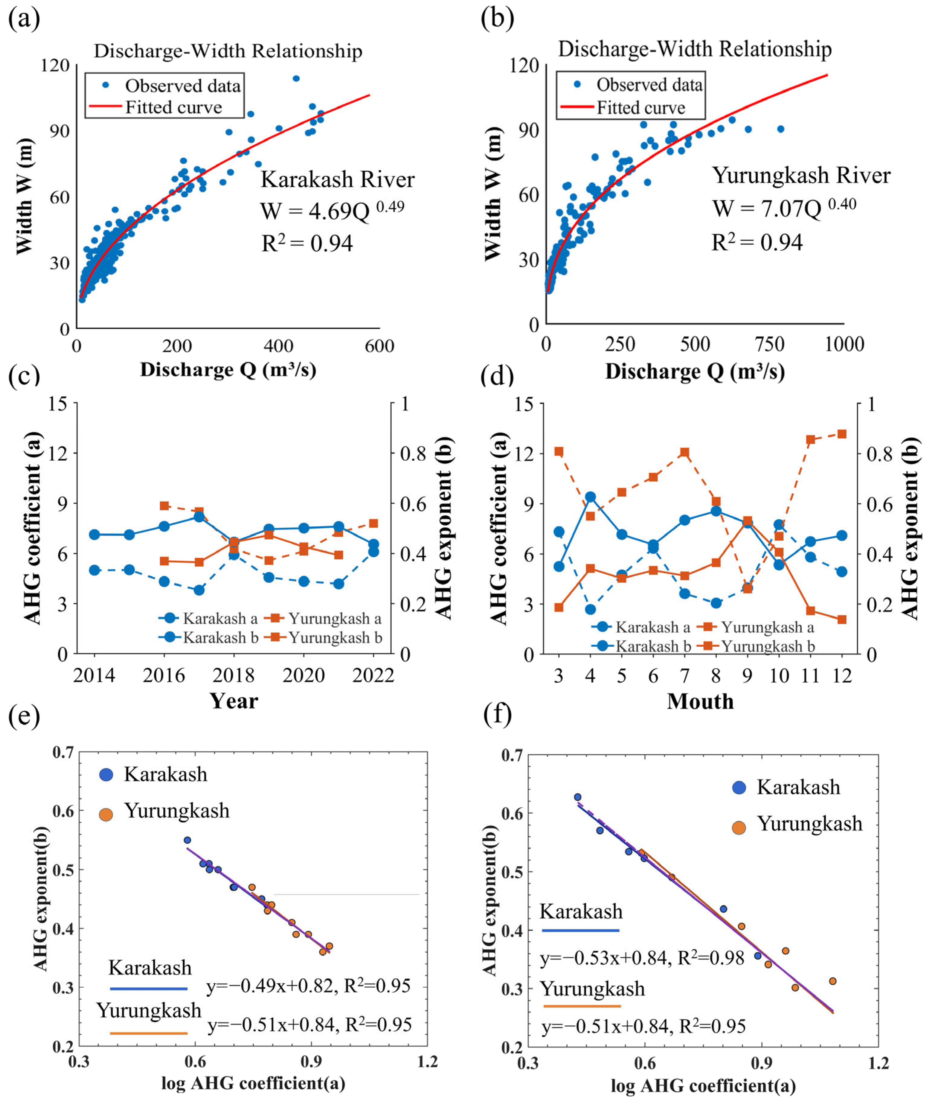
The discharge–width relationship for major rivers indicates significant spatial variations in channel morphology and hydraulic geometry parameters in the study area. Generally, arid regions exhibit relatively high AHG indices [39]. As shown in Figure 2a, the multi-year fitted AHG exponent $\mathrm{b}$ for the Karakash River is 0.49, with an interannual range of 0.44–0.55 in Figure 2c. However, the standard deviation of the AHG index is only 0.032, and the coefficient of variation (CV) is 6.53%. For the Yurungkash River, as shown in Figure 2b,c, the multi-year fitted AHG exponent $\mathrm{b}$ is 0.40, with an interannual range of 0.36–0.47, a standard deviation of 0.038, and a CV of 5.85%. Compared to the interannual variability of exponent $\mathrm{b}$ in humid regions [44], the AHG indices of these two arid-region rivers show very small interannual fluctuations, demonstrating high stability.

As shown in Figure 2e,f, a clear log-linear relationship exists between the AHG exponent $\mathrm{b}$ and coefficient $\mathrm{a}$, both within individual cross-sections and between different cross-sections over time. The ranges of the same AHG parameters are very similar, possibly because of the comparable drainage areas of the basins [46].

In contrast to interannual variations, the intra-annual fluctuations of the AHG exponent $\mathrm{b}$ are more pronounced, as shown in Figure 2d. The standard deviations for the Karakash and Yurungkash Rivers are 0.08 and 0.11, with CVs of 17.43% and 36.40%, respectively. During the wet season (June–September), the exponent $\mathrm{b}$ increases significantly, while it decreases during the dry season (December–February), exhibiting an overall convex pattern intra-annually. The goodness-of-fit for AHG relationships also varies seasonally, with better performance during the wet season (R² > 0.80) than during the dry season (R² < 0.45). An anomalously low fit (R² < 0.40) was observed for the Yurungkash River in June, but after excluding the outlier from June 2018, the R² improved to 0.82.

Overall, the AHG parameters of rivers exhibit distinct spatiotemporal heterogeneity. The annual variation coefficients of the AHG exponent b are below 7% for both the Karakash and Yurungkash Rivers, demonstrating high temporal stability in the stable channels of this arid region. This stability likely stems from the bedrock or cobble composition of the riverbeds in the study area, which provides strong erosion resistance and results in minimal interannual changes in channel morphology. Notably, although the goodness-of-fit for AHG decreases during the dry season (R² < 0.45), the parameters still maintain a certain log-linear co-variation pattern. This indicates that the AHG structure maintains hydraulic consistency across seasons in arid-region rivers, providing a structural basis for model adjustments during low-flow periods.

3.1.2. Estimation Results of the AHG Model

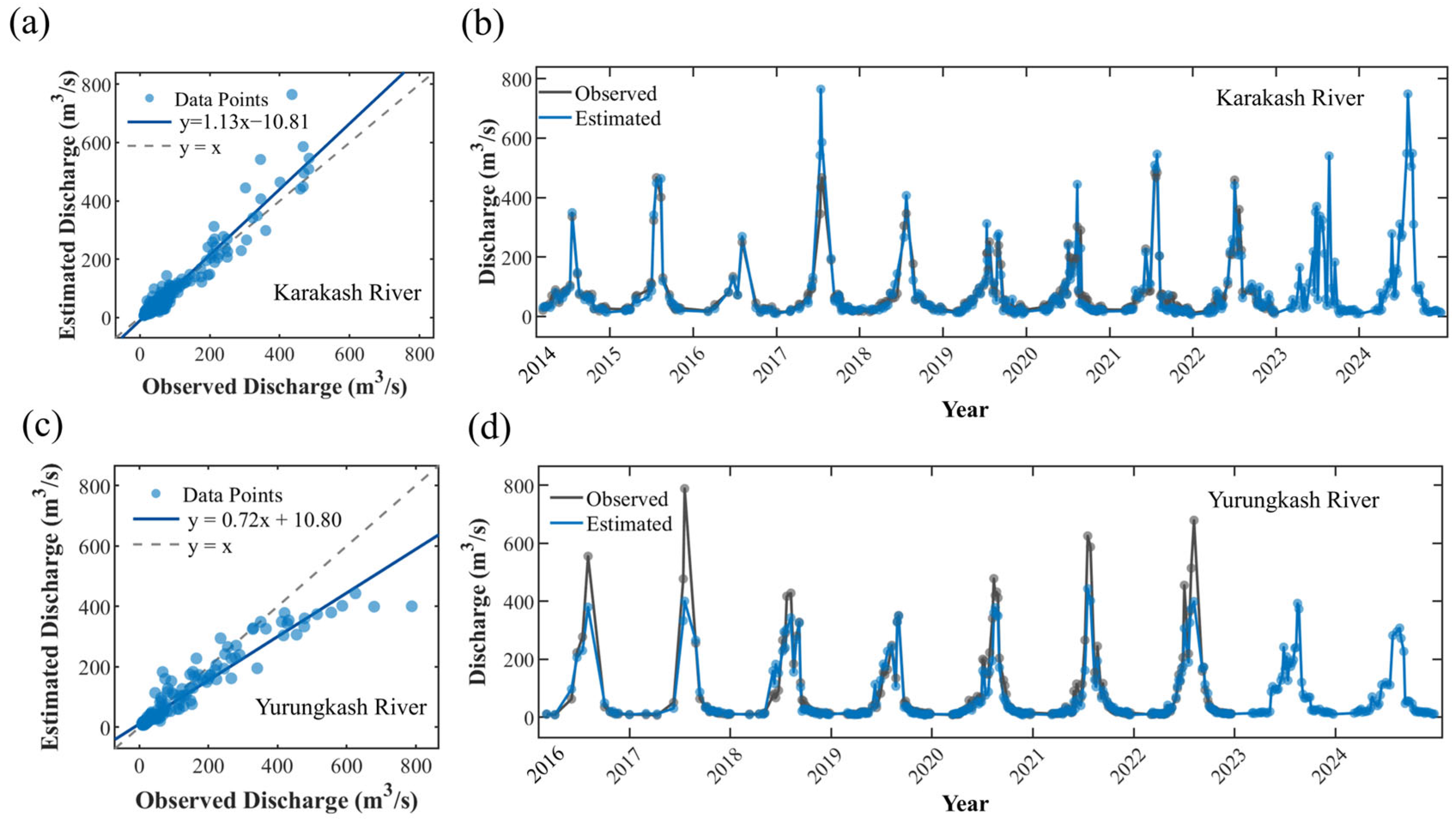
To discuss the AHG model’s ability to invert river discharge with limited data, hydrological station observation data from a single year were used to calibrate the AHG parameters, while data from other years served as the validation set. The validation results of the single-year AHG exponent model are listed in

Table 3. Performance Evaluation of Single-Year AHG Model Discharge Retrieval.

River	Indicators	2014	2015	2016	2017	2018	2019	2020	2021	2022
Yurungkash	Num image	-	-	12	20	35	43	48	43	45
	RMSE (m3/s)	-	-	35.10	47.38	48.02	55.63	39.26	43.57	35.70
	RRMSE (%)	-	-	41.69	56.27	57.03	66.07	46.63	51.75	42.40
	NSE	-	-	0.93	0.87	0.87	0.82	0.91	0.89	0.93
Karakash	Num Image	26	21	14	31	28	43	44	40	41
	RMSE (m3/s)	29.08	28.88	23.90	27.44	31.91	24.57	27.25	26.72	36.25
	RRMSE (%)	36.62	36.36	30.09	34.55	40.18	30.93	34.31	33.65	45.64
	NSE	0.90	0.90	0.93	0.91	0.88	0.93	0.91	0.92	0.85

and presented in Figure 3. For the Yurungkash River, the single-year AHG model has an average RMSE of 43.52 m³/s, an average RMMSE of 51.69%, and an average NSE of 0.89; for the Karakash River, the corresponding indicators are 28.44 m³/s, 35.82%, and 0.90, respectively, indicating excellent model fitting performance for the Karakash River. It is particularly noteworthy that although only 13 cloud-free remote sensing images were available as data in 2016, the NSE values of the single-year AHG exponent model for both rivers still reached 0.93. The effectiveness of the AHG model is not related to the quantity of collected effective river width data, but rather to whether there are sufficient images that can reflect river width changes in different periods. Therefore, when limited flow observation data are sufficient to cover both the dry and wet seasons of the river, and the acquisition dates of the images are close to the observation dates of the flow, effective long-term runoff retrieval is still possible [47].

3.2. Estimation Results of the Width AMHG Model

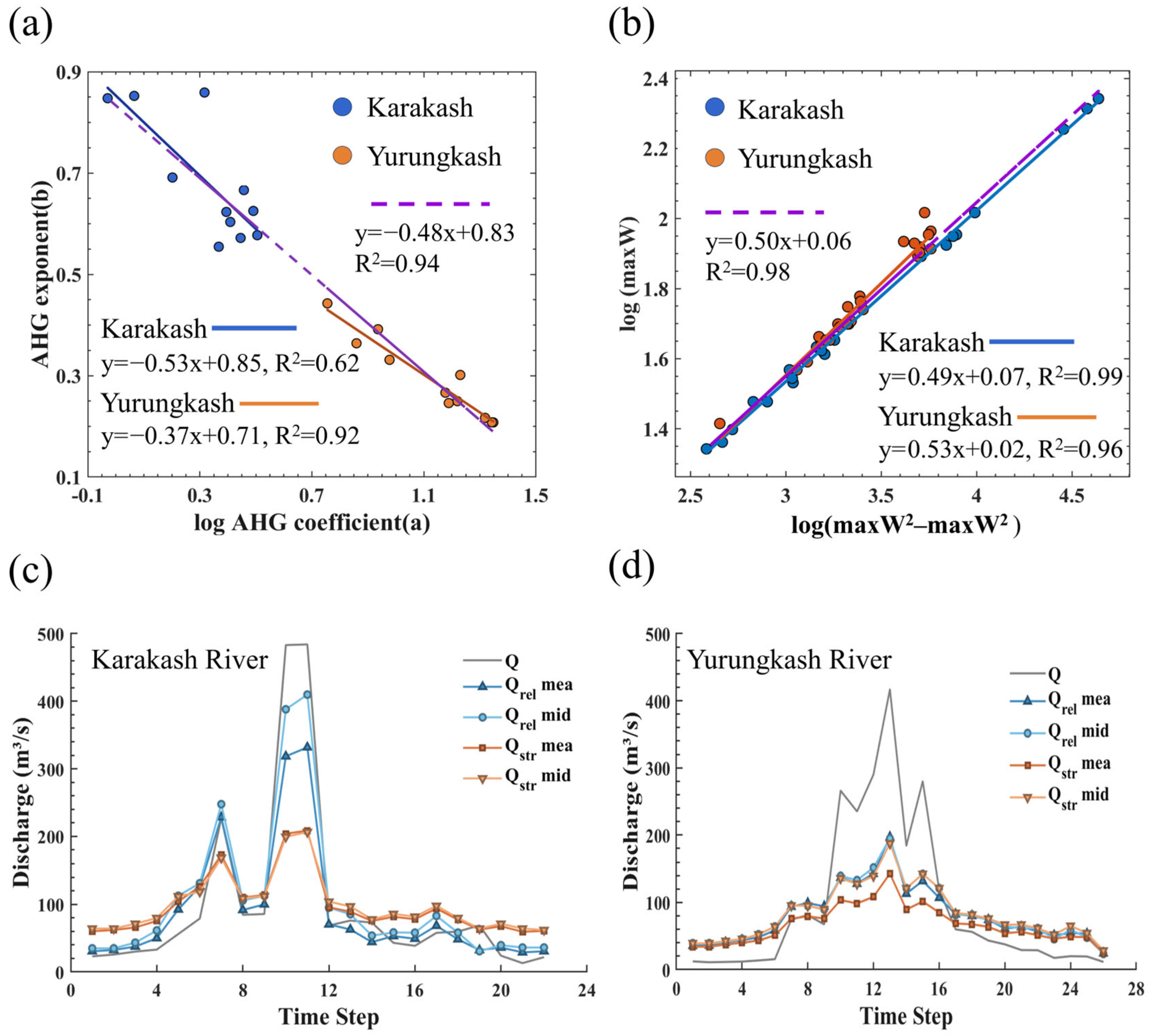
The AMHG relationships derived from 2019 data for the Karakash and Yurungkash Rivers are shown in Figure 4a. The rivers in the arid region exhibit clear AMHG relationships (correlation coefficient > 0.6), indicating that AMHG can predict AHG parameters with reasonable accuracy [48]. The Karakash River has a relatively low AMHG R² of 0.62, but its best discharge estimation yields an RRMSE (Relative Root Mean Square Error) of 35.78%. In contrast, the Yurungkash River has a much higher AMHG R² of 0.92, yet its best discharge estimation RRMSE reaches 77.50%. This suggests that the strength of the AMHG relationship has little impact on the discharge estimation accuracy, consistent with the findings of Barber and Gleason [49] and Gleason and Smith [15].

Using Equation (10), we established an RS Slope regression relationship, shown in Figure 4b. However, the proxy parameter $\mathrm{y}$ was not as robust in theory as expected. It performed well for the Karakash River, with the derived AMHG slope differing by only 0.03 from the actual value, but poorly for the Yurungkash River. When the proxy $\mathrm{y}$ was close to the theoretical empirical value $E$, the estimated discharge better reflected the observed discharge variations. The suboptimal performance of the AMHG method in these rivers may be attributed to factors such as arid climate conditions, intensified infiltration and evaporation, biases in the proxy parameter $y$, high variability in extreme flows, sensitivity to river width measurement errors, and the potential presence of non-mass-conserving hydrological processes [15,50]. Additionally, Peignoir et al. [51] suggested that the performance of AMHG exhibits a strong positive correlation with the geomorphic factor ($b$) of river channels and a negative correlation with climatic aridity, while it is weakly correlated with factors such as mean river width, seasonal variations in river width, and vegetation coverage. These findings appear to provide a plausible explanation for a seemingly contradictory phenomenon: although arid regions are generally considered areas where the AMHG retrieval model fails [15], the model still achieves relatively accurate discharge estimates for the Karakash River. This is because more-arid regions tend to exhibit higher $b$ values [39], which can compensate for the negative impacts of climatic aridity, thereby maintaining the predictive accuracy of the model.

We investigated the influence of the proxy variable $y$ on the AMHG method by comparing different constraint conditions. Specifically, we examined two scenarios:

1.

Strict AMHG constraints: $y$ = $E$ (theoretical expected value), with all $\mathrm{a}$ and $\mathrm{b}$ values strictly constrained by the AMHG relationship.

2.

Relaxed AMHG constraints: Allowing $\mathrm{y}$ to deviate from $E$ and expanding the optimization range of parameter $\mathrm{b}$ (solved via Equation (9)) by ±50%, enabling the AHG exponent solutions to approach the true optimal values even if deviating from $E$.

Table 4. Accuracy Assessment of the AMHG-GA Method.

River	Method	RMSE (m3/s)	RRMSE (%)	NSE
Karakashi	Qrel mean	52.50	53.58	0.83
	Qrel mid	35.05	35.78	0.93
	Qstr mean	90.34	92.21	0.51
	Qstr mid	92.38	94.29	0.49
Yurungkash	Qrel mean	73.64	79.36	0.56
	Qrel mid	71.91	77.50	0.58
	Qstr mean	103.17	111.19	0.13
	Qstr mid	98.15	105.77	0.21

shows that AMHG constraints significantly affect estimation accuracy. Under strict AMHG constraints, both the Karakash and Yurungkash Rivers exhibited RRMSE values exceeding 90%, indicating substantial estimation bias under these conditions. However, when AMHG constraints were relaxed, estimation performance improved notably—especially when the proxy $y$ was close to the true $E$ value. For example, in the Karakash River basin, the Qrel-mid RRMSE under relaxed AMHG constraints decreased sharply from 92.38% to 35.78%.

Comparing the performance of the four discharge estimation methods, the Qrel-mid method demonstrated the highest accuracy. Nevertheless, it failed to correctly capture peak flows, consistently underestimating them.

3.3. Estimation Results of the Manning-Strickle Equation

The runoff reconstruction model based on Manning’s formula demonstrated strong overall performance, with NSE values all exceeding 0.93. Its superiority primarily lies in the direct representation of open-channel hydrodynamic physical processes. The study area features exposed bedrock and a riverbed composed mainly of gravel. These relatively stable and erosion-resistant boundary conditions enable parameters such as Manning’s roughness coefficient (n) and hydraulic slope (S) to maintain good stability over interannual scales. Consequently, Manning’s formula can more realistically simulate the synergistic changes between flow velocity and cross-sectional area as discharge increases, thereby successfully capturing flood-peak information during high-flow periods [52]. Its strong robustness to river width errors further demonstrates the advantages of physics-based models in addressing uncertainties associated with remote sensing input data.

Specifically, the simulation accuracy for the Karakash River was superior to that for the Yulong Kash River, with the former having lower RMSE (21.78 m³/s) and RRMSE (27.43%) compared to the latter (RMSE = 28.15 m³/s, RRMSE = 32.18%). Simulation performance was excellent for both rivers during high-flow periods (July to September). However, systematic biases occurred in low-flow months (October to February), with negative NSE values and an almost complete failure to capture low-flow information. Model reliability declined sharply when the mean river width was <30 m.

The Yulong Kash River showed an abnormally high RRMSE of 56.62% in June, with an NSE of only −0.19, primarily influenced by an outlier in 2018. After removing this outlier, the overall RRMSE for June decreased to 24.74%, and NSE increased to 0.75, indicating a significant impact of outliers on model performance. A comparison of remote sensing imagery from June 2018 revealed a notably expanded river width in the Yulong Kash River during that period, resembling the river morphology typical of historical high-flow seasons. Additionally, the measured discharge data showed a clear deviation from the historical trend for the same period. Therefore, the anomaly in June 2018 may be attributed to instrumental malfunction.

Since only monthly mean discharge data were available for the Qarqan River and remote sensing-derived discharge represents instantaneous measurements at the time of satellite overpass, direct comparison was inappropriate. Instead, multiple instantaneous remote sensing discharge estimates were analyzed for consistency with monthly mean gauge data trends to assess retrieval reliability. As shown in Figure 5e, remote sensing-derived discharge closely followed the variation trends of gauge-based monthly means. For further validation, the arithmetic mean of all available instantaneous remote sensing discharge values within each month was computed and quantitatively compared with the gauge-based monthly mean. The results yielded an RMSE of 7.51 m³/s, RRMSE of 26.31%, and NSE of 0.75, indicating that despite the inherent scale mismatch between instantaneous and monthly data, remote sensing retrievals effectively captured the hydrological dynamics of the Qarqan River. Given the inherent limitations of scale discrepancy, the result for the Qarqan River was obtained not to validate absolute accuracy but to provide a scientific reference for assessing the applicability of the Manning formula in the region.

3.4. Sensitivity Analysis

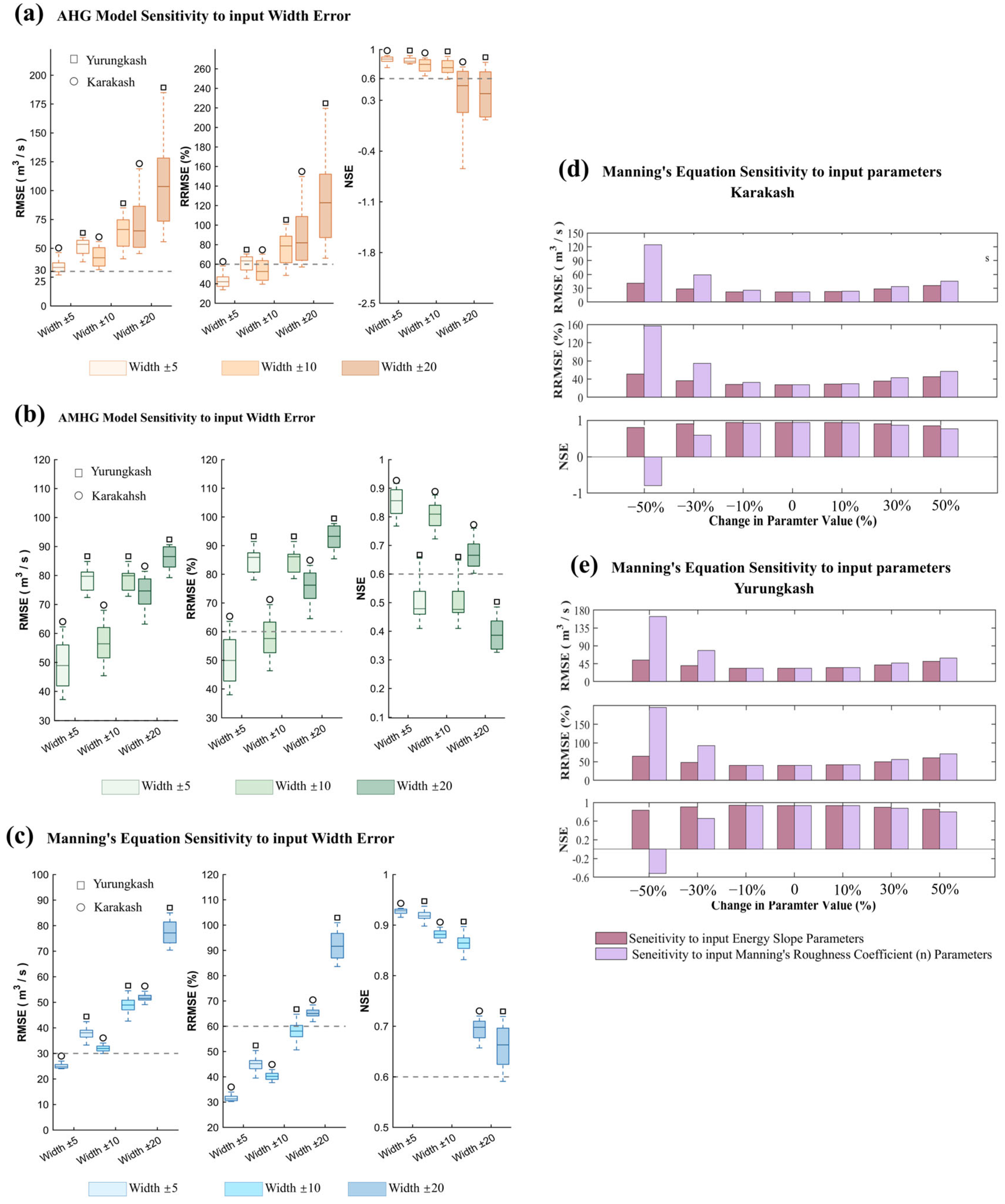
Although observational errors usually play a relatively minor role in the accuracy of discharge retrieval, which is typically dominated by errors in model parameters, their impact becomes amplified in narrower rivers [53,54]. Considering the influence of the spatial resolution of remote sensing imagery and systematic errors in water surface delineation on river width estimation, we introduced random errors of ±5 m, ±10 m, and ±20 m into the model based on a benchmark mean river width of 30 m and the spatial resolution of the imagery, as shown in Figure 6a–c. The results demonstrate that the Manning equation is less sensitive to river width errors than expected, showing superior robustness: its NSE remained above 0.6 across all error scenarios. In contrast, the accuracy of the single-year AHG model was more significantly affected by river width errors, with NSE declining by over 0.4 when errors exceeded ±10 m, leading to notable performance degradation. This stems from AHG being an empirical relationship between river width and discharge, where accuracy depends on the representativeness and sample size of calibration data, making discharge estimates more sensitive to input errors.

Conversely, the AMHG model relies on fewer parameters and shows minimal sensitivity to river width errors. With errors within ±10 m, the NSE of all three models decreased by only 0.09. The Yurungkash River exhibited higher sensitivity to width errors compared to the concurrently studied Karakash River, primarily due to its narrower channel. Overall, observational errors in river width had a limited impact on remote sensing discharge (RSQ), consistent with previous studies [39,46,47,50]. However, practical applications should account for inter-model variability.

In Manning-based discharge estimation, the roughness coefficient has a more pronounced effect on simulation results than the hydraulic slope, as shown in Figure 6d,e. Parameter perturbation experiments reveal that when the hydraulic slope deviates by more than 10%, the NSE rapidly deteriorates. Additionally, lower-roughness settings lead to a sharp increase in calculated flow velocity, consistent with the findings of Bjerklie et al. [54]. Overall, the AMHG model is less sensitive to river width errors than the other models.

4. Discussion

4.1. Reach Selection for Runoff Retrieval

Since geomorphology can influence discharge estimation, when selecting virtual station locations, study reaches should ideally be straight during both dry and wet seasons, with minimal variation in river width along the reach, and braided channels should be avoided. Higher channel sinuosity and steeper slopes complicate water surface slope variations from upstream to downstream, amplifying inherent errors in Manning’s equation for discharge estimation. In contrast, consistent channel geometry helps to reduce errors associated with the area–width method. Braided channels present challenges in remote sensing imagery due to blurry boundaries and dispersed water bodies, making it difficult to accurately extract the “effective river width.” Even if the width is extracted, the uneven distribution of flow among branches and significant cross-sectional variations often violate the mass conservation principle required for retrieval, leading to potential failures. Additionally, rectangular cross-sections and U-shape cross-sections should be avoided. When riverbanks are nearly vertical, increased runoff primarily results in deeper water rather than significant width changes. In such cases, original formulas based on width-dominated retrieval mechanisms are indeed no longer applicable. Sections with gentle channel slopes, where the variation in river width is significantly greater than the change in water depth, should be prioritized. Such sections typically exhibit a wide-shallow morphology in terms of hydraulic geometry, and their cross-sectional shapes can approximate trapezoidal, V-shaped, or arcuate forms.

4.2. Analysis of the Primary Sources of Error in Runoff Retrieval Accuracy

Previous research indicates that discharge retrieval accuracy is primarily influenced by model parameter errors, with observational errors playing a relatively minor role. However, the impact of observational errors is amplified in narrower rivers. Structural errors of the models themselves have the least influence on the results. Therefore, in practical applications, the impact of formula limitations on discharge estimation remains within an acceptable range [50,53]. River width observation error, one of the main errors in this study, has minimal impact on RSQ results, consistent with prior research [39,45,48,54]. However, differences between models should be considered in practical applications.

The vertical resolution of DEM data also affects discharge estimation using Manning’s equation, particularly in low-gradient rivers, where vertical DEM errors can cause significant variations in local slopes over short distances. Therefore, when calculating slopes, it is advisable to use the overall average slope of the entire study reach or a longer segment to smooth out “step noise” in elevation data, reducing the impact of the DEM’s vertical resolution errors and obtaining a more representative slope value. Future efforts should incorporate a higher-precision LiDAR DEM to mitigate this source of uncertainty.

4.3. Model Seasonal Variations and Regionalization Potential

Model performance varies by season, with better discharge estimation during high-flow periods and significant deviations during dry seasons, especially when the river width is less than 20 m. This is mainly due to the spatial resolution of remote sensing imagery and DEM data. In narrower channels, relative errors from resolution limitations become more pronounced. While model performance is generally better in wider channels, absolute errors still increase with higher discharge. However, although spatial resolution significantly affects dry-season discharge estimates, the impact on annual runoff overall remains acceptable since the aim of this study is to monitor long-term dynamic changes in rivers.

Furthermore, the AHG exponents demonstrate significant correlation and stability across both time and space. Parameters are highly similar across different years in the same river and even between different rivers. This may be attributed to erosion-resistant channel structures and dynamic equilibrium in sediment transport, maintaining long-term stability in channel geometry. The stability of the river’s longitudinal slope and bed composition further sustains this geomorphic equilibrium. Qin et al. (2020) also found minimal interannual variation in the AHG exponent b in mountainous rivers with erosion-resistant banks and stable channels [47], noting that the stability of the exponent b positively correlates with watershed area. The spatiotemporal stability and similarity of AHG parameters have important implications for hydrological regionalization and method transfer. When AHG parameters from the Yurungkash River were directly applied to the adjacent Karakash River, the model’s RRMSE increased by 22%, but the NSE remained at 0.80, indicating that the model explains 80% of the variance in observed data and accurately captures runoff dynamics. This result suggests that while direct transfer of AHG parameters between adjacent basins leads to some decline in simulation accuracy, this parameter transfer approach still holds practical value for water resource management, especially in scenarios not requiring high-precision retrieval. Particularly in neighboring basins lacking observed data, this regionalization method can provide feasible initial estimates for hydrological modeling.

4.4. Limitations and Future Improvement Pathways

Although the study demonstrates that the Manning equation, single-year AHG model, and width AMHG model can effectively estimate discharge in arid-region rivers, their performance during low-flow periods remains unsatisfactory due to observational and parametric uncertainties. The remote sensing images used in this study have a spatial resolution of 10–30 m. While data applicability was improved through image fusion techniques, the minimum resolution was only 10 m. During dry seasons, river channels often occupy just a single pixel in the imagery, significantly reducing the retrieval accuracy of all three models under such hydrological conditions.

Notably, this study treated the Manning coefficient as a constant, whereas in reality, it varies with river depth—particularly between flood and dry seasons [55]. Previous studies suggest that such variations can be expressed as logarithmic or power functions of relative depth [55]. However, due to the lack of in situ measurements, this dynamic coupling mechanism could not be incorporated into the computational framework.

Future research should leverage publicly available digital elevation models (DEMs) to derive prior cross-sectional channel data, then either:

(1) Represent the Manning coefficient’s depth-dependent variation via a continuous function, or

(2) Simplify the approach by dynamically adjusting the coefficient across different hydrological seasons to reduce systematic errors.

This refinement could significantly enhance model reliability, particularly for low-flow conditions.

5. Conclusions

Rivers in arid regions typically have a relatively small average width but exhibit extremely strong seasonal runoff variations and rapid discharge fluctuations. Previous studies have often identified arid regions as low-efficiency areas for discharge retrieval, with limited discussion on the adaptability of different models to such rivers [15,45,51]. This study systematically evaluates the applicability of three discharge retrieval techniques in arid-region rivers and has achieved breakthrough progress.

The key findings are as follows:

(1) The Manning equation demonstrated superior performance, particularly during high-flow periods, and was highly robust to river width errors, making it the preferred method for discharge retrieval in arid regions. The AHG model, capable of reconstructing long-term discharge series with minimal observed data, showed heightened sensitivity to river width errors and is best suited for scenarios with partial observational data. The AMHG model reduced reliance on ground data, enabling discharge estimation solely from river widths, but its accuracy suffered under strict constraints due to bias in the proxy variable $y$. Relaxing parameter optimization significantly improved its performance.

(2) The AHG exponent $\mathrm{b}$ in the study rivers displayed remarkable stability (coefficient of variation, suggesting that long-term discharge can be estimated with minimal calibration data in erosion-resistant channels. However, caution is needed when transferring parameters between adjacent basins, as direct application may increase errors.

(3) All models underperformed during low-flow periods, primarily due to limited remote sensing resolution and non-uniform flow in shallow channels. Future enhancements could integrate higher-resolution data or dynamic Manning coefficients to address these limitations.

(4) This study provides practical runoff monitoring tools for water resource management in arid regions, particularly for inland basins with sparse hydrological stations. Future work could leverage SWOT satellite data to improve narrow-river retrieval and explore regionalization patterns of AHG parameters to expand applicability.

References

1. Oki, T.; Kanae, S. Global Hydrological Cycles and World Water Resources. Science 2006, 313, 1068–1072. [Google Scholar] [CrossRef]
2. Deng, X.; Ye, A.; Tong, H. The Study of Measurement and Calculation Method on River Discharge. China Rural Water Hydropower 2015, 6, 18. (In Chinese) [Google Scholar]
3. Zhao, C.; Pan, X.; Yang, S.; Liu, C.; Chen, X.; Zhang, H.; Pan, T. Measuring Streamflow with Low-Altitude UAV Imagery. Acta Geogr. Sin. 2019, 74, 1392–1408. (In Chinese) [Google Scholar] [CrossRef]
4. Alsdorf, D.E.; Rodríguez, E.; Lettenmaier, D.P. Measuring Surface Water from Space. Rev. Geophys. 2007, 45, RG2002. [Google Scholar] [CrossRef]
5. Jiang, L.; Wu, H.; Lorenzo, A.; Li, X.; Kimball, J.S.; Chen, X. Review of Regionalization and Remote Sensing Based Method for Hydrological Model Parameters Calibration in Ungauged Basins. Acta Sci. Nat. Univ. Pekin. 2020, 56, 1152–1164. [Google Scholar]
6. Hannah, D.M.; Demuth, S.; van Lanen, H.A.J.; Looser, U.; Prudhomme, C.; Rees, G.; Stahl, K.; Tallaksen, L.M. Large-Scale River Flow Archives: Importance, Current Status and Future Needs. Hydrol. Process. 2011, 25, 5341–5352. [Google Scholar] [CrossRef]
7. Dinar, S. The Geographical Dimensions of Hydro-Politics: International Freshwater in the Middle East, North Africa, and Central Asia. Eurasian Geogr. Econ. 2012, 53, 115–142. [Google Scholar] [CrossRef]
8. Sun, W.; Wang, X.; Xu, Z. Estimating Streamflow Using Remote Sensing: Progress and Prospects. Acta Geogr. Sin. 2024, 79, 565–583. (In Chinese) [Google Scholar] [CrossRef]
9. Elmi, O.; Tourian, M.J.; Sneeuw, N. River discharge estimation using channel width from satellite imagery. In Proceedings of the 2015 IEEE International Geoscience and Remote Sensing Symposium (IGARSS), Milan, Italy, 26–31 July 2015; pp. 727–730. [Google Scholar] [CrossRef]
10. Du, B.; Jin, T.; Liu, D.; Wang, Y.; Wu, X. Accurate Discharge Estimation Based on River Widths of SWOT and Constrained At-Many-Stations Hydraulic Geometry. Remote Sens. 2023, 15, 1672. [Google Scholar] [CrossRef]
11. Wongchuig-Correa, S.; Paiva, R.C.D.D.; Biancamaria, S.; Collischonn, W. Assimilation of Future SWOT-Based River Elevations, Surface Extent Observations and Discharge Estimations into Uncertain Global Hydrological Models. J. Hydrol. 2020, 590, 125473. [Google Scholar] [CrossRef]
12. Domeneghetti, A.; Ceola, S.; Pugliese, A.; Persiano, S.; Palazzoli, I.; Castellarin, A.; Marinelli, A.; Brath, A. Potential Legacy of SWOT Mission for the Estimation of Flow-Duration Curves. Remote Sens. 2024, 16, 2607. [Google Scholar] [CrossRef]
13. Cui, B.; Gui, D.; Liu, Q.; Abd-Elmabod, S.K.; Liu, Y.; Lu, B. Distribution and Growth Drivers of Oases at a Global Scale. Earth’s Future 2024, 12, e2023EF004086. [Google Scholar] [CrossRef]
14. Gleason, C.J.; Durand, M.T. Remote Sensing of River Discharge: A Review and a Framing for the Discipline. Remote Sens. 2020, 12, 1107. [Google Scholar] [CrossRef]
15. Gleason, C.J.; Smith, L.C.; Lee, J. Retrieval of River Discharge Solely from Satellite Imagery and At-Many-Stations Hydraulic Geometry: Sensitivity to River Form and Optimization Parameters. Water Resour. Res. 2014, 50, 9614–9639. [Google Scholar] [CrossRef]
16. Hagemann, M.W.; Gleason, C.J.; Durand, M.T. BAM: Bayesian AMHG-Manning Inference of Discharge Using Remotely Sensed Stream Width, Slope, and Height. Water Resour. Res. 2017, 53, 9692–9707. [Google Scholar] [CrossRef]
17. Ran, L.; Wang, S.; Lu, X.X. Hydraulic Geometry Change of a Large River: A Case Study of the Upper Yellow River. Environ. Earth Sci. 2012, 66, 1247–1257. [Google Scholar] [CrossRef]
18. Sichangi, A.W.; Wang, L.; Yang, K.; Chen, D.; Wang, Z.; Li, X.; Zhou, J.; Liu, W.; Kuria, D. Estimating Continental River Basin Discharges Using Multiple Remote Sensing Data Sets. Remote Sens. Environ. 2016, 179, 36–53. [Google Scholar] [CrossRef]
19. Sichangi, A.W.; Wang, L.; Hu, Z. Estimation of River Discharge Solely from Remote-Sensing Derived Data: An Initial Study over the Yangtze River. Remote Sens. 2018, 10, 1385. [Google Scholar] [CrossRef]
20. Allen, G.H.; Pavelsky, T.M. Global Extent of Rivers and Streams. Science 2018, 361, 585–588. [Google Scholar] [CrossRef] [PubMed]
21. Yao, J.; Chen, Y.; Chen, J.; Zhao, Y.; Tuoliewubieke, D.; Li, J.; Yang, L.; Mao, W. Intensification of Extreme Precipitation in Arid Central Asia. J. Hydrol. 2021, 598, 125760. [Google Scholar] [CrossRef]
22. Chen, Y.; Li, B.; Li, Z.; Fan, Y.; Wang, H.; Deng, H. Water Resource Formation and Conversion and Water Security in Arid Region of Northwest China. J. Geogr. Sci. 2016, 26, 939–952. [Google Scholar] [CrossRef]
23. Chen, Y.; Li, Z.; Fan, Y.; Wang, H.; Deng, H. Progress and Prospects of Climate Change Impacts on Hydrology in the Arid Region of Northwest China. Environ. Res. 2015, 139, 11–19. [Google Scholar] [CrossRef]
24. Chen, Y. Water Resources Research in Northwest China; Springer: Dordrecht, The Netherlands, 2014. [Google Scholar] [CrossRef]
25. Yao, J.; Chen, Y.; Guan, X.; Zhao, Y.; Chen, J.; Mao, W. Recent Climate and Hydrological Changes in a Mountain-Basin System in Xinjiang, China. Earth-Sci. Rev. 2022, 226, 103957. [Google Scholar] [CrossRef]
26. Yao, J.; Chen, Y.; Zhao, Y.; Guan, X.; Mao, W.; Yang, L. Climatic and Associated Atmospheric Water Cycle Changes over the Xinjiang, China. J. Hydrol. 2020, 585, 124823. [Google Scholar] [CrossRef]
27. Chen, Y.; Zhu, C.; Li, Z.; Fa, G. High-quality development in the northern slope of the Kunlun Mountains: Issues, opportunities and challenges (in Chinese). Arid. Land Geogr. 2024, 47, 733–740. [Google Scholar] [CrossRef]
28. Li, Z.; Feng, Q.; Li, Z.; Yuan, R.; Gui, J. Climate Background, Fact and Hydrological Effect of Multiphase Water Transformation in Cold Regions of the Western China: A Review. Earth-Sci. Rev. 2019, 190, 33–57. [Google Scholar] [CrossRef]
29. Zhu, C.; Chen, Y.; Zhang, M.; Che, Y.; Sun, M.; Zhao, R.; Liu, Y. Preliminary Report on Scientific Investigation of Water Resources in the Northern Slope of Kunlun Mountains. Arid. Land Geogr. 2024, 47, 1097–1105. (In Chinese) [Google Scholar]
30. Han, X.; Chen, X. Analysis of Erosion and Deposition Characteristics of Hotan River Channel. Yellow River 2024, 46 (Suppl. S1), 26–28. (In Chinese) [Google Scholar]
31. Lanaras, C.; Bioucas-Dias, J.; Baltsavias, E.; Schindler, K. Super-Resolution of Multispectral Multiresolution Images from a Single Sensor. In Proceedings of the 2017 IEEE Conference on Computer Vision and Pattern Recognition Workshops (CVPRW), Honolulu, HI, USA, 21–26 July 2017; pp. 1505–1513. [Google Scholar] [CrossRef]
32. Ghimire, P.; Deng, L.; Nie, J. Effect of Image Fusion on Vegetation Index Quality—A Comparative Study from Gaofen-1, Gaofen-2, Gaofen-4, Landsat-8 OLI and MODIS Imagery. Remote Sens. 2020, 12, 1550. [Google Scholar] [CrossRef]
33. Al-Doski, J.; Hassan, F.M.; Norman, M.; Najim, A.A. Interaction of Image Fusion Techniques and Atmospheric Correction for Improve SVM Accuracy. Earth Sci. Inform. 2022, 15, 2673–2687. [Google Scholar] [CrossRef]
34. Li, H.; Zhao, J.; Yan, B.; Yue, L.; Wang, L. Global DEMs Vary from One to Another: An Evaluation of Newly Released Copernicus, NASA and AW3D30 DEM on Selected Terrains of China Using ICESat-2 Altimetry Data. Int. J. Digit. Earth 2022, 15, 1149–1168. [Google Scholar] [CrossRef]
35. Riggs, R.M.; Allen, G.H.; David, C.H.; Lin, P.; Pan, M.; Yang, X.; Gleason, C. RODEO: An Algorithm and Google Earth Engine Application for River Discharge Retrieval from Landsat. Environ. Model. Softw. 2022, 148, 105254. [Google Scholar] [CrossRef]
36. Li, D.; Wu, B.; Chen, B.; Xue, Y.; Zhang, Y. Review of Water Body Information Extraction Based on Satellite Remote Sensing. J. Tsinghua Univ. (Sci. Technol.) 2020, 60, 147–161. (In Chinese) [Google Scholar] [CrossRef]
37. Leopold, L.B.; Maddock, T., Jr. The Hydraulic Geometry of Stream Channels and Some Physiographic Implications; U.S. Geological Survey Professional Paper 252; U.S. Government Printing Office: Washington, DC, USA, 1953; p. 57. [CrossRef]
38. Alvarez Perez, A.B.; Grison, F.; Silva de Souza, K.I.; Borges Chaffe, P.L. Hydroclimatic Drivers of At-a-Station Hydraulic Geometry of Brazilian Rivers. J. Hydrol. 2024, 640, 131594. [Google Scholar] [CrossRef]
39. Sun, W.; Fan, J.; Wang, G.; Ishidaira, H.; Bastola, S.; Yu, J.; Fu, Y.H.; Kiem, A.S.; Zuo, D.; Xu, Z. Calibrating a Hydrological Model in a Regional River of the Qinghai–Tibet Plateau Using River Water Width Determined from High Spatial Resolution Satellite Images. Remote Sens. Environ. 2018, 214, 100–114. [Google Scholar] [CrossRef]
40. Gleason, C.J.; Wang, J. Theoretical Basis for At-Many-Stations Hydraulic Geometry. Geophys. Res. Lett. 2015, 42, 10327–10335. [Google Scholar] [CrossRef]
41. Gleason, C.J.; Smith, L.C. Toward Global Mapping of River Discharge Using Satellite Images and At-Many-Stations Hydraulic Geometry. Proc. Natl. Acad. Sci. USA 2014, 111, 4788–4791. [Google Scholar] [CrossRef] [PubMed]
42. Durga Rao, K.H.V.; Shravya, A.; Dadhwal, V.K. A Novel Method of Satellite-Based River Discharge Estimation Using River Hydraulic Geometry Through Genetic Algorithm Technique. J. Hydrol. 2020, 589, 125361. [Google Scholar] [CrossRef]
43. Bonnema, M.G.; Sikder, S.; Hossain, F.; Durand, M.; Gleason, C.J.; Bjerklie, D.M. Benchmarking Wide Swath Altimetry-Based River Discharge Estimation Algorithms for the Ganges River System. Water Resour. Res. 2016, 52, 8381–8397. [Google Scholar] [CrossRef]
44. McDowell, D.M. A General Formula for Estimation of the Rate of Transport of Non-Cohesive Bed-Load. J. Hydraul. Res. 1989, 27, 355–361. [Google Scholar] [CrossRef]
45. Lou, H.; Wang, P.; Yang, S.; Hao, F.; Ren, X.; Wang, Y.; Shi, L.; Wang, J.; Gong, T. Combining and comparing an unmanned aerial vehicle and multiple remote sensing satellites to calculate long-term river discharge in an ungauged water source region on the Tibetan Plateau. Remote Sens. 2020, 12, 2155. [Google Scholar] [CrossRef]
46. Zhang, W.; Wang, W.-G.; Zheng, J.-H.; Wang, H.-G.; Wang, G.; Zhang, J.-S. Reconstruction of Stage-Discharge Relationships and Analysis of Hydraulic Geometry Variations: The Case Study of the Pearl River Delta, China. Glob. Planet. Change 2015, 125, 60–70. [Google Scholar] [CrossRef]
47. Qin, C.; Wu, B.; Wang, Y.; Fu, X.; Xue, Y.; Li, D.; Li, M.; Zhang, Y. Dynamic Variability of At-a-Station Hydraulic-Geometry for Mountain Rivers in the Southeast Qinghai-Tibet Plateau: The Cases of Yalong River and Upper Jinsha River. CATENA 2020, 194, 104723. [Google Scholar] [CrossRef]
48. Hao, Z.; Xiang, N.; Cai, X.; Zhong, M.; Jin, J.; Du, Y.; Ling, F. Remote Sensing of River Discharge from Medium-Resolution Satellite Imagery Based on Deep Learning. Water Resour. Res. 2024, 60, e2023WR036880. [Google Scholar] [CrossRef]
49. Barber, C.A.; Gleason, C.J. Verifying the Prevalence, Properties, and Congruent Hydraulics of At-Many-Stations Hydraulic Geometry (AMHG) for Rivers in the Continental United States. J. Hydrol. 2018, 556, 625–633. [Google Scholar] [CrossRef]
50. Zhao, C.S.; Pan, X.; Yang, S.; Liu, C.; Chen, X.; Zhang, H.; Pan, T. Streamflow Calculation for Medium-to-Small Rivers in Data Scarce Inland Areas. Sci. Total Environ. 2019, 693, 133571. [Google Scholar] [CrossRef] [PubMed]
51. Lin, P.; Feng, D.; Gleason, C.J.; Pan, M.; Brinkerhoff, C.B.; Yang, X.; Beck, H.E.; Frasson, R.P.D.M. Inversion of River Discharge from Remotely Sensed River Widths: A Critical Assessment at Three-Thousand Global River Gauges. Remote Sens. Environ. 2023, 287, 113489. [Google Scholar] [CrossRef]
52. Kebede, M.G.; Wang, L.; Yang, K.; Chen, D.; Li, X.; Zeng, T.; Hu, Z. Discharge Estimates for Ungauged Rivers Flowing Over Complex High-Mountainous Regions Based Solely on Remote Sensing-Derived Datasets. Remote Sens. 2020, 12, 1064. [Google Scholar] [CrossRef]
53. Frasson, R.P.D.M.; Turmon, M.J.; Durand, M.T.; David, C.H. Estimating the Relative Impact of Measurement, Parameter, and Flow Law Errors on Discharge from the Surface Water and Ocean Topography Mission. J. Hydrometeorol. 2023, 24, 425–443. [Google Scholar] [CrossRef]
54. Bjerklie, D.M.; Durand, M.; Lenoir, J.; Dudley, R.W.; Birkett, C.M.; Jones, J.W.; Harlan, M. Satellite Remote Sensing of River Discharge: A Framework for Assessing the Accuracy of Discharge Estimates Made from Satellite Remote Sensing Observations. J. Appl. Remote Sens. 2023, 17, 014520. [Google Scholar] [CrossRef]
55. Ferguson, R. Flow Resistance Equations for Gravel- and Boulder-Bed Streams. Water Resour. Res. 2007, 43, W05427. [Google Scholar] [CrossRef]
Figure 1. The study area. (a) The location of the rivers on the northern slope of the Kunlun Mountains. (b) Spatial distribution of land use types, major rivers, hydrological stations, and river sections. (c) Elevation of the study area. (d) Interannual runoff variations in three representative rivers: the Karakash and Yurungkash Rivers (tributaries of the Hotan River, daily discharge data) and the Qarqan River (monthly discharge data).
Water 17 03105 g001
Figure 2. AHG Parameter Characteristics. (a,b) Power-law relationship. (c) Interannual variation. (d) Intra-annual fluctuation. (e) Interannual Parameter Correlations. (f) Intra-annual Parameter Relationships.
Water 17 03105 g002
Figure 3. AHG simulation results shown were calibrated using 2018 hydrometric station data, with other years serving as validation period. (a,b) Scatter plots and fitted curves of station discharge versus inverted discharge for the Karakash River. (c,d) Scatter plots and fitted curves of station discharge versus inverted discharge for the Yurungkash River.
Water 17 03105 g003
Figure 4. Application of the AMHG-GA Method in River Discharge Retrieval. (a) AMHG relationships, the purple dashed line represents the AMHG relationship between the Karakash and Yurungkash Rivers. (b) RS Slope relationships, the purple dashed line represents the RS Slope relationships between the Karakash and Yurungkash Rivers. (c,d) Comparison between gauged station discharge and simulated discharge. where Qrel mean: Discharge calculated using the mean of optimal parameter sets under relaxed AMHG constraints. Qre mid: Discharge calculated using the median of optimal parameter sets under relaxed AMHG constraints. Qstr mean: Discharge calculated using the mean of optimal parameter sets under strict AMHG constraints. Qstr mid: Discharge calculated using the median of optimal parameter sets under strict AMHG constraints. Q is the gauged discharge.
Water 17 03105 g004
Figure 5. Comparison between Manning-Strickle Equation estimated discharge and observed discharge. (a,b) Scatter plots with fitted rating curves for station discharge versus retrieval discharge in the Karakash River. (c,d) scatter plots with fitted rating curves for station discharge versus retrieval discharge in the Yurungkash River. (e) distribution of retrieval discharge for the Qarqan River, where the dark gray curve represents monthly mean discharge with shaded ranges of ±25% and ±50% daily discharge variability to assess temporal consistency between daily and monthly scales.
Water 17 03105 g005
Figure 6. Parameter Sensitivity Analysis. (ac) Sensitivity of different discharge retrieval models to input river width errors. (d,e) Sensitivity of Manning’s equation to variations in Manning’s n coefficient and hydraulic slope parameters.
Water 17 03105 g006