Deep Learning-Based Rolling Forecasting of Dissolved Oxygen in Shandong Peninsula Coastal Waters

Abstract

Changes in nearshore water quality directly influence ecosystem stability and the sustainability of aquaculture production. Among these factors, rapid fluctuations in dissolved oxygen (DO) can compromise the physiological functions of aquatic organisms, often leading to mass mortality events and significant economic losses. To enhance the predictive capability of DO in marine ranching areas, this study evaluates multiple forecasting approaches, including AutoARIMA, XGBoost, BlockRNN-LSTM, BlockRNN-GRU, TCN, Transformer, and an ensemble model that integrates these methods. Using hourly DO observations from coastal buoys, we performed multi-step rolling forecasts and systematically assessed model performance across multiple evaluation metrics (MAPE, RMSE, and R²), complemented by residual and error distribution analyses. The results show that the ensemble model, based on deep learning techniques, consistently outperforms individual models, achieving higher forecast robustness and more effective variance control, with MAPE values maintained below 4% across all three buoys. Building upon these findings, we further developed and deployed a DO forecasting and early-warning system centered on the ensemble framework. This system enables end-to-end functionality, including automatic data acquisition, real-time prediction, hypoxia risk identification, and alert dissemination. It has already been applied in marine ranching operations, providing 1–3 day forecasts of DO dynamics, facilitating the early detection of hypoxia risks, and significantly improving the scientific support and responsiveness of aquaculture management.

1. Introduction

Dissolved oxygen is a fundamental indicator of water quality and ecosystem stability. In nearshore marine ranching areas, abrupt declines in DO can induce stress responses in fish and shellfish, suppress feeding and growth, and even cause large-scale asphyxiation and mortality, leading to severe ecological and economic losses [1]. In recent years, DO levels in nearshore waters have exhibited a general declining trend, with hypoxic events occurring more frequently and posing direct threats to both ecosystems and cultured organisms. Strengthening the rapid and accurate forecasting of DO in marine ranching areas is therefore essential for the timely detection of potential hypoxia risks and the development of effective management strategies [2,3,4].

For the prediction and early warning of DO in nearshore aquaculture areas, early research primarily relied on physical models and statistical approaches, such as multiple linear regression (MLR), Autoregressive Integrated Moving Average (ARIMA), and Automatic Autoregressive Integrated Moving Average (AutoARIMA) [5,6], Although these methods are simple in structure and easy to interpret, they are limited in their ability to capture the nonlinear dynamics of DO. In recent years, researchers have increasingly applied machine learning approaches, such as support vector machines (SVM) [7], random forests (RF) [8], and extreme gradient boosting (XGBoost) [9], which have significantly improved the accuracy of single-step predictions. Some studies have further incorporated feature selection methods to enhance modeling efficiency [10].

To further enhance predictive performance, neural network-based deep learning methods have been extensively applied in DO forecasting, including multilayer perceptrons (MLP) [11], generalized regression neural networks (GRNN) [12], temporal models such as long short-term memory (LSTM) and gated recurrent units (GRU) [13,14], convolutional neural networks (CNN) [15], hybrid CNN-LSTM models [16], and, more recently, Transformer architectures [17]. Owing to their strong nonlinear representation and temporal memory capabilities, these models are particularly well suited to capturing the complex relationships between DO and factors such as temperature, salinity, and chlorophyll. They have already demonstrated promising results in DO prediction across diverse environments, including rivers, lakes, bays, and estuaries [18,19,20,21].

Several early-warning systems for dissolved oxygen (DO) monitoring have been developed in recent years. For instance, Xue et al. [22] designed a real-time DO prediction and warning system for carp aquaculture using neural-network and decision-tree models, enabling 10–60 min forecasts. Fakhrudin et al. [23] established an online stratification-based early-warning platform for Lake Maninjau, Indonesia, which continuously monitors temperature and DO profiles and issues SMS alerts before mass fish mortality events. More recently, Shaghaghi et al. [24] developed DOxy, an IoT- and machine-learning-based low-cost DO monitoring device capable of real-time sensing and threshold-based alerting, although it does not perform time-series forecasting. Anupama et al. [25] further combined random forest prediction with IoT sensors for river ecosystem management to enhance DO prediction accuracy. These studies provide valuable references for DO monitoring and risk management.

Although substantial progress has been made in DO prediction modeling, several key limitations remain. First, most existing studies rely on single models whose predictive accuracy is inherently limited when applied to complex and highly variable marine environments. Second, the capability for multi-step forecasting remains insufficient. Many models can only predict the next time point, offering very limited lead time for management actions. In real-world marine environmental regulation and aquaculture operations, it is crucial to forecast several hours or even days ahead to allow timely adjustment, water quality intervention, and disaster prevention. Third, although recent studies have begun to explore early-warning frameworks for hypoxia and water quality monitoring, most approaches remain model-centric, emphasizing prediction accuracy over the automated integration of real-time observations and early-warning mechanisms. With the growing availability of high-frequency buoy data, developing intelligent systems that combine real-time forecasting with dynamic alert generation has become increasingly important for effective marine environmental management.

To overcome these limitations, this study developed a multi-step DO forecasting framework based on nearshore buoy observations in the Shandong Peninsula. Unlike conventional single-model approaches, the proposed framework integrates multiple deep learning architectures within a unified structure to enhance predictive stability and accuracy in complex coastal environments. The model enables reliable 1–3 day DO forecasts, effectively addressing the limited lead time of traditional one-step prediction models. Furthermore, the optimized forecasting model was embedded into a near-real-time early-warning system, enabling automatic assimilation of buoy observations and dynamic alerts for potential hypoxia events, thereby providing proactive technical support for ecological protection and marine ranching management.

To provide a clear overview of the study design, Figure 1 presents the overall workflow of this research, including data acquisition, data preprocessing, model construction, forecasting, performance evaluation, and system construction.

2. Dataset Description and Preprocessing

2.1. Data Source

The marine environmental monitoring data used in this study were obtained from three coastal sites in the Shandong Peninsula, China—Laizhou Bay, Changdao, and Sanggou Bay—where buoys 0268, 0269, and 0270 were deployed, respectively. The geographical locations of these sites are shown in Figure 2, and the observed parameters, sampling frequency, observation depth, and regional information are summarized in

Table 1. Observation parameters, sampling frequency, and depth of each buoy.

Buoy ID	Area	Parameter	Unit	Frequency (min)	Depth (m)
0268	Laizhou Bay	Sea Temperature	°C	15	−3, −6
		DO	μmol/kg	30	−1
		Salinity	‰	15	−3, −6
		NN	mg/L	60	−1
		DOC	μmol/kg	60	−1
		Turbidity	NTU	30	−1
		Chl-a	RFU	30	−1
		CV	m/s	15	−2, −4, −6
		AP	hPa	15	2
		WS	m/s	15	2
		WH	m	15	−1

Note(s): DO—Dissolved Oxygen; Chl-a—Chlorophyll-a; DOC—Dissolved Organic Carbon; NN—Nitrate Nitrogen; CV—Current Velocity; AP—Air Pressure; WS—Wind Speed; WH—Wave Height.

. Due to deployment schedules and intermittent maintenance, the data coverage periods differed across buoys: buoy 0268 provided valid records from 10 November 2024 to 17 April 2025, buoy 0269 from 5 September 2024 to 12 May 2025, and buoy 0270 from 4 September 2024 to 30 April 2025.

Measurement depth: Positive values indicate sensor height above the sea surface (e.g., AP, WS), and negative values indicate depth below the sea surface (e.g., DO, CV, Chl-a).

2.2. Data Quality Control and Preprocessing

Prior to model training, the observational data from the three buoys were subjected to preprocessing and quality control to ensure the accuracy and physical consistency of the model inputs, thereby reducing the impact of sensor errors and anomalous fluctuations on the predictions.

2.2.1. Quality Control of Buoy Data

Since raw monitoring data often contain missing values, outliers, or sensor drift, directly using them for model training and prediction may impede model convergence and generalization, or even introduce significant biases. To address this, we designed a two-step quality control (QC) strategy: threshold-based QC and spike detection QC. In the threshold-based step, reasonable ranges were defined according to typical nearshore conditions (e.g., temperature 0–35 °C, salinity 15–40 PSU, dissolved oxygen 150–500 μmol/kg, chlorophyll 0–100 μg/L, nitrate nitrogen 0–5 mg/L, DOC 0–20 mg/L, current velocity 0–3 m/s, air pressure 950–1100 hPa, wind speed 0–25 m/s, wave height 0–5 m), thereby removing values that were clearly unrealistic or affected by sensor noise. On this basis, a spike detection method based on the 3σ (three-sigma) principle was applied [26], which identifies local anomalies by considering the differences between each observation and its neighboring values. The local rate of change is defined as:

$$\Delta t=max(\mid x_t-x_{t-1}\mid ,\mid x_t-x_{t+1}\mid )$$

(1)

Here, $\mid x_t-x_{t-1}\mid$ and $\mid x_t-x_{t+1}\mid$ represent the differences between the current observation and its preceding and succeeding values, respectively. To establish the threshold for spike detection, this study defined it based on the statistical characteristics of the differenced series:

$$\theta ={\mu }_d+k\times {\sigma }_d$$

(2)

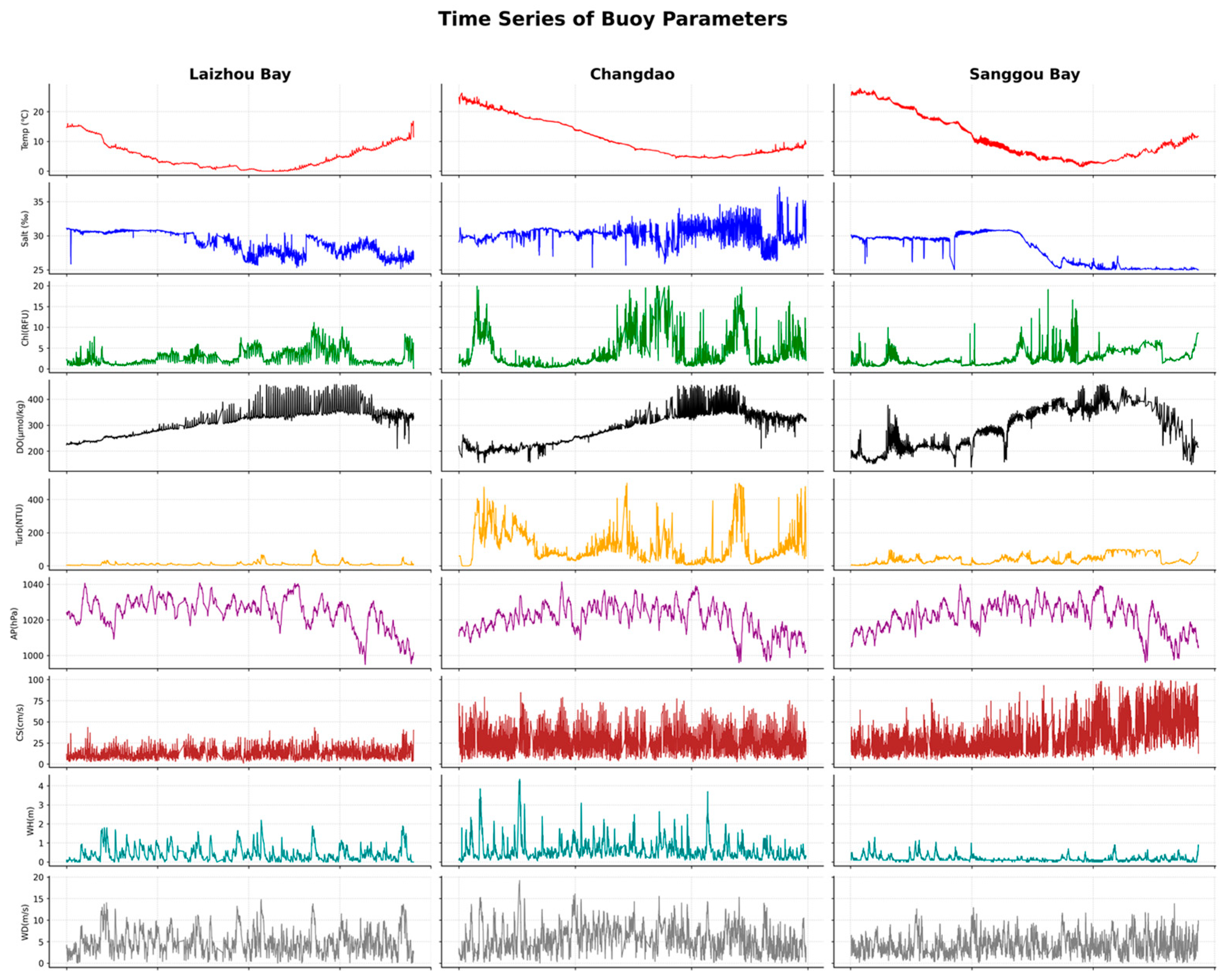
Here, ${\mu }_d$ and ${\sigma }_d$ denote the mean and standard deviation of the differenced series, respectively, and k is an empirical coefficient (set to 3 in this study). When ${\Delta }_t>\theta$, the point is identified as a spike anomaly and removed. The quality-controlled data from each buoy are shown in Figure 3.·

2.2.2. Data Preprocessing of Buoy Data

To ensure continuity in deep learning model predictions, missing values in the monitoring data were filled using linear interpolation for the target variable (dissolved oxygen) and its main covariates (temperature, salinity, and chlorophyll). This procedure removed temporal discontinuities caused by data gaps, thereby ensuring that the models received complete and continuous input sequences during training and forecasting. Furthermore, to harmonize the temporal resolution of different buoys and parameters and to facilitate subsequent sliding-window sample construction, all variables were resampled at 1 h intervals.

Since the parameters differ substantially in magnitude and units (e.g., temperature: 0–30 °C, salinity: 25–35, chlorophyll: 0–10 μg/L), directly feeding them into a neural network may lead to imbalanced gradient updates and hinder model convergence. To mitigate the effects of differing scales and value ranges, and to enhance the numerical stability and convergence speed of neural network training, this study applied min–max normalization to linearly rescale all variables into the [0, 1] range. The standard formula is:

$$X\prime ={\displaystyle \frac{X-X_{min}}{X_{max}-X_{min}}}$$

(3)

Here, $X$ denotes the original variable value, $X^{\prime }$ represents the normalized value within the range [0, 1], and $X_{min}$ and $X_{max}$ are the minimum and maximum values of the variable in the training samples, respectively.

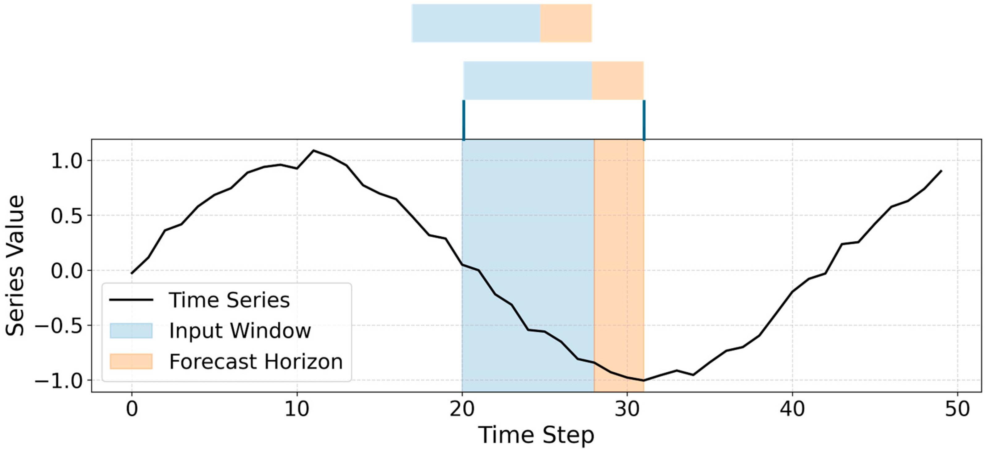
For sample partitioning, the data from each buoy were divided strictly in chronological order, with the first 70% used as the training set for parameter fitting and feature learning, and the remaining 30% reserved as the test set for validating rolling multi-step forecasts. During model training, a sliding-window strategy was employed to generate multi-step forecasting samples (Figure 4). Specifically, consecutive historical observations were segmented into fixed-length input windows, which were paired with the corresponding DO values over a future horizon to construct a large number of input–output pairs for model learning. This approach not only effectively captures the temporal dynamics of DO driven by multiple variables (e.g., temperature, salinity, chlorophyll), but also systematically augments the training dataset and enhances the model’s generalization capability across different temporal patterns.

In the testing phase, rolling forecasts were conducted on the reserved test sequences, simulating real-world applications in which future predictions are continuously generated from observed historical data. This design enabled a comprehensive evaluation of model stability and generalization performance across different forecasting horizons.

3. Model Construction

3.1. Covariate Selection for DO Forecasting

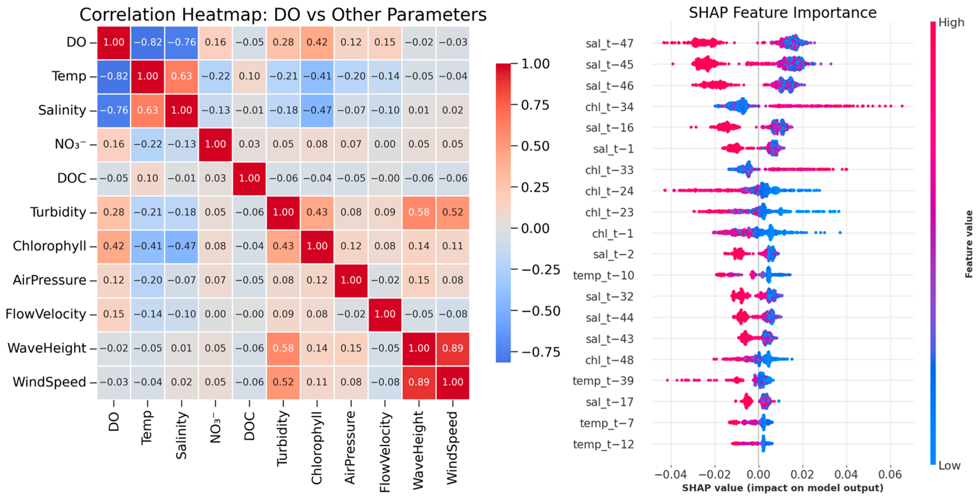
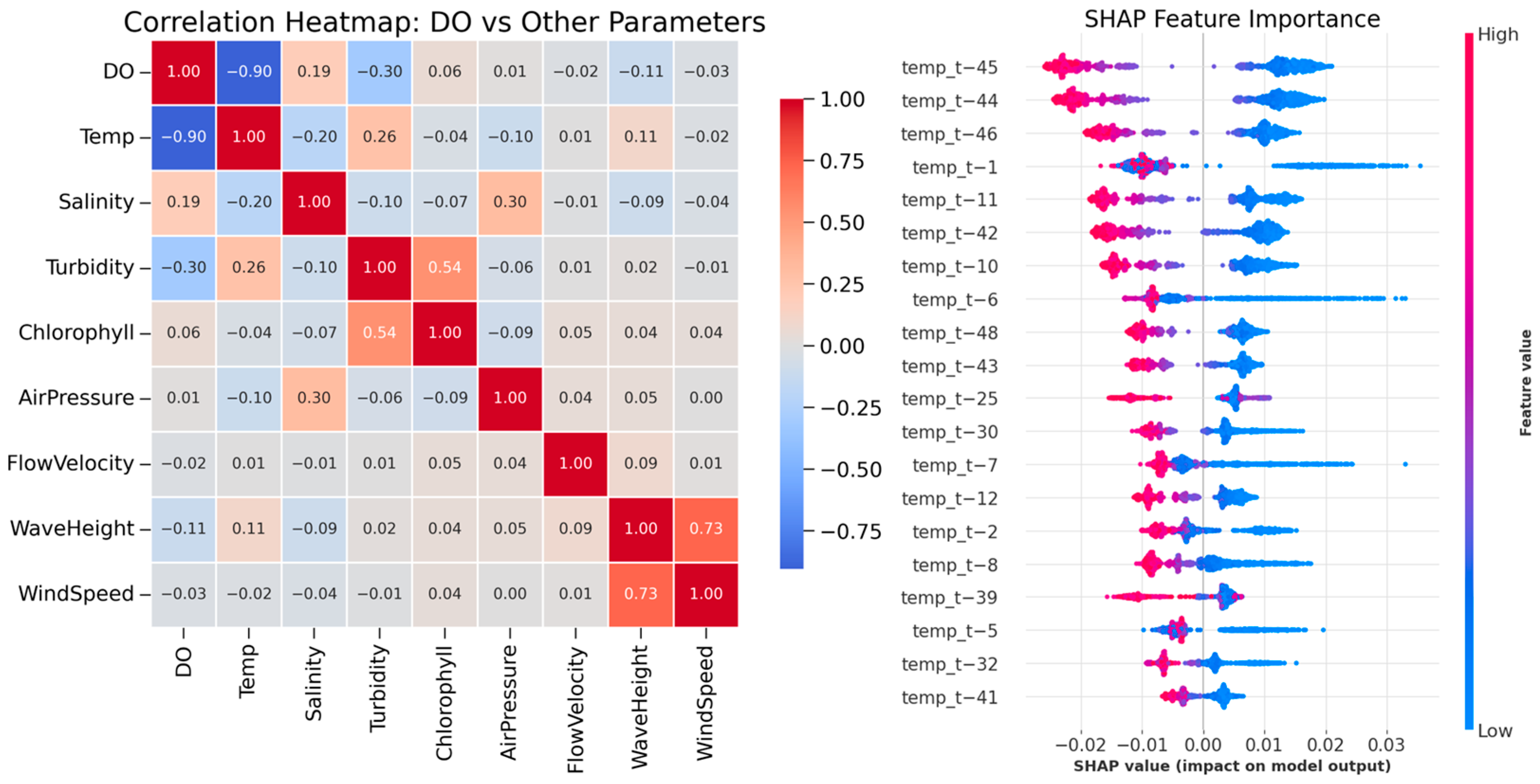
A comparative analysis of the Pearson correlation coefficients and the Shapley Additive Explanations (SHAP) results based on the Random Forest (RF) model for buoys 0268, 0269, and 0270 (Figure 5, Figure 6 and Figure 7) indicates that temperature consistently acts as the dominant controlling factor of DO. Across all three sites, temperature showed a strong negative correlation with DO (Pearson coefficients of approximately −0.8 to −0.9, with Spearman and MI indices showing similar patterns), confirming the robustness of this regulatory effect across regions. SHAP analysis further supported this finding, as multiple lagged temperature features (e.g., tempt-25, tempt-45) consistently ranked among the most influential predictors. These results demonstrate that temperature variations not only directly affect DO but also impose significant lagged effects, consistent with the physical mechanism by which elevated water temperature reduces oxygen solubility and gradually leads to DO depletion over time.

Salinity exhibited more heterogeneous effects across the three buoys. At buoys 0268 and 0270, salinity was moderately to strongly negatively correlated with DO (Pearson coefficients ranging from –0.66 to –0.76), with several lagged features contributing substantially in the SHAP analysis. This indicates that salinity variations in these regions play a non-negligible role in regulating DO, likely through indirect mechanisms associated with water mass exchange or mixing processes. By contrast, at buoy 0269, although salinity showed some statistical correlation with DO, its contribution to model predictions was negligible. This suggests that in this region, salinity may primarily represent long-term background variability rather than short-term dynamics.

Chlorophyll primarily reflected signals associated with biological processes. At buoys 0268 and 0270, chlorophyll exhibited a moderate positive correlation with DO (Pearson ≈ 0.4–0.5) and frequently appeared in the SHAP analysis as short-lag features (e.g., chl_t-1). This suggests that algal photosynthesis contributed to elevated DO concentrations, with effects typically manifested on short timescales. In contrast, at buoy 0269, chlorophyll displayed weak correlations and minimal predictive importance, likely due to stronger water exchange in this region, which may obscure biological signals.

Other environmental factors, including wind speed, current velocity, wave height, and air pressure, exhibited weak correlations with DO across all three buoys and contributed minimally in the SHAP analysis. This suggests that their direct influence on short-term DO variability is limited and may only become significant through indirect mechanisms or under extreme conditions.

Overall, the results demonstrate that temperature, salinity, and chlorophyll are the principal environmental drivers of DO variability in nearshore waters. Among them, temperature consistently showed strong dominance and pronounced lagged effects across all sites, making it the most stable controlling factor; salinity exerted a significant regulatory influence in certain regions, largely associated with hydrodynamic processes; and chlorophyll captured biological response signals on short timescales. Collectively, these physical (temperature, salinity) and biological (chlorophyll) drivers represent the primary mechanisms governing DO variability and were therefore identified as the key input factors for subsequent modeling.

3.2. Forecasting Model Architectures

In this study, seven representative time-series forecasting models were employed to perform 24-step multi-horizon predictions of surface DO concentrations based on buoy observations, and their performances were systematically compared. These models were selected to represent three major categories of forecasting approaches. The AutoARIMA model served as a classical statistical baseline for capturing linear temporal dependencies. XGBoost represented a machine-learning regression method capable of modeling nonlinear relationships between DO and environmental factors. The deep-learning architectures—BlockRNN-LSTM, BlockRNN-GRU, Temporal Convolutional Network (TCN), and Transformer—were employed to learn complex temporal dynamics through recurrent, convolutional, and attention mechanisms. Furthermore, a deep-learning ensemble model was developed by integrating the predictions of the four deep architectures to combine their complementary strengths and reduce the bias and variance inherent in individual models. The core structures and key hyperparameters of all models are summarized in

Table 2. Summary of the seven predictive models with core structures and key hyperparameters.

Model Category	Model Name	Core Structural Characteristics	Key Hyperparameters
Statistical	AutoARIMA	ARIMA with automatic order/seasonality selection	P = 5, q = 5, P = 2, Q = 2, m = 24, d = 1, D = 1
Machine Learning	XGBoost	Gradient-boosted decision trees	n_estimators = 100, max_depth = 6, learning_rate = 0.3, subsample = 0.8, colsample_bytree = 0.8, min_child_weight = 5
Deep Learning	BlockRNN-LSTM	Recurrent network with LSTM blocks (block-wise sequence modeling)	input_length = 144, output_length = 24, hidden_size = 32, n_layers = 3, dropout = 0.2, batch_size = 16
Deep Learning	BlockRNN-GRU	Recurrent network with GRU blocks (block-wise sequence modeling)	input_length = 144, output_length = 24, hidden_size = 64, n_layers = 2, dropout = 0.2, batch_size = 16
Deep Learning	TCN	Dilated causal 1D convolutions with residual/skip connections	input_length = 144, output_length = 24, kernel_size = 5, num_filters = 5, dilation = 2, dropout = 0.1
Deep Learning	Transformer	Self-attention encoder–decoder with causal masking	input_length = 96, output_length = 24, d_model = 16, n_heads = 4, n_layers = 2, ff_dim = 64, dropout = 0.1, batch_size = 16
Deep Learning	Ensemble (LSTM + GRU + TCN + Transformer)	Fusion of four deep nets (weighted averaging/stacking)	models = [GRUmodel, LSTMmodel, TCNmodel, Transmodel], fusion_strategy = NaiveEnsembleModel, weights = [0.25,0.25,0.25,0.25]

. Detailed explanations of the key hyperparameters listed in Table 2 are provided in Table S1.

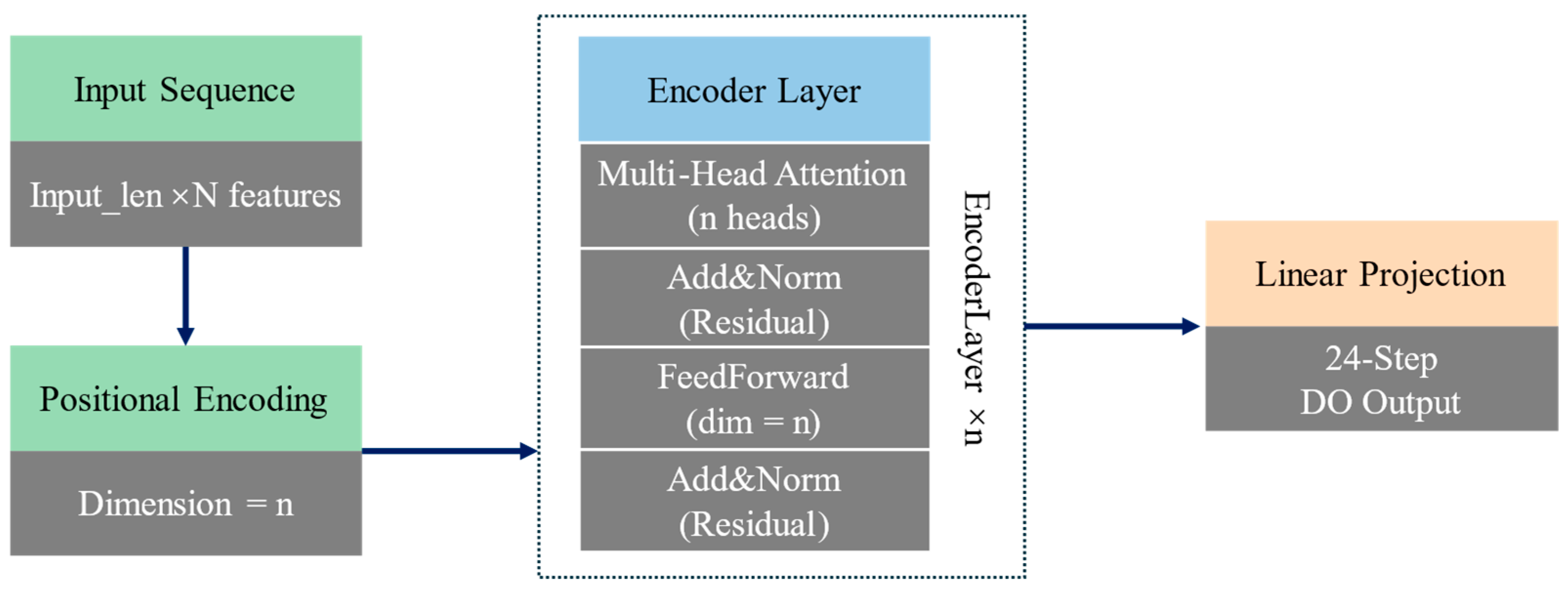
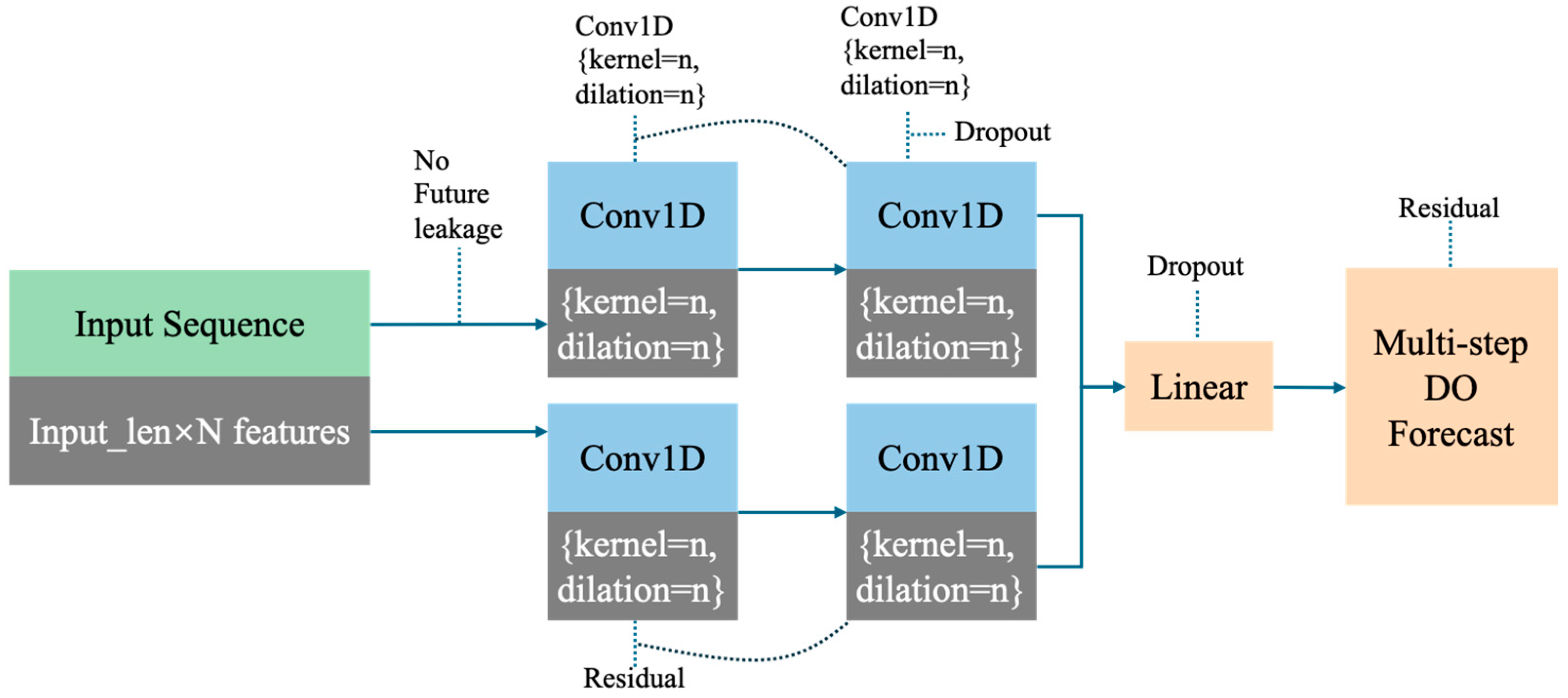
Among the deep learning models, TCN and Transformer are particularly representative. The former leverages dilated convolutions and residual structures to efficiently capture local and multi-scale temporal features, while the latter exploits self-attention mechanisms to model global dependencies and flexibly handle multivariate inputs. These two approaches thus represent two cutting-edge paradigms: “convolution-based local pattern modeling” and “attention-based global dependency modeling.” To illustrate their modeling logic, schematic diagrams of the two network structures are provided in Figure 8 and Figure 9. Detailed descriptions of the deep learning architectures (BlockRNN–LSTM, BlockRNN–GRU, and TCN) are provided in the Appendix A.

To enhance forecasting stability and accuracy, a deep-learning ensemble model was developed by integrating the predictions of four independently trained architectures: BlockRNN-LSTM, BlockRNN-GRU, TCN, and Transformer. These models capture complementary temporal characteristics—recurrent architectures (LSTM and GRU) are effective in modeling short- and medium-term dependencies, while convolutional (TCN) and attention-based (Transformer) networks better represent long-range temporal patterns. After individual training with optimized hyperparameters, their 24-step forecasts were aggregated using an equal-weight averaging scheme, which effectively reduces the bias and variance of individual models and enhances the robustness of multi-step dissolved oxygen forecasting under dynamic marine conditions.

Each model was trained and evaluated using hourly buoy observations. The input variables included DO, temperature, salinity, and chlorophyll. Among them, the AutoARIMA model performed univariate forecasting using only the DO time series (seasonal period m = 24), while all other models (XGBoost, BlockRNN-LSTM, BlockRNN-GRU, TCN, Transformer, and the ensemble) adopted a multivariate framework that combined DO with environmental covariates as inputs. The details are summarized in

Table 3. Input variables and lag configurations used in the forecasting models.

Model	Target Variable	Input Variables	Lag Range (hours)
AutoARIMA	DO	Time, DO	t-1~t-24
XGBoost	DO	Time, DO, Temp, Sal, Chl	t-1~t-72
BlockRNN-LSTM	DO	Time, DO, Temp, Sal, Chl	t-1~t-144
BlockRNN-GRU	DO	Time, DO, Temp, Sal, Chl	t-1~t-144
TCN	DO	Time, DO, Temp, Sal, Chl	t-1~t-144
Transformer	DO	Time, DO, Temp, Sal, Chl	t-1~t-144
EnsembleModel	DO	Time, DO, Temp, Sal, Chl	t-1~t-144

.

To ensure a fair comparison, all models were optimized and tested within a unified sliding-window backtesting framework. For XGBoost, key hyperparameters (n_estimators, max_depth, learning_rate) were tuned using the Optuna Bayesian optimization algorithm, which adaptively searches the parameter space based on previous evaluation results to efficiently find the best configuration. For the deep-learning models, major hyperparameters such as input_chunk_length, hidden_dim, batch_size, dropout, and n_epochs were optimized through grid search, a systematic trial of predefined parameter combinations to identify the one yielding the lowest validation error.

4. Results

We compared the forecasting accuracy of each model at the three nearshore buoy stations (0268, 0269, and 0270), with the results summarized in Table 3. The evaluation metrics included Mean Absolute Percentage Error (MAPE), Root Mean Squared Error (RMSE), and the coefficient of determination (R²), defined as follows:

$$\mathrm{MAPE}={\displaystyle \frac{100\%}{n}}{\sum }_{t=1}^n\left|{\displaystyle \frac{y_t-\widehat{y_t}}{y_t}}\right|$$

(4)

$$\mathrm{RMSE}=\sqrt{{\displaystyle \frac{1}{n}}{\sum }_{t=1}^n{\left(y_t-\widehat{y_t}\right)}^2}$$

(5)

$${\mathrm{R}}^2=1-{\displaystyle \frac{{\sum }_{t=1}^n{\left(y_t-\widehat{y_t}\right)}^2}{{\sum }_{t=1}^n{\left(y_t-\overline{y}\right)}^2}}$$

(6)

Here, $y_t$ denotes the observed value, $\widehat{y_t}$ the predicted value, $\overline{y}$ the mean of observations, and n the sample size. MAPE reflects the relative error level of the model, RMSE measures the absolute magnitude of prediction bias, and R² characterizes the model’s ability to explain the variance in the observations.

As shown in

Table 4. Comparison of rolling prediction errors for different models at multiple sites.

Buoy ID	Model	Train			Test
		Mape	RMSE (μmol/kg)	R2	Mape	RMSE (μmol/kg)	R2
0268	AutoArima	0.97%	6.171	0.98	6.02%	27.89	0.39
	XGBoost	2.21%	12.76	0.93	5.43%	28.05	0.39
	LSTM	1.37%	6.64	0.96	3.1%	16.28	0.79
	GRU	1.47%	5.97	0.97	3.09%	15.97	0.8
	Transformer	2.40%	10.66	0.95	2.53%	12.33	0.88
	TCN	1.4%	6.28	0.98	2.59%	13.59	0.86
	Essemble	1.01%	5.02	0.98	2.11%	11.01	0.9
0269	AutoArima	1.22%	5.66	0.98	5.48%	26.57	0.36
	XGBoost	3.34%	13.82	0.94	4.45%	21.88	0.57
	LSTM	2.71%	10.22	0.97	3.15%	14.87	0.8
	GRU	2.57	9.55	0.97	2.85%	13.44	0.83
	Transformer	2.86%	11.06	0.96	2.32%	10.83	0.89
	TCN	1.96%	7.49	0.98	3.03%	14.61	0.8
	Essemble	1.52%	5.81	0.98	2.06%	10.23	0.91
0270	AutoArima	2.06%	8.28	0.98	5.59%	23.11	0.89
	XGBoost	5.01%	19.89	0.93	6.65%	27.65	0.84
	LSTM	3.52%	12.89	0.97	4.35%	18.6	0.93
	GRU	3.64%	13.19	0.97	4.22%	17.9	0.93
	Transformer	4.74%	17.13	0.94	4.7%	19.9	0.92
	TCN	2.55%	9.55	0.98	4.14%	17.37	0.94
	Essemble	1.79%	6.48	0.98	3.7%	15.84	0.95

, the deep learning models (Transformer, LSTM, GRU, TCN) consistently outperformed both the statistical model (AutoARIMA) and the machine learning model (XGBoost). AutoARIMA exhibited persistently larger errors across stations (higher RMSE and lower R²), highlighting its limited capacity to capture the nonlinear dynamics of DO. By contrast, the deep learning models demonstrated stronger temporal modeling and fitting capabilities at all three sites. Overall, the ensemble forecasting model (Ensemble) achieved the highest predictive accuracy across stations, effectively improving accuracy while mitigating the instability observed in individual models.

To further examine whether the forecasting errors of different models were statistically different, a non-parametric Friedman test was applied to the absolute residuals derived from the rolling 24 h-ahead predictions on the test datasets for the three buoy stations (0268, 0269, and 0270). The Friedman test compares multiple related samples by ranking their errors and yields a chi-square (χ²) statistic and a corresponding p-value to assess the overall significance. The results revealed significant differences among models at all stations (χ² = 578.99–1745.71, p < 0.001), indicating that the forecasting errors were not drawn from the same distribution. Subsequently, pairwise Wilcoxon signed-rank tests with Holm correction for multiple comparisons were conducted to identify which models exhibited significantly lower forecasting errors. The post hoc analysis showed that the deep learning-based models (Transformer, TCN, BlockRNN-GRU, and BlockRNN-LSTM) and the ensemble model achieved significantly smaller errors than the traditional statistical (AutoARIMA) and machine-learning (XGBoost) models across all stations (adjusted p < 0.05).

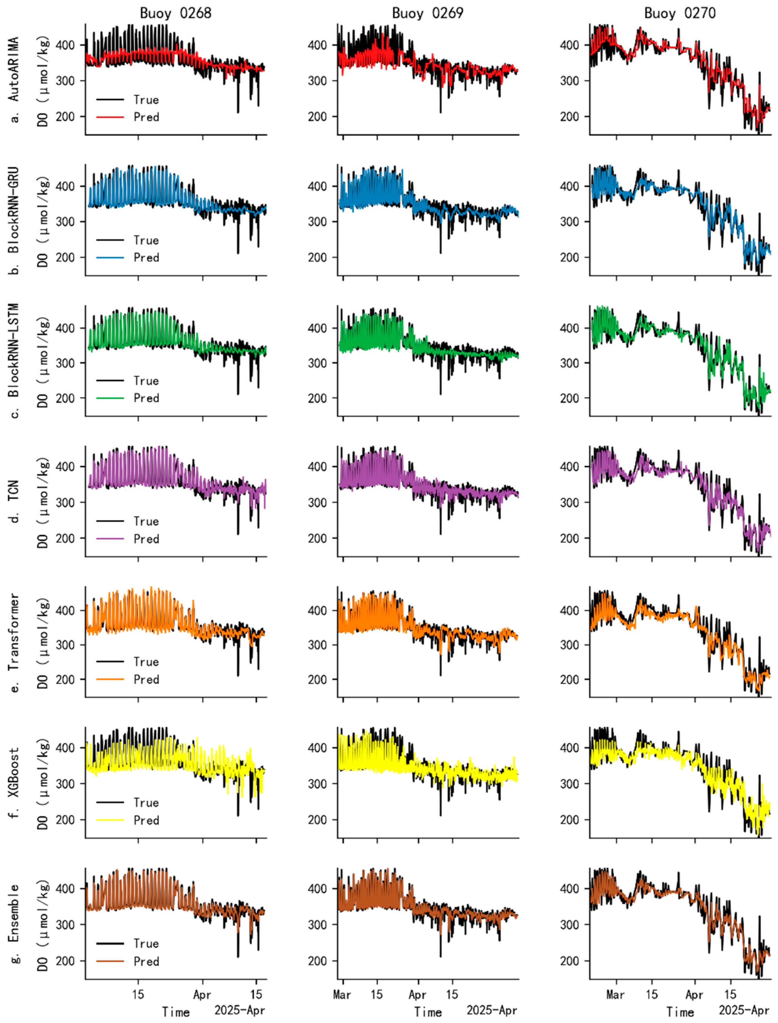
In addition, the time series plots of observed and predicted dissolved oxygen for all buoys and models on the testing dataset are presented in Figure 10. These visual comparisons further confirm the quantitative findings in Table 4, showing that the deep learning and ensemble models closely follow the temporal variations of measured DO, whereas the statistical and traditional machine learning models exhibit noticeable deviations during abrupt changes.

5. Discussion

5.1. Model Residual Analysis

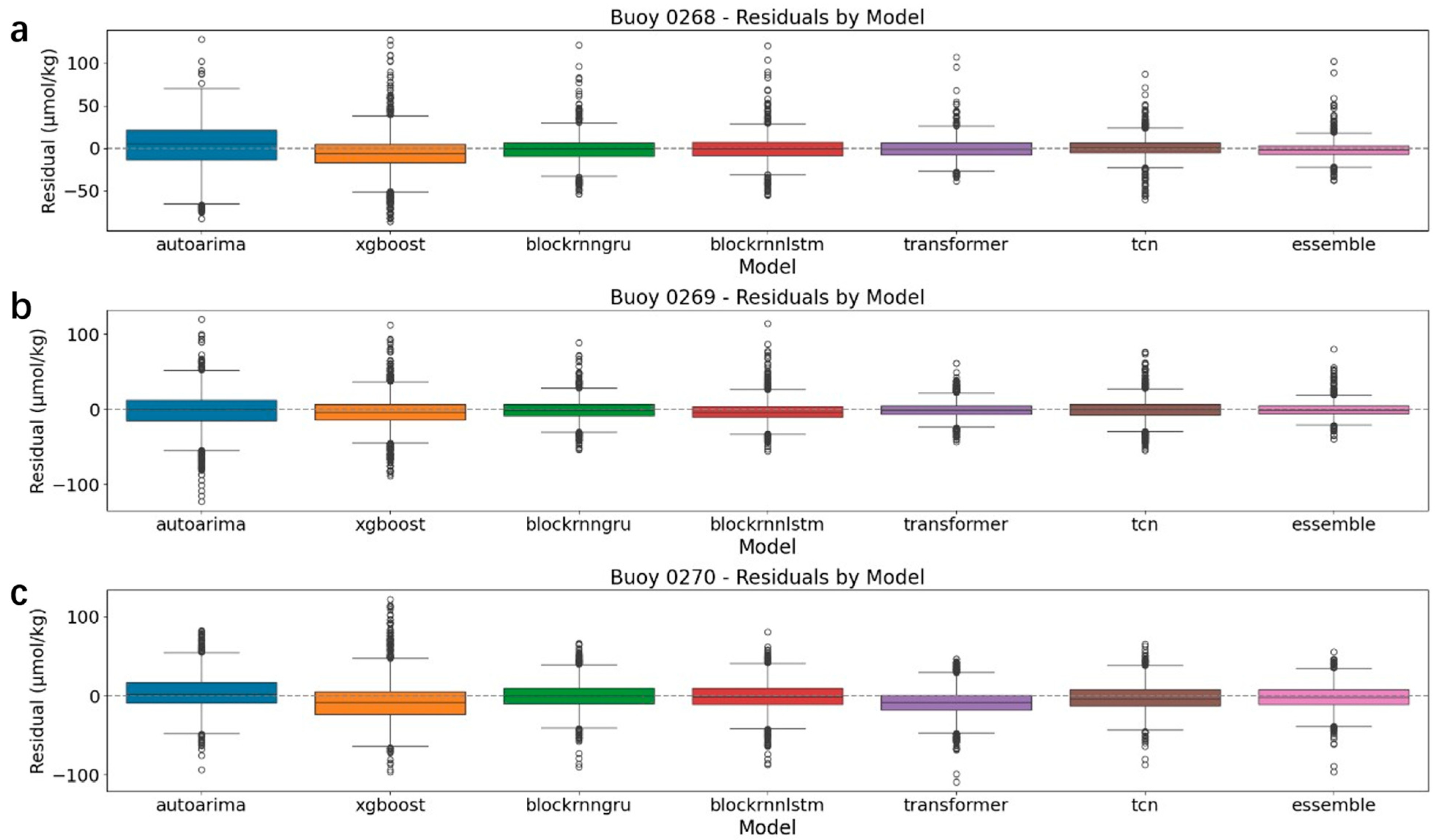
Figure 11 shows the residual distributions of different models at the three buoy stations. Overall, the ensemble forecasting model exhibited the most stable residual characteristics across all sites, with a median close to zero and the smallest dispersion, indicating strong robustness and unbiased performance. The deep learning models outperformed the statistical and machine learning methods, displaying smaller residual magnitudes and more concentrated distributions. By contrast, AutoARIMA and XGBoost exhibited wider residual fluctuations and more extreme values, highlighting their limited stability in prediction.

5.2. Evaluation of Ensemble Forecasting Models

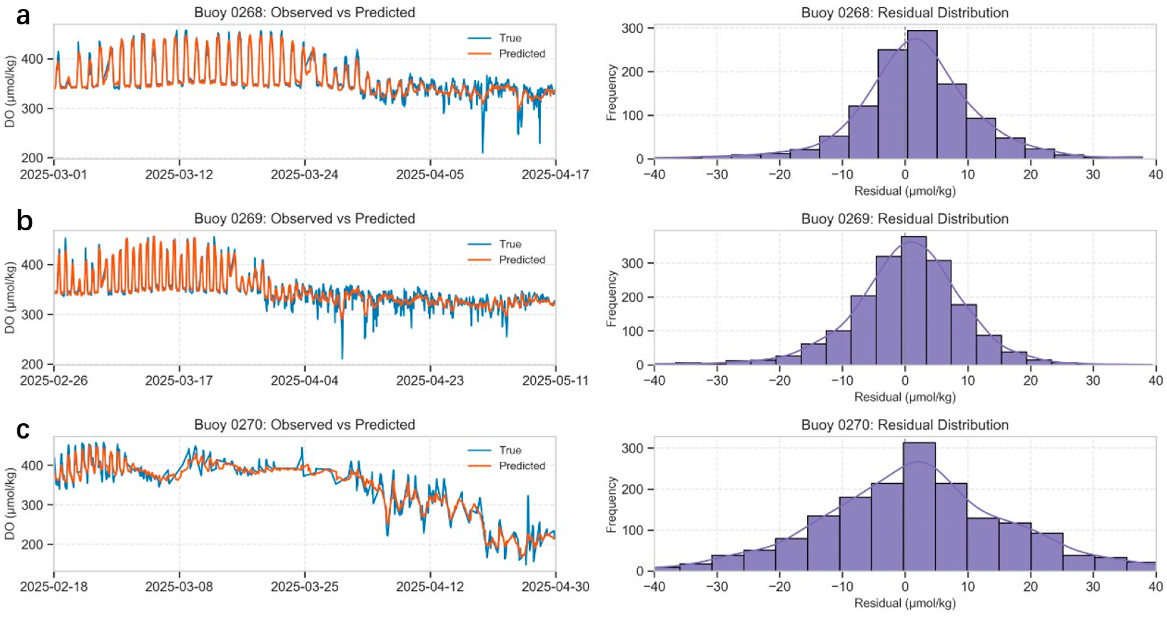
To further evaluate the performance of the ensemble forecasting model in multi-site DO prediction, Figure 12 presents its results at three representative buoys (0268, 0269, and 0270). For each buoy, the left panel displays a time-series comparison between observed and predicted DO values, while the right panel shows the histogram of prediction residuals (observation minus prediction). The time-series results demonstrate that the ensemble model accurately reproduces DO variation patterns at all three sites, effectively capturing both diurnal oscillations and abrupt changes. The residual distributions further reveal that prediction errors are largely concentrated within −20 to +20 μmol/kg, approximately following a normal distribution with mean values close to zero. This indicates that the model predictions are essentially unbiased and highly stable. Notably, despite the distinct geographical settings of the three buoys, the model consistently delivered stable and accurate forecasts across these spatially heterogeneous regions, highlighting its strong robustness.

Furthermore, the predictive uncertainty of the ensemble model was evaluated by calculating the standard deviation among the predicted values of its four submodels (GRU, LSTM, TCN, and Transformer) at each time step during the testing period, reflecting the inter-model spread rather than the residual variance. The mean inter-model standard deviations were 5.912 μmol/kg, 6.182 μmol/kg, and 7.536 μmol/kg for buoys 0268, 0269, and 0270, respectively, indicating generally low uncertainty and high stability of the ensemble forecasts across different sites.

Within the rolling forecasting framework, we evaluated the ensemble forecasting model using prediction horizons of 24, 48, and 72 h (

Table 5. Ensemble Model Error Across Forecast Horizons and Buoys (24/48/72 h).

Buoy ID	Forecast Horizon	MAPE	RMSE (μmol/kg)	R2
0268	24	2.11%	11.01	0.9
	48	2.43%	12.9	0.87
	72	2.83%	13.96	0.84
0269	24	2.06%	10.23	0.91
	48	2.47%	11.91	0.87
	72	2.71%	12.94	0.84
0270	24	3.7%	15.84	0.95
	48	3.85%	16.01	0.94
	72	4.17%	17.2	0.93

). The results show that the error levels under the three strategies are generally comparable and increase only slightly with longer horizons. R² remained stable across different horizons and stations, showing only minor declines as the forecast lengthened. This indicates that the model maintains stable and reproducible error characteristics within the 1–3 day forecasting range.

5.3. Comparison of Model Accuracy and Computational Efficiency for Each Buoy

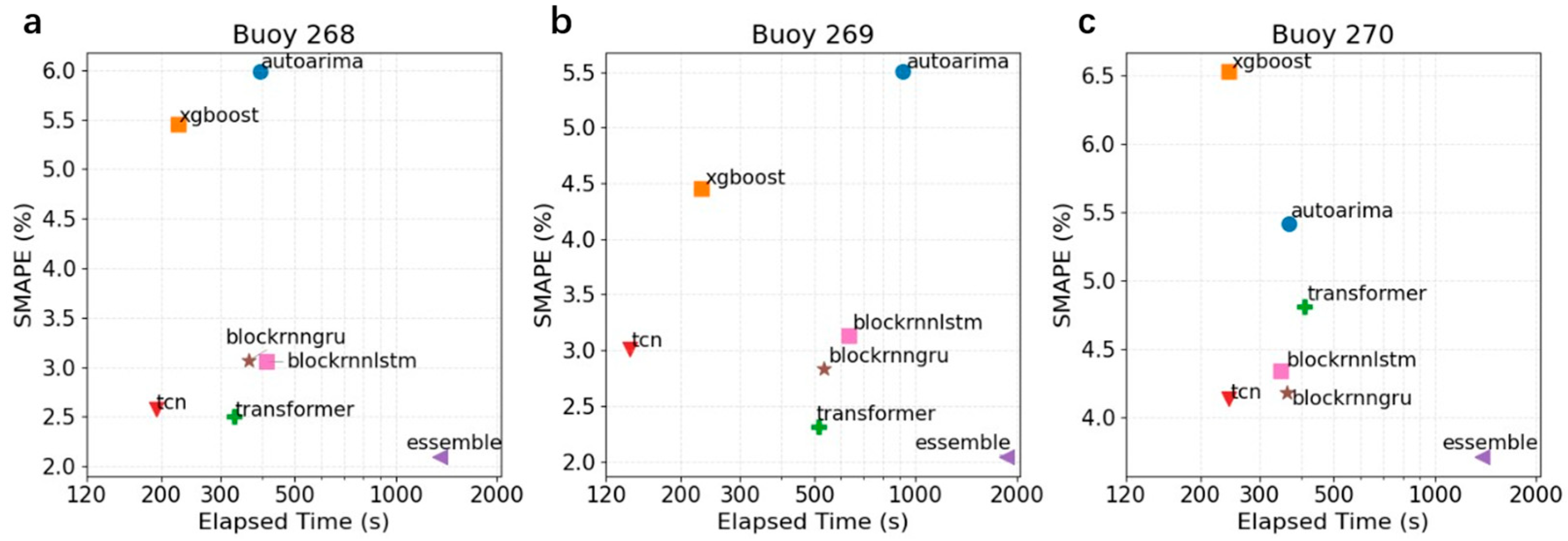
For comparison, the statistical model (AutoARIMA) was executed on a CPU, while all other models were trained and tested on an NVIDIA RTX 4070Ti GPU. Figure 13 compares the three buoys in terms of forecasting accuracy (SMAPE, %) and computational cost (seconds). The results show that the ensemble forecasting model achieved the lowest SMAPE (approximately 2–3%) across all stations, underscoring its clear advantage in accuracy, albeit with higher computational demand. This makes it more suitable for accuracy-oriented applications, such as environmental monitoring and hypoxia risk early warning in nearshore marine ranching. In contrast, AutoARIMA was both less accurate (SMAPE ≈ 5–6%) and relatively time-consuming, providing limited practical benefits. XGBoost, also CPU-based, offered faster computation but produced larger errors (SMAPE ≈ 5–6.5%), suggesting its value primarily as a rapid baseline. By comparison, the deep learning models executed on a GPU outperformed the traditional approaches overall. Among them, TCN stood out by maintaining relatively low SMAPE while achieving the shortest computation time, demonstrating excellent timeliness and making it particularly suitable for applications with stringent real-time requirements, such as factory-based recirculating aquaculture systems requiring immediate regulation.

5.4. Low-Oxygen Early-Warning System for Marine Ranching

Traditional environmental early-warning systems for marine ranching have mostly relied on numerical models to simulate hydrodynamic and ecological processes in order to anticipate potential hypoxia events. However, numerical models are often constrained by long computation cycles, complex deployment and maintenance, and limited capacity for real-time applications, which restrict their widespread use in nearshore aquaculture zones—particularly when responding to sudden hypoxic events.

To address these limitations, this study developed a hypoxia early-warning system tailored for marine ranching, based on buoy observations deployed in aquaculture waters. The system uses the Ensemble Regression model—identified in this study as the best-performing predictor—as its core, with key environmental factors such as temperature, salinity, and chlorophyll as input variables, to generate hourly forecasts of DO concentration up to 72 h in advance. Model execution supports GPU acceleration, ensuring high prediction accuracy while significantly reducing computational costs.

For effective early warning, two fixed ecological thresholds were incorporated into the system:

(1)

Ecological warning line (5 mg/L or 152 μmol/kg): Indicates the onset of mild hypoxia, where sensitive organisms may exhibit stress responses such as reduced feeding and metabolic activity. Enhanced monitoring and moderate adjustments in farming operations are recommended.

(2)

Hypoxia alert line (3 mg/L or 93 μmol/kg): Represents severe hypoxia levels, posing significant survival risks to cultured organisms. Immediate emergency interventions, such as oxygenation or water exchange, are advised.

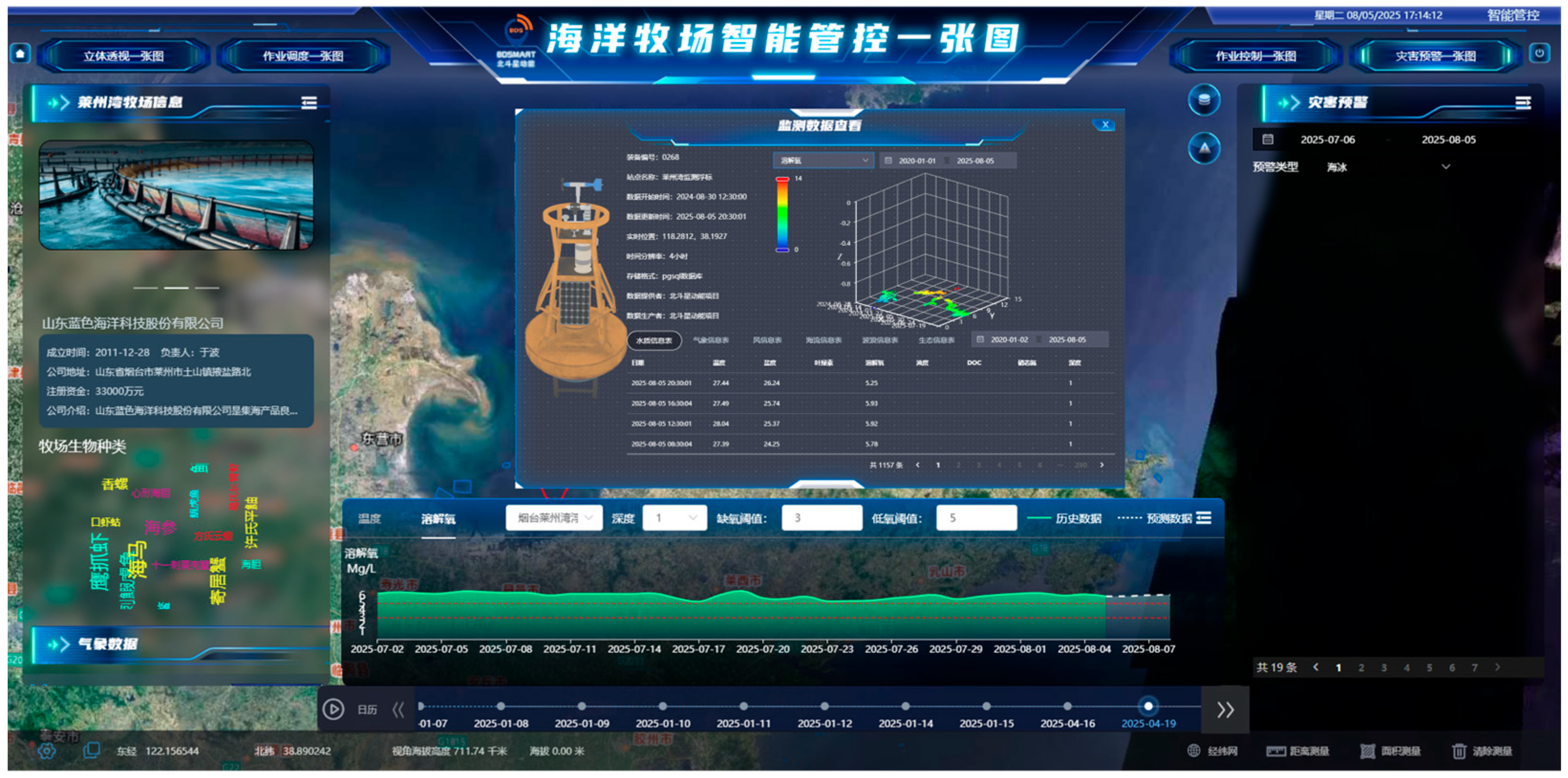
By applying these thresholds, the system automatically evaluates 72 h DO forecasts and cross-references predicted values below the alert line against an expert knowledge base to generate decision-support recommendations. The operational performance of the early-warning module was also examined. No false negatives were observed during the monitoring period, and a few false positives were mainly attributed to sensor drift or fouling, which caused abnormally low DO readings and led the model to generate underestimated forecasts. Figure 14 provides a schematic illustration of the decision-support early-warning system developed for Laizhou Bay.

6. Conclusions

This study systematically compared six single-model time-series forecasting methods—AutoARIMA, XGBoost, BlockRNN-LSTM, BlockRNN-GRU, TCN, and Transformer—for predicting dissolved oxygen (DO) from nearshore buoy observations.

A unified 24 h rolling forecasting framework was implemented across three buoy stations (0268, 0269, and 0270), and model performance was evaluated using MAPE, RMSE, and R² metrics. The comparison results show that deep learning models consistently outperform the traditional AutoARIMA and XGBoost methods. Among the single models, the Transformer and TCN architectures exhibited the most stable and accurate performance (MAPE ≈ 2.7%, RMSE ≈ 13–14 μmol kg⁻¹, R² ≈ 0.87–0.90), while the LSTM and GRU models demonstrated complementary temporal learning capabilities.

Based on these comparative findings and the structural complementarity among different deep learning models, this study further developed a multi-model ensemble forecasting framework that integrates the predictions of LSTM, GRU, TCN, and Transformer—representing the final proposed model of this work. This ensemble model further enhanced forecasting accuracy, achieving a mean MAPE of 2.6%, RMSE of 12.4 μmol kg⁻¹, and R² ≈ 0.92 across all sites—corresponding to an improvement of about 20–30% over the best single model and more than 50% over AutoARIMA.

Building on this framework, we deployed a near-real-time DO forecasting and early-warning system that provides a complete workflow from buoy data acquisition and real-time prediction to hypoxia risk identification and alert dissemination. The system has been successfully applied in marine ranching operations, providing reliable 1–3 day forecasts and issuing timely warnings before potential hypoxia events, thereby strengthening both scientific decision-making and emergency-response capability in aquaculture management.

References

1. Laffoley, D.; Baxter, J.M. Ocean Deoxygenation: Everyone’s Problem; IUCN: Gland, Switzerland, 2019; ISBN 978-2-8317-2014-2. [Google Scholar]
2. Gachloo, M.; Liu, Q.; Song, Y.; Wang, G.; Zhang, S.; Hall, N. Using Machine Learning Models for Short-Term Prediction of Dissolved Oxygen in a Microtidal Estuary. Water 2024, 16, 1998. [Google Scholar] [CrossRef]
3. Ahmed, A.A.M.; Jui, S.J.J.; Chowdhury, M.A.I.; Ahmed, O.; Sutradha, A. The Development of Dissolved Oxygen Forecast Model Using Hybrid Machine Learning Algorithm with Hydro-Meteorological Variables. Environ. Sci. Pollut. Res. 2023, 30, 7851–7873. [Google Scholar] [CrossRef]
4. Liang, X.; Jian, Z.; Tan, Z.; Dai, R.; Wang, H.; Wang, J.; Qiu, G.; Chang, M.; Li, T. Dissolved Oxygen Concentration Prediction in the Pearl River Estuary with Deep Learning for Driving Factors Identification: Temperature, pH, Conductivity, and Ammonia Nitrogen. Water 2024, 16, 3090. [Google Scholar] [CrossRef]
5. Moon, J.; Lee, J.; Lee, S.; Yun, H. Urban River Dissolved Oxygen Prediction Model Using Machine Learning. Water 2022, 14, 1899. [Google Scholar] [CrossRef]
6. Chen, C.-C.; Gong, G.-C.; Chou, W.-C.; Shiah, F.-K. Hypoxia in Autumn of the East China Sea. Mar. Pollut. Bull. 2020, 152, 110875. [Google Scholar] [CrossRef]
7. Garabaghi, F.H.; Benzer, S.; Benzer, R. Modeling Dissolved Oxygen Concentration Using Machine Learning Techniques with Dimensionality Reduction Approach. Environ. Monit. Assess. 2023, 195, 879. [Google Scholar] [CrossRef]
8. Abba, S.I.; Linh, N.T.T.; Abdullahi, J.; Ali, S.I.A.; Pham, Q.B.; Abdulkadir, R.A.; Costache, R.; Nam, V.T.; Anh, D.T. Hybrid Machine Learning Ensemble Techniques for Modeling Dissolved Oxygen Concentration. IEEE Access 2020, 8, 157218–157237. [Google Scholar] [CrossRef]
9. Granata, F.; Zhu, S.; Nunno, F.D. Dissolved Oxygen Forecasting in the Mississippi River: Advanced Ensemble Machine Learning Models. Environ. Sci. Adv. 2024, 3, 1537–1551. [Google Scholar] [CrossRef]
10. Li, W.; Fang, H.; Qin, G.; Tan, X.; Huang, Z.; Zeng, F.; Du, H.; Li, S. Concentration Estimation of Dissolved Oxygen in Pearl River Basin Using Input Variable Selection and Machine Learning Techniques. Sci. Total Environ. 2020, 731, 139099. [Google Scholar] [CrossRef] [PubMed]
11. Yang, J. Predicting Water Quality through Daily Concentration of Dissolved Oxygen Using Improved Artificial Intelligence. Sci. Rep. 2023, 13, 20370. [Google Scholar] [CrossRef]
12. Olyaie, E.; Zare Abyaneh, H.; Danandeh Mehr, A. A Comparative Analysis among Computational Intelligence Techniques for Dissolved Oxygen Prediction in Delaware River. Geosci. Front. 2017, 8, 517–527. [Google Scholar] [CrossRef]
13. Heddam, S. Intelligent Data Analytics Approaches for Predicting Dissolved Oxygen Concentration in River: Extremely Randomized Tree Versus Random Forest, MLPNN and MLR. In Intelligent Data Analytics for Decision-Support Systems in Hazard Mitigation: Theory and Practice of Hazard Mitigation; Deo, R.C., Samui, P., Kisi, O., Yaseen, Z.M., Eds.; Springer: Singapore, 2021; pp. 89–107. ISBN 978-981-15-5772-9. [Google Scholar]
14. Hu, Y.; Liu, C.; Wollheim, W.M. Prediction of Riverine Daily Minimum Dissolved Oxygen Concentrations Using Hybrid Deep Learning and Routine Hydrometeorological Data. Sci. Total Environ. 2024, 918, 170383. [Google Scholar] [CrossRef]
15. Wei, L.; Guan, L.; Qu, L. Prediction of Sea Surface Temperature in the South China Sea by Artificial Neural Networks. IEEE Geosci. Remote Sens. Lett. 2020, 17, 558–562. [Google Scholar] [CrossRef]
16. Liang, W.; Liu, T.; Wang, Y.; Jiao, J.J.; Gan, J.; He, D. Spatiotemporal-Aware Machine Learning Approaches for Dissolved Oxygen Prediction in Coastal Waters. Sci. Total Environ. 2023, 905, 167138. [Google Scholar] [CrossRef]
17. Chang, W.; Li, X.; Dong, H.; Wang, C.; Zhao, Z.; Wang, Y. Real-Time Prediction of Ocean Observation Data Based on Transformer Model. In Proceedings of the 2021 ACM International Conference on Intelligent Computing and Its Emerging Applications, Jinan, China, 28–29 December 2021; Association for Computing Machinery: New York, NY, USA, 2022; pp. 83–88. [Google Scholar]
18. Barzegar, R.; Aalami, M.T.; Adamowski, J. Short-Term Water Quality Variable Prediction Using a Hybrid CNN–LSTM Deep Learning Model. Stoch. Environ. Res. Risk Assess. 2020, 34, 415–433. [Google Scholar] [CrossRef]
19. Ayesha Jasmin, S.; Ramesh, P.; Tanveer, M. An Intelligent Framework for Prediction and Forecasting of Dissolved Oxygen Level and Biofloc Amount in a Shrimp Culture System Using Machine Learning Techniques. Expert Syst. Appl. 2022, 199, 117160. [Google Scholar] [CrossRef]
20. Ziyad Sami, B.F.; Latif, S.D.; Ahmed, A.N.; Chow, M.F.; Murti, M.A.; Suhendi, A.; Ziyad Sami, B.H.; Wong, J.K.; Birima, A.H.; El-Shafie, A. Machine Learning Algorithm as a Sustainable Tool for Dissolved Oxygen Prediction: A Case Study of Feitsui Reservoir, Taiwan. Sci. Rep. 2022, 12, 3649. [Google Scholar] [CrossRef]
21. Chen, X.; Zhao, C.; Chen, J.; Jiang, H.; Li, D.; Zhang, J.; Han, B.; Chen, S.; Wang, C. Water Quality Parameters-Based Prediction of Dissolved Oxygen in Estuaries Using Advanced Explainable Ensemble Machine Learning. J. Environ. Manag. 2025, 380, 125146. [Google Scholar] [CrossRef]
22. Xue, H.; Wang, L.; Li, D. Design and Development of Dissolved Oxygen Real-Time Prediction and Early Warning System for Brocaded Carp Aquaculture. In Proceedings of the Computer and Computing Technologies in Agriculture VI; Li, D., Chen, Y., Eds.; Springer: Berlin/Heidelberg, Germany, 2013; pp. 35–42. [Google Scholar]
23. Fakhrudin, M.; Subehi, L.; Jasalesmana, T.; Dianto, A. Dissolved Oxygen and Temperature Stratification Analysis for Early Warning System Development in Preventing Mass Mortality of Fish in Lake Maninjau, West Sumatera-Indonesia. IOP Conf. Ser. Earth Environ. Sci. 2019, 380, 012002. [Google Scholar] [CrossRef]
24. Shaghaghi, N.; Fazlollahi, F.; Shrivastav, T.; Graham, A.; Mayer, J.; Liu, B.; Jiang, G.; Govindaraju, N.; Garg, S.; Dunigan, K.; et al. DOxy: A Dissolved Oxygen Monitoring System. Sensors 2024, 24, 3253. [Google Scholar] [CrossRef]
25. Anupama, P.; Kumar, E.V.; Ajanth, S.; Anugna, K.; Venkatesh, J. ML-Based Predicting of Dissolved Oxygen Levels for Sustainable River Ecosystem Management. J. Sci. Eng. Technol. Manag. Sci. 2025, 2, 590–601. [Google Scholar] [CrossRef]
26. Li, S.; Wang, B.; Deng, Z.; Wu, B.; Zhu, X.; Chen, Z. Data Quality Control Method of a New Drifting Observation Technology Named Drifting Air-Sea Interface Buoy. J. Ocean Univ. China 2024, 23, 11–22. [Google Scholar] [CrossRef]
Figure 1. Overall workflow and framework of the dissolved oxygen forecasting study.
Water 17 03102 g001
Figure 2. Spatial distribution of buoy locations.
Water 17 03102 g002
Figure 3. Time series of key environmental parameters at each buoy station after quality control Colored lines represent different variables: red line for temperature, blue line for salinity, green line for chlorophyll, black line for dissolved oxygen, yellow line for turbidity, purple line for air pressure, dark red line for current velocity, cyan-green line for wave height, and gray line for wind speed.
Water 17 03102 g003
Figure 4. Illustration of the Sliding Window Strategy.
Water 17 03102 g004
Figure 5. Multivariate Correlation and SHAP Analysis—Buoy 0268.
Water 17 03102 g005
Figure 6. Multivariate Correlation and SHAP Analysis—Buoy 0269.
Water 17 03102 g006
Figure 7. Multivariate Correlation and SHAP Analysis—Buoy 0270.
Water 17 03102 g007
Figure 8. Schematic diagram of the Transformer model architecture.
Water 17 03102 g008
Figure 9. Schematic diagram of the TCN model architecture.
Water 17 03102 g009
Figure 10. Time series comparison between observed and predicted dissolved oxygen concentrations on the testing dataset at all buoy stations using different models: (a) AutoARIMA, (b) BlockRNN-GRU, (c) BlockRNN-LSTM, (d) TCN, (e) Transformer, (f) XGBoost, and (g) Ensemble.
Water 17 03102 g010
Figure 11. Residual distributions of seven models at three buoy stations: (a) Buoy 0268, (b) Buoy 0269, and (c) Buoy 0270. Boxplots display the median (center line), interquartile range (box), and extreme values (whiskers and outliers).
Water 17 03102 g011
Figure 12. Ensemble model results at three buoy stations: (a) Forecast curves and residual distributions for Buoy 0268, (b) Buoy 0269, and (c) Buoy 0270.
Water 17 03102 g012
Figure 13. Trade-off between prediction accuracy and computational efficiency for seven models at three buoy stations: (a) Buoy 0268, (b) Buoy 0269, and (c) Buoy 0270. The x-axis denotes the elapsed training and forecasting time (s), while the y-axis shows the Symmetric Mean Absolute Percentage Error (SMAPE, %).
Water 17 03102 g013
Figure 14. Prototype of the dissolved oxygen (DO) forecasting and early-warning system developed in this study. The left panel shows the basic introduction of the marine ranching area; the central part displays the buoy observation data, with the lower section showing the observation line, prediction line, and warning line of the early-warning system; the right panel illustrates the types of potential disasters.
Water 17 03102 g014