Optimizing Parameters of Marine Hydrodynamic Models Based on AFS Theory and PCA

Abstract

The parameter optimization of marine hydrodynamic models currently relies predominantly on expert empirical knowledge, but the quantitative indicators and weighting mechanisms for rapid calibration remain unclear due to inherent model uncertainties and complexities. This study addresses these challenges through expert questionnaires that collect fuzzy evaluations of calibration criteria, developing an integrated methodology combining the theory of axiomatic fuzzy set (AFS) with principal component analysis (PCA). Numerical case studies quantify calibration indicator weights and assess critical parameter impacts, revealing that bathymetry and roughness coefficients predominantly govern simulation accuracy. Elevated roughness conditions demonstrate two regimes: (1) at 1–2 × baseline roughness, strong positive correlations (with a coefficient of determination R² increased by up to 0.568 compared to baseline) confirm effective model-data matching for tidal levels/currents; (2) beyond 2 × baseline roughness, progressive correlation decay accompanies increasing coefficients, indicating amplified simulation–measurement discrepancies. Notably, under reduced roughness conditions, high accuracy persists during spring/mid-tide phases but significantly diminishes during neap tides, demonstrating enhanced roughness sensitivity in low-tidal energy regimes.

1. Introduction

The intensification of marine pollution has accelerated the advancement of numerical simulation studies of pollutant dispersion. The parameter optimization of marine hydrodynamic models, which is critical for improving simulation efficiency and accuracy, has emerged as a central scientific challenge in this domain [1,2,3]. To improve hydrodynamic model accuracy, several researchers have developed optimization approaches. Ref. [4] realizes model dynamic calibration via quantitative comparison and iteration of measured tidal current data and simulation results. Ref. [5] simplifies model parameters using a genetic algorithm, providing a theoretical optimization scheme for marine system forecasting, and Ref. [6] applies an evolutionary algorithm to a regional tidal model to optimize boundary conditions and physical parameters collaboratively. In [7], the author uses a hybrid genetic algorithm to find the optimal parameters of a coastal current model.

To achieve accurate and efficient calibration of marine hydrodynamic models, two critical tasks must be addressed: defining calibration metrics and determining their weighting. Researchers have systematically investigated various factors that influence the accuracy of hydrodynamic simulations, with shoreline configuration and bathymetry being the most extensively studied parameters. Ref. [8] found that coastal line changes directly alter the eroded sediment entering estuaries, thereby affecting the marine hydrodynamic flow field. Ref. [9] developed a 3D hydrodynamic model using Delft3D to analyze shoreline and depth variation effects on regional hydrodynamics in the Bohai Sea under pre- and post-reclamation conditions. In Ref. [10], MIKE21 was employed to assess 50-year shoreline evolution impacts on tidal currents, tidal prism, and water exchange in Laizhou Bay. Ref. [11] numerically simulated terrain erosion and deposition near Dongcun (southern Liugong Island) and found that terrain effectively alters hydrodynamic energy between coastal tides and spur dikes. Ref. [12] studied the effects of water depth and shoreline on tides and tidal currents in Liaodong Bay based on the Finite Volume Community Ocean Model (FVCOM) model. In Ref. [13], FVCOM revealed that shoreline morphology and depth variations regulate tidal amplitudes; in Ref. [14], FVCOM was used to evaluate hydrodynamic changes (tidal prism, currents and exchange rates) in Jiaozhou Bay under temporally varying shoreline/depth conditions. Ref. [15] explored the effect of shoreline changes in Jiaozhou Bay on water exchange based on MIKE. In Ref. [16], ROMS was applied to study M2 tidal constituent responses to shoreline and depth changes in the Yellow River Estuary and adjacent waters.

Research has also addressed tidal and wind field influences on flow dynamics. Ref. [17] studied wind’s impact on water exchange via 3D hydrodynamics theory, while Ref. [18] analyzed the synergistic effect of winter tides and wind fields in the Bohai Sea, incorporating tides, wind fields and temperature. Ref. [19] examined winter circulation formation mechanism in the Bohai Sea, considering wind stress distribution, tides and open-boundary inflow. Ref. [20] identified significant monsoon effects on Beibu Gulf circulation and anticyclonic eddies via FVCOM, and Ref. [21] examined monsoon–tide interactions governing tritium transport in Haizhou Bay (Yellow Sea). In Ref. [22], winter-wind-driven circulation velocity enhancement in the Bohai Sea was quantified using ROMS. Ref. [23] analyzed POM-based wind impacts on residual currents in Daya Bay. Ref. [24] evaluated storm wind disturbances to water exchange in Jiaozhou Bay, and Ref. [25] validated wind directional modulation of flow/residual fields in Laizhou Bay with Mike21FM. Ref. [26] demonstrated the effect of combined tide–eddy–wind forcing on South China Sea bottom circulation. In Refs. [27,28], FVCOM was used to simulate tidal–wind–runoff coupling in Pearl River Estuary inner-bay exchange, and Ref. [29] investigated tidal dominance in regional hydrodynamic environments.

The roughness coefficient (bottom friction coefficient) is a critical calibration and validation parameter for hydrodynamic models. Ref. [30] emphasized the influence of different bottom friction coefficients on tides, tidal currents and residual currents in the Beibu Gulf. Ref. [31] replicated tidal bore dynamics by refining seabed friction coefficients, and Ref. [32] developed a terrain-dependent roughness calculation method that enhanced simulation accuracy. Ref. [33] quantified bottom friction effects on bay surface elevation and velocity amplitudes. In Ref. [34], M2 tidal constituent simulations in the Bohai–Yellow–East China Seas were improved by optimizing friction coefficients under fixed boundary conditions. Ref. [35] introduced genetic algorithm-driven roughness inversion for hydrodynamic model calibration.

Temperature–salinity effects on flow fields have also been investigated. Ref. [36] compared differences between tidal residual currents, wind-driven currents and thermohaline currents based on the 3D ECOMSED model. Ref. [37] developed a hydrodynamic and thermal–salinity model for the Bohai Sea with the MIKE3 Flow Model, assessing wind, precipitation and evaporation impacts. Ref. [38] constructed a 3D tidal current and thermal–salinity model for Xiangshan Harbor using FVCOM, integrating tidal currents, wind, solar radiation and runoff.

In summary, key factors affecting hydrodynamic model accuracy encompass shoreline, water depth, tides, wind fields, temperature–salinity and roughness. However, three-dimensional marine hydrodynamic model calibration still faces challenges including diverse numerical schemes, inconsistent calibration methods and excessive reliance on expert experience, with no systematic calibration framework established.

Determining calibration indicator weights remains critical. While the Delphi method and Analytic Hierarchy Process (AHP) are widely adopted, both exhibit limitations. The Delphi method requires experts to quantify subjective judgments, but weight determination relies on personal experience with limited objectivity; it also neglects opinion disparities by averaging expert inputs. AHP’s indicator system is subjectively defined by constructors without objective basis, relying heavily on qualitative assessments over quantitative data. Its pairwise comparison matrix construction involves complex scoring processes dominated by constructor bias, compromising objectivity. This study proposes determining hydrodynamic model calibration indicators and weights through expert knowledge integration.

This investigation employed an expert questionnaire survey to develop a hydrodynamic model calibration framework integrating AFS theory and PCA for metric selection and weight determination. The Beibu Gulf (South China Sea) was selected as the test domain for FVCOM-based hydrodynamic modeling, enabling systematic calculation of calibration metrics and their corresponding weights. Comparative analysis of simulated results and field observations under varied operational scenarios was conducted to evaluate model performance. The objective is to establish a scientific methodology for efficient and precise hydrodynamic model calibration.

2. Major Approaches

Principal component analysis, a multivariate statistical method, identifies intrinsic data structures through dimensionality reduction by extracting limited principal components with associated weighting coefficients that maximally preserve original variable information. As an efficient dimensionality reduction technique, PCA simultaneously quantifies the relative importance of each principal component through calculated eigenvalue-derived weights. AFS theory [39], an axiomatic fuzzy set methodology, processes uncertain data by autonomously determining fuzzy membership degrees through intrinsic data distribution characteristics, thereby generating context-specific membership functions. This framework has been successfully implemented across diverse data processing paradigms including classification, clustering, and association rule mining.

3. Design Ideas

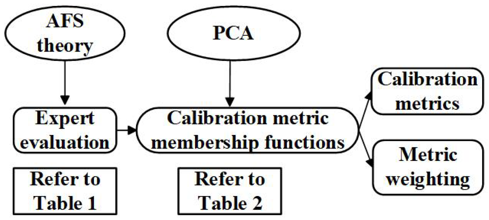
The proposed integrated methodology for the construction of the hydrodynamic model calibration system and the determination of the metric weight, AFS-PCA, follows the workflow shown in Figure 1.

(1) The expert questionnaire design replaced numerical weighting with qualitative tri-level assessments (“critical”, “moderate”, “non-essential”), streamlining response processes while minimizing subjective bias.

(2) Fuzzy quantification: The axiomatic fuzzy set theory converted linguistic assessments into numerical values through mathematical transformation, deriving objective metrics solely from expert inputs.

(3) Metric selection: Processed data underwent principal component analysis to identify key parameters, with component significance determined by eigenvalue magnitudes.

(4) Weight allocation: Normalized eigenvalues quantitatively defined parameter weights through variance proportion calculations.

4. Metric System Architecture Design and Weight Determination Methodology

During metric system design, comprehensive problem analysis typically generates numerous relevant metrics (or factors), each partially characterizing the target objectives through varying information contributions. Expert-informed principal component analysis subsequently eliminates non-contributory indicators exhibiting low calibration efficacy, poor discriminative power, or redundancy. Eigenvectors derived from PCA are then utilized to determine objective metric weights within the optimized system.

4.1. Construction of Model Calibration Metrics and Score Matrix

Formulation of calibration metrics and scoring matrix was guided by practical hydrodynamic model calibration requirements. A preliminary metric set was established through systematic literature review, comparative/analytical/synthetic approaches, and structured expert interviews. A specialized questionnaire was subsequently developed and distributed to a panel of domain experts for metric prioritization using tri-level scoring: “critical”, “moderate” and “non-essential”. With n experts evaluating m metrics, the compiled responses form scoring matrix $X={\left[x_{ij}\right]}_{n\times m}$, where $x_{ij}\in \{3,2,1\}$ corresponds to the three-tier prioritization scale.

$$X=\left[\begin{array}{cccc}{x}_{11}& x_{12}& \cdots & x_{1m}\\ x_{21}& x_{22}& \cdots & x_{2m}\\ \cdots & \cdots & \cdots & \cdots \\ x_{n1}& x_{n2}& \cdots & x_{nm}\end{array}\right]$$

(1)

4.2. Membership Matrix Construction

The transformation from experts’ qualitative assessments to membership degrees is achieved through the AFS axiomatic framework (see [29] for theoretical foundations). The quantification mechanism is formalized as

$${\mu }_{ij}={\displaystyle \frac{\left|\left\{x_{kj}\mid x_{kj}<x_{ij},k=1,2,\cdots ,n\right\}\right|}{n}}$$

(2)

Here, $x_{ki}<x_{ij}$ indicates that the fuzzy evaluation given by the i-th expert for the j-th indicator is higher than or equal to that given by the k-th expert. ${\mu }_{ij}$ represents the membership degree value of the fuzzy evaluation given by the i-th expert for the j-th indicator.

$$\Xi =\left[\begin{array}{cccc}{\mu }_{11}& {\mu }_{12}& \cdots & {\mu }_{1m}\\ {\mu }_{21}& {\mu }_{22}& \cdots & {\mu }_{2m}\\ \cdots & \cdots & \cdots & \cdots \\ {\mu }_{n1}& {\mu }_{n2}& \cdots & {\mu }_{nm}\end{array}\right]$$

(3)

4.3. Calibration Metric System Architecture

We identified which of the aforementioned m metrics could be used to construct the calibration metric system through PCA. The goal is to make modifications to traditional PCA. Traditional PCA aims to eliminate metrics with insignificant variations across all samples, but this contradicts the aforementioned practical requirements for metric selection. In metric evaluation, low variation in expert opinions on a specific metric indicates consensus among experts. Therefore, we retain these metrics characterized by expert consensus and high fuzzy membership degrees. These metrics are then employed to establish the evaluation criteria for hydrodynamic models. The improved PCA methodology is as follows:

(1) Compute the membership matrix:

$$C={\displaystyle \frac{S^{T}S}{n-1}}$$

(4)

where S is the matrix obtained by centering the membership matrix $\Xi$.

(2) Eigenvector Selection: Perform eigenvalue decomposition on the covariance matrix to obtain m eigenvalues: ${\lambda }_1,{\lambda }_2,\dots ,{\lambda }_{\mathrm{m}}$. Select the eigenvector $\alpha ={({\alpha }_1,{\alpha }_2,\dots ,{\alpha }_{\mathrm{m}})}^T$ corresponding to the smallest eigenvalue.

(3) Calibration Metric Feature Analysis: Each component of the eigenvector corresponds to a metric. Select $p_1$ components by sorting their values in ascending order, then retain the corresponding $p_1$ metrics as candidates. Unselected metrics exhibit high “energy” (large divergence in expert evaluations), indicating low consensus among experts, and are therefore discarded.

(4) Calibration Metric System Construction: From the $p_1$ candidate metrics, remove $p_2$ metrics by sorting their mean membership degrees in ascending order. Use the remaining K metrics to establish the metric system (where $K=p_1-p_2$). The rationale for removing metrics with lower mean membership degrees is to prioritize metrics with higher expert evaluation consensus for assessing higher-level metrics.

4.4. Determination of Metric Weights

The normalized results constitute the weights of the K metrics in the established system. ${\omega }_i$ represents the weight of the i-th indicator in the system, i = 1, 2, …… K.

$${\omega }_i={\displaystyle \frac{\frac{1}{|{\alpha }_i|}}{{\sum }_{j=1}^K\frac{1}{|{\alpha }_j|}}}$$

(5)

5. Case Study

This study selects 18 experts to conduct fuzzy evaluations on six metrics obtained through the segmentation of calibration content and methodologies for marine hydrodynamic models, as detailed in

Table 1. Fuzzy evaluation matrix of calibration metrics from expert assessments.

Metric	${\mathit{f}}_1$	${\mathit{f}}_2$	${\mathit{f}}_3$	${\mathit{f}}_4$	${\mathit{f}}_5$	${\mathit{f}}_6$
$e_1$	moderate	critical	critical	critical	critical	critical
$e_2$	critical	critical	critical	critical	moderate	critical
$e_3$	critical	critical	critical	critical	moderate	critical
$e_4$	critical	critical	moderate	moderate	moderate	critical
$e_5$	critical	critical	critical	moderate	moderate	critical
$e_6$	moderate	critical	non-essential	non-essential	non-essential	non-essential
$e_7$	critical	critical	critical	moderate	moderate	critical
$e_8$	critical	critical	critical	moderate	moderate	critical
$e_9$	critical	critical	critical	critical	moderate	critical
$e_{10}$	critical	critical	moderate	moderate	moderate	moderate
$e_{11}$	critical	critical	critical	moderate	moderate	critical
$e_{12}$	critical	critical	critical	critical	critical	critical
$e_{13}$	moderate	critical	moderate	moderate	moderate	moderate
$e_{14}$	critical	critical	critical	critical	critical	critical
$e_{15}$	critical	critical	moderate	critical	critical	critical
$e_{16}$	critical	critical	moderate	critical	critical	critical
$e_{17}$	critical	critical	critical	critical	moderate	critical
$e_{18}$	critical	critical	moderate	moderate	moderate	moderate

Notes: $f_1$: roughness coefficient; $f_2$: bathymetry (water depth); $f_3$: shoreline configuration; $f_4$: open-boundary forcing conditions; $f_5$: thermal–saline parameters; $f_6$: wind field characteristics.

(empirical dataset from Xiamen University and China Institute for Radiation Protection). In Table 1 and

Table 2. Membership values of fuzzy evaluation of calibration indicators by experts.

Metric	${\mathit{f}}_1$	${\mathit{f}}_2$	${\mathit{f}}_3$	${\mathit{f}}_4$	${\mathit{f}}_5$	${\mathit{f}}_6$
$e_1$	0.167	1.000	1.000	1.000	1.000	1.000
$e_2$	1.000	1.000	1.000	1.000	0.722	1.000
$e_3$	1.000	1.000	1.000	1.000	0.722	1.000
$e_4$	1.000	1.000	0.389	0.500	0.722	1.000
$e_5$	1.000	1.000	1.000	0.500	0.722	1.000
$e_6$	0.167	1.000	0.056	0.056	0.056	0.056
$e_7$	1.000	1.000	1.000	0.500	0.722	1.000
$e_8$	1.000	1.000	1.000	0.500	0.722	1.000
$e_9$	1.000	1.000	1.000	1.000	0.722	1.000
$e_{10}$	1.000	1.000	0.389	0.500	0.722	0.222
$e_{11}$	1.000	1.000	1.000	0.500	0.722	1.000
$e_{12}$	1.000	1.000	1.000	1.000	1.000	1.000
$e_{13}$	0.167	1.000	0.389	0.500	0.722	0.222
$e_{14}$	1.000	1.000	1.000	1.000	1.000	1.000
$e_{15}$	1.000	1.000	0.389	1.000	1.000	1.000
$e_{16}$	1.000	1.000	0.389	1.000	1.000	1.000
$e_{17}$	1.000	1.000	1.000	1.000	0.722	1.000
$e_{18}$	1.000	1.000	0.389	0.500	0.722	0.222
mean value	0.861	1.000	0.744	0.725	0.762	0.818

, $e_i$ represents the i-th expert (i = 1, 2, …, 18), and $f_j$ denotes the j-th metric (j = 1, 2, …, 6).

The AFS theory was systematically applied to transform the fuzzy evaluations documented in Table 1 into formal membership degree quantifications. Through rigorous computation via Equation (2), the fuzzy membership degrees corresponding to six calibration metrics assessed by 18 domain experts were obtained, with complete numerical results presented in Table 2.

5.1. Determination of Calibration Indicators

The modified PCA method was applied to analyze the data presented in Table 2.

(1) Covariance Matrix Construction

Covariance matrix C characterizing the membership degree distributions was rigorously derived through Equation (4):

$$C=\left[\begin{array}{cccccc}0.102& 0.000& 0.039& 0.030& 0.025& 0.058\\ 0.000& 0.000& 0.000& 0.000& 0.000& 0.000\\ 0.039& 0.000& 0.115& 0.050& 0.028& 0.087\\ 0.030& 0.000& 0.050& 0.090& 0.049& 0.068\\ 0.025& 0.000& 0.028& 0.049& 0.047& 0.045\\ 0.058& 0.000& 0.087& 0.068& 0.045& 0.124\end{array}\right]$$

(2) Eigenvalue Decomposition of Covariance Matrix C

Covariance matrix C was decomposed to obtain six eigenvalues: ${\lambda }_1$ = 0.000, ${\lambda }_2$ = 0.014, ${\lambda }_3$ = 0.025, ${\lambda }_4$ = 0.062, ${\lambda }_5$ = 0.074 and ${\lambda }_6$ = 0.303. Following PCA convention, components corresponding to zero eigenvalues were discarded. The eigenvector associated with ${\lambda }_2$ = 0.014 was selected: ${(-0.057,0.000,0.125,-0.521,0.838,-0.090)}^{\mathit{T}}$.

(3) Candidate Metric Selection

The first five components ($p_1$ = 5) with the smallest magnitudes were selected: −0.057, 0.000, 0.125, −0.521 and −0.090. These correspond to metrics $f_1$, $f_2$, $f_3$, $f_4$ and $f_6$.

(4) Table Referencing

By consulting Table 2, the mean membership degrees of the five candidate metrics were compared: mean($f_1$) = 0.861, mean($f_2$) = 1.000, mean($f_3$) = 0.744, mean($f_4$) = 0.725 and mean($f_6$) = 0.818. Metric $f_4$ was removed from the candidate set due to its minimum mean value ($p_2$ = 1). The final metric system comprises $f_1$, $f_2$, $f_3$ and $f_6$, with K = $p_1$−$p_2$ = 5 − 1 = 4. As shown in Table 1, metric $f_5$ received low fuzzy evaluations: 12 experts assigned a “moderate” rating, with significant inconsistencies in expert opinions (low consensus). The PCA methodology excluded $f_5$ during initial selection, demonstrating its scientific validity and applicability to such problems.

5.2. Calibration Metric Weight Determination

The weights of $f_1$, $f_2$, $f_3$ and $f_6$ were determined through rigorous computation via Equation (5). The complete calculation process is systematically documented in

Table 3. Weights of $f_1$, $f_2$, $f_3$ and $f_6$.

	${\mathit{f}}_1$	${\mathit{f}}_2$	${\mathit{f}}_3$	${\mathit{f}}_6$
Eigencomponent	$-0.057$	$0.000$	$0.125$	$-0.090$
Norm	$0.057$	$0.000$	$0.125$	$0.090$
Reciprocal	$17.544$	$\infty$	$8.000$	$11.111$
Weight	$0.479$	N/A	$0.218$	$0.303$

.

Analysis of the fuzzy evaluations by experts for each metric in Table 3 reveals that metric $f_2$ received unanimous recognition from all 18 experts, while only 3 experts expressed divergent opinions regarding $f_1$. This observation suggests that $f_1$ should carry greater weight within the system. Moreover, computational results demonstrate a unanimous expert consensus on the critical importance of $f_1$, with its calculated weight of 0.479 aligning fully with prior analytical expectations. These findings confirm the scientific validity of the weighting methodology and its consistency with expert evaluations.

5.3. Calibration Metric Sensitivity Analysis

A parameter sensitivity analysis was conducted on the critical metric $f_1$. The Beibu Gulf was selected as the study area, and a hydrodynamic model was established using the Finite Volume Community Ocean Model to investigate variations in the model’s responses to calibration metrics.

5.3.1. Ocean Numerical Modeling FVCOM

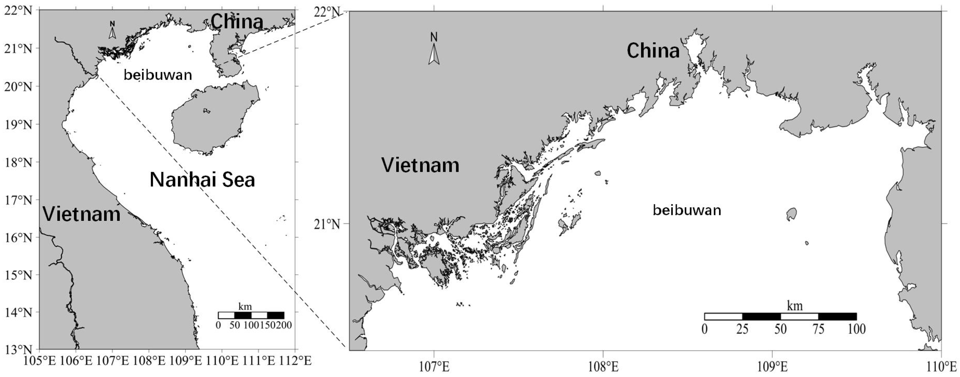
Numerical simulations were conducted using an unstructured mesh spanning 106.5° E–110° E longitude and 20.4° N–22° N latitude. The computational domain consisted of 22,543 grid cells, 12,185 nodes and 53 open-boundary nodes. A four-layer $\sigma$ coordinate system was vertically configured. The model incorporated wet–dry grid detection, cold-start initialization, Smagorinsky parametrization for horizontal eddy viscosity and the Mellor–Yamada 2.5-order turbulence closure model for vertical eddy viscosity.

For the wet–dry grid methodology, water depth was defined as the minimum value relative to mean sea level. Bathymetric data were derived from field measurements by the China Institute for Radiation Protection, with interpolation performed across triangular mesh elements. The simulation area is illustrated in Figure 2, while the corresponding bathymetric distribution and mesh discretization are shown in Figure 3.

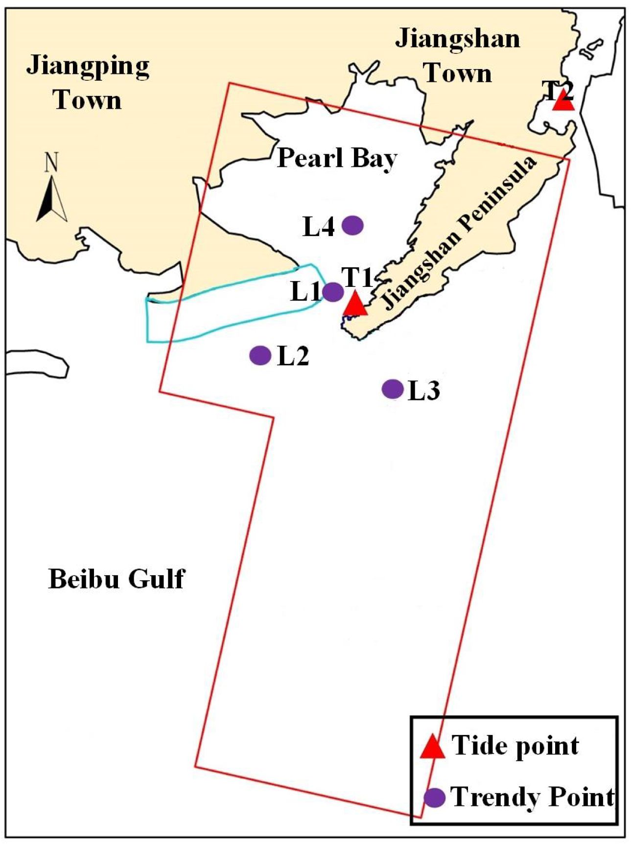
The study simulated hydrodynamic characteristics in the Beibu Gulf from 00:00 on 1 January 2018 to 00:00 on 15 January 2018, with validation performed using field-measured tidal level and current data. The verification datasets were acquired from January 2018 field measurements conducted by the China Institute for Radiation Protection. Based on the hydrodynamic model domain and hydrometric monitoring locations, the monitoring network comprised two tidal gauge stations (Zhenzhu Bay Station [T1] and Fangchenggang Station [T2]) and four current measurement stations (L1–L4), as detailed in Figure 4.

5.3.2. Experimental Condition Setup

The hydrodynamic model was developed using field-measured bathymetric data from the China Institute for Radiation Protection, with adjustments made to the bed roughness coefficient. A comparative analysis was conducted to evaluate tidal level and current variations under different roughness coefficients.

On the basis of FVCOM drag coefficient $C_d$ [40], a control variable d is introduced as shown in the formula

$$F=d·C_d=d·max\left(k^2/ln{({\displaystyle \frac{Z_{ab}}{Z_o}})}^2,0.0025\right)$$

(6)

where k = 0.4 is the von Karman constant, $Z_{ab}$ is the height above the bottom, $Z_o$ is the bottom roughness parameter, and F is the improved roughness coefficient.

To evaluate the sensitivity of metric f₁, this study configured distinct operational scenarios and computed hydrodynamic tidal levels and current dynamics for each case. The experimental case combinations are tabulated in

Table 4. Experimental case configuration.

Metric	Case	Parameters	Compared
F	1	0.5	Tidal levels, Currents
	2	1	Tidal levels, Currents
	3	1.5	Tidal levels, Currents
	4	2	Tidal levels, Currents
	5	2.5	Tidal levels, Currents
	6	3	Tidal levels, Currents
	7	4	Tidal levels, Currents

. Case 2 adopts baseline roughness coefficient settings.

5.3.3. Correlation Analysis Between Simulated and Measured Tidal Levels

Utilizing real-time meteorological data from 00:00 on 1 January to 00:00 on 15 January 2018, this study computed full tidal cycle variations within the model domain. Calculated tidal levels at monitoring stations under all operational cases were systematically compared against field-measured data. The variation patterns of simulated and observed tidal levels are graphically presented in Figure 5.

As shown in Figure 5, during Case 1, simulated tidal currents at Stations T1 and T2 exhibited strong correlation with measured data under spring and mid-tide conditions, demonstrating close agreement between simulated and observed curves, with only minor deviations at the simulation onset. In contrast, neap tide conditions showed significantly reduced correlation between simulated tidal levels and field measurements, along with marked discrepancies in curve morphology. This suggests that roughness coefficients exert greater influence on tidal level accuracy during neap tides compared to spring and mid-tide periods.

To further assess the similarity between measured data and simulation results, this study employed the Pearson correlation coefficient r for quantitative analysis.

$$r(X,Y)={\displaystyle \frac{Cov(X,Y)}{\sqrt{Var\left[X\right]Var\left[Y\right]}}}$$

(7)

In the formula, Y represents the simulated values, where $Cov[X,Y]$ denotes the covariance between X and Y, $Var\left[X\right]$ signifies the variance of X, and $Var\left[Y\right]$ indicates the variance of Y. ${\mathrm{R}}^2$ (coefficient of determination) is mathematically equivalent to the squared Pearson correlation coefficient r.

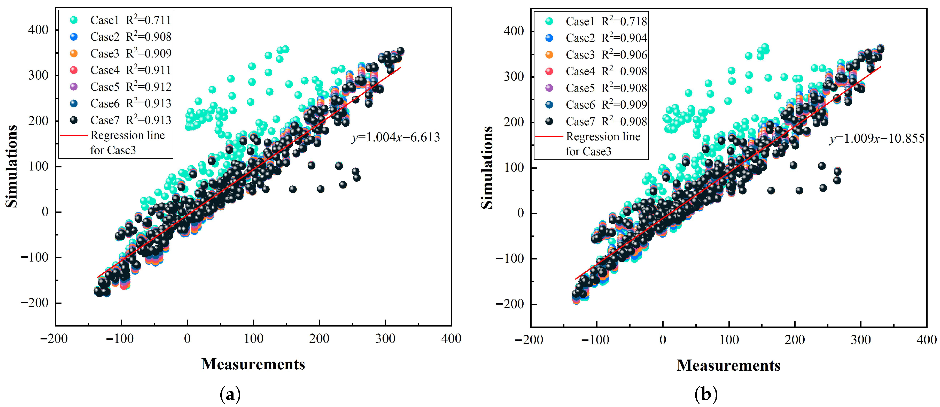
This study computed the Pearson correlation-derived coefficients of determination (R²) between simulated tidal levels and tidal level measurements at monitoring stations under different operational cases, with the results visualized through scatter plot diagrams shown in Figure 6.

As shown in Figure 6, the coefficients of determination (${\mathrm{R}}^2$) for Case 1 at Stations T1 and T2 are below 0.8, while ${\mathrm{R}}^2$ values for Cases 2–7 all exceed 0.9. This demonstrates that Cases 2–7 achieve superior simulation accuracy in reproducing observed tidal fluctuations, with enhanced congruence to measurement data.

5.3.4. Tidal Current Simulation and Measurement Correlation Analysis

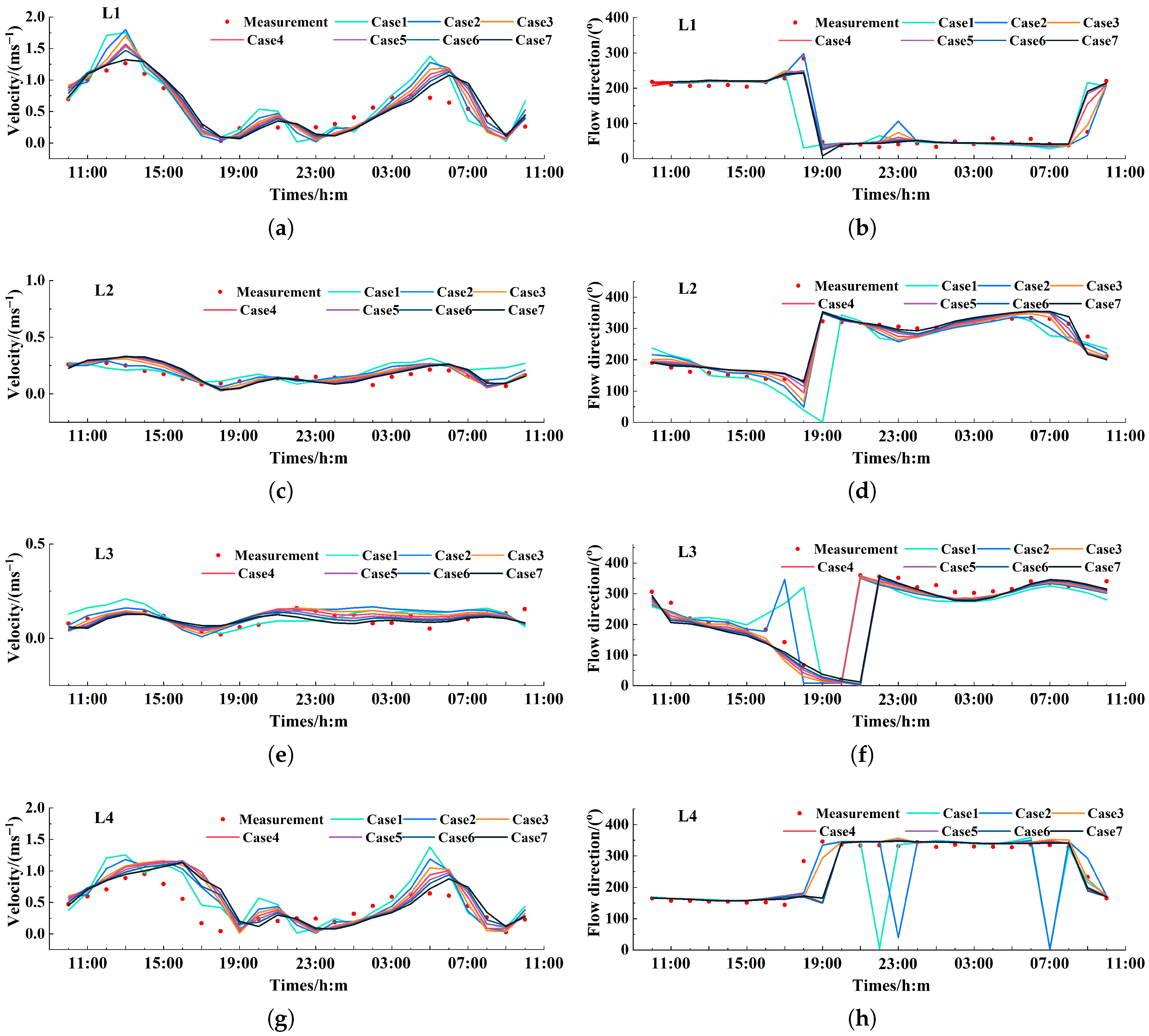
This study computed full tidal-cycle current variations across the model domain and conducted systematic comparisons between simulated tidal currents and field measurements at monitoring stations under various operational cases. Detailed validation outcomes are presented in Figure 7.

As shown in Figure 7, significant differences exist between simulated and measured current directions at tidal stations under Case 1, specifically illustrated in subplots (b), (d), (f) and (h). For all other operational cases, both simulated current velocities and directions agree well with measurement data.

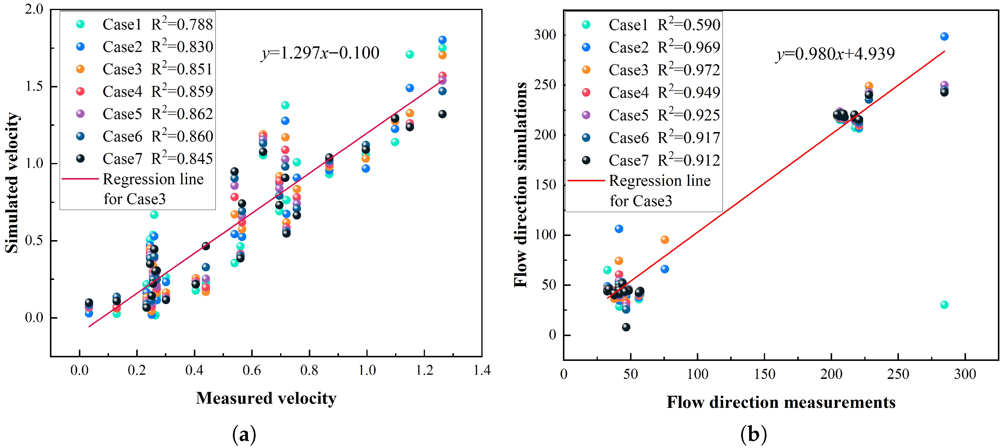
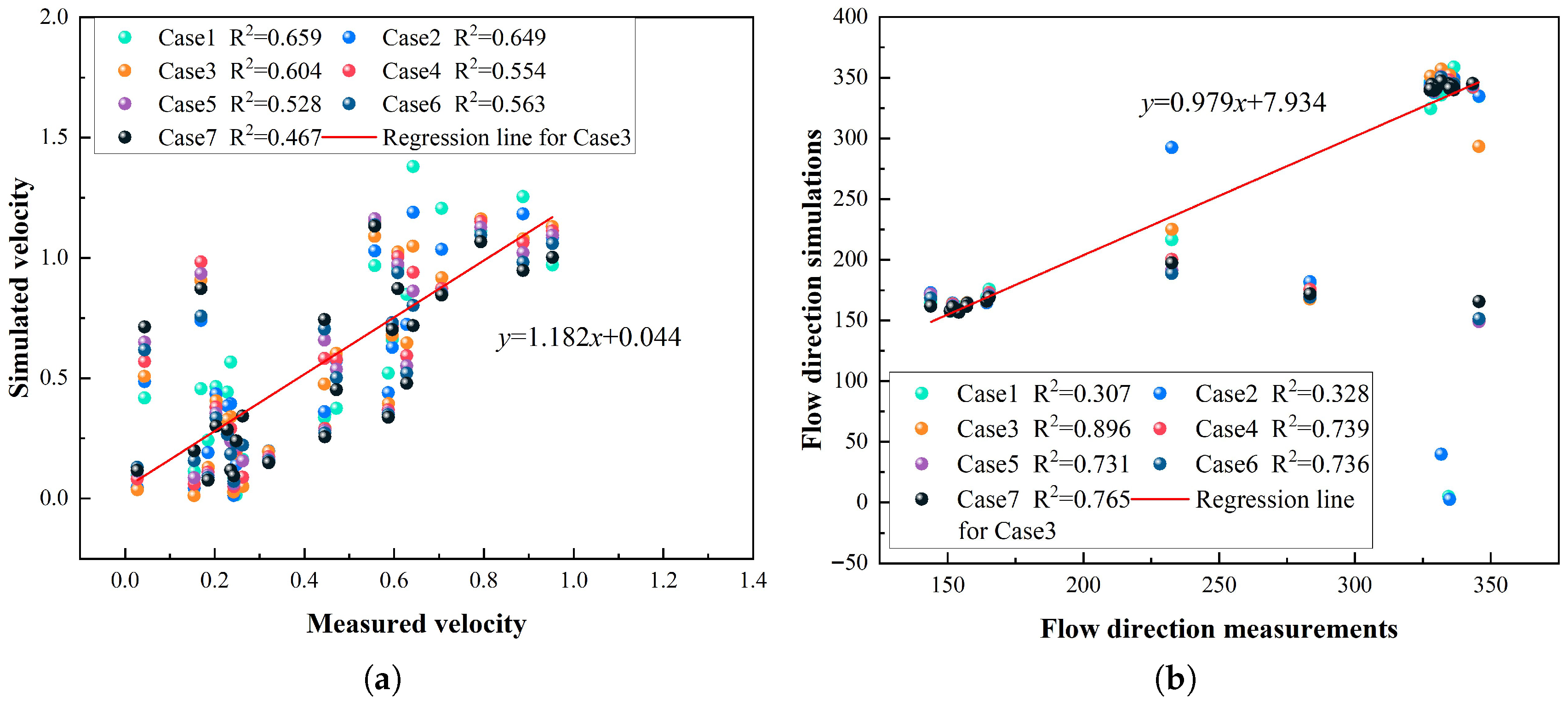
To systematically evaluate the simulation accuracy of tidal currents across operational cases, this study calculated Pearson-derived coefficients of determination (R²) between modeled and measured current velocities/directions at monitoring stations. Comparative scatter plots are provided in Figure 8, Figure 9, Figure 10 and Figure 11.

As shown in Figure 8, Case 1 exhibits lower coefficients of determination (R²) compared to other operational cases, while Cases 2–7 demonstrate relatively higher values, with velocity R² exceeding 0.4 and directional R² surpassing 0.8. Detailed analysis of Figure 8, Figure 9, Figure 10 and Figure 11 reveals that Case 3 achieves the highest R² values (0.851 for velocity, 0.976 for direction), Specifically, the R² for the flow direction of Station L3 in Case 3 is 0.568 higher than that in Case 2, indicating optimal tidal current model agreement between simulated and measured data.

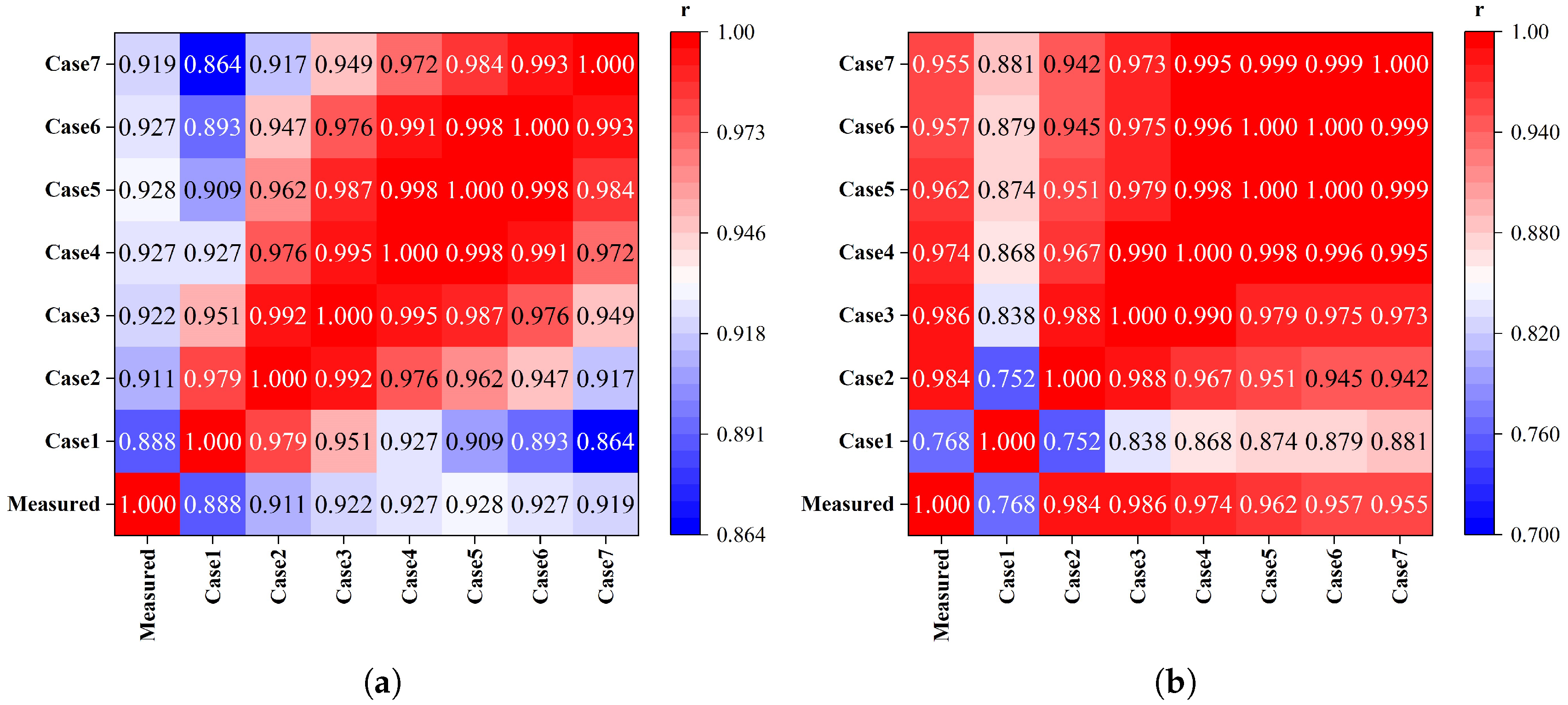
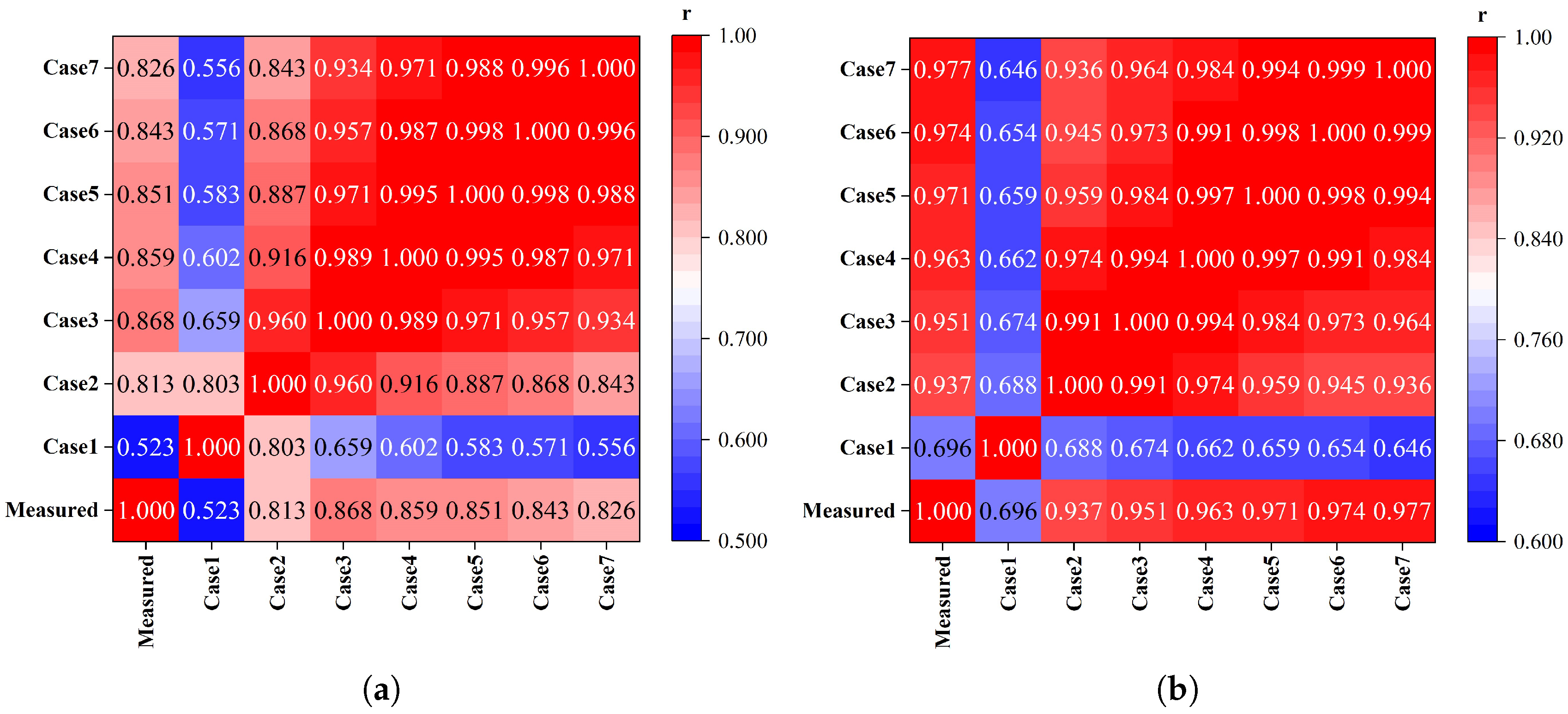
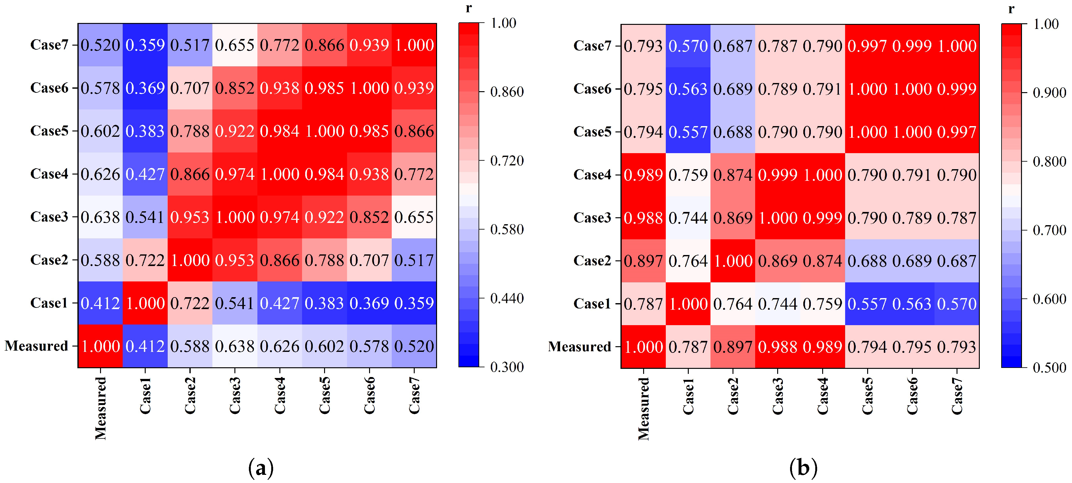
To rigorously evaluate inter-case correlations, this investigation generated heatmaps of tidal current correlation coefficients across operational scenarios at monitoring stations, as visualized in Figure 12, Figure 13, Figure 14 and Figure 15.

The correlation coefficient heatmaps (Figure 12, Figure 13, Figure 14 and Figure 15) reveal consistently positive correlations across Cases 1–7, with no negative correlations observed. Pearson correlation coefficients between Case 1 and Cases 2–7 remain relatively low, in the range of [0.359, 0.953], predominantly indicating weak positive correlations. Higher correlations emerge between Case 2 and Cases 3–7, with coefficients spanning [0.517, 0.992] and mostly reflecting moderate positive relationships. The strongest correlations occur between Case 3 and Cases 4–7, yielding coefficients in the [0.655, 0.992] range where nearly all values exceed 0.9, demonstrating robust positive correlations.

Notably, Cases 3–7 exhibit the highest mutual Pearson correlations, suggesting minimal divergence in their simulation outputs. However, analysis of tidal current scatter plots across cases demonstrates a counterintuitive decline in simulation accuracy from Case 4 to Case 7 as roughness coefficients increase. This degradation is exemplified at Station L3 (Figure 14a), where further roughness amplification causes marked deterioration in current velocity simulation fidelity.

The analysis conclusively demonstrates distinct roughness-dependent correlation regimes: When roughness coefficients range between 1 and 2 times the baseline value, a strong positive correlation exists between simulated and measured tidal levels/currents, confirming effective model-data matching. Beyond 2 × baseline roughness, however, progressive correlation decay occurs with increasing coefficients, directly reflecting intensifying discrepancies between simulated and observed tidal currents.

6. Conclusions

To address the challenges of inconsistent numerical model calibration methods and over-reliance on expert knowledge in hydrodynamic model calibration systems, this study proposes a method combining AFS theory and PCA. Expert questionnaires were conducted to establish a hydrodynamic model for the Beibu Gulf in the South China Sea, calculate calibration indices and their weights, and analyze relationships between simulated and measured data across different cases. Key conclusions are as follows:

(1) A method for determining hydrodynamic model calibration indices and weights based on AFS-PCA integration is proposed. This approach mitigates issues such as subjective biases, insufficient quantitative data and excessive reliance on expert knowledge, enhancing objectivity and accuracy.

(2) The method was applied to identify key calibration indices ($f_1$, $f_2$, $f_3$ and $f_6$, with $f_1$ and $f_2$ being the most critical). The results align closely with expert evaluations, validating the method’s effectiveness.

(3) Comparative analysis of tidal level and current simulation results against field measurements under varying roughness coefficients reveals two distinct operational regimes. For elevated roughness conditions (1–2 times baseline coefficient), strong positive correlations between simulated and measured parameters confirm effective model-data matching. Beyond 2 × baseline roughness, however, progressive correlation degradation accompanies increasing coefficients, demonstrating amplified discrepancies between simulated and observed currents. Conversely, under reduced roughness conditions, high correlation persists during spring and mid-tide periods, whereas neap tide simulations exhibit significantly diminished accuracy, indicating enhanced roughness sensitivity during low tidal energy phases.