Abstract
Glacial-origin lakes in southern South America are increasingly exposed to anthropogenic pressures, but early signs of contamination often remain undetected in apparently pristine systems. In this study, we assessed the bioaccumulation of trace metals (Cu, Mn, Zn, Cr) in the tissues of the native freshwater mussel Diplodon chilensis and their relationship with sediment metal concentrations across 15 sites in six temperate lakes. Sediment quality was largely classified as unpolluted according to the geoaccumulation index (87% of values ≤ 0), yet high metal loads were found in mussel tissues, with Mn and Zn reaching 3325 mg·kg−1 and 350 mg·kg−1 respectively. Bioaccumulation factors were especially high for Mn (42.2) and Zn (32.1), reflecting efficient uptake from the environment. Multivariate analyses revealed spatial patterns driven by sediment composition and gradients of human influence, while regression models highlighted a significant role of fine sediment fractions in Mn bioaccumulation. These results demonstrate that D. chilensis can detect bioavailable metal fractions even in low-impact systems, underscoring its potential as a sentinel species. The integrative approach combining sediment chemistry, tissue analyses, and quantitative indices provides a replicable, cost-effective framework for the early detection of metal contamination in temperate lakes worldwide.
1. Introduction
Glacial-origin lakes are among the most valuable and sensitive freshwater ecosystems worldwide, functioning as critical reservoirs of biodiversity and essential ecosystem services such as water regulation, nutrient cycling, and support for unique aquatic communities [1]. These systems are typically characterized by oligotrophic conditions, high transparency, and low human disturbance, making them ideal reference environments for ecological monitoring and conservation planning [2]. However, emerging pressures such as urban expansion [3], tourism [4], intensive agriculture [5] and aquaculture [6] are increasingly compromising their ecological integrity. These activities often exert subtle but significant impacts that may go undetected using conventional monitoring methods.
Among these stressors, trace metals represent a particularly persistent and complex threat due to their tendency to accumulate in sediments and become bioavailable under changing physicochemical conditions [7]. While total metal concentrations in sediments are commonly used as indicators of contamination, they do not necessarily reflect the bioavailable fraction that can be taken up by aquatic organisms [8]. This is because metal mobility and toxicity are influenced by factors such as particle size, organic matter content, pH, and redox conditions. As a result, more integrative approaches, such as sequential extraction methods or in situ techniques, have been recommended to estimate bioavailable fractions under realistic field conditions [9].
In this context, the use of benthic bioindicators, especially filter-feeding bivalves, has proven effective for assessing biological exposure to metals and other persistent contaminants in aquatic ecosystems [10]. Among these organisms, Diplodon chilensis Gray, 1828 (Hyriidae), a freshwater bivalve endemic to southern South America, stands out for its wide distribution, longevity, and filtering behavior, which enable it to integrate environmental conditions over time [11,12,13]. This species is also the dominant benthic component in many temperate lakes of Chile and Argentina, due to its high abundance, biomass, and lifespan [14], as well as its functional role in filtering large volumes of water [15]. Its structural presence influences sediment stabilization, nutrient cycling, and water quality, reinforcing its value as an ecological sentinel. Despite these attributes, its use in environmental monitoring programs has been limited, especially in lakes with low human impact, which restricts the establishment of baseline conditions for detecting subtle disturbances.
This study was conducted in six temperate lakes of southern South America that span a natural gradient of human influence, ranging from catchments dominated by native forest to those affected by urban and aquaculture activities [16]. Although these lakes differ in morphology and land use, they all exhibit high environmental quality and are representative of glacial lake ecosystems [17].
We hypothesized that even in low-impact systems, early signs of metal contamination can be detected through an integrated approach combining sediment analysis and metal bioaccumulation in D. chilensis. The specific objectives were (1) to characterize sediment texture and organic matter content at sites with different levels of human activity, (2) to quantify Cu, Mn, Zn, and Cr concentrations in surface sediments and bivalve soft tissues during winter and summer, (3) to assess metal bioavailability using the geoaccumulation index (Igeo), the bioaccumulation factor (BAF), and the metal pollution index (MPI), and (4) to analyze spatial patterns and differences between sampling periods using multivariate statistics and regression models. The selection of Cu, Mn, Zn, and Cr was based on previous studies conducted in Lake Nahuel Huapi, a nearby and ecologically comparable system, where these metals were shown to be sensitive indicators of environmental variability. In contrast, other elements offered limited interpretive value [12,18].
This integrated approach enables the assessment of trace metals not only in abiotic and biological compartments but also in terms of their bioavailability under local ecological conditions. By focusing on systems with minimal human disturbance, this study provides valuable reference data for early detection of environmental change in temperate glacial lake ecosystems of southern South America.
2. Materials and Methods
The study was conducted in six temperate lakes located in the North Patagonian Lake District of Chile: Neltume, Colico, Panguipulli, Rupanco, Llanquihue, and Villarrica. These lakes were selected to represent a gradient of anthropogenic influence, ranging from highly natural conditions to systems subjected to urban and aquaculture pressures (Table 1, Figure 1). Characterization was based on limnological criteria, native forest cover, human settlements, and aquaculture concessions, according to data reported [14,16,19]. All lakes are of glacial origin, exhibit oligotrophic to mesotrophic conditions, and have high transparency, making them suitable reference systems for detecting subtle alterations in environmental quality [17].

Table 1.
Morphometric, limnological and anthropogenic attributes of the studied lakes, ordered by degree of human intervention (very low, low, moderate). For each lake/site, we report geographic coordinates (WGS84; decimal degrees), trophic status [20], Secchi depth (m), elevation (m a.s.l.), maximum depth (m), lake surface area (km2), watershed area (km2), native forest cover (%), and the number of settlements with >100 inhabitants (population in parentheses) within the watershed. Site codes match those used throughout the manuscript. Data compiled from [14,19,21,22,23,24].
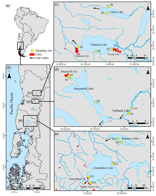
Figure 1.
Location of the 15 sampling sites (S1–S15) across six lakes in the North Patagonian Lake District, southern Chile. (a) Overview map of South America indicating the study region; (b) regional map of the study area; (c) Villarrica (S1–S3) and Colico (S4–S5); (d) Panguipulli (S6–S7) and Neltume (S8–S10); (e) Llanquihue (S11–S13) and Rupanco (S14–S15). Yellow circles denote sampling sites; arrows indicate lake outlet rivers. Nearby cities are shown for geographic reference. Coordinate reference system: WGS84 (geographic latitude/longitude). Site coordinates are provided in Supplementary Material Table S1.
Sampling was conducted at 15 sites distributed across the six studied lakes (Figure 1). The geographic coordinates (UTM, WGS84) of each site are provided in Supplementary Material Table S1. Within each lake, sites were selected to represent spatial variability in potential exposure to anthropogenic influences and to capture contrasting limnological conditions. Sampling was performed during two contrasting seasonal periods, winter (2018) and summer (2019), to examine the temporal stability of spatial patterns in metal bioavailability and bioaccumulation among lakes.
During the winter (July 2018) and summer (February 2019) campaigns, in situ physicochemical parameters were measured at each sampling site from the surface to 5 m depth using a pre-calibrated multiparameter probe (Hanna HI 9828, Hanna Instruments, Woonsocket, RI, USA). The variables recorded included temperature (°C), pH, electrical conductivity (µS/cm), and dissolved oxygen (mg/L). These measurements were used to characterize the physicochemical environment of the bottom water and to support the interpretation of spatial and temporal patterns in metal bioavailability and bioaccumulation across lakes.
Sampling of sediments and Diplodon chilensis tissues was conducted at 5 ± 1 m depth, where this species reaches its highest densities in temperate lakes (50–500 ind/m2 [14]). At each site, 20 × 20 m quadrants were defined using random coordinates (X, Y). Surface-sediment samples (0–10 cm) were collected in triplicate (n = 3 sediment replicates) with a 5 cm diameter PVC corer for granulometric and organic matter (OM) analyses. Simultaneously, five adult specimens of D. chilensis (shell length 40–72 mm, 61 ± 9 mm; n = 5 biological replicates) were hand-collected by scuba diving. All individuals corresponded to adults in reproductive age, which, according to reference [14], represent specimens between 5 and 8 years old based on sclerochronological readings. Organisms were placed in bags with lake water and transported in refrigerated boxes to the laboratory. To eliminate pseudofeces and gut contents, the bivalves were kept in filtered water at 4 °C for 24 h [25,26]. In two sites (S13-winter and S6-summer), no specimens were found, so only sediment data were collected.
Sediment samples were dried at 60 °C for 12 h and subsequently dry-sieved through 1000 µm and 63 µm meshes. This process allowed the differentiation of three fractions: gravel (>1000 µm), sand (63–1000 µm), and mud (<63 µm), the latter comprising silt and clay. The weight of each fraction was determined using an analytical balance (Sartorius ENTRIS2202-1S, Sartorius AG, Göttingen, Germany) to calculate their relative proportions. Organic matter content was then estimated via loss on ignition, incinerating dry subsamples at 500 °C for 3 h [27].
Sediments (<63 µm fraction, dried at 105 °C) were homogenized, ground, and digested with an HF:HNO3 (2:1) mixture at 90 °C in a closed system, following an adapted EPA 3052 protocol [28,29]. Soft tissues were extracted from specimens, lyophilized (Labconco Corporation, Kansas City, MO, USA), ground in an agate mortar, and digested with 20 mL of HNO3 (Suprapur®, Merck KGaA, Darmstadt, Germany) at 90 °C with constant agitation [30,31]. Only the soft tissues (whole body without shell) were used for chemical analyses to ensure standardized comparisons among individuals and sampling sites, following common protocols for freshwater bivalves [30,31]. Solutions were diluted and filtered (Whatman 42) prior to analysis.
Concentrations of Cu, Zn, Mn, and Cr were determined by flame atomic absorption spectrophotometry (Unicam 969, Thermo Scientific, Waltham, MA, USA, and ICE 3000, Thermo Fisher Scientific, Waltham, MA, USA, air–acetylene flame), and for the determination of chromium, a nitrous oxide–acetylene flame was used, following adapted protocols from [28,29]. Sediment samples (<63 µm fraction, dried at 105 °C) were ground, sieved, and digested with an HF:HNO3 (2:1) mixture at 90 °C in a closed system, according to an adapted EPA 3052 method [30]. Tissue samples (1.0 g dry weight) were lyophilized (Labconco Corporation, Kansas City, MO, USA), ground in an agate mortar, and digested with 20 mL of Suprapur HNO3 (Merck, Darmstadt, Germany) at 90 °C under constant agitation until near dryness, then diluted to a final volume of 50 mL with double-distilled water. All reagents were of high-purity analytical grade (Suprapur, Merck, Darmstadt, Germany), and calibration curves were prepared from certified single-element standards (Fisher Scientific, Waltham, MA, USA) with five concentration points (R2 > 0.999).
Instrumental limits of detection (LOD) and quantification (LOQ) were determined as 3× and 10× the standard deviation of blank signals, respectively, following IUPAC guidelines [31]. LODs/LOQs (mg·kg−1) were 0.008/0.026 for Cu and Mn, 0.004/0.014 for Zn, and 0.004/0.013 for Cr.
In soft tissues, Cr concentrations were frequently below the laboratory quantification limit (LOQ = 0.01 mg·kg−1), reflecting trace levels near the detection capability of FAAS for this element. For statistical analyses, values reported as below LOQ were replaced by LOQ/2 to preserve numerical consistency without biasing correlations. Analytical quality was verified through reagent blanks, duplicate samples, and certified reference materials (MESS-1, National Research Council Canada (NRC-CNRC), Ottawa, ON, Canada, for sediments and TORT-1, National Research Council Canada (NRC-CNRC), Ottawa, ON, Canada, for tissues), with recoveries ranging from 87.5% to 104% and relative errors from −12.5% to 4% (Table 2), confirming the reliability and accuracy of the results. Each sample was analyzed in duplicate, including a control solution. All concentrations were expressed as mg·kg−1 dry weight.
Table 2.
Analytical validation using certified reference materials (CRMs) from NRC Canada: MESS-1 (sediment) and TORT-1 (tissues). For each element, certified and measured concentrations are given in mg·kg−1 (dry weight) as mean ± SD (n = 3 independent digestions). Also shown are relative error (%) and recovery (%), calculated as [(observed − certified)/certified] × 100 and (observed/certified) × 100, respectively. In this study, recoveries ranged from 87.5 to 104.0% and relative errors from −12.5 to 4.0%, supporting the accuracy of the analytical procedure.
To assess metal contamination and biological uptake, three complementary indices were applied. The geoaccumulation index (Igeo [32]) was used to evaluate the relative degree of contamination in sediments, with background values defined as the arithmetic mean of metal concentrations across all sites and both sampling periods within each lake [33], thereby avoiding the use of external references that could introduce systematic errors. According to this index, values were classified as Class 0 (Igeo ≤ 0, unpolluted), Class 1 (0 < Igeo ≤ 1, moderately polluted), and Class 2 (1 < Igeo ≤ 2, polluted). In parallel, a bioaccumulation factor (BAF) was calculated for each site and season as the ratio between the concentration of each metal in the soft tissues of D. chilensis and its corresponding concentration in surface sediments, thus providing an estimate of biological uptake efficiency [34]. Finally, the metal pollution index (MPI) was determined for each D. chilensis sample as the geometric mean of Cu, Zn, Mn, and Cr concentrations, as described by [35], thereby summarizing the overall metal burden in tissues and enabling multimetal comparisons across sites.
Pearson correlation coefficients (r) were calculated to evaluate associations between granulometric fractions (mud, sand), OM, and metal concentrations by sampling period and across the entire dataset (n = 30). A Principal Component Analysis (PCA) was conducted using standardized data (Z-score), including granulometric variables, OM, and metals (Cu, Zn, Mn, Cr), following [36]. Based on the PCA coordinates, a K-means clustering was performed, selecting the optimal number of groups using the Silhouette index, and multivariate differences between clusters were tested using MANOVA (Wilks’ Lambda).
Prior to analysis, data were checked for normality and homoscedasticity; variables showing skewed distributions were log10(x + 1)-transformed, and proportions were arcsine-square-root transformed. The significance level was α = 0.05 (two-tailed). To account for potential non-independence of sites nested within lakes, ordinary least squares models were verified using cluster-robust standard errors by lake, yielding consistent results.
Multiple linear models were fitted to assess the effect of total metal concentration in total sediments (Sed), fine fraction (Mud), and OM on metal concentrations in tissues. Models were built using all sites with paired data (n = 28), and effects were considered significant when p < 0.05 [37]. All statistical analyses were conducted in R version 4.3.2 (R Core Team, R Foundation for Statistical Computing, Vienna, Austria) [38].
3. Results
3.1. Physicochemical Characteristics of Bottom Water
Bottom water parameters showed differences between sampling periods, consistent with lake climatic dynamics (Table 3). Temperature ranged from 9.1 °C (Villarrica S1, winter) to 21.1 °C (Colico S4, summer), revealing a typical summer increase of 8 to 10 °C in temperate Southern Hemisphere lakes. The pH remained slightly alkaline (7.35–8.87), with no marked differences among sites or sampling periods.
Table 3.
Physicochemical parameters of bottom water at 7 m depth and surface-sediment characteristics (0–10 cm) at the 15 sampling sites. Seasons: W = winter (July 2018), S = summer (February 2019). Water variables: temperature (°C), pH, conductivity (µS cm−1), and dissolved oxygen (mg L−1). Sediment variables: sand (%), mud (%) = silt + clay < 63 µm, and organic matter (OM, %). Sediment values are reported as mean ± SD (n = 3).
Electrical conductivity varied between 10 µS/cm (Colico S5, summer) and 120 µS/cm (Panguipulli S6, winter). In most sites, values were below 80 µS/cm, within the reference range for oligotrophic systems. However, persistently elevated values (≥100 µS/cm) were recorded at Villarrica S3-summer (100 µS/cm), Panguipulli S6-winter (120 µS/cm), and Llanquihue S12–S13-summer (110 µS/cm), suggesting localized anthropogenic influence. Dissolved oxygen remained high (8.2–12.6 mg/L) across all sites, with no evidence of hypoxia in either sampling period.
3.2. Sediment Granulometry and Organic Matter
Surface sediments (0–10 cm) were generally dominated by the coarse fraction. According to Table 3, mud content ranged from 0.04% (Llanquihue S12, winter) to 6.61% (Neltume S9, summer), reflecting active hydrodynamics and low fine particle deposition. Low standard deviation in most sites indicated high replicate homogeneity and minimal differences between sampling periods, suggesting sedimentary stability.
Three relevant exceptions were identified. In Villarrica, S3 and S1 recorded the highest mud content in winter (43.67% and 30.21%), which dropped to 4.13% and 1.18% in summer, respectively. Winter heterogeneity in S1 may be linked to Cautín River currents, while differences between sampling periods in S3 likely result from southwestern winds promoting summer resuspension. In contrast, Panguipulli S7 showed an increase from 3.04% (winter) to 17.20% (summer), probably due to its sheltered location, which favors summer fine sediment deposition and reduced winter resuspension from northern storms.
Organic matter (OM) content was generally low (0.01–4.73%), with higher values in sites with more mud. Most sites showed OM <1%, typical of well-oxygenated littoral sediments with low sustained deposition.
3.3. Metal Contamination in Surface Sediments
Concentrations of Cu, Mn, Cr, and Zn (mg·kg−1) in surface sediments (0–5 cm) are detailed in Table 4. The overall pattern was Mn > Zn > Cu > Cr. In winter, Villarrica S3 showed the highest Cu concentration (49.58 ± 0.17), while the summer maximum was 19.67 ± 0.41 in Villarrica S1. For Mn, maximum values occurred in Llanquihue S11 (339.42 ± 8.35, summer; 320.87 ± 7.36, winter) and S12 (342.88 ± 15.51, summer). Cr peaked in Llanquihue S11 and S12 during summer (23.90 ± 1.04 and 23.86 ± 1.49). Zn was also highest at Villarrica S3-winter (74.90 ± 1.52).
Table 4.
Metal concentrations and geoaccumulation index (Igeo) in surface sediments (0–5 cm) at the 15 sampling sites. Seasons: W = winter (July 2018); S = summer (February 2019). Sediment concentrations of Cu, Mn, Cr, and Zn are reported in mg·kg−1 (dry weight) as mean ± SD (n = 3). Igeo was computed as Igeo = log2[Cn/(1.5·Bn)] [32], where Cn is the measured concentration and Bn the background value (see Methods for background source). Igeo classes: ≤0 unpolluted; 0–1 unpolluted to moderately polluted; 1–2 moderately polluted; 2–3 moderately to strongly polluted; >3 strongly to extremely polluted.
The geoaccumulation index (Igeo) classified most sediments as unpolluted (Class 0), although some sites fell into the “unpolluted to moderately polluted” category (Class 1). In winter, the highest Igeo values were observed at Villarrica S3 for Cu (1.06) and Zn (0.67). Cr had positive values at Llanquihue S11 (0.17), S12 (0.66), and Rupanco S14 (0.13) and S15 (0.08). In summer, only Llanquihue S11 and S12 showed positive Igeo for Mn (0.27–0.29) and Cr (0.56), still within Class 1.
3.4. Correlations Between Sediment Parameters and Metals
In summer (n = 15), significant correlations were Mud–OM (r = 0.83, p < 0.001), Zn–OM (r = 0.72, p < 0.01), Mud–Zn (r = 0.56, p < 0.05), and Mn–Cr (r = 0.80, p < 0.001).
In winter (n = 15), significant correlations were Mud–Cu (r = 0.73, p < 0.05), Mud–Zn (r = 0.62, p < 0.05), OM–Zn (r = 0.63, p < 0.05), Cu–Zn (r = 0.73, p < 0.001) and Mn–Cr (r = 0.73, p = 0.01). Full correlation matrices with significance marks are shown in Figure 2.
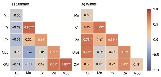
Figure 2.
Heatmap of Pearson correlation matrices for summer (a) and winter (b) samples (n = 15). Significant associations highlight seasonal differences in the coaccumulation of metals and sediment characteristics: Mn–Cr, Zn–OM, and Mud–OM correlations dominate in summer, while Cu, Cr, Zn, and Mud show stronger interrelations in winter (* p < 0.05, ** p < 0.01, *** p < 0.001).
3.5. Multivariate Analysis of Sediments
The Principal Component Analysis (PCA) of combined sediment samples (winter and summer) explained 62.7% of total variability. PCA1 (36.2%) represented the metal load gradient, driven by Zn (31.8%), Cr (20.3%), and Cu (20.2%), while PCA2 (26.5%) was linked to physical properties, mainly mud (24.1%), Mn (23.4%), and sand (19.4%) (Figure 3).
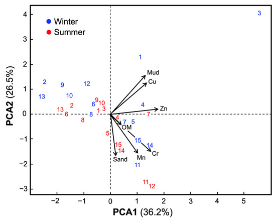
Figure 3.
PCA biplot of surface-sediment attributes and metals for the 15 sampling sites (two seasons; n = 30 observations). Variables included: sand (%), mud (% < 63 µm), organic matter (OM, %), and metal concentrations in surface sediments (mg·kg−1 dry weight: Cu, Mn, Cr, Zn). Points are site scores (winter = blue, summer = red); numeric labels are site codes (1–3 = Villarrica; 4–5 = Colico; 6–8 = Panguipulli; 9–10 = Neltume; 11–13 = Llanquihue; 14–15 = Rupanco). Arrows are variable loadings (direction indicates correlation with the axes; length reflects contribution). The axes show the variance explained (PC1 = 36.2%, PC2 = 26.5%).
Winter sites tended to be associated with fine fractions and higher metal loads, while summer sites grouped in regions dominated by coarse sediments. Villarrica S3-winter had the highest PCA1 score (5.58), reflecting the study’s highest metal load.
K-means clustering based on PCA coordinates identified three clusters (Figure 3; Silhouette score = 0.45). Cluster 1 (gray) grouped most sites with intermediate metal concentrations and high sand content (78.7%). Cluster 3 (green) included sites with the lowest Cu (15.6 mg·kg−1), Zn (30.8), Cr (9.6), and Mn (142.7), along with higher mud (5.1%) and OM (1.36%), representing more natural conditions. Cluster 2 consisted exclusively of Villarrica S3-winter, with the highest Zn (74.9), Cu (49.6), and mud (43.7%).
The overlay of Igeo classes in PCA space (Figure 4) showed that most Cluster 1 and 3 sites were Class 0 (unpolluted), while those with Igeo Class 1 or 2 clustered in Cluster 2 or on Cluster 3 margins. Villarrica S3-winter was the only site classified as Igeo Class 1 for Cu and Class 2 for Zn. MANOVA confirmed significant differences between clusters 1 and 3 (Wilks’ Lambda = 0.501; F = 3.123; p < 0.05), supporting structured groupings based on granulometry and metal load.
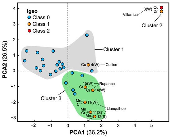
Figure 4.
PCA biplot of surface-sediment variables for the 15 sites in two seasons (n = 30 observations). Variables: sand (%), mud (% < 63 µm), organic matter (OM, %), and metal concentrations in sediments (mg·kg−1 dry weight: Cu, Mn, Cr, Zn). Point fill colors encode Igeo classes computed per site–season: blue = Class 0 (unpolluted), orange = Class 1 (unpolluted to moderately polluted), and red = Class 2 (moderately polluted). Labels indicate lake and site (e.g., “11(W)” = site 11, winter). Shaded polygons are K-means clusters (K = 3) obtained on PCA scores; K was selected by the Silhouette index (0.45). Group differences among clusters were tested with MANOVA (Wilks’ Λ = 0.501; F = 3.123; p = 0.019).
3.6. Metal Content in Soft Tissues
Metal concentrations in D. chilensis soft tissues showed broad spatial variability and differences between sampling periods (Table 5). No samples were collected at S13-winter or S6-summer. The general pattern was Mn > Zn > Cu > Cr. Mn was the dominant metal, ranging from 992.90 mg·kg−1 (Villarrica S1-summer) to 3325.26 mg·kg−1 (Neltume S9-summer). High values were also observed at Llanquihue S13-summer (3114.17) and Rupanco S14-summer (3002.57). Zn peaked at Colico S5-summer (349.57 mg·kg−1), followed by Rupanco S14-summer (296.43), with the lowest values at Villarrica S3-winter (179.04) and Rupanco S15-summer (162.76). Cu ranged from 3.94 mg·kg−1 (Villarrica S2-summer) to 30.00 mg·kg−1 (Villarrica S3-winter), generally higher in winter. High values of Cu were also recorded in Llanquihue S10-winter (22.33). Cr concentrations were generally low or below quantification limits (<0.01 mg·kg−1) at several sites (Panguipulli S7, S8; Neltume S10; Llanquihue S12; Rupanco S14, S15). Maximum values of Cr were at Villarrica S3-winter (11.59 mg·kg−1) and Llanquihue S13-summer (7.98).
Table 5.
Trace metal concentrations (mg·kg−1, dry weight) in soft tissues of Diplodon chilensis, metal pollution index (MPI), and bioaccumulation factors (BAFs) at the sampling sites. No tissue samples were obtained at S13-winter and S6-summer; therefore, no data are reported for these cases. Seasons: W = winter (July 2018), S = summer (February 2019).
3.7. Bioaccumulation Factors (BAFs)
BAFs were calculated only for sites with tissue samples, excluding S13-winter and S6-summer (Table 5). Absolute values were low (BAF < 100) for all metals. Mn showed the highest BAFs, peaking at 42.18 in Neltume S9-summer, followed by Llanquihue S13-summer (30.51), indicating strong bioaccumulation potential.
Zn also showed high BAFs, with a maximum of 32.07 in Llanquihue S13-summer. In contrast, Cu had low and relatively stable BAFs, peaking at 2.10 in Neltume S10-winter. Cr had the lowest BAFs, near zero at most sites, except for specific cases in Villarrica S2-winter (1.55) and Llanquihue S13-summer (1.26). Overall, BAF patterns indicate higher bioaccumulative affinity of D. chilensis for Mn and Zn and lower retention of Cu and Cr, with BAF values for Cu, Zn, and Mn consistently above 1 in most sites, indicating active bioaccumulation, while Cr showed lower but still positive enrichment in soft tissues. Mean BAF values ranged between 1.3 and 3.2 for Cu and Zn.
3.8. Metal Pollution Index in Tissues (MPI)
The Metal Pollution Index, calculated from Cu, Zn, Mn, and Cr concentrations in soft tissues, ranged from 14.59 to 95.87 (Table 5). Sites without tissue data (S13-winter and S6-summer) were excluded. Highest MPI values were observed at Villarrica S3-winter (95.87), Llanquihue S13-summer (94.20), and S12-summer (92.88), coinciding with maximum accumulated Mn and Zn concentrations. The lowest values were at Panguipulli S7 and S8 (14.59 in winter) and Rupanco S15-winter (15.84). These results confirm that MPI effectively summarizes total metal burden in organisms, highlighting sites with the highest bioaccumulation.
3.9. Relationships Between Metal Concentrations in Sediments and Tissues
Global correlation analysis (n = 30) revealed a significant relationship only for Cu (r = 0.42; p < 0.05) between sediments and tissues. No significant correlations were found for Mn, Zn, or Cr. In winter (n = 14), significant correlations were observed for Mn (r = 0.59; p = 0.026) and a marginal trend for Cu (r = 0.51; p = 0.063). In summer (n = 14), no significant associations were found (p > 0.05).
Multiple regression models identified significant effects of sediment variables on bioaccumulation (Table 6). Mud content was positively associated with Mn (coef. = 0.317; p = 0.003) and Cr (coef. = 0.137; p = 0.047). OM showed a negative effect on Mn (coef. = −3.195; p < 0.05) and a marginally positive effect on Zn (coef. = 13.97; p < 0.10). Total metal concentrations in sediments were not significant predictors for any modeled metals.
Table 6.
Multiple regression models were used to explain the bioaccumulation of Zn, Cu, Mn, and Cr in Diplodon chilensis tissues using the total metal concentration in surface sediments (Sed, mg·kg−1 dry weight), the percentage of fine fraction (Mud, % silt + clay, <63 μm), and organic matter content (OM, %) as predictors. The models were fitted using ordinary least squares. Reported values include the coefficient of determination (R2), the p-value of the global model, the F-statistic (degrees of freedom), and the estimated coefficients for each predictor (Coef.). Statistical significance: p < 0.05 (*); ns = not significant.
4. Discussion
This study demonstrates that even temperate glacial lakes considered to be of high environmental quality exhibit incipient signs of trace metal contamination, both geochemically and biologically. The integration of physicochemical parameters, sediment properties, metal concentrations, and bioaccumulation in D. chilensis allowed the detection of subtle accumulations that go unnoticed using conventional indicators [11]. The consistent occurrence of BAF > 1 for most trace metals, together with significant correlations between sediment and tissue concentrations, provides quantitative evidence supporting the interpretation of bioaccumulation in D. chilensis under low-level contamination gradients. Nevertheless, because metal concentrations in both sediments and tissues were low and spatial variability among sites was relatively high, this interpretation should be viewed as indicative rather than conclusive of bioaccumulation under low-level contamination conditions.
The interpretation of metal concentrations in D. chilensis tissues must take into account the fact that this study quantified total metal levels in the <63 µm sediment fraction rather than the truly bioavailable forms. Accordingly, the joint evaluation of fine sediment (<63 µm) and soft-tissue metal concentrations should be regarded as an indirect indicator of metal bioavailability rather than a direct measure. In freshwater unionids, fine particles have been shown to play a dominant role in metal transfer, as sediment-bound species often represent the main exposure route compared to the dissolved phase [39,40]. Moreover, bioaccumulation in these mussels reflects not only environmental availability but also internal physiological regulation through metallothionein synthesis and other homeostatic mechanisms [41]. Together, these findings emphasize that bioaccumulation patterns emerge from the combined influence of sediment geochemistry and species-specific physiological control.
Although temperature, pH, dissolved oxygen, and conductivity remained within reference ranges for oligotrophic systems [14], localized increases in conductivity (≥100 µS/cm) were observed during summer in Villarrica, Panguipulli, and Llanquihue, suggesting period-specific anthropogenic inputs. This pattern aligns with studies documenting the impact of tourism on limnological parameters even in seemingly pristine ecosystems [4,42].
Surface sediments exhibited granulometric heterogeneity, with dominance of coarse fractions and increases in mud in sites such as Villarrica S3-winter (43.67%) and Panguipulli S7-summer (17.20%). This variability was associated with differential retention of organic matter (OM), confirming the functional relationship between granulometry and OM [43]. Metal concentrations were low to moderate (Mn > Zn > Cu > Cr), but maximum values of Cu (49.58 mg·kg−1) and Zn (74.90 mg·kg−1) in Villarrica S3-winter were classified as “moderately contaminated” according to the Igeo index. These results reflect patterns similar to those reported for alpine lakes, where contaminant accumulation occurs despite pristine appearances [42,44,45].
Compared to international benchmarks (Table 7), metal concentrations in southern Chilean lakes fell within low to moderate ranges. Mn values (78.8–342.9 mg·kg−1) were lower than those reported for North Patagonian or urban systems such as Budi Lagoon. Cu (8.48–49.6), Zn (8.45–74.9), and Cr (3.2–23.9) concentrations were also lower than those found in eutrophic or urban systems (e.g., Venice Lagoon, Vembanad Lake), indicating limited contamination.
These comparisons confirm that the studied lakes remain within internationally accepted background or low-contamination levels, consistent with the high environmental quality expected for temperate oligotrophic systems.
The selection of Cu, Zn, Mn, and Cr was based on their ecological relevance and usefulness in previous studies in Lake Nahuel Huapi [12,18], where they exhibited meaningful spatial patterns.
Multivariate analysis confirmed that fine sediment fractions and OM determine the spatial distribution of metals, consistent with previous work [46]. PCA identified two main components: one associated with metal load (Zn, Cr, Cu) and another with physical properties (Mud, Mn, sand), explaining 62.7% of the variability, similar to findings in Poyang Lake [47]. Villarrica S3-winter appeared at the positive extreme of the metal axis, representing a site of atypical geochemical load [48]. Cluster analysis revealed a differentiated group (Cluster 2) characterized by high contamination and high mud content, reinforcing the diagnostic value of these methods [49].
Table 7.
Trace metal concentrations in surface sediments of lakes and lagoons reported in various studies (mg·kg−1, dry weight). For lakes in southern Chile, the minimum and maximum values of the site averages obtained for each sampled lake are presented.
Table 7.
Trace metal concentrations in surface sediments of lakes and lagoons reported in various studies (mg·kg−1, dry weight). For lakes in southern Chile, the minimum and maximum values of the site averages obtained for each sampled lake are presented.
| Location | Mn | Cu | Zn | Cr |
|---|---|---|---|---|
| Villarrica Lake (Chile) * | 89.04–259.08 | 10.49–49.58 | 10.8–74.9 | 4.87–15.16 |
| Colico Lake (Chile) * | 166.29–252.48 | 15.16–27.08 | 28.13–41.22 | 8.41–13.41 |
| Panguipulli Lake (Chile) * | 84.58–207.05 | 8.48–14.73 | 29.32–47.92 | 7.1–14.82 |
| Neltume Lake (Chile) * | 78.83–169.02 | 9.15–15.04 | 23.41–32.25 | 3.2–8.18 |
| Llanquihue Lake (Chile) * | 102.07–342.88 | 11.62–18.85 | 8.45–38.01 | 6.32–23.9 |
| Rupanco Lake (Chile) * | 247.37–279.99 | 12.42–17.52 | 35.75–45.76 | 12.21–17. 8 |
| Nahuel Huapi (Argentina) [18] | - | - | - | 40.2–73.6 |
| NP lakes (Argentina) [50] | 918–2760 | 18.5–38.3 | 90.7–567 | 19.5–57.1 |
| Budi Lagoon (Chile) [14] | 285–989 | 21.8–61.9 | 54.5–94.8 | - |
| Urban lakes (Chile) [51] | - | 30.8–131.9 | 90.9–666.9 | - |
| Lakes in Tokat (Turkey) [52] | 76.7–232.0 | 3.7–8.2 | 23.9–38.9 | 4.4–10.7 |
| Vembanad Lake (India) [53] | - | 8–50 | 36–858 | - |
| Venice Lagoon (Italy) [54] | - | - | 101–1115 | - |
| Sudi Moussa (Morocco) [55] | - | 20–42 | 19–73 | 32.9–180 |
Note: * This study.
Bioaccumulation patterns showed a strong influence of fine particles and OM. D. chilensis primarily accumulated Mn (maximum: 3325.26 mg·kg−1) and Zn (349.57 mg·kg−1), consistent with previous studies in Patagonia [12] and in other freshwater bivalves worldwide. This affinity is explained by the high bioavailability and physiological roles of these elements. Sites with the highest bioaccumulation (Panguipulli S7, Neltume S9) coincided with fine, organic-rich sediments, with BAFs of 42.18 for Mn and 32.07 for Zn, consistent with studies linking these conditions to increased metal availability [56].
The contrasting accumulation patterns observed among metals are likely related to their physiological roles and regulation mechanisms in bivalves. Copper is an essential micronutrient involved in hemocyanin and oxidative enzymes, but its internal concentrations are generally maintained within narrow limits through strong homeostatic control and binding to metallothioneins [41]. This may explain the relatively low bioconcentration factors (BAFs) for Cu (<2.1) observed here. In contrast, manganese and zinc are essential cofactors of several enzymes, including superoxide dismutase and carbonic anhydrase, and may not be as tightly regulated in freshwater unionids [40]. Consequently, D. chilensis may exhibit a higher physiological tolerance or storage capacity for Mn and Zn [39,40], consistent with the markedly higher BAFs (up to 42.2 and 32.1, respectively). Moreover, by actively filtering suspended particles and producing biodeposits, this mussel could influence the local redistribution of metals between sediments and the water column, potentially reinforcing these differential accumulation patterns.
Despite low sediment concentrations, tissue accumulation revealed the presence of bioavailable fractions, likely facilitated by associations with fine particles, oxides, or OM, or by selective physiological processes [8,57,58]. The use of whole soft tissues enables integration of accumulated load, facilitating comparisons across sampling periods and sites. This approach has also proven successful in other freshwater bivalves [59,60]. In the present study, the use of adult specimens within a narrow size range (61 ± 9 mm) minimized ontogenetic effects on metal uptake. These individuals correspond to reproductively mature mussels (5–8 years old [14]), ensuring biological comparability among sites and seasons. Although the physiological condition of individuals was not directly assessed, no specific biomarkers (e.g., lipid content or gonadal index) were measured to quantify physiological status. However, temporal differences were inherently considered, since winter samples represent the quiescent, non-reproductive phase characterized by slower metabolism, whereas summer individuals correspond to the active reproductive period with higher growth and filtration activity [14]. These physiological contrasts were therefore accounted for qualitatively in the interpretation of bioaccumulation patterns. Such differences may partly explain the moderate temporal variability observed in bioaccumulation indices.
Compared to international references (Table 8), metal levels in D. chilensis remained within moderate ranges. Mn (991–3325 mg·kg−1) concentrations were below those reported for Anodonta cygnea in Italy. Cu (3.94–30.00) and Zn (172–350) values were similar to or lower than those observed in Anodonta woodiana and Unio pictorum. Cr levels (<0.01–11.59) were also lower than those reported for D. chilensis in North Patagonian lakes (Nahuel Huapi).
Table 8.
Trace metal concentrations in soft tissues of freshwater bivalves reported in various studies (mg·kg−1, dry weight). For Diplodon chilensis in lakes of the south, the minimum and maximum values of site averages per lake are presented (Mn values rounded to whole numbers).
Overall, the concentrations observed in D. chilensis were similar to or lower than those reported for other freshwater bivalves from moderately impacted systems, supporting the classification of these lakes as low-contaminated.
Statistical analyses confirmed associations between sedimentological features and bioaccumulation. The MPI was highest at Villarrica S3-winter (95.87) and Llanquihue S13-summer (94.20), supporting its use for assessing multimetal load [69]. These values coincided with elevated conductivity and mud content, as also observed in other systems [70]. Correlations between metal concentrations in sediments and tissues were significant for Cu (r = 0.42) and for Mn in winter (r = 0.59), highlighting the biological availability within the two sampling periods [71,72].
Multiple regression analysis showed that mud content positively predicted Mn (coef. = 0.317) and Cr (coef. = 0.137) accumulation, consistent with earlier findings [72]. This positive association between mud content and Mn in tissues likely reflects either the direct ingestion or filtering of fine particles enriched with metal oxides or enhanced desorption of metals from these particles into the water column, where they are filtered [39,40]. Conversely, the negative relationship between OM and Mn accumulation observed here suggests that organic matter may form stable complexes with Mn, reducing its desorption and thus its bioavailability [39]. OM showed contrasting effects depending on the metal, aligning with its dual role as a chelating agent that may either increase or reduce bioavailability depending on local conditions [50,73]. These results underscore the complexity of bioaccumulation processes, which integrate physicochemical and biological factors [74].
Moreover, the contrasting seasonal conditions considered in this study may also contribute to the observed bioaccumulation patterns. The winter sampling corresponded to a non-reproductive phase characterized by reduced growth rates, while the summer sampling coincided with the reproductive period and higher metabolic activity in D. chilensis [14]. These physiological contrasts could influence metal uptake and storage processes, adding a biological dimension to the observed seasonal variability.
A distinctive feature is the role of D. chilensis as an ecosystem engineer. Its filtering activity promotes the retention of fine particles and OM in sediments, thereby modulating local metal dynamics, as demonstrated in eutrophic systems [57]. This ecological feedback reinforces its value as an environmental sentinel capable of integrating spatial and temporal exposure to contaminants [75]. The observed stability between sampling periods in bioaccumulation may be attributed to the species’ longevity and to the general stability of physicochemical conditions in forested lakes under low diffuse pressure [11,76].
Although physicochemical parameters of the water column were measured, only sediment variables were formally analyzed as environmental covariates, as they are more stable over time and better represent the long-term exposure conditions experienced by benthic organisms such as D. chilensis [77]. In contrast, water quality parameters typically reflect short-term variability and thus provide only instantaneous snapshots of system conditions.
Among the study’s limitations are the restriction to two sampling periods, which prevents assessment of interannual variability, and the lack of data on dissolved metal fractions, which are essential for understanding bioavailability [78]. In addition, the study did not include multi-year temporal replication or multiple environmental covariates, and the physiological condition of the individuals was not explicitly quantified. Nevertheless, these aspects were qualitatively considered through seasonal contrasts and the interpretation of stable sediment variables. Future research should include multi-year monitoring, the integration of additional environmental parameters (e.g., nutrients, temperature, oxygen dynamics), and physiological or biochemical biomarkers in D. chilensis to better understand interannual variability and the mechanisms driving bioaccumulation [41,77,79]. Such approaches would strengthen the long-term ecological interpretation and reinforce the use of D. chilensis as a sentinel species in temperate lakes.
In summary, the bioaccumulation patterns observed in D. chilensis likely result from a combination of sediment properties, metal speciation, and species-specific physiological regulation. The relatively efficient uptake of Mn and Zn, together with the apparent regulation of Cu, is consistent with the functional roles of these metals in bivalve metabolism. Similar patterns have been reported for other unionid mussels under moderate contamination conditions [40,41]. Future studies incorporating enzymatic biomarkers or metal-binding proteins could further clarify whether the observed metal accumulation reflects active physiological uptake, passive exposure to sediment-bound metals, or both.
Overall, these findings can inform monitoring and conservation strategies in ecologically sensitive areas. Unlike studies in heavily impacted systems, this research shows that D. chilensis is an effective bioindicator even in pristine environments, detecting early anthropogenic signals. The multicomponent approach, integrating sedimentological, physicochemical, and biological data, provides a replicable model for anticipating degradation processes in mountain lake ecosystems. The observed patterns of bioaccumulation emphasize the importance of establishing robust baseline conditions to address emerging threats such as climate change, urban expansion, and high-intensity tourism.
5. Conclusions
This study provides compelling evidence that trace metal contamination can be present even in temperate glacial lakes that are typically considered to have high environmental quality. Through the integration of sedimentological, physicochemical, and biological indicators, we identified early warning signals of metal bioavailability that would likely go undetected by conventional water quality assessments. The freshwater bivalve D. chilensis proved to be a sensitive biological indicator of subtle metal accumulation, particularly for manganese and zinc, even when sediment concentrations remained within globally acceptable thresholds. The observed associations between sediment texture, organic matter content, and metal uptake confirm the importance of substrate composition in shaping contaminant dynamics in lake ecosystems.
Supplementary Materials
The following supporting information can be downloaded at: https://www.mdpi.com/article/10.3390/w17213079/s1, Table S1: Geographic coordinates of sampling sites (Datum: WGS84).
Author Contributions
Conceptualization, C.V. and P.F.; methodology, J.T., A.H., J.B. and M.V.; formal analysis, C.V.; investigation, P.F. and J.T.; writing—original draft preparation, C.V.; writing—review and editing, C.V., P.F., L.V.-C., D.B. and J.T.; funding acquisition, P.F. and C.V. All authors have read and agreed to the published version of the manuscript.
Funding
This research was funded by FONDECYT grants 1231089 and 1240497. The APC was funded by FONDECYT grant 1231089.
Data Availability Statement
The data presented in this study are available on request from the corresponding author.
Acknowledgments
We thank Erwin Lienlaf for his valuable support during fieldwork. We also thank FONDECYT 1250678, FONDAP–IDEAL Center 15150003, the ANID Millennium Science Initiative Program (ICN2021_002 and NCN2021_056, INVASAL), and the three anonymous reviewers for their constructive comments and suggestions.
Conflicts of Interest
The funders had no role in the design of the study; in the collection, analyses, or interpretation of data; in the writing of the manuscript; or in the decision to publish the results.
Abbreviations
The following abbreviations are used in this manuscript:
| BAF | Bioaccumulation factor |
| Cond | Electrical conductivity |
| DM-AT | Duy Minh and An Thin lakes |
| DO | Dissolved oxygen |
| Igeo | Geoaccumulation index |
| Mes/Oli | Mesotrophic/oligotrophic |
| MPI | Metal pollution index |
| NP | North Patagonian |
| Oli | Oligotrophic |
| OM | Organic matter |
| Sed | Total sediment |
| Temp | Temperature |
| Ult/Oli | Ultraoligotrophic/oligotrophic |
References
- Zhang, T.; Yao, T. Heterogeneous changes in global glacial lakes under coupled climate warming and glacier thinning. Commun. Earth Environ. 2024, 5, 374. [Google Scholar] [CrossRef]
- Ossyssek, S.; Hofmann, A.; Geist, J.; Raeder, U. Diatom Red List species reveal high conservation value and vulnerability of mountain lakes. Diversity 2022, 14, 389. [Google Scholar] [CrossRef]
- Wu, J.; Luo, J.; Tang, L. Coupling relationship between urban expansion and lake change—A case study of Wuhan. Water 2019, 11, 1215. [Google Scholar] [CrossRef]
- Dokulil, M.T. Environmental impacts of tourism on lakes. In Eutrophication: Causes, Consequences and Control; Ansari, A., Gill, S., Eds.; Springer: Dordrecht, The Netherlands, 2014; Volume 1, pp. 81–88. [Google Scholar] [CrossRef]
- Schippers, P.; van de Weerd, H.; de Klein, J.D.; de Jong, B.; Scheffer, M. Impacts of agricultural phosphorus use in catchments on shallow lake water quality: About buffers, time delays and equilibria. Sci. Total Environ. 2006, 369, 280–294. [Google Scholar] [CrossRef]
- Arismendi, I.; Soto, D.; Penaluna, B.E.; Jara, C.; Leal, C.; León-Muñoz, J. Aquaculture, non-native salmonid invasions and associated declines of native fishes in Northern Patagonian lakes. Freshw. Biol. 2009, 54, 1135–1147. [Google Scholar] [CrossRef]
- Fang, T.; Yang, K.; Wang, H.; Fang, H.; Liang, Y.; Zhao, X.; Gao, N.; Li, J.; Lu, W.; Cui, K. Trace metals in sediment from Chaohu Lake in China: Bioavailability and probabilistic risk assessment. Sci. Total Environ. 2022, 819, 157862. [Google Scholar] [CrossRef] [PubMed]
- Eggleton, J.; Thomas, K.V. A review of factors affecting the release and bioavailability of contaminants during sediment disturbance events. Environ. Int. 2004, 30, 973–980. [Google Scholar] [CrossRef]
- Ankley, G.T.; Di Toro, D.M.; Hansen, D.J.; Berry, W.J. Assessing potential bioavailability of metals in sediments: A proposed approach. Environ. Manag. 1994, 18, 331–337. [Google Scholar] [CrossRef]
- Geffard, O.; Geffard, A.; His, E.; Budzinski, H. Assessment of the bioavailability and toxicity of sediment-associated PAHs and heavy metals applied to Crassostrea gigas embryos and larvae. Mar. Pollut. Bull. 2003, 46, 481–490. [Google Scholar] [CrossRef]
- Soldati, A.; Jacob, D.E.; Schöne, B.R.; Bianchi, M.M.; Hajduk, A. Seasonal periodicity of growth and composition in valves of Diplodon chilensis patagonicus. J. Molluscan Stud. 2009, 75, 75–85. [Google Scholar] [CrossRef]
- Ribeiro Guevara, S.; Bubach, D.; Vigliano, P.; Lippolt, G.; Arribére, M. Heavy metal and other trace elements in native mussel Diplodon chilensis from northern Patagonia lakes, Argentina. Biol. Trace Elem. Res. 2004, 102, 245–263. [Google Scholar] [CrossRef] [PubMed]
- Yusseppone, M.S.; Bianchi, V.A.; Castro, J.M.; Luquet, C.M.; Sabatini, S.E.; Ríos de Molina, M.C.; Rocchetta, I. Long-term effects of water quality on the freshwater bivalve Diplodon chilensis (Unionida: Hyriidae) caged at different sites in a North Patagonian river (Argentina). Ecohydrology 2020, 13, e2181. [Google Scholar] [CrossRef]
- Valdovinos, C.; Pedreros, P. Geographic variations in shell growth rates of the mussel Diplodon chilensis from temperate lakes of Chile: Implications for biodiversity conservation. Limnologica 2007, 37, 63–75. [Google Scholar] [CrossRef][Green Version]
- Parada, E.; Peredo, S.; Lara, G.; Valdebenito, I. Growth, age and life span of the freshwater mussel Diplodon chilensis chilensis (Gray, 1828). Arch. Hydrobiol. Suppl. 1989, 115, 563–573. [Google Scholar] [CrossRef]
- León-Muñoz, J.; Echeverría, C.; Marcé, R.; Riss, W.; Sherman, B.; Iriarte, J. The combined impact of land use change and aquaculture on sediment and water quality in oligotrophic Lake Rupanco (North Patagonia, Chile, 40.8° S). J. Environ. Manag. 2013, 128, 283–291. [Google Scholar] [CrossRef] [PubMed]
- Campos, H. Limnological studies of Araucanian lakes (Chile). Verh. Int. Ver. Theor. Angew. Limnol. 1984, 22, 1319–1327. [Google Scholar] [CrossRef]
- Ribeiro Guevara, S.; Rizzo, A.; Arribére, M. Heavy metal inputs in northern Patagonia lakes from short sediment core analysis. J. Radioanal. Nucl. Chem. 2005, 265, 481–493. [Google Scholar] [CrossRef]
- Dirección General de Aguas (DGA). Reporte de la Red de Control de Lagos del Sur de Chile [Report of the Monitoring Network of Southern Chilean Lakes]; Technical Report DGA-2017-03; Centro EULA-Chile, Universidad de Concepción: Santiago, Chile, 2017. [Google Scholar]
- OECD. Eutrophication of Waters: Monitoring, Assessment and Control; Organisation for Economic Co-operation and Development: Paris, France, 1982. [Google Scholar]
- Van Daele, M.; Moernaut, J.; Doom, L.; Boes, E.; Fontijn, K.; Heirman, K.; Vandoorne, W.; Hebbeln, D.; Pino, M.; Urrutia, R.; et al. A comparison of the sedimentary records of the 1960 and 2010 great Chilean earthquakes in 17 lakes: Implications for quantitative lacustrine palaeoseismology. Sedimentology 2015, 62, 1466–1496. [Google Scholar] [CrossRef]
- Huovinen, P.; Ramírez, J.; Caputo, L.; Gómez, I. Mapping of spatial and temporal variation of water characteristics through satellite remote sensing in Lake Panguipulli, Chile. Sci. Total Environ. 2019, 679, 196–208. [Google Scholar] [CrossRef]
- Campos, M.A.; Zhang, Q.; Acuña, J.; Rilling, J.I.; Ruiz, T.; Carrazana, E.; Jorquera, M. Structure and functional properties of bacterial communities in surface sediments of the recently declared nutrient-saturated Lake Villarrica in Southern Chile. Microb. Ecol. 2023, 86, 1513–1533. [Google Scholar] [CrossRef]
- Rivera-Ruiz, D.; Arumí, J.L.; Lillo-Saavedra, M.; Esse, C.; Arancibia-Ávila, P.; Urrutia, R.; Portuguez-Maurtua, M.; Ogashawara, I. Secchi Depth Retrieval in Oligotrophic to Eutrophic Chilean Lakes Using Open Access Satellite-Derived Products. Remote Sens. 2024, 16, 4327. [Google Scholar] [CrossRef]
- Besada, V.; Sericano, J.L.; Schultze, F. An assessment of two decades of trace metals monitoring in wild mussels from the Northwest Atlantic and Cantabrian coastal areas of Spain, 1991–2011. Environ. Int. 2014, 71, 1–12. [Google Scholar] [CrossRef] [PubMed]
- Sanz-Prada, L.; García-Ordiales, E.; Roqueñí, N.; Rico, J.M.; Loredo, J. Heavy metal concentrations and dispersion in wild mussels along the Asturias coastline (North of Spain). Ecol. Indic. 2022, 142, 108526. [Google Scholar] [CrossRef]
- Heiri, O.; Lotter, A.F.; Lemcke, G. Loss on ignition as a method for estimating organic and carbonate content in sediments: Reproducibility and comparability of results. J. Paleolimnol. 2001, 25, 101–110. [Google Scholar] [CrossRef]
- US EPA. Method 3052: Microwave-Assisted Acid Digestion of Siliceous and Organically Based Matrices. In EPA SW-846, Third Edition, Chapter 3, Inorganic Analytes; U.S. Environmental Protection Agency: Washington, DC, USA, 1996. [Google Scholar]
- Tapia, J.; Vargas-Chacoff, L.; Bertrán, C.; Peña-Cortés, F.; Hauenstein, E.; Schlatter, R.; Valderrama, A.; Lizama, C.; Fierro, P. Accumulation of potentially toxic elements in sediments in Budi Lagoon, Araucania Region, Chile. Environ. Earth Sci. 2014, 72, 4283–4290. [Google Scholar] [CrossRef]
- Tapia, J.; Bertrán, C.; Araya, C.; Astudillo, M.J.; Vargas-Chacoff, L.; Carrasco, G.; Vaderrama, A.; Letelier, L. Study of the copper, chromium, and lead content in Mugil cephalus and Eleginops maclovinus obtained in the mouths of the Maule and Mataquito rivers (Maule Region, Chile). J. Chil. Chem. Soc. 2009, 54, 36–39. [Google Scholar] [CrossRef]
- Barrientos, C.; Tapia, J.; Bertrán, C.; Peña-Cortés, F.; Hauenstein, E.; Fierro, P.; Vargas-Chacoff, L. Is eating rainbow trout safe? The effects of different land-uses on heavy metals content in Chile. Environ. Pollut. 2019, 254, 112995. [Google Scholar] [CrossRef]
- Müller, G. Index of geoaccumulation in sediments of the Rhine River. Geol. Jahrb. 1969, 105, 157–166. [Google Scholar]
- González, A.; Palma, M.; Ziegler, K.; González, E.; Alvarez, M.A. Contamination and risk assessment of heavy metals in bottom sediments from Lake Valencia, Venezuela. E3S Web Conf. 2013, 1, 16001. [Google Scholar] [CrossRef]
- Griboff, J.; Horáček, M.; Wunderlin, D.; Monferrán, M. Bioaccumulation and trophic transfer of metals, As and Se through a freshwater food web affected by anthropic pollution in Córdoba, Argentina. Ecotoxicol. Environ. Saf. 2018, 148, 275–284. [Google Scholar] [CrossRef] [PubMed]
- Zhao, L.; Yang, F.; Yan, W. Eutrophication likely prompts metal bioaccumulation in edible clams. Ecotoxicol. Environ. Saf. 2021, 224, 112671. [Google Scholar] [CrossRef]
- De Bartolomeo, A.; Poletti, L.; Sanchini, G.; Sebastiani, B.; Morozzi, G. Relationship among parameters of lake polluted sediments evaluated by multivariate statistical analysis. Chemosphere 2004, 55, 1323–1329. [Google Scholar] [CrossRef] [PubMed]
- Spilsbury, W.; Fletcher, K. Application of regression analysis to interpretation of geochemical data from lake sediments in Central British Columbia. Can. J. Earth Sci. 1974, 11, 345–348. [Google Scholar] [CrossRef]
- R Core Team. R: A Language and Environment for Statistical Computing, Version 4.2.2; R Foundation for Statistical Computing: Vienna, Austria, 2022. Available online: https://www.R-project.org/ (accessed on 23 September 2025).
- Naimo, T.J. A review of the effects of heavy metals on freshwater mussels. Ecotoxicology 1995, 4, 341–362. [Google Scholar] [CrossRef]
- Xu, X.; Pan, B.; Shu, F.; Chen, X.; Xu, N.; Ni, J. Bioaccumulation of 35 metal(loid)s in organs of a freshwater mussel (Hyriopsis cumingii) and environmental implications in Poyang Lake, China. Chemosphere 2022, 307, 136150. [Google Scholar] [CrossRef]
- Gagné, F.; Gagnon, C.; Turcotte, P.; Blaise, C. Changes in metallothionein levels in freshwater mussels exposed to urban wastewaters: Effects from exposure to heavy metals? Biomarker Insights 2007, 2, 107–116. [Google Scholar] [CrossRef]
- Pastorino, P.; Elia, A.C.; Pizzul, E.; Bertoli, M.; Renzi, M.; Prearo, M. The old and the new on threats to high mountain lakes in the Alps: A comprehensive examination with future research directions. Ecol. Indic. 2024, 160, 111812. [Google Scholar] [CrossRef]
- Rocchetta, I.; Lomovasky, B.; Yusseppone, M.S.; Sabatini, S.; Bieczynski, F.; Ríos de Molina, M.C.; Luquet, C. Growth, abundance, morphometric and metabolic parameters of three populations of Diplodon chilensis subject to different levels of natural and anthropogenic organic matter input in a glacial lake of North Patagonia. Limnologica 2014, 44, 72–80. [Google Scholar] [CrossRef]
- Catalan, J.; Camarero, L.; Felip, M.; Pla, S.; Ventura, M.; Buchaca, T.; Bartumeus, F.; de Mendoza, G.; Miró, A.; Casamayor, E.; et al. High mountain lakes: Extreme habitats and witnesses of environmental changes. Limnetica 2006, 25, 551–584. [Google Scholar] [CrossRef]
- Catalan, J.; Ventura, M.; Vives, I.; Grimalt, J.O. The roles of food and water in the bioaccumulation of organochlorine compounds in high mountain lake fish. Environ. Sci. Technol. 2004, 38, 4269–4275. [Google Scholar] [CrossRef] [PubMed]
- Lin, Q.; Liu, E.; Zhang, E.; Li, K.; Shen, J. Spatial distribution, contamination and ecological risk assessment of heavy metals in surface sediments of Erhai Lake, a large eutrophic plateau lake in southwest China. Catena 2016, 145, 193–203. [Google Scholar] [CrossRef]
- Dai, L.; Wang, L.; Li, L.; Liang, T.; Zhang, Y.; Ma, C.; Xing, B. Multivariate geostatistical analysis and source identification of heavy metals in the sediment of Poyang Lake in China. Sci. Total Environ. 2017, 621, 1433–1444. [Google Scholar] [CrossRef] [PubMed]
- Zhang, Y.; Chang, F.; Li, D.; Duan, L.; Zhang, X.; Liu, Q.; Li, H.; Gao, Y.; Liu, F.; Zhang, H. Using multiple normalization procedures and contamination indices in the assessment of trace metal(loid) contents of the surface sediments of Lake Xingyun, southwestern China. Sci. Total Environ. 2023, 893, 164812. [Google Scholar] [CrossRef]
- Reid, M.K.; Spencer, K. Use of principal components analysis (PCA) on estuarine sediment datasets: The effect of data pre-treatment. Environ. Pollut. 2009, 157, 2275–2281. [Google Scholar] [CrossRef]
- Rizzo, A.; Daga, R.; Arcagni, M.; Perez Catán, S.; Bubach, D.; Sánchez, R.; Ribeiro Guevara, S.; Arribére, M.A. Concentraciones de metales pesados en distintos compartimentos de lagos andinos de Patagonia Norte. Ecol. Austral 2010, 20, 155–171. [Google Scholar]
- Almanza-Marroquín, V.; Figueroa, R.; Parra, O.; Fernández, X.; Baeza, C.; Yañez, J.; Urrutia, R. Bases limnológicas para la gestión de los lagos urbanos de Concepción, Chile. Lat. Am. J. Aquat. Res. 2017, 44, 313–326. [Google Scholar] [CrossRef]
- Mendil, D.; Uluozlu, O.D. Determination of trace metal levels in sediment and five fish species from lakes in Tokat, Turkey. Food Chem. 2007, 101, 739–745. [Google Scholar] [CrossRef]
- Priju, C.P.; Narayana, A.C. Heavy and trace metals in Vembanad Lake sediments. Int. J. Environ. Res. 2007, 1, 280–289. [Google Scholar]
- Bellucci, L.G.; Frignani, M.; Paolucci, D.; Ravanelli, M. Distribution of heavy metals in sediments of the Venice Lagoon: The role of the industrial area. Sci. Total Environ. 2002, 295, 35–49. [Google Scholar] [CrossRef]
- Maanan, M.; Zourarah, B.; Carruesco, C.; Aajjane, A.; Naud, J. The distribution of heavy metals in the Sidi Moussa lagoon sediments (Atlantic Moroccan Coast). J. Afr. Earth Sci. 2004, 39, 473–483. [Google Scholar] [CrossRef]
- Castro, J.M.; Bianchi, V.A.; Felici, E.; De Anna, J.S.; Venturino, A.; Luquet, C.M. Effects of dietary copper and Escherichia coli challenge on the immune response and gill oxidative balance in the freshwater mussel Diplodon chilensis. Environ. Toxicol. Chem. 2022, 42, 154–165. [Google Scholar] [CrossRef]
- Soto, D.; Mena, G. Filter feeding by the freshwater mussel Diplodon chilensis as a biocontrol of salmon farming eutrophication. Aquaculture 1999, 171, 65–81. [Google Scholar] [CrossRef]
- Crawford, S.E.; Liber, K. Sediment properties influencing the bioavailability of uranium to Chironomus dilutus larvae in spiked field sediments. Chemosphere 2016, 148, 77–85. [Google Scholar] [CrossRef] [PubMed]
- Couillard, Y.; Campbell, P.G.C.; Tessier, A.; Auclair, J.C.; Pellerin-Massicotte, J. Field transplantation of a freshwater bivalve, Pyganodon grandis, across a metal contamination gradient. I. Temporal changes in metallothionein and metal (Cd, Cu, and Zn) concentrations in soft tissues. Can. J. Fish. Aquat. Sci. 1995, 52, 690–702. [Google Scholar] [CrossRef]
- Markich, S.J.; Brown, P.L.; Jeffree, R.A. Divalent metal accumulation in freshwater bivalves: An inverse relationship with metal phosphate solubility. Sci. Total Environ. 2001, 275, 27–41. [Google Scholar] [CrossRef] [PubMed]
- Varol, M.; Raşit Sünbül, M. Biomonitoring of trace metals in the Keban Dam Reservoir (Turkey) using mussels (Unio elongatulus eucirrus) and crayfish (Astacus leptodactylus). Biol. Trace Elem. Res. 2018, 185, 216–224. [Google Scholar] [CrossRef]
- Ravera, O.; Cenci, R.M.; Beone, G.M.; Dantas, M.; Lodigiani, P. Trace element concentrations in freshwater mussels and macrophytes as related to those in their environment. J. Limnol. 2003, 62, 61–70. [Google Scholar] [CrossRef]
- Ravera, O.; Beone, G.M.; Trincherini, P.R.; Riccardi, N. Seasonal variation in metal content of two Unio pictorum mancus (Mollusca, Unionidae) populations from two lakes of different trophic state. J. Limnol. 2007, 66, 28–39. [Google Scholar] [CrossRef]
- Rzymski, P.; Niedzielski, P.; Klimaszyk, P.; Poniedzialek, B. Bioaccumulation of selected metals in bivalves (Unionidae) and Phragmites australis inhabiting a municipal water reservoir. Environ. Monit. Assess. 2014, 186, 3199–3212. [Google Scholar] [CrossRef]
- Oremo, J.; Orata, F.; Owino, J.; Shivoga, W. Assessment of heavy metals in benthic macroinvertebrates water and sediments in River Isiukhu, Kenya. Environ. Monit. Assess. 2019, 191, 646. [Google Scholar] [CrossRef]
- Wagner, A.; Boman, J. Biomonitoring of trace elements in Vietnamese freshwater mussels. Spectrochim. Acta Part B At. Spectrosc. 2004, 59, 1125–1132. [Google Scholar] [CrossRef]
- Chen, X.; Jian, Y.; Hongbo, L.; Yaping, S.; Sun, L.; Oshima, Y. Element concentrations in a unionid mussel (Anodonta woodiana) at different life stages. J. Fac. Agric. Kyushu Univ. 2012, 57, 139–144. [Google Scholar] [CrossRef]
- Liu, H.; Yang, J.; Gan, J. Trace element accumulation in bivalve mussels Anodonta woodiana from Taihu Lake, China. Arch. Environ. Contam. Toxicol. 2010, 59, 593–601. [Google Scholar] [CrossRef]
- Rodrigues, R.J.; Nasnodkar, M.R.; Nayak, G.; Tiwari, A. Bioaccumulation of metals by edible bivalve Saccostrea cucullata and its application as a bioindicator of metal pollution, tropical (Zuari) estuary, Goa, India. Arab. J. Geosci. 2021, 14, 1677. [Google Scholar] [CrossRef]
- Sedeño-Díaz, J.E.; López-López, E.; Mendoza-Martínez, E.; Rodríguez-Romero, A.; Morales-García, S.S. Distribution Coefficient and Metal Pollution Index in Water and Sediments: Proposal of a New Index for Ecological Risk Assessment of Metals. Water 2019, 12, 29. [Google Scholar] [CrossRef]
- Prabhu Dessai, N.S.; Juvekar, V.S.; Nasnodkar, M.R. Assessment of metal bioavailability in sediments and bioaccumulation in edible bivalves, and phyto-remediation potential of mangrove plants in the tropical (Kali) estuary, India. Mar. Pollut. Bull. 2023, 194, 115419. [Google Scholar] [CrossRef]
- Müller, G.; Ottenstein, R.; Yahya, A. Standardized particle size for monitoring, inventory, and assessment of metals and other trace elements in sediments: <20 µm or <2 µm? Fresenius J. Anal. Chem. 2001, 371, 637–642. [Google Scholar] [CrossRef] [PubMed]
- Tang, C.-H.; Chen, W.-Y.; Wu, C.-C.; Lu, E.; Shih, W.-Y.; Chen, J.-W.; Tsai, J. Ecosystem metabolism regulates seasonal bioaccumulation of metals in atyid shrimp (Neocaridina denticulata) in a tropical brackish wetland. Aquat. Toxicol. 2020, 225, 105522. [Google Scholar] [CrossRef] [PubMed]
- Stoichev, T.; Coelho, J.; de Diego, A.; Lobos Valenzuela, M.G.; Pereira, M.E.; de Chanvalon, A.T.; Amouroux, D. Multiple regression analysis to assess the contamination with metals and metalloids in surface sediments (Aveiro Lagoon, Portugal). Mar. Pollut. Bull. 2020, 159, 111470. [Google Scholar] [CrossRef] [PubMed]
- Yusseppone, M.S.; Bianchi, V.A.; Castro, J.M.; Noya Abad, T.; Minaberry, Y.; Sabatini, S.; Luquet, C.M.; Ríos de Molina, M.C.; Rocchetta, I. In situ experiment to evaluate biochemical responses in the freshwater mussel Diplodon chilensis under anthropogenic eutrophication conditions. Ecotoxicol. Environ. Saf. 2020, 193, 110341. [Google Scholar] [CrossRef]
- Yusseppone, M.S.; Lomovasky, B.J.; Luquet, C.M.; Ríos de Molina, M.C.; Rocchetta, I. Age- and sex-dependent changes in morphometric and metabolic variables in the long-lived freshwater mussel Diplodon chilensis. Mar. Freshw. Res. 2016, 67, 1938–1947. [Google Scholar] [CrossRef]
- Bryan, G.W.; Langston, W.J. Bioavailability, accumulation and effects of heavy metals in sediments with special reference to United Kingdom estuaries: A review. Environ. Pollut. 1992, 76, 89–131. [Google Scholar] [CrossRef] [PubMed]
- Adams, W.J.; Maher, W.A.; O’Reilly, J.; McDonough, B. Bioavailability assessment of metals in freshwater: A review. Environ. Toxicol. Chem. 2020, 39, 1244–1261. [Google Scholar] [CrossRef]
- Viarengo, A.; Lowe, D.; Bolognesi, C.; Fabbri, E.; Koehler, A. The use of biomarkers in biomonitoring: A 2-tier approach assessing the level of pollutant-induced stress syndrome in sentinel organisms. Comp. Biochem. Physiol. C 2007, 146, 281–300. [Google Scholar] [CrossRef] [PubMed]
Disclaimer/Publisher’s Note: The statements, opinions and data contained in all publications are solely those of the individual author(s) and contributor(s) and not of MDPI and/or the editor(s). MDPI and/or the editor(s) disclaim responsibility for any injury to people or property resulting from any ideas, methods, instructions or products referred to in the content. |
© 2025 by the authors. Licensee MDPI, Basel, Switzerland. This article is an open access article distributed under the terms and conditions of the Creative Commons Attribution (CC BY) license (https://creativecommons.org/licenses/by/4.0/).