Abstract
Climate change (CC) is a growing threat to water security in agricultural regions, particularly in semi-arid areas. This study evaluates the impact of CC on reference evapotranspiration (ET0) in Irrigation District 001 Pabellón de Arteaga, Aguascalientes (DR 001), with the aim of strengthening its sustainable management. We used historical data (2002–2023) and future projections (2026–2100) from 22 CMIP6 global climate models, previously corrected for bias under the scenarios SSP2-4.5 and SSP5-8.5. The evaluation of the correction methods showed that PTF-scale performed best in correcting precipitation, solar radiation, relative humidity, and wind speed, although the latter showed a low correlation. The maximum, mean, and minimum temperatures showed a better fit with the RQUANT and QUANT methods. The ACCESS-ESM1-5 model displayed the best performance in six of the nine corrected variables; therefore, it was the most suitable model to estimate ET0. The uncertainty analysis showed that the FAO-56 method, although characterized by a higher current error, is more robust for future projections. A progressive increase in ET0 is projected under both CC scenarios, ranging from 13.0 to 15.8% (SSP2-4.5), and between 12.5 and 20.4% (SSP5-8.5). The results highlight the urgent need to implement water adaptation strategies in DR 001 and make informed decisions to achieve resilient water management in the face of CC.
1. Introduction
Climate change (CC) is the persistent disruption of the Earth’s average climate conditions, with widespread impacts on sectors such as health, water resources, the economy, and, critically, agriculture [1,2]. In particular, agriculture is a sector with dual exposure: on the one hand, it contributes significantly to global greenhouse gas (GHG) emissions and, on the other, it is highly vulnerable to changes in precipitation patterns, the frequency of extreme events, and soil water dynamics [3,4].
A main component for agricultural planning and management under CC scenarios is reference evapotranspiration (ET0), which represents the evaporative demand of the atmosphere over a crop area and is central to the calculation of irrigation requirements [5]. ET0 depends on climate variables such as temperature, solar radiation, relative humidity, and wind speed; therefore, any alteration in these variables can have a direct effect on the water efficiency of crop production systems [6,7]. Sustained increases in ET0, as documented in several regions of the world, aggravate the pressure on available water resources [8,9].
In Mexico, and particularly in semi-arid regions of north-central Mexico, where Aguascalientes is located, agricultural systems rely heavily on irrigation. Trends of increasing mean annual temperature and evapotranspiration rates have been observed, along with reductions in seasonal precipitation [10,11,12]. Projections at the country level estimate that temperature could increase between 0.5 °C and 4.8 °C during the period 2020–2100, and that precipitation could decrease by up to 15% in winter and 5% in summer [13]. These changes could lead to increases between 20% and 50% in ET0, with major impacts on water distribution through irrigation systems [14,15].
In this context, the Irrigation District 001 Pabellón de Arteaga, Aguascalientes (DR 001), exemplifies the challenges faced by semi-arid agricultural systems in the face of CC. Its high dependence on irrigation, together with plot fragmentation, overexploitation of aquifers, and scarce water availability, makes it a priority territory for the implementation of adaptive strategies. Regional studies report increases in evaporation and extreme temperatures, which increase water demand and reduce irrigation efficiency [11,12].
Additional factors include the depletion of underground resources in this area, with extraction exceeding natural recharge by more than 80%, which has not been mitigated by irrigation technification [16], and a growing climatic variability that threatens the stability of crop production. These have been demonstrated in studies in rainfed areas with restrictive edaphic and climatic conditions similar to those of DR 001, which face high recurrent drought, fluctuations in precipitation, and production limitations, requiring differentiated adaptation strategies [17].
Global Climate Models (GCMs) enable the projection of future CC scenarios. However, these models show marked limitations when applied at regional or local scales. They tend to exhibit systematic biases in key variables such as temperature and precipitation, which can propagate if not properly corrected, affecting their spatial and temporal representativeness, and limiting their usefulness in the design of adaptation strategies at the local level [18,19]. To overcome this limitation, statistical correction methods such as Quantile Mapping (QM) have been developed, which adjust the distribution of climate projections to locally observed conditions [20,21].
On the other hand, assessing the sensitivity of ET0 to its climate variables can significantly improve adaptation strategies. Sobol’s sensitivity analysis, in combination with Monte Carlo simulations, allows the decomposition of model variance and the individual contribution of each variable to the total uncertainty to be known [22,23]. Despite the importance of ET0, there are scarce studies at the local level that integrate bias correction and sensitivity analysis to project changes in ET0 under various CC scenarios in critical agricultural areas such as DR 001.
The objective of this study is to evaluate the impact of CC on ET0 in DR 001 by analyzing historical climate data (2002–2023) and future projections (2026–2100) of 22 bias-corrected GCMs for local-scale application under the scenarios SSP2-4.5 and SSP5-8.5. To this end, statistical correction and sensitivity analysis were applied to generate more accurate projections, identify the most influential climate variables, and provide technical evidence that supports sustainable water resource management at the local level.
2. Materials and Methods
2.1. Study Area
DR 001 Pabellón de Arteaga is located in the state of Aguascalientes, Mexico, bordering the state of Zacatecas to the north and the state capital to the south. It comprises approximately 11,800 hectares. The local climate is warm semi-arid, characterized by summer precipitation and a well-defined dry season in winter (BS1kw according to Köppen’s climate classification system, adapted for Mexico by Enriqueta García). The mean annual temperature is 18 °C, and the mean annual precipitation is 400 mm (Figure 1).
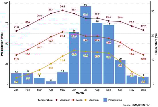
Figure 1.
Climogram of DR 001, Pabellón de Arteaga, Aguascalientes.
2.2. Automated Stations
We used historical data from 22 meteorological stations (Figure 2) of the National Network of Automated Agrometeorological Stations (RNEAA, in Spanish) managed by the National Laboratory of Modeling and Remote Sensing (LNMYSR, in Spanish) of the National Institute of Forestry, Agriculture and Livestock Research (INIFAP, in Spanish). The data cover the period from 1 January 2002 to 31 December 2023 [24].
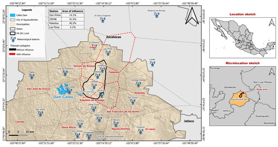
Figure 2.
Location of the meteorological stations.
2.3. Climatol
The Climatol library [25] in the RStudio environment (open-source software, version 2025.090+387) was applied to homogenize and fill in missing data in the climatic series of the selected stations, as well as for quality control. Homogenization was carried out for the following variables in the 22 stations (Figure 3): precipitation (Pr), temperature (maximum, TMAX; minimum, TMIN; and mean, TMEAN), relative humidity (maximum, RHMAX; minimum RHMIN; and mean RHMEAN), solar radiation (SR), and wind speed (WS), at a daily level. Climatol is a robust library that has been successfully applied in other studies. Kuya et al. [26] used Climatol to detect homogeneities in 325 precipitation series in Norway for the period 1961–2018. For their part, Curci et al. [27] used it to construct a homogeneous dataset of temperature and precipitation from 1930 to 2019, on both monthly and daily bases, for the Abruzzo region in Italy.
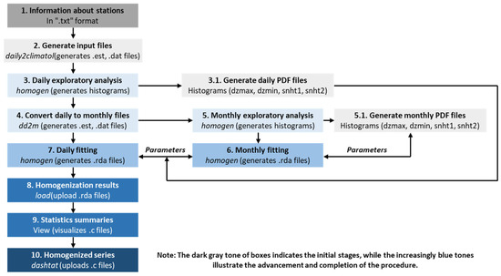
Figure 3.
Homogenization procedure with Climatol.
2.4. Global Climate Models
The Intergovernmental Panel on Climate Change (IPCC) was established in 1988 to comprehensively evaluate scientific information related to CC [28]. Subsequently, the Coupled Model Intercomparison Project (CMIP) provided a standardized framework for climate simulations and projections using GCMs. These numerical models integrate various components of the global climate system, including physical and chemical processes in the atmosphere, oceans, cryosphere, biosphere, Earth’s surface, and radiative interactions [29]. In its sixth phase (CMIP 6) [30], the CMIP includes 134 models developed by 53 research centers. For this study, information was downloaded from the Earth System Grid Federation node, hosted in the Archival and Information Management System and operated by the Lawrence Livermore National Laboratory [31], corresponding to 22 GCMs that contemplate the variables Pr, TMAX, TMIN, TMEAN, SR, RHMAX, RHMIN, RHMEAN, and WS.
The selected projections correspond to the Shared Socioeconomic Paths (SSPs) SSP2-4.5 and SSP5-8.5. Since GCMs operate on a broad spatial scale, they tend to bypass local climate details, leading to biases in simulations. To improve their applicability on the regional scale, we applied a statistical bias correction using quantile mapping (QM) (Figure 4). According to Xu [32] and Bronstert et al. [33], the most relevant climatological variables in studies addressing the impact of CC are precipitation and temperature. However, precipitation poses a greater challenge for climate models due to its high spatio-temporal variability and nonlinear behavior, which introduce greater uncertainty in projections [34].
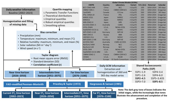
Figure 4.
Methodological framework: bias correction of GCMs through Quantile Mapping (QM), evaluation using Taylor diagrams, and estimation of ET0 across time horizons and SSP scenarios.
The GCM that yielded the highest Pearson correlation coefficient relative to the observed mean precipitation and temperature data was selected. Afterward, ET0 was estimated under the different climate scenarios and time horizons. The model performance was evaluated using the statistical metrics of correlation coefficient (r), standard deviation (sigma, σ and SD), and root mean square error (RMSE), and was visualized using the Taylor Diagram [35].
2.5. Bias Correction
This statistical technique allows the fitting of GCM outputs to correct for systematic biases. The objective is to identify an f transformation function (Equation (1)) that relates the modeled variable for its new distribution to coincide with the distribution of the observed variable [21,36]. The qmap RStudio library is a specialized tool for bias correction in climate data using QM techniques (Figure 5).
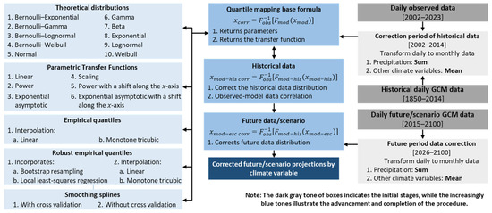
Figure 5.
Procedure for bias correction by QM.
The QM method uses the quantile-quantile relationship to fit the distribution function of the simulated variable to the observed one [36]. By knowing the distribution of the observed variable and applying the probability integral transform [37,38], we obtain:
where F is a Cumulative Distribution Function (CDF) and F−1 is the corresponding quantile function (inverse CDF, F−1). The obs and mod subscripts indicate the distribution parameters that correspond to the observed and modeled data, respectively.
Bias correction was applied only to the Don Primo, CEPAB, Makelisa, and Los Pinos stations, as these were identified—via Thiessen polygons—as having the greatest spatial influence within and around DR 001 (Figure 2). La Mirinda station was excluded due to the high number of missing data points for the study period. For calibration, data from 1 January 2002 to 31 December 2014 were used, as the historical GCM records are only available up to that date.
Since daily data exhibit high variability, making accurate correction difficult [39,40,41], we opted to work with monthly totals for precipitation and monthly averages for all other variables, smoothing out short-term variability. his monthly scale was considered more relevant for long-term ET0 projections and irrigation planning. Nevertheless, to support this decision, we compared results obtained at daily and monthly scales, both before and after bias correction. Each QM method includes several functions; for each GCM, the method and function that achieved the highest correlation between the observed and modeled data ) were selected.
2.5.1. Distribution-Derived Transformations (DIST)
These transformations fit the modeled variable () of Equation (2) from the known theoretical distribution (Figure 5) of the observed variable () [42,43]. The parameters of the distributions are estimated using maximum likelihood methods separately for , from the Probability Density Function (PDF), CDF, and F−1 (Table 1).

Table 1.
Theoretical distributions.
In climate studies, the selection of the theoretical distribution depends directly on the statistical characteristics of each climate variable analyzed; each distribution represents a different degree of fit to the observed data. Studies carried out by Thom [51], Mooley [52] and Cannon [53] on precipitation highlight the fit of combining the Bernoulli distribution, which includes values of zero (dry days), and the Gamma distribution, which models precipitation intensity (suitable for biased data). Other combinations, such as Bernoulli-Lognormal (bernlnorm), Bernoulli-Exponential (bernexp), and Bernoulli-Weibull (bernweibull), are described by Cannon [53], where their PDFs, CDFs, and F−1 are analogous to those described for the Bernoulli-Gamma distribution in Table 1 [44].
2.5.2. Parametric Transfer Functions (PTF)
This parametric method transforms a function (Table 2), characterized by a parameter-oriented frame, to derive the Q-Q relationship [36]. Studies such as those of Piani et al. [54], Dosio & Paruolo [55] and Rojas et al. [56] show consistent results to correct biases in daily global climate simulations of precipitation and temperature by applying the following transformations: linear, exponential asymptotic with a shift along the x-axis, and power with a shift along the x-axis.
Table 2.
Parametric Transfer Functions.
2.5.3. Empirical Quantiles (QUANT) and Robust Empirical Quantiles (RQUANT)
Empirical quantiles, a non-parametric method, estimate the empirical CDF for observed and modeled values in regularly spaced quantiles, rather than assuming parametric or theoretical distributions [21,36,57,58]. In contrast, robust empirical quantiles incorporate a local least-squares linear regression and bootstrap resampling, providing a more robust estimate against outliers [36,44,59,60]. Quantiles are defined from a set of probabilities with step (Table 3).
Table 3.
Mapping of empirical and robust empirical quantiles.
2.5.4. Smoothing Spline (SSPLIN)
It is a non-parametric method, which seeks a smooth function (Equation (3)) that closely approximates the observed and modeled datasets, penalizing excessive curvature to avoid overfitting [61,62]. Where g is estimated to approximate the simulated values to the observed ones (Equation (4)), and the model data is corrected by applying Equation (5).
where is the quantile loss function (also known as the “check” function); is the parameter that controls the balance between the fit and smoothness of the estimated function; determines the rule used in the penalization of the second derivative of , affecting the smoothing shape.
Gudmundsson et al. [21] recommend using the cubic smoothing splines described by Hastie et al. [63]. Enayati et al. [36] mention that few studies utilize splines in variables such as temperature and precipitation, as they display intrinsically different behaviors and characteristics. Within the qmap library, the smoothing parameter is identified by cross-validation (CV-True) or without cross-validation (CV-False) [21].
2.6. Reference Evapotranspiration
ET0 was estimated for the four stations selected based on their spatial representativeness (Thiessen polygons; see Section 2.5), under the SSP2-4.5 and SSP5-8.5 scenarios and across the defined time horizons (Figure 4) using the FAO Penman-Monteith (FAO-56), Priestley-Taylor (P-T), and Hargreaves-Samani (H-S) equations (Table 4).
Table 4.
Reference evapotranspiration equations.
2.7. Monte Carlo Method
To quantify the relative uncertainty and assess consistency between ET0 estimation methods, as well as the robustness of each method against the variability of the input climate variables, the Monte Carlo (MC) method was applied [67]. MC is a non-deterministic technique that uses probabilistic methods and the generation of random numbers to solve complex mathematical expressions, especially those associated with uncertainty, as in the case of GCM projections. Ten thousand simulations were performed.
2.7.1. Uncertainty/Variability in Simulated ET0
For any method that estimates ET0, where represents the input variables in the Monte Carlo simulation (Equation (6)). For each climate variable involved in the ET0 estimating process, the theoretical distribution (Table 1) that best fits its behavior is assigned, based on Akaike [68] goodness-of-fit test. The standard deviation (σ, Equation (7)), confidence interval (CI95%, Equation (8)), and coefficient of variation (CV, Equation (9)) are estimated as follows:
where is the estimated mean; is the number of simulations; is the simulated input vector in iteration .
2.7.2. Analysis of Simulation and Estimate Bias
The mean bias between MC simulations and ET0 values estimated from climate data to determine overestimation/underestimation (Equation (10)), standard deviation (σ, Equation (11)), confidence intervals (CI95%, Equation (12)), and RMSE (Equation (13)) were calculated as follows:
2.8. Sensitivity Analysis
We carried out a Sobol analysis, a variance decomposition technique developed by Sobol [69] that quantifies the sensitivity of an output function with respect to its X inputs, from the fraction of the total variance of each input variable and all combinations. The total variance of the output (Equation (14)), the first-order index (first-order variables, S1, Equation (15)), and the total index (ST, Equation (16)).
where is the variance () due to ; is the variance due to the interaction between and , and so on.
3. Results and Discussion
3.1. Evaluation of GCM Performance on Daily and Monthly Scales
When comparing the performance of the 22 GCMs at two temporal scales—daily and monthly—prior to bias correction, the Taylor diagrams (Figure 6) for the Makelisa station (which has a 40.3% spatial influence within DR 001) show that moving from the daily to the monthly scale increases the correlation, while reducing both the standard deviation (SD) and the root mean square error (RMSE). The only exception is precipitation, for which the SD increases. Overall, the GCMs reproduce long-term means and seasonal patterns more reliably at the monthly scale than at the daily scale, where fluctuations are subject to greater uncertainty and simulation error [70]. Maurer et al. [71] analyzed daily-scale errors in precipitation and temperature from GCMs, concluding that biases are relatively time-invariant, but their daily variability introduces considerable noise. In contrast, monthly aggregation attenuates this variability, allowing the bias to be characterized more stably and thereby improving the robustness of subsequent statistical corrections.
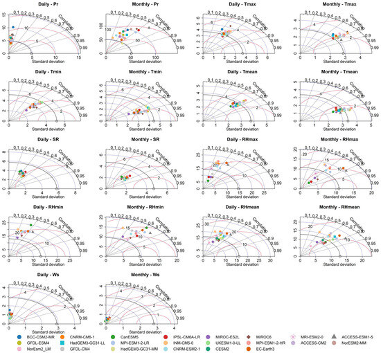
Figure 6.
Comparison of GCM statistical performance at daily and monthly scales before bias correction for the Makelisa station.
Figure 7 shows the quantile–quantile (Q–Q) plots for daily and monthly scales of the ACCESS-ESM1-5 model, developed by the CSIRO Laboratory in Australia. As indicated in the Taylor diagrams, this model consistently emerges as the one with the highest correlation among the 22 GCMs. The Q–Q analysis reveals clear differences in precipitation distributions across scales. At the daily scale, quantiles between 0 and 45% take values equal to zero, indicating that approximately half of the days are dry in both the observations and the model. The fit at the extremes is relatively good, with a maximum observed daily value of 79.8 mm compared to 74.0 mm from the model, corresponding to an underestimation of approximately 7%. At the monthly scale, however, the distribution shifts notably: almost all months present rainfall, and the biases are amplified. In the central quantiles, model accumulations exceed observations by approximately 3.0–4.0 times on average, a pattern also visible at the extremes. These results indicate that small daily discrepancies in intensity and frequency accumulate into a systematic and substantial overestimation of monthly totals.
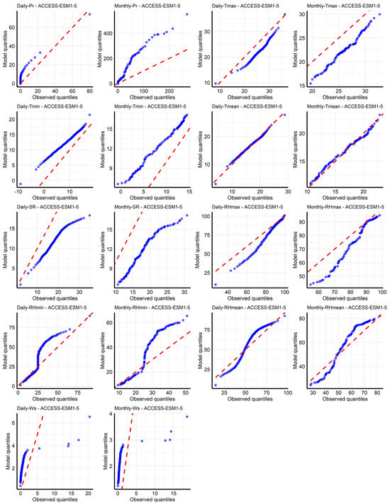
Figure 7.
Q–Q plots of the ACCESS-ESM1-5 model at daily and monthly scales for the Makelisa station. The red line represents the 1:1 relationship, while the blue dots show the data distribution.
The Q–Q plots showed that for the three temperature variables (TMAX, TMIN, TMEAN), the ACCESS-ESM1-5 model maintains a systematic bias across the full range of quantiles, characterized by an underestimation of maximum and mean temperatures and an overestimation of minimum temperatures. These biases remain consistent when transitioning from the daily to the monthly scale, although cold and warm extremes are attenuated, resulting in smoother distributions and more uniform biases. This pattern facilitates the application of bias correction methods, but it may also conceal short-duration extreme events. Therefore, the use of monthly data for ET0 estimation under long-term projections is appropriate for this study [72,73].
For relative humidity (RHMAX, RHMIN, RHMEAN), monthly aggregation reduces the dispersion of distributions—minimum values increase and maximum values decrease—yet structural biases remain. Maximum humidity and the lower tails of minimum and mean humidity are generally underestimated, while central quantiles of minimum and mean humidity show persistent overestimation. In summary, the transformation from daily to monthly significantly reduced noise and produced more homogeneous biases, thereby facilitating bias correction for long-term climate applications.
SR and WS also exhibit systematic biases at the daily scale, with radiation being strongly underestimated and low-intensity winds overestimated, as well as an underrepresentation of extremes. Aggregation to the monthly scale reduces dispersion but does not fully resolve these biases. Thus, results should be interpreted with the understanding that the monthly approach adequately represents long-term trends and climatological means, but not sub-daily variability or the occurrence of peak extremes [72,73].
Table 5 presents the bias of each climate variable for the four selected stations across low, middle, and high quantiles, where positive values indicate an overestimation by the ACCESS-ESM1-5 model and negative values indicate an underestimation.
Table 5.
Bias between observed and modeled quantiles before correction.
In summary, ACCESS-ESM1-5 reproduces temperature and radiation with relatively high fidelity, whereas humidity and wind remain more uncertain. These findings support our decision to transform daily data to the monthly scale prior to applying QM for bias correction, given that the ultimate objective is to estimate ET0 across different time horizons (2026–2050, 2051–2075, 2076–2100), where the aggregated behavior of the variables is more relevant than daily fluctuations. Athira et al. [74] further demonstrated that averaging meteorological inputs at weekly or monthly scales before running ET0 estimation models reduces RMSE compared to averaging daily model outputs.
3.2. Evaluation of GCM Performance Before and After Bias Correction at Daily and Monthly Scales
After applying bias correction using QM at both daily and monthly scales, changes were mainly observed in the magnitude of variability among the GCMs. This adjustment allowed the standard deviation (SD) of most models to align with that of the historical reference period (2002–2014) and reduced the RMSE, as shown in Figure 8. Although QM satisfactorily adjusted the distribution of GCM data, the procedure did not produce significant changes in the correlation coefficient—an expected result, since the correction is applied to the marginal distribution of the variables without modifying their temporal order or the synchronicity of events.
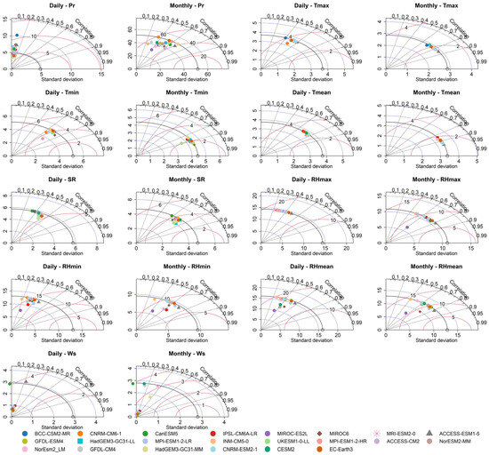
Figure 8.
Comparison of the statistical fit between the daily and monthly scales after bias correction for the Makelisa station.
After applying bias correction and re-plotting the Q–Q diagrams for the Makelisa station (Figure 9 and Figure 10), the results showed a closer alignment to the 1:1 line for most variables. For precipitation (Pr), a better fit to the 1:1 line was observed at the monthly scale with the ACCESS-ESM1-5 model, which had previously shown the highest correlation. In contrast, at the daily scale, the best performance corresponded to the MPI-ESM1-2-LR model. This suggests that temporal aggregation can influence model representativeness. For minimum temperature (TMIN), the correction identified MIROC6 as the model with the best fit at both temporal scales, outperforming the previously identified ACCESS-ESM1-5, particularly by improving the fit of the lower quantiles.
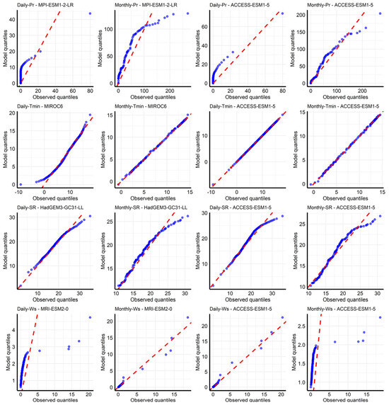
Figure 9.
Q–Q comparison: optimal models (left) vs. ACCESS-ESM1-5 model (right) after bias correction for the Makelisa station. The red line represents the 1:1 relationship, while the blue dots show the data distribution.
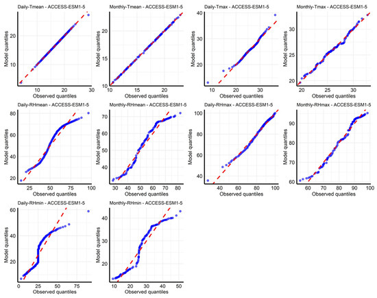
Figure 10.
Variables that retained ACCESS-ESM1-5 as the optimal model after bias correction for the Makelisa station. The red line represents the 1:1 relationship, while the blue dots show the data distribution.
For SR, quantile fitting improved after correction. At the daily scale, ACCESS-ESM1-5 remained the best-performing model, while at the monthly scale, HadGEM3-GC31-LL became optimal, reflecting that the variability of this variable may be better captured in aggregated series. WS exhibited heterogeneous behavior: at the monthly scale, the best-performing models varied among stations, while at the daily scale, ACCESS-ESM1-5 remained optimal for the stations with the greatest regional influence.
For TMEAN and TMAX, ACCESS-ESM1-5 remained the optimal model after correction at both scales, with TMAX showing a particularly improved fit in the extreme quantiles at the monthly scale. Relative humidity variables (RHMEAN, RHMAX, RHMIN) also retained ACCESS-ESM1-5 as the optimal model before and after correction at both temporal scales. However, while RHMEAN and RHMAX showed an overall improvement in fit, they continued to struggle with accurately representing extreme quantiles.
Finally, RHMIN exhibited a mixed pattern: overestimation at lower quantiles, underestimation at higher quantiles, and variable behavior in the central range. Although not all climate variables in ACCESS-ESM1-5—the model with the best pre-correction correlation—remained optimal after adjustment, the differences between ACCESS-ESM1-5 and the newly selected models were generally small across most quantiles. This suggests that the changes primarily reflect fine-scale enhancements in variability representation rather than fundamentally different behavior.
Therefore, using all variables from ACCESS-ESM1-5 to estimate ET0 is considered appropriate. The boxplots in Figure 11, comparing daily and monthly scales, show that although the median and interquartile range of the variables remain similar between the two series, the whiskers are shorter and the number of outliers decreases drastically at the monthly scale.
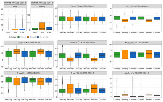
Figure 11.
Distribution of the ACCESS-ESM1-5 model: comparison between daily and monthly scales for the Makelisa station.
This indicates that temporal aggregation did not compromise the underlying climate signal, as it did not distort the trends of the series. By reducing the influence of extremes and stabilizing the distribution, aggregation favored a more consistent performance of the bias correction methods [72]. Overall, these findings support the decision to work at the monthly scale for ET0 estimation in future projections (2026–2100), as it provides a statistically more stable and suitable representation for analyzing long-term climate changes. Consequently, the results presented below focus exclusively on the monthly scale.
Table 6 summarizes the climate variables analyzed for the stations with the greatest spatial influence on DR 001, as well as the bias correction method that achieved the highest correlation with the observed data at each scale.
Table 6.
GCM and the method that achieved the highest correlation after bias correction.
3.3. Precipitation
In both in the global analysis between models and the model with the highest individual correlation, the PTF method, especially the scale function, showed superior performance in the correction process, given the high spatial and temporal variability of precipitation [34,75,76], which coincides with what Vigna et al. [77] reported for this variable. However, performance may vary depending on the region and time scale considered. In their analysis of the Karkheh River Basin, Iran, Enayati et al. [36] found that the RQUANT and QUANT methods performed better than PTF. The ACCESS-ESM1-5 model yielded the best correlation, which reinforces the spatial consistency of the good performance of the PTF-scale method.
Figure 12 shows the projected variations for Pr under the scenarios SSP2-4.5 and SSP5-8.5, differentiated by time horizon (near, intermediate, and far) and seasonal period (SP)—autumn–winter (A–W) and spring–summer (Sp–S)—and annual average. A reduction trend is observed for A–W, and an increase for Sp–S, in seasonal water availability in DR 001 compared to the baseline period. These changes are more moderate under the SSP5-8.5 scenario and more pronounced under the SSP2-4.5 scenario. The maps of the spatio-temporal distribution of climate variables are shown in Appendix A. In particular, Figure A1 shows that Pr is affected to a greater extent in the central area of DR 001.
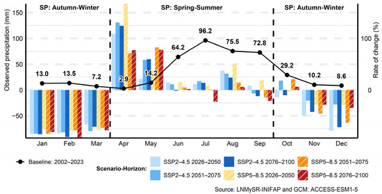
Figure 12.
Rate of change by scenario-horizon for Pr.
3.4. Temperature
The selection of different QM correction methods depending on the temperature variables—TMEAN, TMAX, and TMIN—reflects the differences in the descriptive statistics of these variables, as well as the way each method adapts to their particular distributions. This allows us to evaluate its effectiveness in a differentiated manner for DR 001, where the projections show more moderate temperature increases under the SSP2-4.5 scenario and more pronounced under SSP5-8.5. It should be noted that, of the 22 GCMs used, the CESM2 model does not report values for TMAX and TMIN.
Figure 13, Figure 14 and Figure 15 show the projections of the variation for TMEAN, TMAX, and TMIN under the scenarios SSP2-4.5 and SSP5-8.5, considering the different time horizons. For TMEAN and TMAX, the most significant increases are recorded during the autumn–winter (A–W) period, while for TMIN they are observed in spring–summer (Sp–S), with relatively moderate values in the SSP2-4.5 scenario and more pronounced in SSP5-8.5.
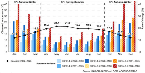
Figure 13.
Rate of change by scenario-horizon for TMEAN.
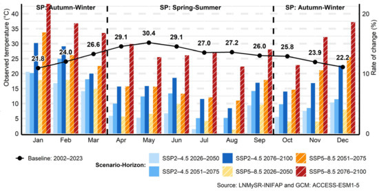
Figure 14.
Rate of change by scenario-horizon for TMAX.
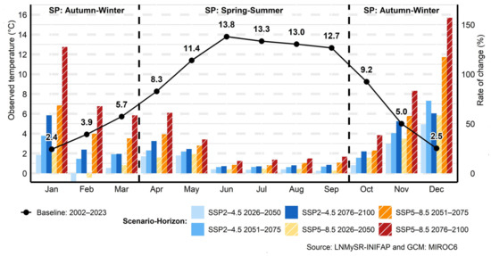
Figure 15.
Rate of change by scenario-horizon for TMIN.
3.4.1. Mean Temperature
For TMEAN, the RQUANT method, with the linear and tricub functions, showed the best overall performance among GCMs, as its greater robustness allowed it to fit the distribution without depending on a specific function. However, the method with the highest correlation between stations was QUANT, whose statistical structure was most similar to the observations. The daily TMEAN typically exhibits a symmetrical and smoothed distribution, resulting from averaging the daily maximum and minimum values, which eliminates many outliers and reduces the variance. Therefore, these correction methods are particularly suitable for temperature variables [36,78,79]. The ACCESS-ESM1-5 model showed the best correlation in the four meteorological stations, confirming the spatial consistency of the QUANT method in three of them. TMEAN typically exhibits less noise and asymmetry than other climate variables; the QUANT method managed to flexibly fit the observed data without requiring an explicit mathematical function. This underscores its suitability for variables with smooth and symmetrical distributions, such as daily TMEAN.
3.4.2. Maximum Temperature
For TMAX, the predominant correction method globally was PTF, with the power and power.x0 functions. However, the estimated correlation coefficients for TMAX (0.68–0.87) were lower than those for TMEAN (0.83–0.95) and TMIN (0.82–0.94). This difference may be due to its distribution having a long tail resulting from the greater daily variability driven by local factors such as cloud cover, wind conditions, or direct SR.
Studies such as that of Enayati et al. [36] highlight that methods like PTF and SSPLIN have limitations, mainly regarding extreme values. This high variability makes it difficult for GCMs to accurately represent extreme values, which in turn reduces the effectiveness of correction methods. Previous research that employed one or more of the GCMs used in this analysis, e.g., [80,81,82,83,84], has shown the difficulties of these models to adequately simulate extreme events, showing a tendency to overestimate or underestimate them, particularly at high spatial resolutions. Due to its high variability and sensitivity to fast-fluctuating local factors, TMAX poses greater challenges for accurate representation. Although the corrections applied can improve the simulations, significant discrepancies in the reproduction of extreme values remain [85]. The model that showed the highest post-correction correlation was ACCESS-ESM1-5. These results indicate an improvement in the representation of variability relative to the observations.
3.4.3. Minimum Temperature
While the predominant global method was RQUANT for TMEAN and PTF (power and power.x0) for TMAX, it was the SSPLIN method for TMIN, followed by PTF. However, Enayati et al. [36] note that PTF and SSPLIN may show limitations when correcting extreme values, while RQUANT and QUANT are generally more effective in reducing bias for temperature variables [36,86,87]. The GCM that returned the best correlation with the observations after bias correction was MIROC6 (developed by the MIROC laboratory in Japan).
This indicates that this model already adequately represents nocturnal variability, allowing the RQUANT (linear) and QUANT (tricub) correction methods to be sufficient for achieving an adequate fit. The ACCESS-ESM1-5 model was not the best, as for TMEAN, TMAX, and Pr, but it was ranked among the three best-performing models, with correlation coefficients ranging from 0.91 to 0.93, close to that of MIROC6 (0.94). This finding suggests that the model is robust and reliable, accurately simulating the observed conditions.
Figure A2, Figure A3 and Figure A4 show the spatio-temporal distribution of TMEAN, TMAX and TMIN, respectively, within DR 001, revealing a gradual increase toward the southern zone. The northern zone reaches values comparable to those of the south as projections move toward the far horizon. The central zone also exhibits increases, although to a lesser extent, suggesting a more moderate response to climate change.
3.5. Solar Radiation
The primary correction method, both globally and in the model with the highest correlation, was PTF (linear and scale), the latter being the one that achieved the best performance in the correction process, positioning itself as the method with the highest fit precision. In the case of Pr, PTF-scale was also the method with the highest correlation, which can be attributed to the fact that SR and Pr share similar statistical characteristics, such as a right-biased distribution, characterized by a high frequency of low values and a lower frequency of extreme values. SR reaches its maximum values under clear sky conditions and decreases considerably on cloudy days, as clouds introduce complex spatial patterns at very small scales, which significantly affect SR variability [88].
GCMs adequately simulate SR values under clear sky conditions but show inaccuracies on cloudy days due to the complexity of the physical processes involved in cloud formation and evolution. These processes are often simplified in GCMs to reduce the computational load, compromising the accuracy of simulations under cloudy conditions [89,90]. This complexity in representing cloud cover limits the ability of bias correction methods to reach high correlation values with observations.
After correction, the GCM that yielded the best correlation with observed data was HadGEM3-GC31-LL (developed by the Met Office Hadley Centre, MOHC, United Kingdom), demonstrating the spatial consistency of the PTF-scale method. ACCESS-ESM1-5 also ranked among the three best-performing models, with correlation coefficients from 0.63 to 0.79, very close to the values obtained with the best-performing model (0.67 to 0.79). This suggests that ACCESS-ESM1-5 maintains a robust ability to simulate the observed variability of SR.
Figure 16 describes the projected changes in SR under the SSP2-4.5 and SSP5-8.5 scenarios, differentiated by time horizons and seasons. The results indicate both increases and occasional decreases—especially in October —compared to the baseline scenario. The projected values are more moderate under SSP2-4.5 and more pronounced under SSP5-8.5. During the Sp–S period, increases in SR are more pronounced than in A–W. Annually, increases of 6.6% to 8.1% are projected for SSP2-4.5 and of 7.1% to 9.5% for SSP5-8.5, confirming a more pronounced upward trend in the higher-GHG- concentration scenarios. These changes can significantly impact cumulative ET0, which, in the long term, translates into a significantly greater irrigation demand in agricultural areas such as DR 001.
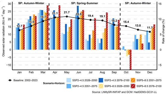
Figure 16.
Rate of change by scenario-horizon for SR.
Figure A5 illustrates the spatio-temporal distribution of SR within DR 001, characterized by a gradual increase in the southern and northern zones, with a greater spatial coverage of these increases in the different time horizons and scenarios evaluated. This pattern is consistent with that observed for TMEAN, where increases in SR are observed in the central zone, although of lesser magnitude compared to the southern and northern regions.
3.6. Relative Humidity
The predominant selection of a correction method according to the type of relative humidity—RHMEAN, RHMAX, and RHMIN—reflects similarities in the descriptive statistics of these variables and their correspondence with the statistical assumptions of each correction method, which allows evaluating their effectiveness in DR 001. Of the 22 models considered, BCC-CSM2-MR does not provide RHMEAN data, and only 14 models contain information on RHMAX and RHMIN.
Figure 17, Figure 18 and Figure 19 show projections of changes in RHMEAN, RHMAX, and RHMIN at seasonal and annual levels under the SSP2-4.5 and SSP5-8.5 scenarios. And Figure A6, Figure A7 and Figure A8 illustrate the spatio-temporal distribution of RHMEAN, RHMAX and RHMIN, respectively, showing that the southern zone experiences a progressive decrease throughout the different time horizons and scenarios.
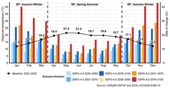
Figure 17.
Rate of change by scenario-horizon for RHMEAN.
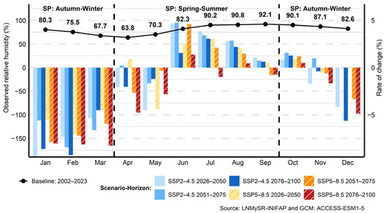
Figure 18.
Rate of change by horizon-scenario for RHMAX.
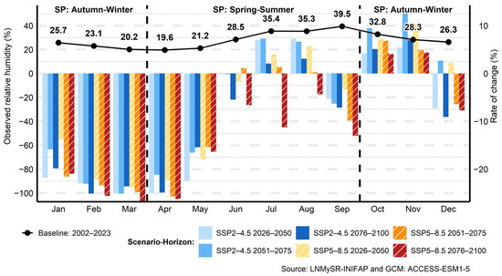
Figure 19.
Rate of change by scenario-horizon in RHMIN.
At the annual level, the three variables exhibit reductions, being more moderate under the SSP2-4.5 scenario and more accentuated in SSP5-8.5. Relative humidity tends to decrease as a result of the increase in air temperature, since the latter translates into a higher water vapor retention capacity of the atmosphere. However, if the increase in the absolute amount of vapor is not proportional, the relative humidity drops because the saturation capacity increases at a faster rate than humidity [91].
3.6.1. Mean Relative Humidity
The correction showed that, for RHMEAN, the predominant overall method was PTF (linear, power.x0, and scale). However, after correction, just over one-half of the GCMs returned a correlation coefficient lower than 0.70 and an RMSE above 10.0. The ACCESS-ESM1-5 model, combined with the PTF method (linear and power.x0), achieved the best correlations for RHMEAN (0.80–0.82), indicating the spatial consistency of the performance of the PTF method across the four stations. As it is a smoothed value resulting from the integration of measurements over a full day (daily average), RHMEAN shows less variability and retains a near-normal distribution [92].
As it depends on TMEAN and water vapor content, it is less susceptible to extreme errors, making it easier for GCMs to generate more accurate simulations and allowing for a more effective correction for RHMEAN than for RHMAX and RHMIN [93]. A more pronounced decrease in RHMEAN is evident during the A–W period, while more significant increases in RHMAX are observed during Sp–S.
3.6.2. Maximum Relative Humidity
The RQUANT-tricub, PTF-linear, and SSPLIN-CV-False methods showed the best overall fits in RHMAX. The ACCESS-ESM1-5 model achieved the best correlation in the four stations, indicating the spatial consistency of the PTF-linear method, with correlation coefficients of 0.78 to 0.83, similar to those obtained for RHMEAN. However, over one-half of the GCMs returned a correlation coefficient below 0.70 and an RMSE above 10.0, indicating that several GCMs achieve a limited accuracy, even after correction.
3.6.3. Minimum Relative Humidity
For RHMIN, the PTF-scale method yielded the best fit, albeit with lower correlation values (0.72–0.75) than for RHMEAN (0.80–0.82) and RHMAX (0.78–0.83). RH is influenced by specific events such as localized rainfall, sudden cloudiness, or abrupt temperature variations, the latter being a key factor due to its high correlation with humidity [14,91]. As indicated previously, GCMs have limitations in adequately simulating the values of TMAX and TMIN, which translates into greater propagation of error in RHMAX and RHMIN projections, since these variables are closely related to temperature.
3.7. Wind Speed
In general, the PTF-scale method achieved the best performance in Don Primo, with a correlation coefficient of 0.34. The other methods, i.e., QUANT-tricub, RQUANT-linear, and SSPLIN-CV-True, showed a better fit, with coefficients ranging from 0.36 to 0.47. This suggests that the performance of PTF-scale for WS may vary depending on the local conditions or the quality of observed data. This reflects the difficulty of GCMs in adequately simulating wind conditions, which are strongly influenced by local factors. As a result, QM correction fails to sufficiently represent the spatio-temporal variability, suggesting that more advanced statistical models or machine-learning techniques should be used to obtain better results. MRI-ESM2-0 (developed at the MRI Laboratory in Japan) was the best-performing model in two of the four stations. In contrast, ACCESS-ESM1-5, which demonstrated outstanding performance for Pr, TMEAN, TMAX, RHMEAN, RHMAX, and RHMIN, did not maintain the same fit level for WS, ranking among the top three models in two stations but showing a lower performance in the remaining ones. Figure 20 shows both increases and decreases relative to the baseline scenario, with more moderate values in SSP2-4.5 and higher values in SSP5-8.5, especially during the Sp–S period.
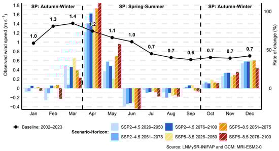
Figure 20.
Rate of change by scenario-horizon for WS.
A greater increase in WS is observed in Sp–S than in A–W. On an annual basis, increases are most pronounced under SSP5-8.5 in the near and intermediate horizons. In contrast, for the far horizon, the SSP2-4.5 scenario shows the greatest increase in WS.
For this variable, the correlation coefficients were low, attributed to the asymmetric distribution of WS, with long tails and extreme events, resulting in a scarcity of representative data at the extremes of the distribution. As a result, bias correction tends to add uncertainty by magnifying the trends in extreme values and distorting the spatial and temporal structure of the corrected data. This distortion is especially pronounced when fitted at local scales, given that WS exhibits a high variability, both spatially and temporally [94,95,96]. Figure A9 shows the spatio-temporal distribution of WS within DR 001, evidencing regional variations that reflect the influence of local conditions on future projections.
3.8. Validation of the ACCESS-ESM1-5 Model Against the Multi-Model Ensemble
After applying bias correction to the eight climate variables used to calculate ET0, the ACCESS-ESM1-5 model achieved the best performance for six of them—TMEAN, TMAX, TMIN, RHMEAN, RHMAX, and RHMIN—across the four stations evaluated, returning high correlation coefficients and low RMSE values. For SR and WS, the model ranked second and fourth, respectively, while it ranked first for Pr. Based on these results, ACCESS-ESM1-5 was selected as the reference model to estimate ET0 in DR 001.
To evaluate structural uncertainty in the ET0 projections, we compared ACCESS-ESM1-5 outputs with a multi-model ensemble (MME) constructed from the bias-corrected GCMs. This comparison was performed only for projections estimated with the FAO-56 method, as it incorporates the largest number of climate variables. Figure 21 shows the dispersion bands of the MME (p5–p95 and p25–p75), with the median as the central reference. The median was chosen over the mean due to its robustness against extreme values, which is particularly relevant given that some models overestimate ET0.
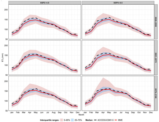
Figure 21.
Comparison of ET0 projections from the MME and the ACCESS-ESM1-5 model using the FAO-56 method.
The comparison shows that ACCESS-ESM1-5 closely follows the ensemble’s central tendency. From January to June, the model projects slightly higher values than the MME median across all horizons and scenarios, often lying near the upper bound of the interquartile range (p25–p75). This indicates that ACCESS-ESM1-5 tends to project relatively high ET0 values within the typical range of most models. From July to December, the model positions itself slightly below or coincides with the MME median.
Figure 22, through the monthly boxplots of the MME by scenario, further confirms that ACCESS-ESM1-5 values generally fall within the ensemble’s interquartile range. This demonstrates that the model’s behavior follows the inter-model spread and does not deviate substantially from the majority of projections.
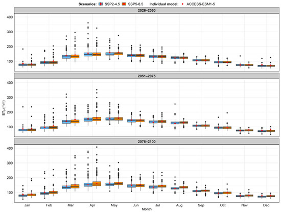
Figure 22.
Multi-model ensemble variability of monthly ET0 vs. ACCESS-ESM1-5 for FAO-56.
Overall, these results suggest that ACCESS-ESM1-5 can reliably capture the MME’s central tendency, although it is essential to acknowledge that the multi-model ensemble provides additional insight into structural uncertainty. Therefore, while relying exclusively on ACCESS-ESM1-5 is justified insofar as its projections align with the ensemble’s median and spread, ensemble comparisons remain valuable for contextualizing inter-model variability.
3.9. ET0 Estimates in Time Horizons
After bias correction was applied to the eight climate variables used to calculate ET0, the ACCESS-ESM1-5 model showed the best performance for six of them—TMEAN, TMAX, TMIN, RHMEAN, RHMAX, and RHMIN—in the four stations evaluated, returning high correlation coefficients and low RMSE values. For SR and WS, the model reached the second and fourth positions, respectively, while it ranked first for Pr. Based on these results, ACCESS-ESM1-5 was selected as the final model to estimate ET0 in DR 001.
Figure 23, Figure 24 and Figure 25 illustrate the projected behavior of ET0 calculated using the FAO-56, P-T, and H-S methods, respectively, throughout the year. During the periods A–W and Sp–S, increases in ET0 are projected under both climate scenarios, with more moderate values under the SSP2-4.5 scenario and higher values under the SSP5-8.5 scenario.
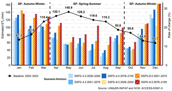
Figure 23.
Rate of change by scenario-horizon for ET0 estimates with the FAO-56 method.
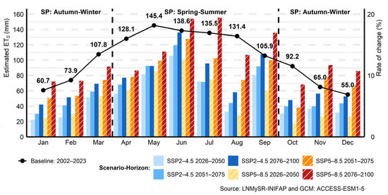
Figure 24.
Rate of change by scenario-horizon for ET0 estimates with the P-T method.
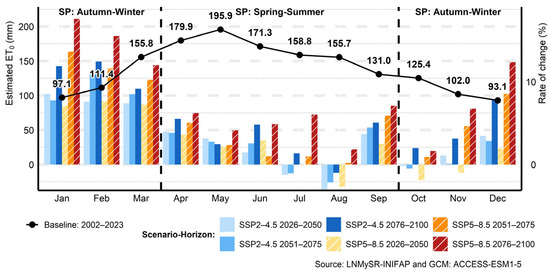
Figure 25.
Rate of change by scenario-horizon for ET0 estimates with the H-S method.
Estimates using the FAO-56 method show a greater increase in A–W, with ranges between 16.5% and 24.1%, while P-T shows its greatest increase in Sp–S, from 8.7% to 15.6%. On the other hand, H-S shows higher absolute values compared to FAO-56 and P-T, but with more moderate increases under both scenarios, from 1.4% to 10.7%, attributed to its lower sensitivity to certain climate variables. This behavior is consistent with the findings reported by Monterroso-Rivas & Gómez-Díaz [14], who concluded that ET0 will increase throughout the national territory as a result of the rise in air temperature (Figure 13, Figure 14 and Figure 15) and the decrease in relative humidity (Figure 17, Figure 18 and Figure 19).
Figure 26, Figure 27 and Figure 28 show the spatial and temporal distribution of ET0 estimated using the FAO-56, P-T, and H-S methods. FAO-56 and P-T produced a similar spatial pattern, with the highest ET0 values in the southern zone, followed by the northern zone, and the lowest values in the central zone. This behavior remains constant throughout the different time horizons and between the two climate scenarios considered, with more moderate values under SSP2-4.5 and higher values under SSP5-8.5, indicating a gradual increase in evaporative demand derived from CC across DR 001. Unlike the FAO-56 and P-T methods, H-S shows a more homogeneous distribution of ET0 in the current scenario. However, as time horizons advance, a more marked increase is observed in the northern zone than in the southern zone. This trend is accentuated on the far horizon under both climate scenarios (SSP2-4.5 and SSP5-8.5), indicating a likely spatial redistribution of the increase in evaporative demand as CC progresses.
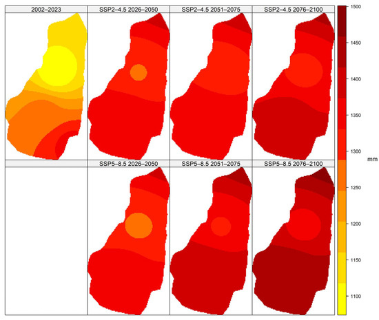
Figure 26.
Spatio-temporal variation by scenario-horizon for ET0 estimates with the FAO 56 method.
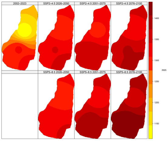
Figure 27.
Spatio-temporal variation by scenario-horizon for ET0 estimates with the P-T method.
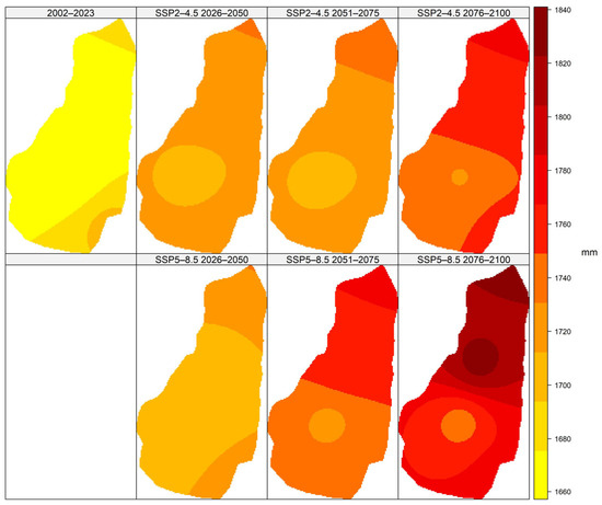
Figure 28.
Spatio-temporal variation by scenario-horizon for ET0 estimates with the H-S method.
Previous studies at the international level have also reported increases in ET0 by the end of this century. This prediction aligns with the results of this study using the ACCESS-ESM1-5 model, which estimated increases in all the time horizons evaluated. For example, on a global scale, Liu et al. [97] compared projections from the CMIP5 and CMIP6 models, concluding that CMIP6 models—including ACCESS-ESM1-5—project greater increases in ET0, mainly in arid and semi-arid regions.
Similarly, Yahaya et al. [98] based on the assembly of 20 CMIP6 models, projected an increase of 0.23 mm year−1 in ET0 for Africa by 2100 under the SSP5-8.5 scenario. Similarly, Muhammad et al. [99] found that, in Malaysia, ET0 would increase by up to 21% between 2070 and 2099, compared to its 1970–1999 baseline. In China, Zhang et al. [100] projected increases of between 8% and 14% by the year 2100.
Other studies, such as those of Maqsood et al. [101] and Bellido-Jiménez et al. [102] also estimated significant increases in ET0, of between 9.7% and 18.4% by the year 2100 under the RCP4.5 and RCP8.5 scenarios, respectively, using CMIP5 models, with the most noticeable increases under RCP8.5, especially in Canada and southern Spain.
3.10. Analysis of Uncertainty and Bias in ET0
Table 7 presents the estimate of the internal uncertainty of ET0 calculation methods. The FAO-56 method produced the lowest uncertainty in the four DR 001 stations, with a CV between 8.99% and 10.32%, and a CI range between 0.94 and 1.05 mm day−1. These results indicate that the FAO-56 method is more robust against simulated climate variability than the P-T (CV: 13.09–13.43%) and H-S (CV: 16.80–16.99%) methods.
Table 7.
Uncertainty in MC simulations for 2002–2023.
This lower uncertainty in FAO-56 estimates supports its greater physical complexity, as it considers the energy balance as well as aerodynamic and stomatal resistance, making it less sensitive to random fluctuations. This was demonstrated by Kadkhodazadeh et al. [103] using a machine-learning approach and Monte Carlo simulations to assess future uncertainty in ET0 under different climate scenarios. Other studies, such as that of Wang & Wang [104], also showed that the use of stochastic simulations combined with CMIP models facilitates the identification of ET0 estimation methods that are more resilient to projected climate uncertainties.
This reinforces their reliability in CC contexts, as also suggested by Papalexiou et al. [105] and Egli et al. [106], note out that integrating models with more complete physical foundations contributes to minimizing the propagation of uncertainty in future probabilistic analyses. Figure 29 shows the degree of bias in simulations compared to ET0 estimates obtained with the different methods. At the Don Primo and CEPAB stations, the P-T method showed the virtual absence of a negative bias (slight underestimation), although with less precision.
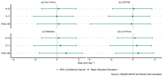
Figure 29.
95% CI for ET0 bias, period 2002–2023.
On the other hand, H-S showed positive bias (tendency to overestimate), lower variability, a narrower confidence interval (higher precision), and the lowest RMSE across the methods evaluated. In contrast, FAO-56 recorded the highest variability and the highest RMSE, indicating less consistency in its estimates. In Makelisa and Los Pinos, H-S was the method with the lowest bias and highest precision, followed by P-T, while FAO-56 recorded the highest bias and lowest precision. The FAO-56 method exhibited lower uncertainty (lower sensitivity) to the variability of input variables, which makes it a more stable and consistent option in future scenarios; however, it produced a higher absolute error in the estimates.
On the other hand, P-T and H-S showed a lower bias, as their estimates were closer to the reference values, which makes them more accurate options in terms of error. These results are consistent with the findings of Dobrovolski et al. [107], who identified a greater sensitivity in the stochastic response of ET0 when simplified formulas, such as P-T and H-S, are used. However, both methods were also more susceptible to variations in simulated climatic conditions, leading to greater dispersion and uncertainty.
3.11. Sobol Analysis for ET0
Figure 30 shows that, for the FAO-56 method, the variables with the greatest influence on ET0 estimates are SR, which explains between 43% and 56% of the variability (S1) and between 42% and 55% of the total variance (ST); the Julian day (JD), that determines extraterrestrial radiation (Ra), explaining between 22% and 33% (S1) and 21% to 32% (ST); and WS, with a contribution of 12% to 19% (S1) and 13% to 19% (ST). For the P–T method, the most influential variables were SR and JD, with contributions of 53% to 68% and 27% to 41% (S1), respectively.
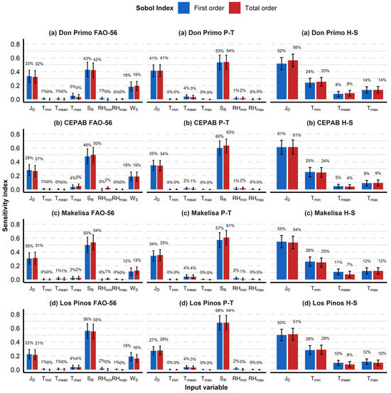
Figure 30.
Sobol Sensitivity Indices for ET0.
Finally, for H–S, the variables with the greatest impact were JD and TMIN, which dominate ET0 estimation. Studies such as those by Sabino & de Souza [108] in the state of Mato Grosso, Brazil, and Ha et al. [109] in the province of Gia Lai, Vietnam, showed that ET0 is more sensitive to SR and day length, which depend on the Julian day (JD). However, studies such as Guo et al. [110] in different climatic zones of Australia, Cao et al. [111] in various climatic zones of China, and Biazar et al. [112] in a humid region of Iran, reported that temperature was the most influential variable, followed by SR, while RH and WS showed the lowest influence. These results highlight that the relative contribution of each variable can vary significantly depending on the geographical context, underscoring the importance of considering local conditions when estimating ET0.
4. Conclusions
This study evaluated the impact of climate change on the reference evapotranspiration (ET0) in DR 001, showing that future scenarios project significant increases that represent a negative impact by intensifying crop water demands and placing additional pressure on water availability and management. The assessment was based on projections from 22 GCMs, corrected for bias under the SSP2-4.5 and SSP5-8.5 climate scenarios.
The results show that the application of statistical correction methods significantly improves the representativeness of the simulations compared to the observed data, which strengthens the reliability of regional projections. Despite the limitations for highly sensitive variables such as Pr, RH, and WS, the study demonstrates that adequate selection of the correction method significantly improves the quality of input data for calculating ET0.
The uncertainty and bias analysis using Monte Carlo simulations showed that, although the FAO-56 method produced greater uncertainty under current conditions, it was more robust and reliable in future scenarios, in contrast to the P-T method, which was more accurate in the historical period. These findings indicate that FAO-56 is the best method for long-term projections. The Sobol sensitivity analysis identified sun radiation (SR), wind speed (WS) and Julian day (JD) as the variables with the greatest independent influence on FAO-56 and P-T, which facilitates their application in contexts of high climatic uncertainty.
Among the 22 GCMs evaluated, ACCESS-ESM1-5 achieved the best overall performance after bias correction, exhibiting high consistency with observations and maintaining an adequate balance in key variables such as SR, Pr, and TMEAN. This makes it a reliable tool for generating regionalized climate scenarios in semi-arid agricultural areas, such as DR 001. Finally, a gradual increase in ET0 is projected in both climate scenarios. In SSP2-4.5, ET0 ranges from 17.7% to 20.3% and intensifies towards the end of the century (2081–2100); in SSP5-8.5, it ranges from 16.5% to 24.1%, being more severe in all time horizons, especially in autumn–winter.
This trend implies greater pressure on the water demand of the agricultural system and highlights the urgent need to implement local water adaptation strategies. Together, these findings establish a solid technical basis for more efficient and resilient water resource management and contribute to the design of adaptive public policies in the face of CC in vulnerable agricultural regions.
Author Contributions
Conceptualization, O.G.-C. and M.A.B.-G.; methodology, M.A.B.-G. and O.G.-C.; software, O.G.-C. and M.A.B.-G.; validation, M.A.B.-G. and O.G.-C.; formal analysis, M.A.B.-G. and O.G.-C.; investigation, O.G.-C., M.A.B.-G., A.A.E.-G., A.L.-P., J.V.P.-H. and G.C.-G.; resources, M.A.B.-G.; data curation, O.G.-C. and M.A.B.-G.; writing—original draft preparation, O.G.-C. and M.A.B.-G.; writing—review and editing, O.G.-C., M.A.B.-G., A.A.E.-G., A.L.-P., J.V.P.-H. and G.C.-G.; visualization, O.G.-C. and M.A.B.-G. All authors have read and agreed to the published version of the manuscript.
Funding
This study was financed by the Consejo Nacional de Humanidades, Ciencias y Tecnologías (CONAHCYT) for funding the Ph.D. studies of O.G.-C. (Scholarship no. 789301).
Data Availability Statement
Dataset available upon request from the authors.
Acknowledgments
The authors wish to thank the CONAHCYT, as well as the Hydrosciences Postgraduate Course of the Colegio de Postgraduados, for the support provided in the development of this research study. María Elena Sánchez-Salazar translated the manuscript into English.
Conflicts of Interest
The authors declare no conflicts of interest.
Abbreviations
The following abbreviations are used in this manuscript:
| DR 001 | Irrigation District 001 Pabellón de Arteaga, Aguascalientes |
| Pr | Precipitation |
| TMAX | Temperature maximum |
| TMIN | Temperature minimum |
| TMEAN | Temperature mean |
| SR | Solar radiation |
| RHMAX | Maximum relative humidity |
| RHMIN | Minimum relative humidity |
| RHMEAN | Mean relative humidity |
| WS | Wind speed |
| GCM | Global Climate Models |
| SD | Standard Deviation |
| RMSE | Root Mean Square Error |
| SSP2-4.5 | Shared Socioeconomic Pathway 2–Representative Concentration Pathway 4.5 |
| SSP5-8.5 | Shared Socioeconomic Pathway 5–Representative Concentration Pathway 8.5 |
| DIST | Distribution-derived transformations |
| PTF | Parametric Transfer Functions |
| QUANT | Empirical quantiles |
| RQUANT | Robust empirical quantiles |
| SSPLIN | Smoothing Spline |
| ET0 | Reference evapotranspiration |
| FAO-56 | FAO Penman-Monteith |
| P-T | Priestley-Taylor |
| H-S | Hargreaves-Samani |
Appendix A

Figure A1.
Spatio-temporal variation by scenario-horizon for Pr.
Figure A1.
Spatio-temporal variation by scenario-horizon for Pr.


Figure A2.
Spatio-temporal variation by scenario-horizon for TMEAN.
Figure A2.
Spatio-temporal variation by scenario-horizon for TMEAN.


Figure A3.
Spatio-temporal variation by scenario-horizon for TMAX.
Figure A3.
Spatio-temporal variation by scenario-horizon for TMAX.


Figure A4.
Spatio-temporal variation by scenario-horizon for TMIN.
Figure A4.
Spatio-temporal variation by scenario-horizon for TMIN.


Figure A5.
Spatio-temporal variation by scenario-horizon for SR.
Figure A5.
Spatio-temporal variation by scenario-horizon for SR.


Figure A6.
Spatio-temporal variation by scenario-horizon for RHMEAN.
Figure A6.
Spatio-temporal variation by scenario-horizon for RHMEAN.


Figure A7.
Spatio-temporal variation by scenario-horizon for RHMAX.
Figure A7.
Spatio-temporal variation by scenario-horizon for RHMAX.


Figure A8.
Spatio-temporal variation by scenario-horizon for RHMIN.
Figure A8.
Spatio-temporal variation by scenario-horizon for RHMIN.


Figure A9.
Spatio-temporal variation by scenario-horizon for WS.
Figure A9.
Spatio-temporal variation by scenario-horizon for WS.

References
- Arnell, N.W.; Brown, S.; Gosling, S.N.; Gottschalk, P.; Hinkel, J.; Huntingford, C.; Lloyd-Hughes, B.; Lowe, J.A.; Nicholls, R.J.; Osborn, T.J.; et al. The Impacts of Climate Change across the Globe: A Multi-Sectoral Assessment. Clim. Change 2016, 134, 457–474. [Google Scholar] [CrossRef]
- Hicke, J.A.; Lucatello, S.; Mortsch, L.D.; Dawson, J.; Domínguez Aguilar, M.; Enquist, C.A.F.; Gilmore, E.A.; Gutzler, D.S.; Harper, S.; Holsman, K.; et al. North America. In Climate Change 2022: Impacts, Adaptation and Vulnerability. Contribution of Working Group II to the Sixth Assessment Report of the Intergovernmental Panel on Climate Change; Pörtner, H.-O., Roberts, D.C., Tignor, M.M.B., Poloczanska, E.S., Mintenbeck, K., Alegría, A., Craig, M., Langsdorf, S., Löschke, S., Möller, V., Eds.; Cambridge University Press: Cambridge, UK, 2022. [Google Scholar]
- Tao, S.; Xu, Y.; Liu, K.; Pan, J.; Gou, S. Research Progress in Agricultural Vulnerability to Climate Change. Adv. Clim. Change Res. 2011, 2, 203–210. [Google Scholar] [CrossRef]
- FAO; IFAD; UNICEF; WFP; WHO. The State of Food Security and Nutrition in the World 2022; FAO; IFAD; UNICEF; WFP; WHO: Rome, Italy, 2022; ISBN 978-92-5-136499-4.
- Allen, R.G.; Pereira, L.S.; Raes, D.; Smith, M. Crop Evapotranspiration—Guidelines for Computing Crop Water Requirements; FAO Irrigation and Drainage Paper; FAO: Rome, Italy, 1998; ISBN 92-5-104219-5.
- Yang, L.; Feng, Q.; Adamowski, J.F.; Yin, Z.; Wen, X.; Wu, M.; Jia, B.; Hao, Q. Spatio-Temporal Variation of Reference Evapotranspiration in Northwest China Based on CORDEX-EA. Atmos. Res. 2020, 238, 104868. [Google Scholar] [CrossRef]
- Yvoz, S.; Lechenet, M.; Amiotte-Suchet, P.; Castel, T.; Betting, E.; Ubertosi, M. Assessing Crop Water Deficiency for Regional Adaptation to Climate Change. Agric. Water Manag. 2025, 314, 109525. [Google Scholar] [CrossRef]
- Rahman, M.; Hasan, M.M.; Hossain, M.A.; Das, U.K.; Islam, M.M.; Karim, M.R.; Faiz, H.; Hammad, Z.; Sadiq, S.; Alam, M. Integrating Deep Learning Algorithms for Forecasting Evapotranspiration and Assessing Crop Water Stress in Agricultural Water Management. J. Environ. Manag. 2025, 375, 124363. [Google Scholar] [CrossRef]
- Gurara, M.A.; Jilo, N.B.; Tolche, A.D. Impact of Climate Change on Potential Evapotranspiration and Crop Water Requirement in Upper Wabe Bridge Watershed, Wabe Shebele River Basin, Ethiopia. J. Afr. Earth Sci. 2021, 180, 104223. [Google Scholar] [CrossRef]
- Escalante-Sandoval, C. Expected Impacts on Agriculture Due to Climate Change in Northern Mexico. In Water Resources of Mexico; Raynal-Villasenor, J.A., Ed.; Springer International Publishing: Cham, Switzerland, 2020; pp. 197–217. ISBN 978-3-030-40686-8. [Google Scholar]
- Ruiz-Alvarez, O.; Singh, V.P.; Enciso-Medina, J.; Munster, C.; Kaiser, R.; Ontiveros-Capurata, R.E.; Diaz-Garcia, L.A.; Costa dos Santos, C.A. Spatio-Temporal Trends in Monthly Pan Evaporation in Aguascalientes, Mexico. Theor. Appl. Clim. 2019, 136, 775–789. [Google Scholar] [CrossRef]
- Ruiz-Alvarez, O.; Singh, V.P.; Enciso-Medina, J.; Ontiveros-Capurata, R.E.; dos Santos, C.A.C. Observed Trends in Daily Temperature Extreme Indices in Aguascalientes, Mexico. Theor. Appl. Clim. 2020, 142, 1425–1445. [Google Scholar] [CrossRef]
- Sosa-Rodríguez, F.S. Política del cambio climático en México: Avances, obstáculos y retos. Real. Datos Espac. Rev. Int. Estad. Geogr. 2015, 6. [Google Scholar]
- Monterroso-Rivas, A.I.; Gómez-Díaz, J.D. Impacto del cambio climático en la evapotranspiración potencial y periodo de crecimiento en México: Cambio climático y ETP en México. Rev. Terra Latinoam. 2021, 39. [Google Scholar] [CrossRef]
- Ramirez Sanchez, H.U.; Fajardo Montiel, A.L.; Ortiz Bañuelos, A.D.; De la Torre Villaseñor, O. Impacts of Climate Change on the Water Sector in Mexico. Asian J. Environ. Ecol. 2022, 17, 37–57. [Google Scholar] [CrossRef]
- Sainz-Santamaria, J.; Martinez-Cruz, A.L. How Far Can Investment in Efficient Irrigation Technologies Reduce Aquifer Overdraft? Insights from an Expert Elicitation in Aguascalientes, Mexico. Water Resour. Econ. 2019, 25, 42–55. [Google Scholar] [CrossRef]
- Montiel-González, I.; Martínez-Santiago, S.; Santos, A.L.; Herrera, G.G. Impacto del cambio climático en la agricultura de secano de Aguascalientes, México para un futuro cercano (2015–2039). Rev. Chapingo Ser. Zonas Áridas 2017, XVI, 1–13. [Google Scholar] [CrossRef]
- Wamahiu, K.; Kala, J.; Andrys, J. Influence of Bias-Correcting Global Climate Models for Regional Climate Simulations over the CORDEX-Australasia Domain Using WRF. Theor. Appl. Clim. 2020, 142, 1493–1513. [Google Scholar] [CrossRef]
- Rocheta, E.; Evans, J.P.; Sharma, A. Correcting Lateral Boundary Biases in Regional Climate Modelling: The Effect of the Relaxation Zone. Clim. Dyn. 2020, 55, 2511–2521. [Google Scholar] [CrossRef]
- Teutschbein, C.; Seibert, J. Bias Correction of Regional Climate Model Simulations for Hydrological Climate-Change Impact Studies: Review and Evaluation of Different Methods. J. Hydrol. 2012, 456–457, 12–29. [Google Scholar] [CrossRef]
- Gudmundsson, L.; Bremnes, J.B.; Haugen, J.E.; Engen-Skaugen, T. Technical Note: Downscaling RCM Precipitation to the Station Scale Using Statistical Transformations – a Comparison of Methods. Hydrol. Earth Syst. Sci. 2012, 16, 3383–3390. [Google Scholar] [CrossRef]
- Li, Y.; Qin, Y.; Rong, P. Evolution of Potential Evapotranspiration and Its Sensitivity to Climate Change Based on the Thornthwaite, Hargreaves, and Penman–Monteith Equation in Environmental Sensitive Areas of China. Atmos. Res. 2022, 273, 106178. [Google Scholar] [CrossRef]
- Hu, M.; Yu, Q.; Tang, H.; Wu, W. A New Factorial Sensitivity Model for Analyzing the Impacts of Climatic Factors on Crop Water Footprint. J. Clean. Prod. 2024, 434, 140194. [Google Scholar] [CrossRef]
- INIFAP Laboratorio Nacional de Modelaje y Sensores Remotos (LNMySR). Available online: https://clima.inifap.gob.mx/lnmysr/ (accessed on 19 September 2024).
- Guijarro, J.A. Climatol: Climate Tools Package for R; R Package Version 2025; CRAN. Available online: https://cran.r-project.org/web/packages/climatol/index.html (accessed on 10 May 2025).
- Kuya, E.K.; Gjelten, H.M.; Tveito, O.E. Homogenization of Norwegian Monthly Precipitation Series for the Period 1961–2018. Adv. Sci. Res. 2022, 19, 73–80. [Google Scholar] [CrossRef]
- Curci, G.; Guijarro, J.A.; Di Antonio, L.; Di Bacco, M.; Di Lena, B.; Scorzini, A.R. Building a Local Climate Reference Dataset: Application to the Abruzzo Region (Central Italy), 1930–2019. Int. J. Climatol. 2021, 41, 4414–4436. [Google Scholar] [CrossRef]
- Mundo-Molina, M. Climate Change Effects on Evapotranspiration in Mexico. Am. J. Clim. Change 2015, 4, 163–172. [Google Scholar] [CrossRef]
- National Research Council (NRC). A National Strategy for Advancing Climate Modeling; National Academies Press: Washington, DC, USA, 2012; ISBN 978-0-309-25977-4. [Google Scholar]
- Eyring, V.; Bony, S.; Meehl, G.A.; Senior, C.A.; Stevens, B.; Stouffer, R.J.; Taylor, K.E. Overview of the Coupled Model Intercomparison Project Phase 6 (CMIP6) Experimental Design and Organization. Geosci. Model Dev. 2016, 9, 1937–1958. [Google Scholar] [CrossRef]
- Lawrence Livermore National Laboratory (LLNL). Coupled Model Intercomparison Project Phase 6 (CMIP6); 2019. Available online: https://aims2.llnl.gov/search/cmip6 (accessed on 12 December 2024).
- Xu, C. Climate Change and Hydrologic Models: A Review of Existing Gaps and Recent Research Developments. Water Resour. Manag. 1999, 13, 369–382. [Google Scholar] [CrossRef]
- Bronstert, A.; Kolokotronis, V.; Schwandt, D.; Straub, H. Comparison and Evaluation of Regional Climate Scenarios for Hydrological Impact Analysis: General Scheme and Application Example. Int. J. Climatol. 2007, 27, 1579–1594. [Google Scholar] [CrossRef]
- Maraun, D.; Wetterhall, F.; Ireson, A.M.; Chandler, R.E.; Kendon, E.J.; Widmann, M.; Brienen, S.; Rust, H.W.; Sauter, T.; Themeßl, M.; et al. Precipitation Downscaling under Climate Change: Recent Developments to Bridge the Gap between Dynamical Models and the End User. Rev. Geophys. 2010, 48, RG3003. [Google Scholar] [CrossRef]
- Taylor, K.E. Summarizing Multiple Aspects of Model Performance in a Single Diagram. J. Geophys. Res. Atmos. 2001, 106, 7183–7192. [Google Scholar] [CrossRef]
- Enayati, M.; Bozorg-Haddad, O.; Bazrafshan, J.; Hejabi, S.; Chu, X. Bias Correction Capabilities of Quantile Mapping Methods for Rainfall and Temperature Variables. J. Water Clim. Change 2020, 12, 401–419. [Google Scholar] [CrossRef]
- Angus, J.E. The Probability Integral Transform and Related Results. SIAM Rev. 1994, 36, 652–654. [Google Scholar] [CrossRef]
- Ringard, J.; Seyler, F.; Linguet, L. A Quantile Mapping Bias Correction Method Based on Hydroclimatic Classification of the Guiana Shield. Sensors 2017, 17, 1413. [Google Scholar] [CrossRef]
- Hempel, S.; Frieler, K.; Warszawski, L.; Schewe, J.; Piontek, F. A Trend-Preserving Bias Correction – the ISI-MIP Approach. Earth Syst. Dyn. 2013, 4, 219–236. [Google Scholar] [CrossRef]
- Vannitsem, S.; Bremnes, J.B.; Demaeyer, J.; Evans, G.R.; Flowerdew, J.; Hemri, S.; Lerch, S.; Roberts, N.; Theis, S.; Atencia, A.; et al. Statistical Postprocessing for Weather Forecasts: Review, Challenges, and Avenues in a Big Data World. Bull. Am. Meteorol. Soc. 2021, 102, E681–E699. [Google Scholar] [CrossRef]
- Cantalejo, M.; Cobos, M.; Millares, A.; Baquerizo, A. A Non-Stationary Bias Adjustment Method for Improving the Inter-Annual Variability and Persistence of Projected Precipitation. Sci. Rep. 2024, 14, 25923. [Google Scholar] [CrossRef]
- Ines, A.V.M.; Hansen, J.W. Bias Correction of Daily GCM Rainfall for Crop Simulation Studies. Agric. For. Meteorol. 2006, 138, 44–53. [Google Scholar] [CrossRef]
- Li, H.; Sheffield, J.; Wood, E.F. Bias Correction of Monthly Precipitation and Temperature Fields from Intergovernmental Panel on Climate Change AR4 Models Using Equidistant Quantile Matching. J. Geophys. Res. Atmos. 2010, 115, D10101. [Google Scholar] [CrossRef]
- Gudmundsson, L. Qmap: Statistical Transformations for Post-Processing Climate Model Output; R Package Version 2025; CRAN. Available online: https://cran.rproject.org/web/packages/qmap/index.html (accessed on 10 May 2025).
- Becker, R.A.; Chambers, J.M.; Wilks, A.R. The New S Language: A Programming Environment for Data Analysis and Graphics; Wadsworth & Brooks/Cole Advanced Books & Software: Pacific Grove, CA, USA, 1988; ISBN 978-0-534-09192-7. [Google Scholar]
- Wichura, M.J. Algorithm AS 241: The Percentage Points of the Normal Distribution. J. R. Stat. Soc. Ser. C (Appl. Stat.) 1988, 37, 477–484. [Google Scholar] [CrossRef]
- Johnson, N.L.; Kotz, S.; Balakrishnan, N. Continuous Univariate Distributions, Volume 1, 2nd ed.; John Wiley & Sons: New York, NY, USA, 1994; Volume 1, ISBN 978-0-471-58495-7. [Google Scholar]
- Abramowitz, M.; Stegun, I.A. Handbook of Mathematical Functions with Formulas, Graphs, and Mathematical Tables; National Bureau of Standards Applied Mathematics Series; Abramowitz, M., Stegun, I.A., Eds.; United States Department of Commerce, National Bureau of Standards: Washington, DC, USA, 1972; Volume 55, ISBN 978-0-486-61272-0.
- Johnson, N.L.; Kotz, S.; Balakrishnan, N. Continuous Univariate Distributions, Volume 2, 2nd ed.; John Wiley & Sons: New York, NY, USA, 1995; Volume 2, ISBN 978-0-471-58494-0. [Google Scholar]
- Shea, B.L. Algorithm AS 239: Chi-Squared and Incomplete Gamma Integral. J. R. Stat. Soc. Ser. C (Appl. Stat.) 1988, 37, 466–473. [Google Scholar] [CrossRef]
- Thom, H.C.S. Approximate Convolution of the Gamma and Mixed Gamma Distributions. Mon. Weather Rev. 1968, 96, 883–886. [Google Scholar] [CrossRef]
- Mooley, D.A. Gamma Distribution Probability Model for Asian Summer Monsoon Monthly Rainfall. Mon. Weather Rev. 1973, 101, 160–176. [Google Scholar] [CrossRef]
- Cannon, A.J. Neural Networks for Probabilistic Environmental Prediction: Conditional Density Estimation Network Creation and Evaluation (CaDENCE) in R. Comput. Geosci. 2012, 41, 126–135. [Google Scholar] [CrossRef]
- Piani, C.; Weedon, G.P.; Best, M.; Gomes, S.M.; Viterbo, P.; Hagemann, S.; Haerter, J.O. Statistical Bias Correction of Global Simulated Daily Precipitation and Temperature for the Application of Hydrological Models. J. Hydrol. 2010, 395, 199–215. [Google Scholar] [CrossRef]
- Dosio, A.; Paruolo, P. Bias Correction of the ENSEMBLES High-Resolution Climate Change Projections for Use by Impact Models: Evaluation on the Present Climate. J. Geophys. Res. Atmos. 2011, 116, D16106. [Google Scholar] [CrossRef]
- Rojas, R.; Feyen, L.; Dosio, A.; Bavera, D. Improving Pan-European Hydrological Simulation of Extreme Events through Statistical Bias Correction of RCM-Driven Climate Simulations. Hydrol. Earth Syst. Sci. 2011, 15, 2599–2620. [Google Scholar] [CrossRef]
- Osuch, M.; Lawrence, D.; Meresa, H.K.; Napiorkowski, J.J.; Romanowicz, R.J. Projected Changes in Flood Indices in Selected Catchments in Poland in the 21st Century. Stoch. Environ. Res. Risk Assess. 2017, 31, 2435–2457. [Google Scholar] [CrossRef]
- Holthuijzen, M.; Beckage, B.; Clemins, P.J.; Higdon, D.; Winter, J.M. Robust Bias-Correction of Precipitation Extremes Using a Novel Hybrid Empirical Quantile-Mapping Method. Theor. Appl. Clim. 2022, 149, 863–882. [Google Scholar] [CrossRef]
- Boé, J.; Terray, L.; Habets, F.; Martin, E. Statistical and Dynamical Downscaling of the Seine Basin Climate for Hydro-Meteorological Studies. Int. J. Climatol. 2007, 27, 1643–1655. [Google Scholar] [CrossRef]
- Villani, V.; Rianna, G.; Mercogliano, P.; Zollo, A.L.; Schiano, P. Statistical Approaches versus Weather Generator to Downscale RCM Outputs to Point Scale: A Comparison of Performances. J. Urban Environ. Eng. 2015, 8, 142–154. [Google Scholar] [CrossRef]
- Koenker, R.; Ng, P.; Portnoy, S. Quantile Smoothing Splines. Biometrika 1994, 81, 673–680. [Google Scholar] [CrossRef]
- Kouhestani, S.; Eslamian, S.S.; Abedi-Koupai, J.; Besalatpour, A.A. Projection of Climate Change Impacts on Precipitation Using Soft-Computing Techniques: A Case Study in Zayandeh-Rud Basin, Iran. Glob. Planet. Change 2016, 144, 158–170. [Google Scholar] [CrossRef]
- Hastie, T.; Tibshirani, R.; Friedman, J. The Elements of Statistical Learning; Springer Series in Statistics; Springer: New York, NY, USA, 2009; ISBN 978-0-387-84857-0. [Google Scholar]
- Allen, R.G.; Pereira, L.S.; Raes, D.; Smith, M. Evapotranspiración del Cultivo—Guías para la Determinación de los Requerimientos de Agua de los Cultivos; Estudio FAO Riego y Drenaje; FAO: Rome, Italy, 2006; ISBN 92-5-304219-2.
- Priestley, C.H.B.; Taylor, R.J. On the Assessment of Surface Heat Flux and Evaporation Using Large-Scale Parameters. Mon. Weather Rev. 1972, 100, 81–92. [Google Scholar] [CrossRef]
- Hargreaves, G.H.; Samani, Z.A. Reference Crop Evapotranspiration from Temperature. Appl. Eng. Agric. 1985, 1, 96–99. [Google Scholar] [CrossRef]
- Metropolis, N.; Ulam, S. The Monte Carlo Method. J. Am. Stat. Assoc. 1949, 44, 335–341. [Google Scholar] [CrossRef]
- Akaike, H. A New Look at the Statistical Model Identification. IEEE Trans. Autom. Control 1974, 19, 716–723. [Google Scholar] [CrossRef]
- Sobol, I.M. Sensitivity Estimates for Nonlinear Mathematical Models. Math. Model. Comput. Exp. 1993, 4, 407–414. [Google Scholar]
- Flato, G.; Marotzke, J.; Abiodun, B.; Braconnot, P.; Chou, S.C.; Collins, W.; Cox, P.; Driouech, F.; Emori, S.; Eyring, V.; et al. Evaluation of Climate Models. In Climate Change 2013: The Physical Science Basis. Contribution of Working Group I to the Fifth Assessment Report of the Intergovernmental Panel on Climate Change; Stocker, T.F., Qin, D., Plattner, G.-K., Tignor, M., Allen, S.K., Boschung, J., Nauels, A., Xia, Y., Bex, V., Midgley, P.M., Eds.; Cambridge University Press: Cambridge, UK; New York, NY, USA, 2013. [Google Scholar]
- Maurer, E.P.; Das, T.; Cayan, D.R. Errors in Climate Model Daily Precipitation and Temperature Output: Time Invariance and Implications for Bias Correction. Hydrol. Earth Syst. Sci. 2013, 17, 2147–2159. [Google Scholar] [CrossRef]
- Maraun, D.; Shepherd, T.G.; Widmann, M.; Zappa, G.; Walton, D.; Gutiérrez, J.M.; Hagemann, S.; Richter, I.; Soares, P.M.M.; Hall, A.; et al. Towards Process-Informed Bias Correction of Climate Change Simulations. Nat. Clim Change 2017, 7, 764–773. [Google Scholar] [CrossRef]
- Giorgi, F.; Mearns, L.O. Calculation of Average, Uncertainty Range, and Reliability of Regional Climate Changes from AOGCM Simulations via the “Reliability Ensemble Averaging” (REA) Method. J. Clim. 2002, 15, 1141–1158. [Google Scholar] [CrossRef]
- Athira, K.V.; Eswar, R.; Boulet, G.; Nigam, R.; Bhattacharya, B.K. Modeling Evapotranspiration at Larger Temporal Scales: Effects of Temporal Aggregation and Data Gaps. Remote Sens. 2022, 14, 4142. [Google Scholar] [CrossRef]
- Widmann, M.; Bretherton, C.S.; Salathé, E.P. Statistical Precipitation Downscaling over the Northwestern United States Using Numerically Simulated Precipitation as a Predictor. J. Clim. 2003, 16, 799–816. [Google Scholar] [CrossRef]
- Schmidli, J.; Frei, C.; Vidale, P.L. Downscaling from GCM Precipitation: A Benchmark for Dynamical and Statistical Downscaling Methods. Int. J. Climatol. 2006, 26, 679–689. [Google Scholar] [CrossRef]
- Vigna, I.; Bigi, V.; Pezzoli, A.; Besana, A. Comparison and Bias-Correction of Satellite-Derived Precipitation Datasets at Local Level in Northern Kenya. Sustainability 2020, 12, 2896. [Google Scholar] [CrossRef]
- Han, Z.-Y.; Tong, Y.; Gao, X.-J.; Xu, Y. Correction Based on Quantile Mapping for Temperature Simulated by the RegCM4. Adv. Clim. Change Res. 2018, 14, 331. [Google Scholar] [CrossRef]
- Robeson, S.M.; Maxwell, J.T.; Ficklin, D.L. Bias Correction of Paleoclimatic Reconstructions: A New Look at 1,200+ Years of Upper Colorado River Flow. Geophys. Res. Lett. 2020, 47, e2019GL086689. [Google Scholar] [CrossRef]
- Di Luca, A.; Pitman, A.J.; de Elía, R. Decomposing Temperature Extremes Errors in CMIP5 and CMIP6 Models. Geophys. Res. Lett. 2020, 47, e2020GL088031. [Google Scholar] [CrossRef]
- Babaousmail, H.; Ayugi, B.; Rajasekar, A.; Zhu, H.; Oduro, C.; Mumo, R.; Ongoma, V. Projection of Extreme Temperature Events over the Mediterranean and Sahara Using Bias-Corrected CMIP6 Models. Atmosphere 2022, 13, 741. [Google Scholar] [CrossRef]
- Di Virgilio, G.; Ji, F.; Tam, E.; Nishant, N.; Evans, J.P.; Thomas, C.; Riley, M.L.; Beyer, K.; Grose, M.R.; Narsey, S.; et al. Selecting CMIP6 GCMs for CORDEX Dynamical Downscaling: Model Performance, Independence, and Climate Change Signals. Earth’s Future 2022, 10, e2021EF002625. [Google Scholar] [CrossRef]
- Yang, Y.; Zhang, Y.; Gao, Z.; Pan, Z.; Zhang, X. Historical and Projected Changes in Temperature Extremes Over China and the Inconsistency Between Multimodel Ensembles and Individual Models From CMIP5 and CMIP6. Earth Space Sci. 2023, 10, e2022EA002514. [Google Scholar] [CrossRef]
- Ossó, A.; Craig, P.; Allan, R.P. An Assessment of CMIP6 Climate Signals and Biases in Temperature, Precipitation and Soil Moisture over Europe. Int. J. Climatol. 2023, 43, 5698–5719. [Google Scholar] [CrossRef]
- Rahimi, S.; Huang, L.; Norris, J.; Hall, A.; Goldenson, N.; Risser, M.; Feldman, D.R.; Lebo, Z.J.; Dennis, E.; Thackeray, C. Understanding the Cascade: Removing GCM Biases Improves Dynamically Downscaled Climate Projections. Geophys. Res. Lett. 2024, 51, e2023GL106264. [Google Scholar] [CrossRef]
- Tong, Y.; Gao, X.; Han, Z.; Xu, Y.; Xu, Y.; Giorgi, F. Bias Correction of Temperature and Precipitation over China for RCM Simulations Using the QM and QDM Methods. Clim. Dyn. 2021, 57, 1425–1443. [Google Scholar] [CrossRef]
- Moya, H.; Althoff, I.; Celis-Diez, J.L.; Huenchuleo-Pedreros, C.; Reggiani, P. Impact of Future Climate Scenarios and Bias Correction Methods on the Achibueno River Basin. Water 2024, 16, 1138. [Google Scholar] [CrossRef]
- Mol, W.; Heusinkveld, B.; Mangan, M.R.; Hartogensis, O.; Veerman, M.; van Heerwaarden, C. Observed Patterns of Surface Solar Irradiance under Cloudy and Clear-Sky Conditions. Q. J. R. Meteorol. Soc. 2024, 150, 2338–2363. [Google Scholar] [CrossRef]
- Chen, G.; Wang, W.-C.; Bao, Q.; Li, J. Evaluation of Simulated Cloud Diurnal Variation in CMIP6 Climate Models. J. Geophys. Res. Atmos. 2022, 127, e2021JD036422. [Google Scholar] [CrossRef]
- Mol, W.B.; van Stratum, B.J.H.; Knap, W.H.; van Heerwaarden, C.C. Reconciling Observations of Solar Irradiance Variability With Cloud Size Distributions. J. Geophys. Res. Atmos. 2023, 128, e2022JD037894. [Google Scholar] [CrossRef]
- Dai, A. Recent Climatology, Variability, and Trends in Global Surface Humidity. J. Clim. 2006, 19, 3589–3606. [Google Scholar] [CrossRef]
- Casanueva, A.; Kotlarski, S.; Herrera, S.; Fischer, A.M.; Kjellstrom, T.; Schwierz, C. Climate Projections of a Multivariate Heat Stress Index: The Role of Downscaling and Bias Correction. Geosci. Model Dev. 2019, 12, 3419–3438. [Google Scholar] [CrossRef]
- Xu, Z.; Han, Y.; Tam, C.-Y.; Yang, Z.-L.; Fu, C. Bias-Corrected CMIP6 Global Dataset for Dynamical Downscaling of the Historical and Future Climate (1979–2100). Sci. Data 2021, 8, 293. [Google Scholar] [CrossRef]
- Maraun, D. Bias Correction, Quantile Mapping, and Downscaling: Revisiting the Inflation Issue. J. Clim. 2013, 26, 2137–2143. [Google Scholar] [CrossRef]
- Cannon, A.J.; Sobie, S.R.; Murdock, T.Q. Bias Correction of GCM Precipitation by Quantile Mapping: How Well Do Methods Preserve Changes in Quantiles and Extremes? J. Clim. 2015, 28, 6938–6959. [Google Scholar] [CrossRef]
- Berg, P.; Bosshard, T.; Bozhinova, D.; Bärring, L.; Löw, J.; Nilsson, C.; Strandberg, G.; Södling, J.; Thuresson, J.; Wilcke, R.; et al. Robust Handling of Extremes in Quantile Mapping—“Murder Your Darlings”. Geosci. Model Dev. 2024, 17, 8173–8179. [Google Scholar] [CrossRef]
- Liu, X.; Li, C.; Zhao, T.; Han, L. Future Changes of Global Potential Evapotranspiration Simulated from CMIP5 to CMIP6 Models. Atmos. Ocean. Sci. Lett. 2020, 13, 568–575. [Google Scholar] [CrossRef]
- Yahaya, I.; Li, Z.; Zhou, J.; Jiang, S.; Su, B.; Huang, J.; Xu, R.; Havea, P.H.; Jiang, T. Estimations of Potential Evapotranspiration from CMIP6 Multi-Model Ensemble over Africa. Atmos. Res. 2024, 300, 107255. [Google Scholar] [CrossRef]
- Muhammad, M.K.I.; Shahid, S.; Hamed, M.M.; Harun, S.; Ismail, T.; Wang, X. Development of a Temperature-Based Model Using Machine Learning Algorithms for the Projection of Evapotranspiration of Peninsular Malaysia. Water 2022, 14, 2858. [Google Scholar] [CrossRef]
- Zhang, J.; Ding, Y.; Zhu, L.; Wan, Y.; Chai, M.; Ding, P. Estimating and Forecasting Daily Reference Crop Evapotranspiration in China with Temperature-Driven Deep Learning Models. Agric. Water Manag. 2025, 307, 109268. [Google Scholar] [CrossRef]
- Maqsood, J.; Farooque, A.A.; Abbas, F.; Esau, T.; Wang, X.; Acharya, B.; Afzaal, H. Application of Artificial Neural Networks to Project Reference Evapotranspiration Under Climate Change Scenarios. Water Resour. Manag. 2022, 36, 835–851. [Google Scholar] [CrossRef]
- Bellido-Jiménez, J.A.; Estévez, J.; García-Marín, A.P. Reference Evapotranspiration Projections in Southern Spain (until 2100) Using Temperature-Based Machine Learning Models. Comput. Electron. Agric. 2023, 214, 108327. [Google Scholar] [CrossRef]
- Kadkhodazadeh, M.; Valikhan Anaraki, M.; Morshed-Bozorgdel, A.; Farzin, S. A New Methodology for Reference Evapotranspiration Prediction and Uncertainty Analysis under Climate Change Conditions Based on Machine Learning, Multi Criteria Decision Making and Monte Carlo Methods. Sustainability 2022, 14, 2601. [Google Scholar] [CrossRef]
- Wang, S.; Wang, Y. Improving Probabilistic Hydroclimatic Projections through High-Resolution Convection-Permitting Climate Modeling and Markov Chain Monte Carlo Simulations. Clim. Dyn. 2019, 53, 1613–1636. [Google Scholar] [CrossRef]
- Papalexiou, S.M.; Rajulapati, C.R.; Andreadis, K.M.; Foufoula-Georgiou, E.; Clark, M.P.; Trenberth, K.E. Probabilistic Evaluation of Drought in CMIP6 Simulations. Earth’s Future 2021, 9, e2021EF002150. [Google Scholar] [CrossRef]
- Egli, M.; Humphrey, V.; Sippel, S.; Knutti, R. A Distinct Role for Aerosol and GHG Forcing in Historical CMIP6 Evapotranspiration Trends. Earth’s Future 2024, 12, e2024EF004973. [Google Scholar] [CrossRef]
- Dobrovolski, S.G.; Yushkov, V.P.; Solomonova, I.V. Stochastic Approach to the Evolution of the Global Water Cycle: Results of Historical Experiments on the CMIP-6 Models. Pure Appl. Geophys. 2024, 181, 2873–2893. [Google Scholar] [CrossRef]
- Sabino, M.; de Souza, A.P. Global Sensitivity of Penman–Monteith Reference Evapotranspiration to Climatic Variables in Mato Grosso, Brazil. Earth 2023, 4, 714–727. [Google Scholar] [CrossRef]
- Ha, P.T.; Hai, L.M.; Liem, N.D.; Dat, N.L.T.; Huyen, N.T.; Thuy, N.N.; Loi, N.K. Analyzing the Relationship between Meteorological Changes and Evapotranspiration Trends in Gia Lai Province, Central Highlands of Vietnam. J. Water Clim. Change 2024, 15, 554–568. [Google Scholar] [CrossRef]
- Guo, D.; Westra, S.; Maier, H.R. Sensitivity of Potential Evapotranspiration to Changes in Climate Variables for Different Australian Climatic Zones. Hydrol. Earth Syst. Sci. 2017, 21, 2107–2126. [Google Scholar] [CrossRef]
- Cao, M.; Wang, W.; Xing, W.; Wei, J.; Chen, X.; Li, J.; Shao, Q. Multiple Sources of Uncertainties in Satellite Retrieval of Terrestrial Actual Evapotranspiration. J. Hydrol. 2021, 601, 126642. [Google Scholar] [CrossRef]
- Biazar, S.M.; Dinpashoh, Y.; Singh, V.P. Sensitivity Analysis of the Reference Crop Evapotranspiration in a Humid Region. Environ. Sci. Pollut. Res. 2019, 26, 32517–32544. [Google Scholar] [CrossRef] [PubMed]


Disclaimer/Publisher’s Note: The statements, opinions and data contained in all publications are solely those of the individual author(s) and contributor(s) and not of MDPI and/or the editor(s). MDPI and/or the editor(s) disclaim responsibility for any injury to people or property resulting from any ideas, methods, instructions or products referred to in the content. |
© 2025 by the authors. Licensee MDPI, Basel, Switzerland. This article is an open access article distributed under the terms and conditions of the Creative Commons Attribution (CC BY) license (https://creativecommons.org/licenses/by/4.0/).