Article

Flood Risk Prediction and Management by Integrating GIS and HEC-RAS 2D Hydraulic Modelling: A Case Study of Ungheni, Iasi County, Romania

by
Loredana Mariana Crenganis
1,*,
Claudiu Ionuț Pricop
2,
Maximilian Diac
1,
Ana-Maria Olteanu-Raimond
3,4 and
Ana-Maria Loghin
1
1
Department of Terrestrial Measurements and Cadastre, Faculty of Hydrotechnics, Geodesy and Environmental Engineering, Technical University Gheorghe Asachi of Iaşi, 700050 Iasi, Romania
2
Prut-Bîrlad Water Basin Administration, 700462 Iasi, Romania
3
Institut National de l’Information Géographique et Forestière, F-94160 Saint-Mandé, France
4
Ecole Nationale des Sciences Géographiques, University Gustave Eiffel, F-77420 Champs sur Marne, France
*
Author to whom correspondence should be addressed.
Water 2025, 17(20), 2959; https://doi.org/10.3390/w17202959
Submission received: 27 August 2025 / Revised: 5 October 2025 / Accepted: 8 October 2025 / Published: 14 October 2025
(This article belongs to the Special Issue Hydrological Hazards: Monitoring, Forecasting and Risk Assessment)

Abstract

Floods are among the most frequent and destructive natural hazards worldwide, with increasingly severe socioeconomic consequences due to rapid urbanization, land use changes, and climate variability. While the combination of Geographic Information Systems (GIS) with models such as HEC-RAS has been extensively explored for flood risk management, many existing studies remain limited to one-dimensional (1D) models or use coarse-resolution terrain data, often underestimating flood risk and failing to produce critical multivariate flood characteristics in densely built urban areas. This study applies a two-dimensional (2D) hydraulic modeling framework in HEC-RAS combined with GIS-based spatial analysis, using a high-resolution (1 × 1 m) LiDAR-derived Digital Terrain Model (DTM) and a hybrid mesh refined between 2 × 2 m and 8 × 8 m, with the main contributions represented by the specific application context and methodological choices. A key methodological aspect is the direct integration of synthetic hydrographs with defined exceedance probabilities (10%, 1%, and 0.1%) into the 2D model, thereby reducing the need for extensive hydrological simulations and defining a data-driven approach for resource-constrained environments. The primary novelty is the application of this high-resolution urban modeling framework to a Romanian urban–peri-urban setting, where detailed hydrological observations are scarce. Unlike previous studies in Romania, this approach applies detailed channel and floodplain discretization at high spatial resolution, explicitly incorporating anthropogenic features like buildings and detailed land use roughness for the accurate representation of local hydraulic dynamics. The resulting outputs (inundation extents, depths, and velocities) support risk assessment and spatial planning in the Ungheni locality (Iași County, Romania), providing a practical, transferable workflow adapted to data-scarce regions. Scenario results quantify vulnerability: for the 0.1% exceedance probability scenario (with a calibration accuracy of ±15–30 min deviation for peak flow timing), the flood risk may affect 882 buildings, 42 land parcels, and 13.5 km of infrastructure. This framework contributes to evidence-based decision-making for climate adaptation and disaster risk reduction strategies, improving urban resilience.

1. Introduction

Human interventions in the natural environment, such as mass deforestation, rapid urbanization, and the growing effects of global climate change, have significantly contributed to the increasing frequency and unpredictability of flood events worldwide in recent years [1,2]. Urban development and shifting demographic patterns in flood-prone areas have further heightened community vulnerability to flooding.
In this context, a proactive and innovative approach is necessary to increase infrastructure resilience and adapt to extreme weather events. Recent occurrences, such as the November 2021 floods in the Pacific Northwest, highlight the importance of integrating climate change considerations into all stages of planning and decision-making. A significant increase in the number of people affected by floods is expected worldwide, demanding the adoption of sustainable flood risk management strategies that prioritize effective governance, suitable infrastructure, and active community involvement.
Urbanization and climate change are widely recognized as major drivers of increasing flood risk worldwide. Rapid land use change, expansion of built-up areas, and the intensification of extreme precipitation events are transforming local hydrological regimes and amplifying exposure to floods. These dynamics are particularly relevant for Ungheni, a peri-urban locality in Iași County situated along the Prut River. In recent years, Ungheni has experienced significant demographic and spatial growth, which has placed new pressures on drainage systems and increased the vulnerability of residential and industrial zones. At the same time, regional climate trends point to more frequent short-duration, high-intensity rainfall events, further elevating the likelihood of damaging floods. These combined pressures underscore the urgent need for detailed flood hazard mapping in Ungheni, to support risk assessment and inform sustainable urban planning and disaster risk reduction strategies.
Floods represent the natural hazard with the most significant socioeconomic impact globally, particularly considering that 23% of the world’s population resides in urban areas vulnerable to flooding [3]. Traditionally, research in this field has primarily focused on civil engineering approaches, particularly those grounded in hydraulics and hydrology.
The most frequent floods are those that occur as a result of heavy or prolonged rainfall, when the transport capacity of the minor riverbed is exceeded and when there are remarkable levels on watercourses that exceed the elevations of the banks, also known as river floods [4].
Flood modeling and management comprises three interrelated processes: hydrological, hydraulic, and hydrodynamic modeling [5]. Hydrological modeling is employed to estimate precipitation and runoff within a river basin [6], while hydraulic modeling delineates the spatial extent of inundation resulting from these flows [7]. Finally, hydrodynamic modeling simulates the temporal and spatial dynamics of floodwaters, providing insights into flow velocities and water depths across the floodplain [3,8,9]. Flood management involves all three above-mentioned interconnected processes (hydrological, hydraulic, and hydrodynamic modeling), often collectively referred to as river modeling. These stages work together: hydrological models simulate rainfall–runoff processes, hydraulic models determine flood extents, and hydrodynamic models refine the timing and dynamics of water flow. Accurate results depend on high-resolution terrain data, such as 1 × 1 m digital terrain models with a vertical accuracy of 10 cm. Challenges persist across all phases, including limited data availability, resolution constraints, difficulties in calibration, and uncertainties in parameters like roughness coefficients. Flood mapping, which overlays model outputs onto geospatial data using GIS, must also incorporate realistic representations of buildings and infrastructure to reflect actual flood behavior. Such maps should not only indicate inundation areas but also detail water depth, velocity, and probability scenarios. Despite these challenges, the integration of GIS and modeling tools significantly enhances flood risk assessment, supporting effective mitigation and planning strategies.
These three processes allow the generation of flood hazard maps, which provide information on the extent of the flooded areas, water depths, and, where appropriate, water velocity, for the floods that may occur over a specific period of time [10,11]. The development of these maps is performed using various techniques, such as hydrological and hydraulic modeling, based on a detailed mapping of the river and the major riverbed [3,12].
Hydrodynamic modeling can be performed without hydrological modeling. Indeed, suppose synthetic hydrographs with defined probability of exceedance are provided, such as those provided by the certified Institute of Hydrology and Water Management [13]. In that case, it is no longer necessary to simulate rainfall–runoff processes, as these hydrographs can serve directly as input for the upstream boundary conditions in the hydraulic model.
The process of generating flood hazard maps is inherently complex and time-consuming, involving the integration of diverse datasets, including topo-bathymetric surveys, hydrotechnical infrastructure, flow data, and land use characteristics. This complexity often limits the timeliness and applicability of flood risk assessments. The primary contribution of this paper addresses this challenge by proposing a streamlined modeling framework that integrates synthetic hydrographs with defined exceedance probabilities directly into a 2D hydrodynamic model, thus bypassing the need for lengthy hydrological simulations. By adopting readily available synthetic hydrographs and employing the versatile HEC-RAS model for hydraulic simulations, our approach reduces model preparation time while maintaining accuracy.
This study integrates GIS with two-dimensional hydraulic modeling (HEC-RAS 2D) on a LiDAR-derived Digital Terrain Model using hybrid mesh refinement. The workflow explicitly incorporates anthropogenic features such as buildings, levees, and land use roughness, which leads to a more realistic representation of flood dynamics in densely built environments. The combination of GIS and HEC-RAS 2D provides a practical advantage by ensuring a streamlined and transferable modeling process that connects geospatial data with advanced hydraulic simulations. Compared to previous studies that relied mainly on one-dimensional models, coarse-resolution terrain data, or time-consuming hydrological simulations, this method improves spatial accuracy, captures flow obstructions, and reduces modeling complexity through the use of certified synthetic hydrographs.
This research aims to propose a practical and adaptable methodology for flood hazard mapping by combining two-dimensional hydraulic modeling with synthetic hydrographs that reflect different flow exceedance probabilities. This approach is beneficial in regions where observed hydrological data are limited or unavailable.

2. Literature Review

The reviewed literature emphasizes the need for comprehensive flood risk assessment, the integration of advanced technologies in flood management, and the importance of strategic urban planning to mitigate flood risks [14,15]. These topics collectively point towards a multidisciplinary approach that combines scientific research, technological innovation, and community engagement to effectively address the challenges posed by flooding in a changing climate [16,17].
These trends align with recent literature emphasizing hybrid methodologies that integrate GIS, AI, remote sensing, and modeling tools such as HEC-RAS and HEC-HMS [18]. The emergence of categories such as Computer Science Interdisciplinary Applications and Multidisciplinary Sciences further underscore the shift toward collaborative, cross-domain approaches in flood risk research [19,20]. This interdisciplinary convergence provides the scientific rationale for our study, which aims to combine hydrological and hydraulic modeling with GIS tools to develop flood hazard maps and mitigation strategies.
In the context of increasingly frequent and unpredictable flood events driven by anthropogenic pressures on the environment, such as extensive deforestation, rapid urbanization, and the accelerating impacts of climate change, recent scientific literature emphasizes the necessity for a comprehensive, multidisciplinary approach to flood risk assessment and management. The bibliometric analysis, conducted using VOS viewer, as illustrated in Figure 1, reveals the emergence of interconnected thematic clusters, with dominant concepts including uncertainty, streamflow, climate change, runoff, and GIS.
These clusters reflect the current scientific focus on integrating hydrological modeling, hydraulic simulation, and geospatial analysis for more accurate flood forecasting and hazard delineation [21]. Additionally, the prominence of terms such as performance, validation, genetic algorithm, and optimization indicates the increasing attention to methodological rigor in model calibration and the quantification of uncertainty [22]. The convergence of domains such as geoinformatics, artificial intelligence, and environmental science, as evidenced by co-occurring terms like land use change, artificial neural networks, and water resources management, substantiates the need for hybrid, data-driven approaches [23,24,25]. This analytical framework supports the rationale of the present study, which integrates hydrological and hydraulic modeling with GIS-based spatial analysis to develop flood hazard maps and propose mitigation strategies tailored to the Ungheni region of Iași County, Romania.
Following the adoption of [25] on the assessment and management of flood risks, European Union Member States were required to deliver a series of outcomes: a preliminary flood risk assessment by 2011, flood hazard and risk maps by 2013, and flood risk management plans for each river basin by 2015. This timeline is reflected in the evolution of scientific output identified in the Web of Science database. In Romania, academic activity related to flood risk remained relatively moderate during the initial stage of the implementation process, with a total of 27 publications between 2010 and 2012 (8 in 2010, 10 in 2011, and 9 in 2012), as illustrated in Figure 2a. However, starting in 2013, a notable increase can be observed, aligning with the deadlines set by the Directive. The number of publications rose to 26 in 2013, 24 in 2014, and peaked at 31 in 2015, representing 28.7% of the 108 Romanian articles analyzed. This trend suggests a mobilization of the academic community in response to the scientific requirements generated by the implementation of the Directive. It also illustrates how European public policies can effectively stimulate research in strategically important fields such as disaster risk management and environmental protection.
At the global level, the trend is similar, but significantly greater in terms of volume (Figure 2b). A total of 7900 articles were published worldwide on the topic of flood risk during the same period. The annual distribution shows a steady increase: 906 publications in 2010 (11.5%), 976 in 2011 (12.4%), 1156 in 2012 (14.6%), 1395 in 2013 (17.7%), 1511 in 2014 (19.1%), and 1956 in 2015 (24.8%). This sustained growth underscores the consolidation of an international research agenda centered on assessing, preventing, and adapting to flood risks, particularly in the context of increased climate variability and the growing frequency of extreme weather events. Since 2015, research on flood risk has experienced both consolidation and diversification in its areas of study. At the European level, the number of publications increased significantly during the second implementation cycle of the Floods Directive (2016–2021), particularly in connection with the development of national flood risk management plans. Recent studies have increasingly integrated 2D hydraulic modeling, remote sensing, and artificial intelligence, marking a shift toward hybrid, data-driven approaches. In Romania, although the volume of publications remains lower compared to Western Europe, steady progress is evident. This is reflected in the creation of detailed hazard and risk maps for 526 significant-risk areas, the use of digital terrain models (DTMs) derived from LiDAR, and the adoption of advanced GIS and HEC-RAS modeling workflows. This evolution demonstrates how the European policy framework directly influences national scientific output and how Romanian research is gradually aligning with European and international trends in disaster risk reduction.
Over the last decade, numerous studies have investigated the integration of Geographic Information Systems (GIS) with models like HEC-RAS and HEC-HMS for flood mapping and vulnerability analysis [26,27,28,29,30,31,32,33,34,35]. Yet, much of this research still relies on one-dimensional simulations (1D) or low-resolution elevation data, which can lead to underestimation of flood hazards in complex urban environments [26,33,35]. Additionally, a primary knowledge deficiency exists in the detailed scientific characterization of flood hazards for resilience planning, extending beyond conventional metrics. While current flood hazard mapping predominantly relies on flood extent and water depth [36], effective disaster mitigation, evacuation strategies, and infrastructure design critically require the full suite of outputs available from 2D hydrodynamic models, specifically flood velocity, arrival time, duration, and recession time [36,37,38,39]. Moreover, a central methodological gap lies in the absence of comprehensive, integrated analyses that consider multiple dimensions of flood vulnerability. Most studies fail to synthesize these complex, time-variant characteristics—such as through an entropy distance-based approach—to accurately assess the combined hazard and classify the sensitivity of exposed elements (e.g., roads, urban areas), limiting the depth and specificity of local flood management strategies [36]. This methodological need is coupled with unresolved technical challenges in applying high-fidelity 2D modeling (HEC-RAS) efficiently, particularly in complex urban or data-constrained environments. Accurate simulations require utilizing high-resolution geospatial inputs, such as LiDAR-derived Digital Elevation Models (DEMs) [26,30], which must be enhanced by the explicit integration of anthropogenic features (e.g., buildings, dikes) into the geometry to realistically model flow obstructions in densely built areas [26,29,30]. Moreover, two critical operational deficits persist: (1) the need to determine the optimal mesh grid size threshold that balances model accuracy (essential for urban detail) with the substantial increase in computational time associated with processing the “Big Data” generated by high-resolution 2D models [31]; and (2) the necessity for developing transferable, data-driven workflows that efficiently employ certified synthetic hydrographs or calculated discharge scenarios (e.g., dam break analysis) to generate high-fidelity flood inundation maps in regions where long-term, reliable hydrological observational records are scarce [30,36]. Addressing these challenges is vital for advancing global flood risk governance, as the literature indicates a systems deficit marked by slow progress in adopting holistic, resilience-focused approaches to flood risk management [34].
Therefore, our proposed workflow contributes to this area by providing a robust and integrated framework that addresses challenges related to data scarcity and model performance through high-fidelity high-resolution remote sensing, GIS, and two-dimensional HEC-RAS modeling techniques. This approach is instrumental in translating complex hydrodynamic outputs into detailed, multi-metric vulnerability assessments required to facilitate proactive, evidence-based decision-making and enhance urban resilience, moving the field beyond traditional hazard mapping.
The combination of GIS and HEC-RAS 2D provides a practical advantage by offering a streamlined and transferable modeling process that efficiently connects high-resolution geospatial data with advanced hydraulic simulations. This integration allows for the explicit incorporation of key anthropogenic features (e.g., buildings, levees) and detailed land use roughness values into the model geometry, enabling a more realistic representation of complex local hydraulic dynamics within densely built environments. By leveraging this approach, studies overcome limitations of previous research, particularly those relying on one-dimensional (1D) models or generalized hazard index methods [36], coarse-resolution terrain data [30], and models that fail to produce critical multivariate flood characteristics such as flood velocity, arrival time, and duration, which are essential for developing effective mitigation and evacuation strategies [36].
Even though GIS and 2D HEC-RAS modeling are now common tools in flood studies, challenges remain, especially for urban areas. Many existing models struggle to capture the complexity of cities, where buildings, streets, and drainage networks create highly heterogeneous terrain. At the same time, these approaches often demand heavy computational resources, technical expertise, and software that is not always intuitive, limiting their use by local authorities.
Our study addresses these challenges by proposing a practical and transferable workflow. By integrating 2D HEC-RAS modeling with high-resolution LiDAR-derived terrain data and GIS analysis, and by directly using synthetic hydrographs, we can more accurately represent urban hydraulic dynamics even in areas with limited hydrological observations.
An important contribution of this study is the high spatial resolution employed in hydraulic modeling. The 2D hydraulic simulations were performed using a LiDAR-derived DTM with a 1 × 1 m resolution, which enabled the accurate representation of flow dynamics in highly vulnerable urban and peri-urban areas. This level of spatial detail is rarely used in local-scale studies conducted in Romania and represents a methodological advancement in flood risk assessment.
The need for such high-resolution modeling is further underscored by the increasing frequency and intensity of short-duration extreme rainfall events, which are attributed to climate change. For example, in early May 2025, more than 60 mm of rainfall fell within 30 min in the United States, resulting in rapid urban flooding. These types of events demand the development and calibration of hydrological and hydraulic models at much finer temporal and spatial scales to accurately capture rapid runoff processes and localized flood impacts.
In this study, river modeling is used as a core tool within the flood hazard mapping process, by the standardized procedures set out by Directive 2007/60/EC and the corresponding national technical guidelines [40]. In HEC-RAS 2D modeling, simulating flood dynamics in riverine environments requires the integration of detailed spatial data with calibrated hydraulic parameters. The computational framework is built upon a terrain model refined to represent both anthropogenic and natural features that influence overland flow [41,42]. Surface roughness is incorporated using spatially variable Manning’s coefficients, derived from land use classification, which reflect resistance to flow based on vegetation, urbanization, and soil types [43]. Hydrological forcing is introduced via synthetic hydrographs corresponding to exceedance probabilities of 20%, 10%, 5%, 2%, 1%, and 0.1%, typically provided by authorized hydrological institutions [25,44]. Boundary and initial conditions are defined to reflect local hydrodynamic behavior, while the simulation’s stability is ensured through time step selection consistent with the Courant criterion [45]. Additional calibration adjustments, including localized energy loss coefficients and slope corrections, may be applied to account for complex flow conditions. This configuration enables the realistic simulation of unsteady flood events and the generation of high-confidence hazard maps tailored to fluvial systems [3,46].
The structure of this paper is as follows: Section 2 provides a review of the existing literature on flood risk assessment. Section 3 presents the materials and methods, including the study area (Section 3.1) and the input datasets (Section 3.2). Section 4 describes the proposed methodology for data analysis. Section 5 presents and discusses the results. Finally, Section 6 offers the conclusions and outlines suggestions for future improvements.

3. Materials and Methods

3.1. Study Area

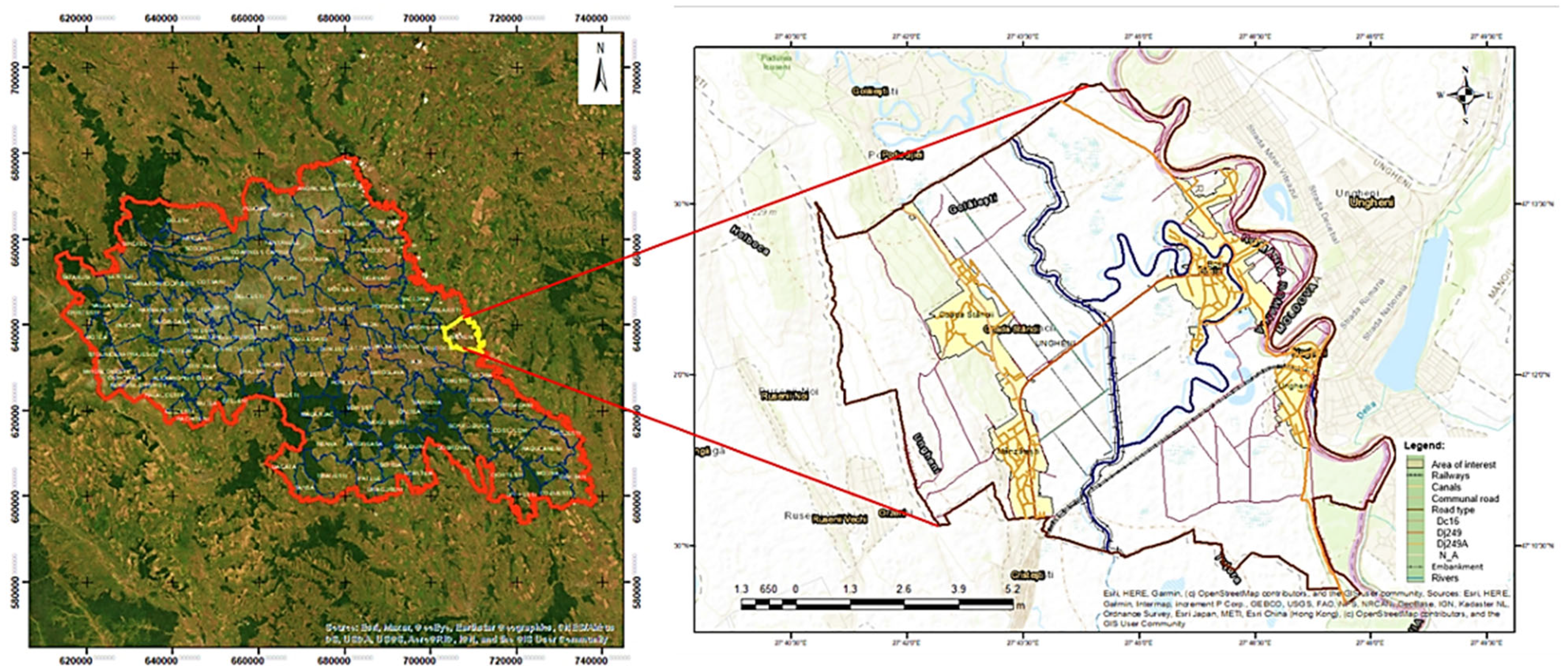
The study area is located in Ungheni, a locality situated in the eastern part of Iași county, at a distance of 21 km from the municipality of Iași (Romania), on the road from Iași to Chisinau (Figure 3). In the eastern part, the locality is bordered by the Prut River, which separates it from the town of Ungheni in the Republic of Moldova. It borders Golăești locality to the north, Țuțora locality to the south, the Republic of Moldova to the east, and Holboca locality to the west. The name originates from “unghi,” which means “angle” in Romanian, and refers to the fact that the town of Ungheni is situated at a bend in the Prut River [25]. It is also part of the Iași metropolitan area, where major infrastructure projects are being planned to connect the infrastructure networks of Romania and the Republic of Moldova, including the gas pipeline, the bridge over the Prut River, the A8 motorway, and other elements linking to the existing infrastructure. These investments will enhance the development of the area from all perspectives, including urban development, which requires an early assessment of risks, such as flooding, given the presence of two significant rivers in the area: the Prut River and the Jijia River. The flood risk on the Prut River has been modeled and evaluated according to EU Directive 2007/60/EC and is published online for public use/consultation (www.inundatii.ro) [47]. In this study, the flood hazard for the area surrounding the Jijia River is evaluated, optimizing the use of geospatial data by reusing and updating it from other new data sources.
The territory of the locality of Ungheni is located in the middle hydrographic basin of the Prut River. The Prut and Jijia rivers represent the hydrographic network. The Stânca regulates the hydrographic regime of the Prut-Costeşti reservoir in Iași County.

3.2. Input Datasets

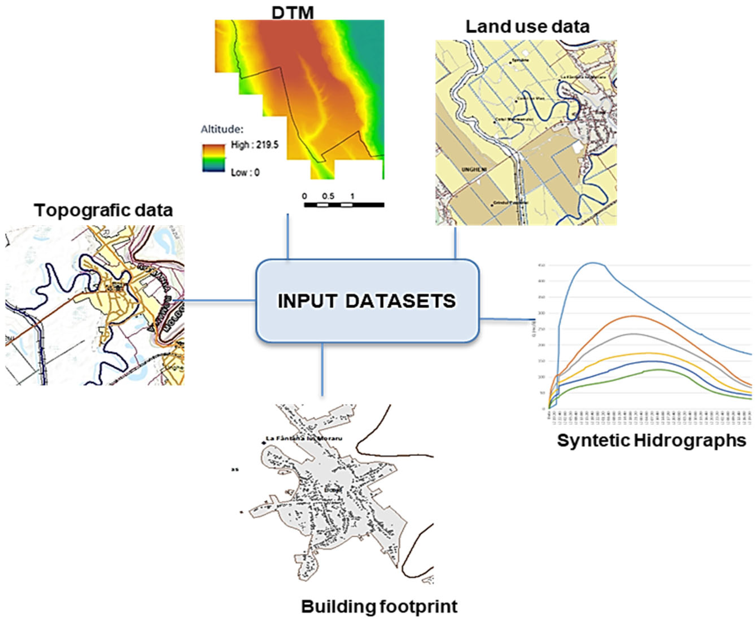
Geospatial layers were collected and processed to facilitate subsequent hydraulic modeling endeavors. The spatial resolution of the computational grid was reduced to optimize computation time and the use of available hardware resources. The choice of resolution does not compromise the model’s ability to reproduce the hydrodynamic processes of interest at the studied scale; rather, it represents a methodological compromise between the accuracy of the results and numerical feasibility [48]. In this study, we use the following data sources.
(1)
The main data source for deriving the DTM of the study area is represented by an Airborne Laser Scanning (ALS) dataset acquired in 2012 with the LEICA ALS 70 sensor and a wavelength of 1064 nm, for modeling flood hazard and risk maps in the Prut-Bârlad hydrographic basin according to European Directive 60/2007. These LiDAR data were reused in the present study and specifically processed to obtain the DTM on which the hydraulic model in HEC-RAS was based. The LiDAR strips have an average length of 45 km and a width between 1.5 km and 2.0 km, these specific dimensional parameters being required for precision reasons, taking into account the use of IMU inertial systems. The rectangular plane coordinates were calculated in the WGS84 Universal Transverse Mercator System zone 35N, and the altitudes in the WGS84 ellipsoidal reference system. The spatial resolution of the scan is 1 point/4 m2, and in the overlapping areas between strips, it reaches 1 point/2 m2. The use of airborne LiDAR technology in hydrological and hydraulic modeling is the best option since the altimetric precision is superior to the planimetric precision [49].
(2)
In this study, we also employed topographic data comprising the river network, road network, railways, and delineation of the study area, as well as defensive structures. We accurately delineated the last using vectorization techniques based on the high-resolution digital terrain model (1 × 1 m), with a vertical accuracy of 10 cm.
For computational efficiency, a variable 2D mesh was applied: 2 × 2 m cells for critical features (minor channels, roads, levees) and 8 × 8 m cells in less sensitive floodplain areas. This ensures accurate representation of narrow features while keeping computation times manageable.
(3)
The building footprint data are sourced from the National Cartography Center (CNC), under the coordination of the National Agency for Cadastre and Land Registration (ANCPI). These georeferenced vector datasets provide accurate building outlines within the study area and are regularly updated to reflect recent urban development. Their integration into hydraulic models enables realistic flood simulations in urban settings and improves flood risk assessments (Figure 4).
(4)
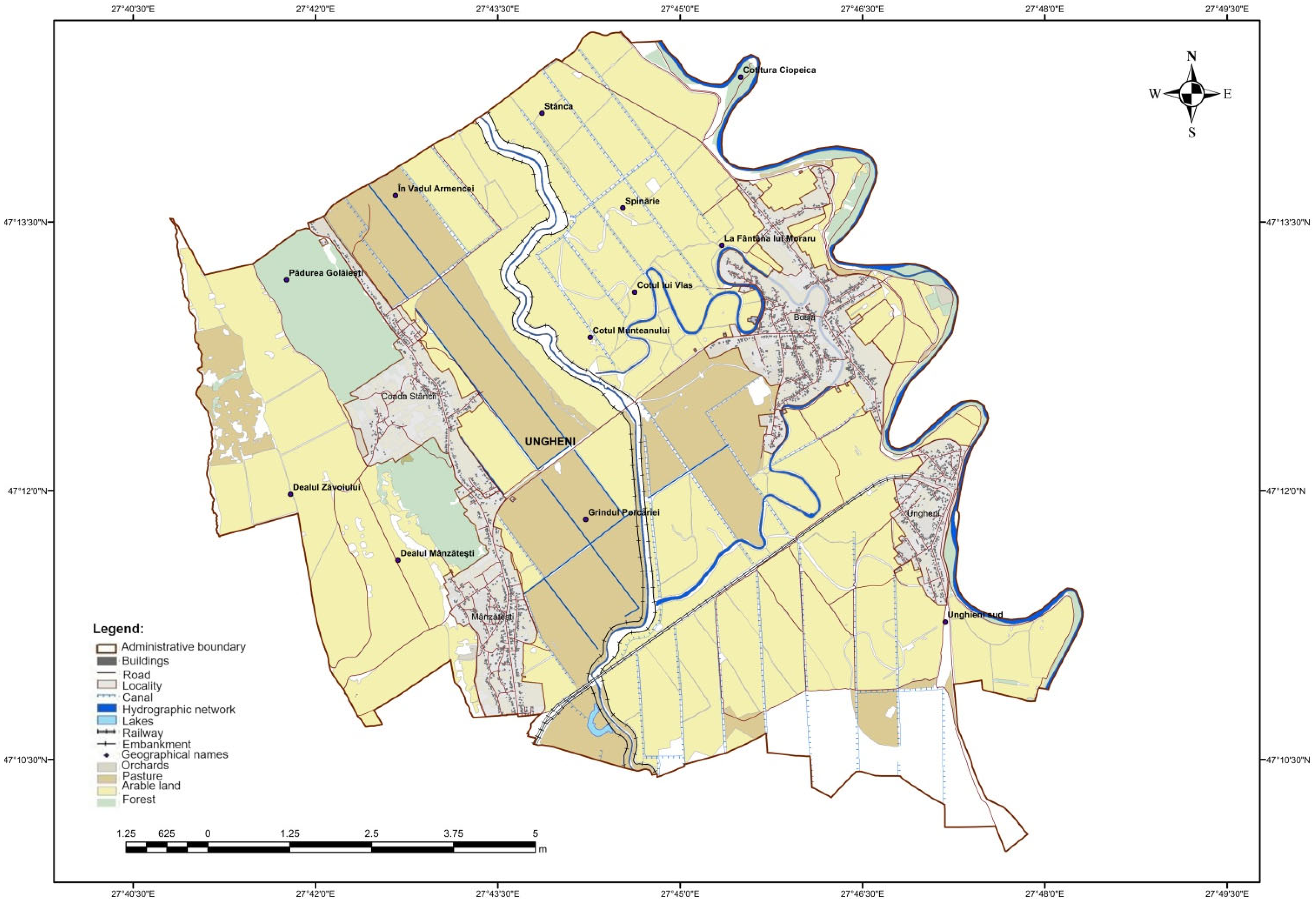
Land use data represent another important input dataset (see Figure 5). We derived these data from the 2020 color orthophoto plan provided by the National Agency for Cadastre and Land Registration (ANCPI), captured at a scale of 1:5000 and delivered in raster format with a spatial resolution of 50 cm. The data acquisition involved both analog and digital sensors, including the analog ZEISS LMK camera (model RC30) and digital sensors such as the Inertial Measurement Unit (IMU) and Digital Mapping Camera (DMC) with a focal length of 120 mm. Additional ancillary databases from APIA (Agency for Payments and Intervention in Agriculture) were used to support land use classification. These land use data were subsequently employed to estimate surface parameters relevant for hydraulic modeling, such as Manning’s roughness coefficients.
(5)
Another input dataset represented by the climatology data, including precipitation and temperature records, was provided by the national meteorological services to inform hydrological inputs and boundary conditions in the modeling process.

4. Proposed Methodology for Data Analysis

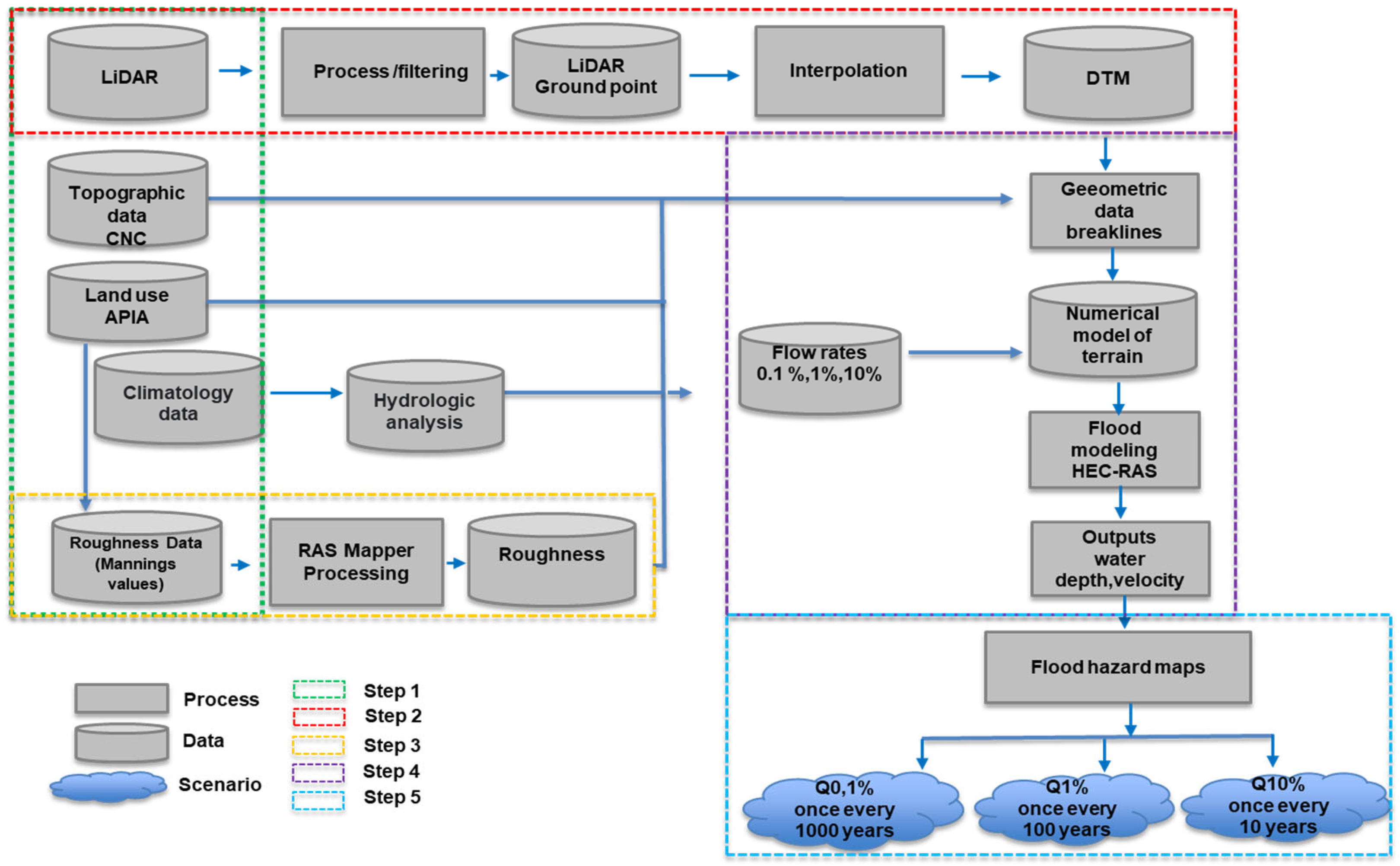
The proposed methodology is designed to guide the processing and interpretation of diverse datasets, enabling accurate hydrologic and hydraulic modeling. The workflow comprises several sequential stages, from data acquisition to the generation of actionable risk maps, ensuring data quality, consistency, and meaningful integration. Figure 6 illustrates the key steps involved in this methodology, highlighting the flow from raw input data to final outputs.
Workflow description
The proposed methodology to produce and analyze flood hazard maps consists of the following five main steps:
  • Step 1: Geospatial data preparation and pre-processing.
  • Step 2: Improved DTM derivation.
  • Step 3: Derivation of roughness layers.
  • Step 4: Hydraulic modeling.
  • Step 5: Hazard mapping.
Step 1: Preparation of geospatial data necessary for extracting the characteristic elements of the watershed (Figure 7). In Step 2 an improved DTM is derived by integrating buildings and infrastructure to accurately reflect physical obstacles. In Step 3, land use-based roughness layers are created, and Manning’s roughness coefficients (n) are assigned accordingly. In Step 4: Hydraulic modeling, the computational network is generated, boundary conditions are defined, and input hydrographs corresponding to Qp% exceedance flows are constructed, leading to Step 5, where flood hazard maps are generated through GIS-based integration of the model outputs.
Step 1: Geospatial data preparation and pre-processing
The flood risk analysis for the Jijia River Basin began with the collection and organization of relevant geospatial data. In this context, the geospatial data described in Section 3.2 were identified. Since these data were in different coordinate systems, WGS84 Universal Transverse Mercator (UTM) Zone 35N and Stereographic 1970 Krasovsky 1940 Pulkovo, it was necessary to convert them uniformly into the Stereographic 1970 coordinate system, the official coordinate system adopted in Romania, by employing the built-in transformation functions of ArcGIS Pro 3.1 software. These data formed the initial GIS database from which various geospatial elements specific to hydraulic modeling were extracted: hydrographic networks, drainage channels, railways, roads (both communal and county), buildings, agricultural and forested areas, as well as other areas of interest.
Step 2: DTM derivation
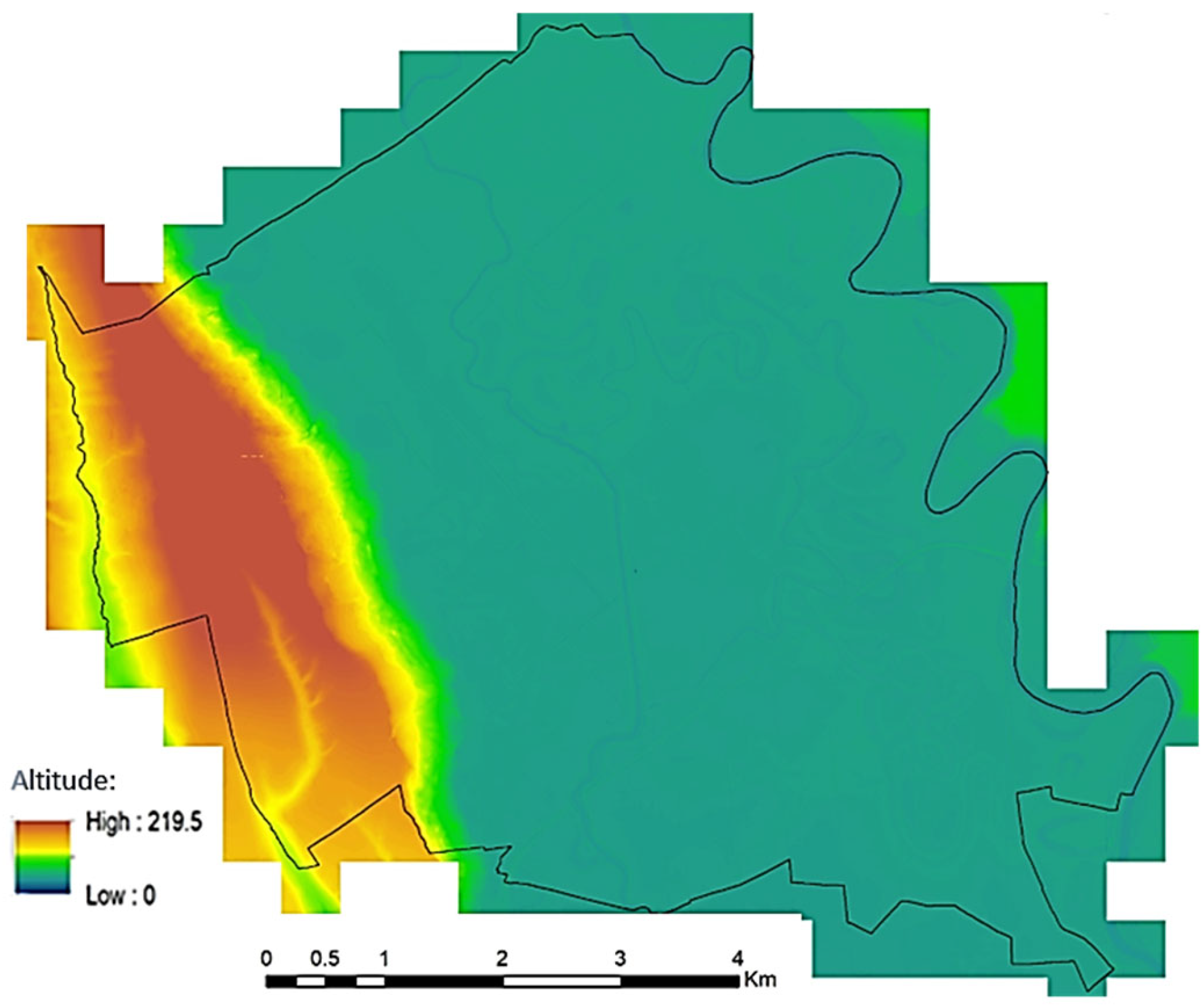
The DTM was derived from ALS data acquired with a LEICA ALS 70 sensor, providing an accuracy of 15 cm and 10 cm in the horizontal and vertical directions, respectively (according to the sensor specifications) using 9 strips described in Section 3.2 (Figure 8).
To obtain the DTM, it was necessary to process the LiDAR data by following several steps: automatic and manual processing, classification, and filtering. The automatic filtering was performed in Cloud Compare using the Cloth Simulation Filter (“CSF Filter”) algorithm, while the manual filtering was performed in ArcGIS Pro 3.1 software. After obtaining the ground points, converting the ellipsoidal height to Black Sea height was mandatory in order to produce a correct DTM that is compatible with other data sources. The ellipsoidal height transformation was performed through algebraic functions using the “raster calculator” functions in ArcGIS Pro 3.1 by employing the Romanian_ETRS89v102.gsf geoid model provided by ANCPI.
Step 3: Spatial variability of roughness coefficients
Accounting for spatial variability in surface roughness is a critical component in 2D hydraulic modeling, as roughness values can significantly influence flow behavior. However, this task poses notable challenges, since roughness varies depending on land use, vegetation cover, soil type, and local hydrodynamic conditions. These variations introduce uncertainty into the model calibration and may affect the reliability of flood predictions.
The estimation of Manning’s roughness coefficient n has been made from the following equation proposed in [49]:
n = A R 2 3 s 1 2 Q
where
  • Q represents the flow in cubic meters per second (m3/s).
  • A denotes the flooded area of the transversal section in square meters (m2).
  • R signifies the hydraulic radius of the transversal section, calculated as the ratio of A to the wet perimeter (R = A/P)—m2/m.
  • P is the wet perimeter of the transversal section—m.
  • s is the slope of the water surface—m/m.
  • n is Manning’s roughness coefficient—s/m1/3.
Manning’s n values were selected based on literature and adapted to local conditions: concrete channels (0.013–0.015), grass/vegetation (0.035–0.040), and urban areas with buildings (0.020–0.025). Sensitivity tests show that variations within these ranges have minimal impact on flood depths and extent.
Step 4: Hydraulic modeling
This step is the core of our approach and consists of identifying and defining the boundary conditions and generating the model itself. Our hydraulic model is implemented entirely in 2D using the HEC-RAS software. Boundary conditions include:
(a)
Upstream (i.e., describes the inflow characteristics at the upper limit of the hydraulic model domain derived from the INHGA synthetic hydrograph).
(b)
Downstream Normal Depth condition with a slope of 0.007, applied across the respective boundaries of the 2D domain (i.e., the outflow behavior at the lower end of the model domain).
(a)
Upstream condition:
In our study, the upstream condition was crucial in defining boundary conditions for hydraulic modeling. We employed synthetic hydrographs for various flow probabilities, including 20%, 10%, 5%, 2%, 1%, and 0.1% as suggested in [50,51].
In our study, the chosen percentages (e.g., 20%, 10%, 5%, 2%, 1%, 0.1%) refer to the exceedance probabilities associated with flow events, representing the statistical likelihood that a given flow rate will be equaled or exceeded within any given year. These exceedance probabilities are critical for flood risk assessment and hydraulic modeling as they characterize the frequency and magnitude of hydrological events. For instance, a 1% exceedance probability corresponds to a flow event with a 1 in 100 chance of occurring in any given year, often termed the 100-year flood event.
(b)
Downstream condition:
This refers to the slope of the terrain/downstream level of the river, which can be extracted directly from the RAS Mapper interface of the HEC-RAS software. A boundary condition is required at the downstream end of any river covered by the hydraulic model. These conditions are generally specified as water level hydrograph, flow hydrograph, rating curve at the hydrometric stations, normal depth, or critical depth limit condition [52].
Our model configuration involves the following processing steps: delimitation of the river catchment and the calculation range, generation of the calculation network, boundary conditions, construction of the input hydrograph corresponding to the flows with probability Qp% of exceedance, processing of the digital terrain model to level-up the constructions, and the generation of layers for roughness parameters.
For the downstream boundary condition, normal depth with a slope of 0.007 was applied, while the upstream inflow was defined using the INHGA synthetic flood hydrograph.
Generally, to solve the main flow directions, three to four cells of the computational grid (domain discretization) are required. This imposes a limitation on the minimum resolution usable for modeling 2D rivers and streams [52]. For instance, modeling a 5 m wide valley in 2D may require a minimum computational grid resolution of approximately 1.5 m, while for a 30 m wide river, a 10 m resolution might be sufficient [53].
We used a computational timestep of 10 s, determined through stability testing to satisfy the Courant–Friedrichs–Lewy (CFL) condition in the urban mesh. Hydrograph inputs were provided at 10 min intervals, and the Diffusion Wave equations were applied. Stability checks confirmed that the chosen timestep ensures numerical stability across the entire 2D domain.
Step 5: Flood hazard maps production
Flood hazard mapping is accomplished by overlaying and intersecting the water surface from the hydrodynamic modeling stage with the DTM in a GIS environment. This process allows the visualization and analysis of flood extents and hazard zones [54,55]. In the case of the present study, flood hazard bands with return periods of 0.1%, 1%, and 10% were generated in raster format, where the cell attributes are water velocity and depth. Based on these attributes, flood hazard bands were further generated in shapefile format. This new layer defining flood hazard was overlaid on the existing geospatial database, thus obtaining flood hazard maps. Through this process, a new geospatial database was generated, which is further used in the GIS environment, employing specific analysis tools for flood risk assessment.

5. Results and Discussion

5.1. Improved DTM Derivation

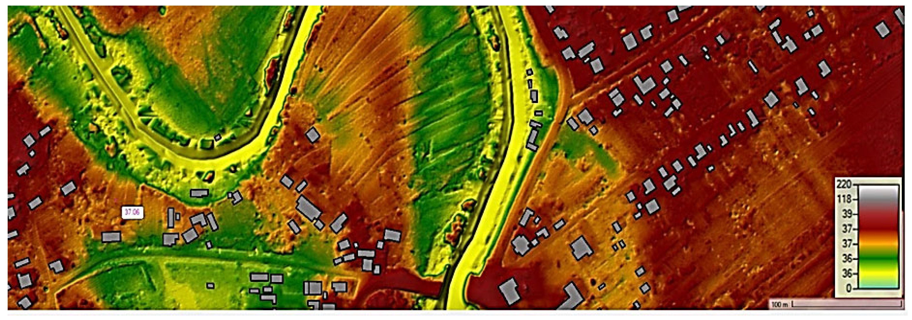
After the filtering process, the ALS ground point clouds were interpolated into 1 m spatial resolution DTM. The next step was to enhance the DTM realism and accuracy by incorporating key physical features. Building footprints are elevated to their threshold elevation to simulate their impact on flow obstruction (Figure 9). In addition, other critical elements, such as riverbanks, roads, railways, and flood defense structures, are integrated into the terrain model based on LiDAR data and vector layers. These features are either preserved or adjusted to reflect their real elevation and function, improving the accuracy of hydraulic simulations in both urban and peri-urban contexts, as emphasized in [56].

5.2. Roughness Coefficient Estimation

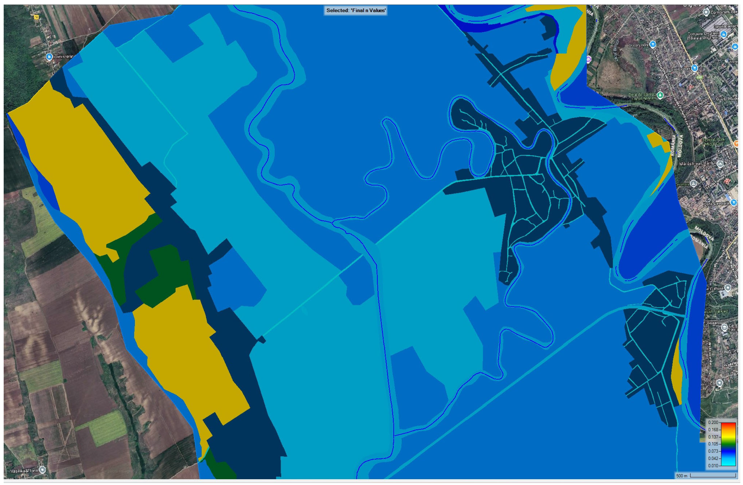
In two-dimensional hydraulic modeling, representing how surface resistance changes across space is essential because it strongly affects the movement of water. Yet, assigning appropriate resistance values is difficult, as they differ according to land cover types (Figure 10), vegetation density, soil properties, and site-specific flow conditions.
For the estimation of Manning’s roughness coefficient n, the model domain was subdivided into 10 distinct land use classes, and each class was assigned a Manning’s n coefficient based on its hydraulic characteristics. For instance, natural streambeds with vegetation and stones were assigned n = 0.04, arable land n = 0.05, asphalt roads n = 0.016, smooth concrete n = 0.09, dense forests n = 0.15, and short grass pasture n = 0.035. Other categories, such as unproductive land or areas with tall vegetation, received values between n = 0.07 and 0.10 (Table 1).
These coefficients were automatically attributed using a land use classification layer derived from the 2020 ANCPI orthophoto (at 1:5000 scale), supplemented with agricultural land data from APIA. The selection of n values was based on established hydrological literature [42] and international modeling guidelines, with adjustments made to reflect the specific characteristics of the local terrain. We chose this approach to ensure that the hydraulic model realistically simulates the spatial distribution of flow resistance, allowing water movement to interact differently with each surface type. This enhances the model’s sensitivity to terrain heterogeneity and improves the reliability of flood extent and depth estimations, particularly in mixed-use and peri-urban environments where land use can vary significantly over short distances.

5.3. Hydraulic Modeling Results

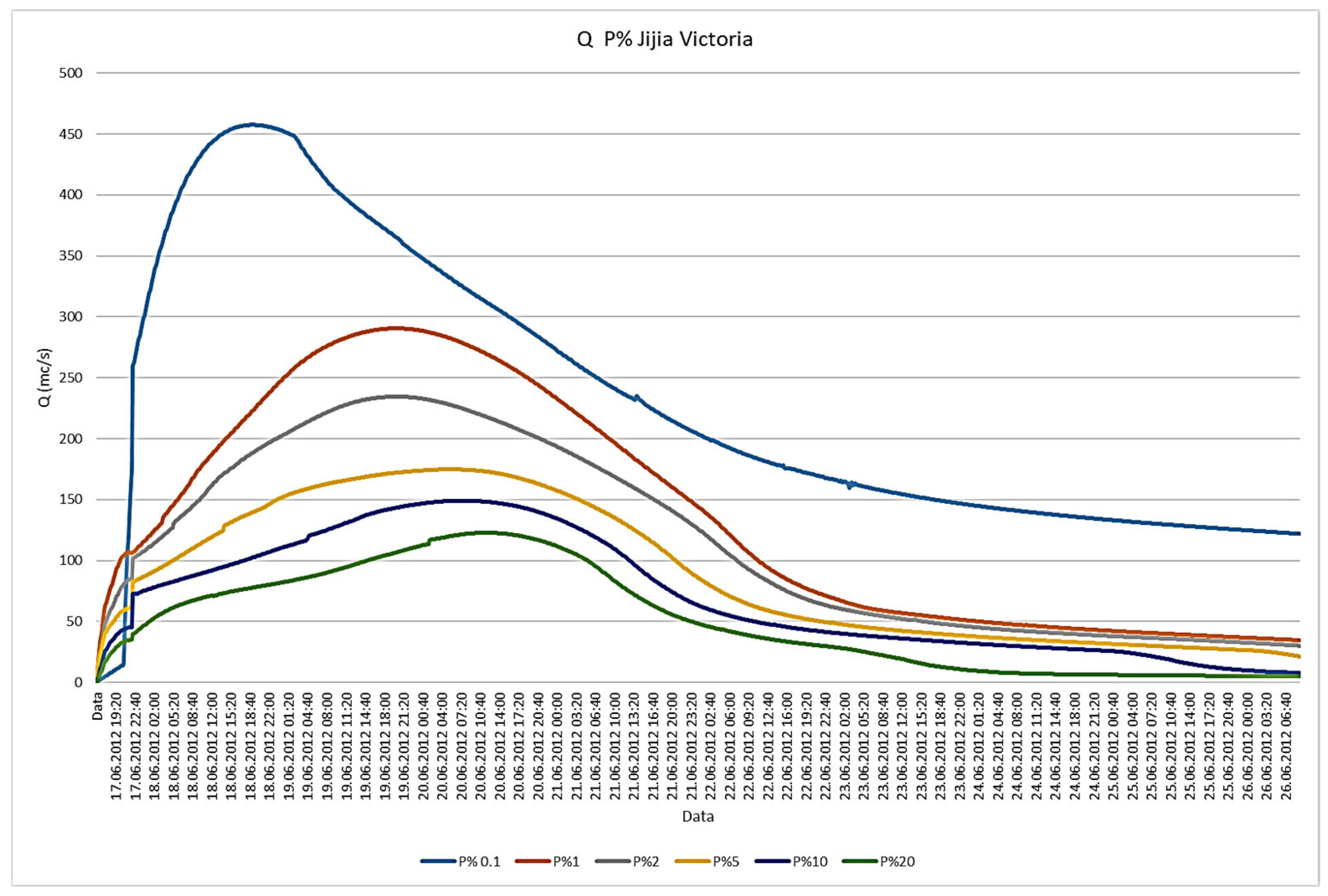
In our study, the employed synthetic hydrographs were provided by the Institute of Hydrology and Water Management, coming from the nearest upstream hydrometric station, specifically the Victoria hydrometric station situated on the Jijia River (see Figure 11 and Figure A1).
The synthetic hydrographs were employed as boundary conditions in the model to simulate river responses under varying flow scenarios, ranging from regular discharges to rare extreme flood events. Selecting a representative observed event for calibration requires careful consideration, typically involving time series data with a 10 min interval. To ensure accuracy and reliability, the hydrographs must be adjusted to match the estimated flow rates, which may involve altering parameters in the rainfall–runoff model or scaling the hydrograph shape accordingly [57].
In the present study, synthetic flood hydrographs with return periods of 0.1%, 1%, and 10% were selected and further used in the analysis, as they best characterize the flood hazard in the studied area.
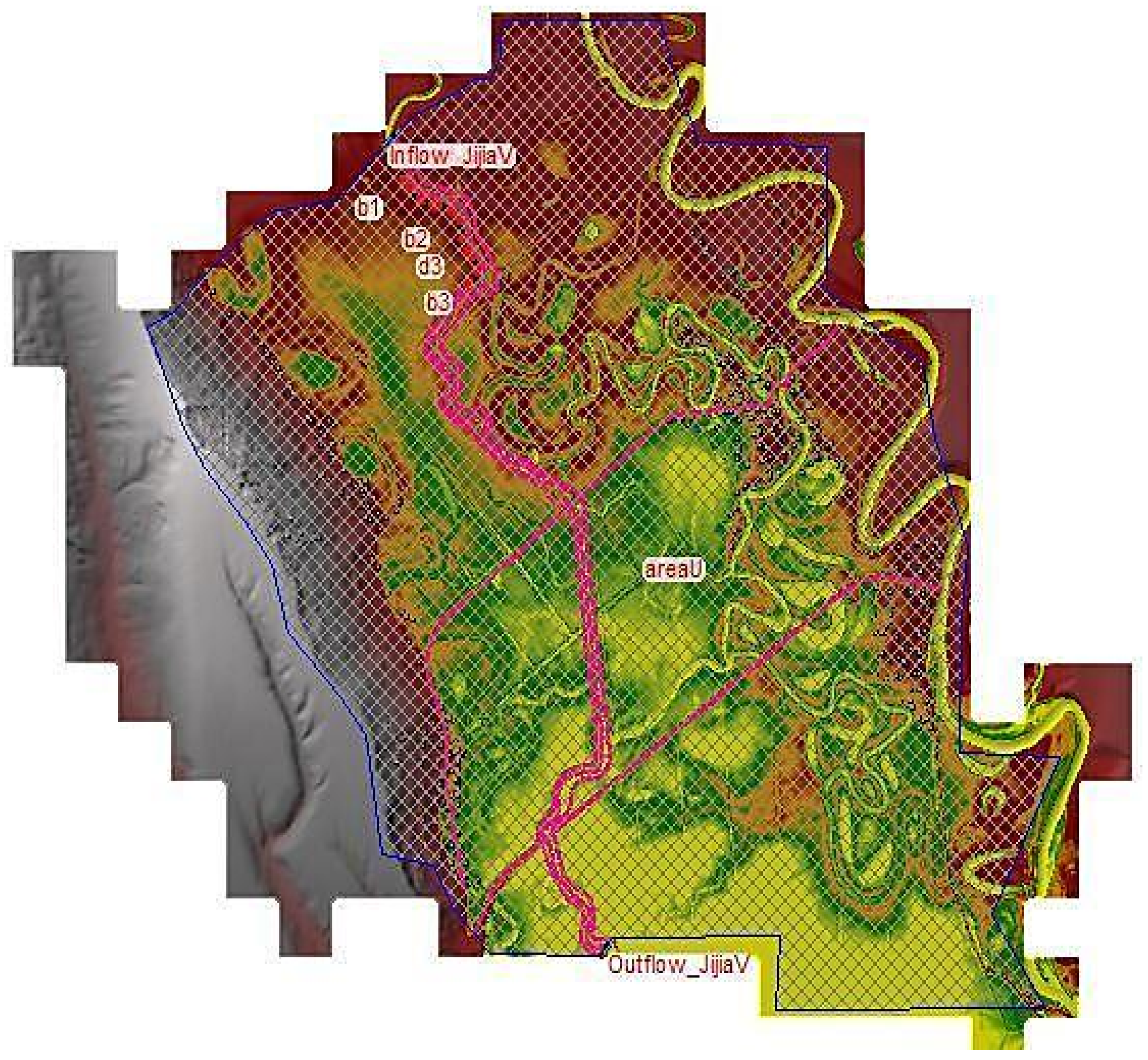
In scenarios where the simulated flows exceed the channel’s transit capacity, it is necessary to predefine the flood zones. This involves describing the riverbed and floodplain using a grid or raster domain, which is based on the DTM, to which geometric data is added in HEC-RAS. These geometric data refer to the definition of flow areas, including areas with inefficient flow as well as impermeable areas (dikes, bridges, constructions, etc.). In our case, in the study area, it was necessary to define the following geometric data: the hydrographic system cross-sections, the left and right bank levee, the areas with ineffective flow, the old course of the Jijia River, the embankment of DN 249A road, the bridge over the Jijia River related to the locality of Ungheni, and breaches in the levees related to the agricultural exploitation roads on the localities of Manzatesti and Coada Stancii.
2D modeling in HEC-RAS is a basic step in hydraulic analysis and involves the complete definition of the geometry of the analyzed river or channel (Figure 12). This is performed by integrating geospatial data from the relevant topographic layer into the DTM. In the Geometric Data module of HEC-RAS, these data become key parameters for simulating surface runoff and identifying flood-prone areas. The following elements were defined in the model geometry: the hydrographic system (schematic representation of the river section), hydraulic structures (bridges, footbridges, levees, breaches), and flow obstructions (such as buildings or islands). For the study area, a 2 × 2 and 8 × 8 m mesh cells were generated, into which all the breaklines previously defined in the geometry were incorporated. The 2 × 2 m resolution mesh was used for the minor riverbed (for critical features, including minor channels, roads, and levees), while the 8 × 8 m resolution mesh was used for the rest of the areas in the analyzed region (in floodplain areas, outside the main channels). The spatial resolution of the computational mesh was reduced to optimize computation time and the use of available hardware resources. The choice of resolution does not compromise the model’s ability to reproduce the hydrodynamic processes of interest at the studied scale; rather, it represents a methodological compromise between the accuracy of the results and numerical feasibility [48].
Exposure elements, such as buildings, are also taken into account in river modeling. A raising of the digital model of the land is made based on the footprint of the buildings (Figure 13).
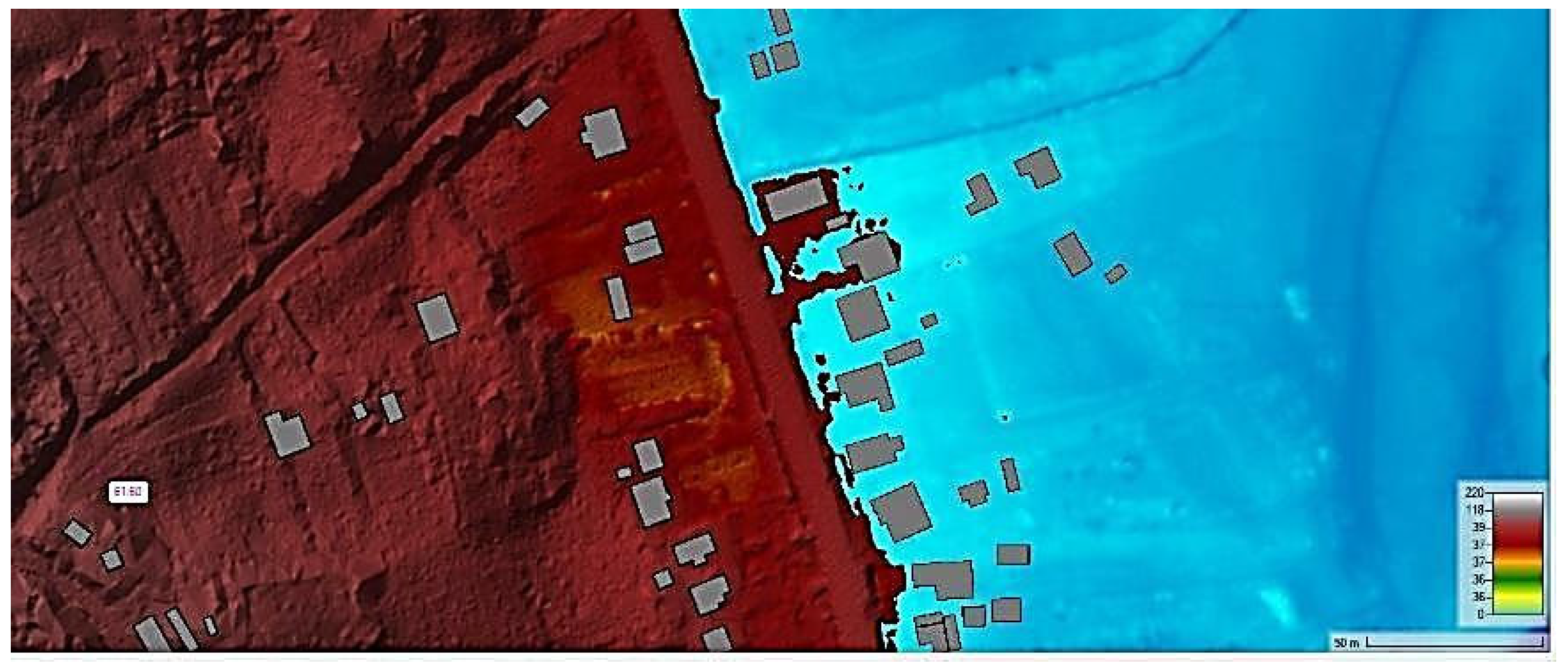
The footprint of the buildings serves as an important layer in 2D type modeling, allowing us to accurately determine if they lie within the flood zone or are shielded from potential floods (see Figure 14).
In the process of hydrological and hydrodynamic modeling, accurate information regarding land use is indispensable. Flood waves simulated for different probabilities of exceedance can be significantly influenced by land use, impacting the flow route and overflow limits. Integrating the land use layer into the hydraulic model allowed us to assess how different soil cover types influence flood wave propagation. Urban areas promoted faster flow, agricultural lands and pastures partially slowed the runoff, while forests significantly reduced flow velocity. This spatial variation in Manning’s roughness coefficient directly impacted the extent of simulated flood-prone areas in the Ungheni locality. This information was acquired through photo interpretation from orthophoto maps or through direct observations.

5.4. Model Calibration and Scenario Predictions

In this study, we employed synthetic hydrographs supplied by INHGA, which had been pre-calibrated using historical flood records. The calibration process consisted of resampling the hydrographs to 10 min intervals and analyzing probabilistic flow distributions to delineate the main channel and validate the floodplain extent. Owing to the absence of upstream hydrometric stations for the 2012 flood event, conventional performance indicators such as NSE, RMSE, or Bias could not be computed. This methodological choice is consistent with established practices in data-scarce settings. Although direct observational validation was not feasible, the outcomes are in line with high-resolution urban flood mapping efforts reported in Europe and demonstrate a transferable workflow for flood hazard assessment under conditions of limited hydrological information.
In the model calibration process, determining scenarios and running the model are key steps. Achieving accuracy in predicting the maximum river level depends on the time duration of the hydrograph. Typically, a deviation of up to 30 min from the actual occurrence time is considered acceptable in many cases. However, river basins characterized by a longer growth time may warrant a higher tolerance threshold. Conversely, for basins with a rapid response, a tolerance as low as 15 min may be necessary to ensure accurate predictions. In the present study, considering that the time step of the synthetic input hydrograph was 10 min, all output data were calculated at the same 10 min interval (Figure 15).

5.5. Extraction of Results: Types, Generation, Storage, and Processing

In the extraction of results, various types of data are generated, stored, and processed to provide valuable insights (Table 2).
The two-dimensional (2D) hydraulic simulations conducted with HEC-RAS produced eight primary types of outputs, extracted and processed using ArcGIS Pro, employing the Raster to Polygon function to convert flood depth rasters into vector polygons, and organized by each scenario accordingly (10%, 1%, 0.1% exceedance probability). The use of high-resolution LiDAR-derived DTM (1 m) allowed for accurate flood modeling in both urban and rural contexts.
Maximum water depth was generated as raster files, indicating inundation severity. Areas with depths below 0.1 m were filtered out. The <0.1 m threshold is used solely for visualization purposes in the map legend and does not affect the underlying simulation data. All shallow flows, including those around buildings, are fully retained in the model computations. These resulting layers were later used for classifying flood intensity and for exposure analysis.
Flow velocity rasters were extracted per scenario to assess the energy of floodwaters. These helped in identifying areas with high erosive or structural impact potential.
Flood extents were derived from depth rasters and stored as vector polygons. These delineate the spatial spread of each simulated flood scenario and serve as the basis for intersection with exposure layers.
Hazard level maps (depth × velocity) were computed and classified into low, moderate, and high hazard zones. These were used to inform priority areas for intervention.
Building exposure was assessed by intersecting flood extents with ANCPI building footprints. Under the 0.1% scenario, 882 buildings (totaling 62,600 m2) were affected, primarily in Coada Stâncii and Mânzătești.
Affected land parcels were identified using cadastral data. For example, the 1% scenario impacted 18 land plots (~152 ha), while the 0.1% scenario affected 42 plots totaling over 840 ha.
Exposed infrastructure, including roads and railways, was quantified by intersecting linear networks with flood extents. In the 0.1% case, 55 segments were exposed, totaling 13.5 km.
Final flood hazard maps were created for each scenario and exported as both raster layers and printable PDFs. These maps, shown in Figure 16, visualize depth, velocity, and affected assets.
Note that ArcGIS serves as a versatile tool for extracting different geospatial data, enabling the extraction of speed and water depth files; nevertheless, the study can be reproduced in other open-source GIS tools such as QGIS. These files contain detailed information stored in raster format, with each cell representing different values of depth at a resolution of 2 × 2 m. This pixel resolution ensures accuracy and granularity in the analysis of hydraulic modeling results, as proved by [58,59].
The 2D hydraulic simulations performed with HEC-RAS yielded eight primary output types, systematically extracted and processed within ArcGIS Pro, and organized according to three flood scenarios corresponding to 10%, 1%, and 0.1% exceedance probabilities. Utilizing a high-resolution LiDAR-derived DTM at 1 m resolution enabled precise flood modeling across both urban and rural landscapes.
According to the data presented in Figure 16, the study analyzes three flood risk scenarios based on annual exceedance probabilities of 10%, 1%, and 0.1%. These probabilities correspond to flood events with different recurrence intervals:
(a)
10%—frequent floods, likely to occur approximately once every 10 years;
(b)
1%—moderate floods, with a recurrence interval of about 100 years;
(c)
0.1%—rare floods, expected to occur once in 1000 years.
To better understand the impact of these scenarios on local infrastructure, we used geospatial databases corresponding to each probability level.
In the case of the least likely scenario (0.1% probability, Figure 16c), the affected areas include the villages of Coada Stâncii and Mânzătești. Here, flood events could impact 882 buildings, covering a total footprint of over 62,600 square meters, 42 land parcels of various use categories totaling more than 840 hectares, and 55 infrastructure segments with a combined length of 13.5 km.
Under the moderate-risk scenario (1% probability, Figure 16b), the exposed area includes the village of Ungheni. In this location, flood risk may affect two small buildings (with a total footprint of 4.5 m2), 18 land parcels with diverse functions amounting to nearly 152 hectares, and three road segments totaling 710 m in length.
As for the high-probability scenario (10%, Figure 16a), no significant damage is anticipated.
Due to factors such as intensive land use, inadequate or aging infrastructure, and local topographic features that concentrate or slow water flow, certain areas are more vulnerable to flooding than others. While the current flood extents are modeled deterministically, this approach cannot capture the full range of possible outcomes or the inherent variability in flood behavior. Incorporating uncertainty visualization, such as probabilistic flood maps, would improve risk assessment and support more informed decision-making for planners, communities, and policymakers.
Considering the increasing frequency and intensity of flood events driven by climate change, the presented flood modeling framework offers a robust tool for anticipating future flood risks and supporting adaptive planning and mitigation efforts.

6. Discussion

Our proposed workflow and obtained results align well with international best practices in utilizing GIS and 2D HEC-RAS modeling but distinguish themselves by focusing on multi-metric vulnerability analysis and data-transferable workflows in contexts typically constrained by data availability (Table 3). Specifically, the use of LiDAR-derived DEMs, GIS integration, and 2D HEC-RAS multi-scenario modeling (including the explicit incorporation of anthropogenic features and synthetic hydrographs) for improved accuracy and efficiency mirrors high-fidelity approaches used in Romania [26,30], Turkey [28], and other urban studies [30,31,36,41]. However, our contribution to integrate the full spectrum of 2D hydrodynamic outputs (depth, velocity, arrival time, duration, and recession time) for multivariate vulnerability assessment sets it apart from typical international studies that often focus mainly on flood extent and water depth, and directly addresses the identified critical omission in the field [26,36]. Furthermore, the proposed methodology of utilizing certified synthetic hydrographs to reduce the need for lengthy hydrological simulations offers a practical, transferable solution for flood hazard mapping in data-scarce regions, contrasting with the challenges faced in traditional coupled HEC-HMS/HEC-RAS studies [28,31] or those reliant on high-volume observation data (“Big Data”) for validation [31].
The current scientific landscape in flood risk management presents a significant knowledge deficiency stemming from the slow progress in adopting holistic, resilience-focused systems and the persistent failure to conduct integrated multivariate vulnerability assessments [34]. While 2D hydrodynamic models can generate a full spectrum of data, previous studies suffer from the critical omission of comprehensively analyzing time-variant flood characteristics—specifically flood velocity, arrival time, duration, and recession time—which are essential inputs for detailed disaster mitigation and evacuation strategies [36]. This methodological challenge is exacerbated by unresolved technical imperatives related to input data and computational efficiency: achieving high-fidelity urban simulations requires leveraging high-resolution geospatial inputs like LiDAR-derived DEMs while explicitly integrating anthropogenic features to accurately capture local flow dynamics; simultaneously, regions with limited hydrological input data require the validation of transferable workflows that utilize certified synthetic hydrographs to replace lengthy hydrological simulations. Finally, the computational cost of high-resolution 2D modeling introduces an operational deficit that necessitates determining the optimal mesh grid size threshold to balance required accuracy with minimizing simulation runtime, thereby managing the “Big Data” generated by these complex simulations for timely decision support [31].
Compared to previous studies, the main contribution of this flood modeling approach lies in the integration of advanced 2D hydraulic modeling (using HEC-RAS 2D) with high-resolution spatial data. This includes a 2 × 2 and 8 × 8 m DTM generated from LiDAR data and detailed building footprints, which help to accurately represent flow obstructions. The model also uses a hybrid mesh system that adjusts resolution based on the complexity of the terrain, allowing for greater detail where it matters most. Additionally, synthetic hydrographs for different exceedance probabilities are incorporated directly into the model, avoiding the need for time-consuming hydrological simulations. Together, these elements provide a more realistic, efficient, and practical way to simulate flood dynamics, especially in densely built urban areas.
In some cases, higher-resolution DTM data may be necessary to identify preferential flow paths and major riverbed blockages. Detailed flood studies at the local level require more precise DTM data compared to broader strategic or basin-level studies. Recommendations suggest a vertical accuracy of 0.5 m and a spatial resolution of at least 10 m for major rural riverbeds. Conversely, urban areas may require a vertical accuracy of 0.05 m and a spatial resolution of 0.5 m to account for the finer details, such as distances between buildings.
Although the results of this study are specific to the Ungheni area, the modeling approach, combining HEC-RAS and GIS, is flexible and can be applied to other regions, as well. However, adjustments are needed based on local data such as terrain, land use, and hydrological characteristics. The model is not one-size-fits-all, but it provides a transferable framework that, with proper calibration, can support flood risk assessments in different contexts.
One of the limitations of our approach is related to the temporal mismatch between the different datasets: while land use and building footprint data are based on 2020 orthophotos and official updates, the DTM originates from 2012 LiDAR strips. Despite this 8-year gap, the main flow corridors and floodplain geometry remain stable at the catchment scale. Minor local changes (e.g., new structures or grading) may slightly affect flow paths, representing a source of uncertainty that can be addressed once a more recent DTM becomes available.
Although our model produced depth × velocity maps, a standardized threshold-based hazard classification was not applied. The main reason for this consists of the fact that the primary focus falls on assessing the direct exposure of critical infrastructure to flooding by analyzing the extent of inundated areas. Since the study is primarily aimed at practical utility for local urban planning, mapping flood extent was more relevant than differentiating hazard intensity levels. However, we acknowledge that the absence of classification thresholds limits the comparability of our results with other international studies. For this reason, in future work, we intend to test established classification schemes (e.g., EU Floods Directive, UK DEFRA guidelines) in order to enhance reproducibility and allow our results to be more easily integrated into a broader comparative framework.
Future research in urban flood modeling could focus on integrating artificial intelligence, real-time data, and multi-hazard approaches. AI techniques can enhance flood prediction, calibration, and hazard mapping, while real-time sensor and UAV data allow dynamic model updates for rapid forecasting. Considering compound hazards, such as floods combined with landslides or extreme rainfall, can provide a more comprehensive risk assessment, supporting effective planning and mitigation strategies.
Future research in advanced flood modeling strongly mandates the expanded integration of AI/ML for computational optimization and dynamic forecasting, real-time data assimilation for enhanced situational awareness, and the adoption of broader multi-hazard and systemic management frameworks. Specifically, the focus should be on developing AI-driven surrogate models (like Next-Gen GMDH, ELM, and DNN architectures) to replace computationally expensive hydrodynamic simulations (HEC-RAS 2D/HEC-HMS), achieving near-real-time flood forecasting by predicting flood depth, velocity, and recession much faster than traditional methods [60,61,62,63]. Simultaneously, this predictive capability must be fueled by real-time data assimilation using various sensors, including smart city video surveillance and computer vision (YOLO, DETR) for monitoring flood extent and depth, alongside the integration of Volunteered Geographic Information (VGI) to supplement traditional measurements and provide prompt awareness [62,64]. Finally, the field must advance towards multi-hazard and systemic risk management by exploring how Large Artificial Intelligence Models (LLMs) can integrate heterogeneous data (textual, GIS, satellite imagery) to improve flood knowledge and risk perception [62], while expanding predictive modeling to capture cascading failures across interdependent infrastructure networks (like roads and power grids) caused by flood events [63,64].
Integrating hydrodynamic modeling (such as HEC-RAS), advanced machine learning (ML) algorithms, and high-resolution remote sensing (RS) data provides a robust and comprehensive framework for urban flood risk assessment and susceptibility mapping (Table 4) [51,65,66,67,68,69]. Specifically, hydrodynamic models like HEC-RAS are used to simulate flood dynamics and generate spatial inundation extents (often for large return periods like 100-year events), creating the necessary flood inventory and targets, which are then fused with geospatial and topographical input factors derived from remote sensing data (e.g., Lidar, DEMs, satellite imagery) to train and validate ensemble ML models. This combined methodology enhances predictive accuracy and computational efficiency, overcoming the limitations of using these techniques in isolation, and ultimately provides planners and policymakers with effective tools for targeted flood mitigation strategies and resilient infrastructure design [51,68,69].

7. Conclusions

This study applied a high-resolution flood modeling framework that integrates 2D hydraulic simulations in HEC-RAS with geospatial analysis to evaluate flood risk for exceedance probabilities of 10%, 1%, and 0.1%. The results demonstrated that, under the rarest scenario (0.1%), 882 buildings with a total footprint exceeding 62,600 m2, 42 land parcels (~840 ha), and 55 infrastructure segments (13.5 km) are exposed to inundation, mainly in Coada Stâncii and Mânzătești. In contrast, the 1% scenario indicated more limited impacts, affecting 18 parcels (~152 ha), two small buildings, and 710 m of road in Ungheni, while the 10% scenario showed no significant damages. These findings highlight the spatial variability of flood risk and the particular vulnerability of low-lying settlements in the study area.
Beyond its compliance with EU Directive 2007/60/EC, the proposed modeling framework has direct implications for local flood risk management and urban decision-making. The high-resolution flood hazard maps generated in this study can be used by local authorities to identify vulnerable areas, prioritize protective infrastructure, and optimize land use planning in flood-prone zones. Moreover, the results provide valuable input for emergency preparedness strategies, such as evacuation routes and risk communication with residents. By integrating detailed hydraulic simulations with geospatial analysis, the methodology delivers actionable information that supports both strategic planning and day-to-day decision-making for sustainable urban development.
Considering the obtained flood risk results with return probabilities of 1% and 0.1%, as well as the importance and development prospects of the studied area, hydrotechnical arrangements may be considered in the area to mitigate or eliminate the hydrological risk, thus ensuring sustainable development in the strategic border area of the two states, Romania and the Republic of Moldova.
Future research should focus on extending the proposed methodology to other river basins to test its reproducibility and adaptability under various hydrological conditions. Incorporating unsteady flow scenarios and employing two or three-dimensional hydraulic modeling would allow for a deeper and more nuanced understanding of flood dynamics. Long-term projections that consider the influence of climate change on the hydrological regime contribute to a more accurate anticipation of future flood risks. Moreover, recent technological advances, such as high-resolution satellite imagery and artificial intelligence, open new opportunities to enhance the precision of floodplain analysis and mapping.
Assessing the current state of protective infrastructure and exploring alternative risk reduction strategies, such as expanding buffer zones or restoring natural wetlands, are important steps toward improving flood risk management. Addressing this issue from a multidisciplinary perspective, including ecological, economic, and social aspects, is important for developing sustainable and resilient solutions capable of reducing vulnerability for both human communities and ecosystems.
Directive 2007/60/EC recommends re-evaluating flood risk every six years; however, in the context of accelerated climate change, this frequency is most likely no longer sufficient. In this regard, we propose for the future to perform hydraulic modeling in HEC-RAS using the geospatial model developed in this study, coupled with an HBV hydrological model. The HBV-HEC-RAS model will use meteorological and hydrological data as input. The modeling will be triggered after a statistical analysis of the rainfall data recorded at the IAȘI meteorological station, the closest to our study area. In this way, the flood risk reassessment will be triggered as soon as a new historical maximum precipitation intensity is recorded. This approach will allow for a preventive assessment of flood risk in the context of the increasingly evident impacts of climate change and a re-evaluation of the timeframe (revising policy cadence) within which these assessments need to be carried out.
Finally, combining flood modeling with an assessment of existing protective infrastructure, buffer zones, and natural flood retention measures would contribute to a multidisciplinary approach that incorporates ecological, social, and economic perspectives. Such an approach is essential for developing resilient strategies that minimize both human and environmental vulnerability in the face of increasing flood hazards.

Author Contributions

Conceptualization, L.M.C., C.I.P., M.D. and A.-M.O.-R.; methodology, L.M.C. and C.I.P.; software, C.I.P.; validation, C.I.P. and L.M.C.; formal analysis, C.I.P. and L.M.C.; investigation, L.M.C., C.I.P. and M.D.; resources, L.M.C., C.I.P. and M.D.; data curation, L.M.C., C.I.P. and M.D.; writing—original draft preparation, L.M.C., C.I.P., M.D. and A.-M.L.; writing—review and editing, L.M.C., C.I.P., M.D., A.-M.O.-R. and A.-M.L.; visualization, L.M.C. and C.I.P.; supervision, C.I.P.; project administration, L.M.C.; funding acquisition, L.M.C. All authors have read and agreed to the published version of the manuscript.

Funding

This research was funded by the Joint Operational Program Romania-Republic of Moldova, grant number 2SOFT/4.2.77/2020, and the APC was funded by the authors.

Data Availability Statement

All data generated or analyzed in this study are available from the corresponding author on request.

Conflicts of Interest

The authors declare no conflicts of interest.

Abbreviations

The following abbreviations are used in this manuscript:
DTMDigital Terrain Model
LiDARLight Detection and Ranging
GISGeographic Information System
HEC-RASHydrologic Engineering Center’s River Analysis System
HEC-HMSHydrologic Engineering Center’s Hydrologic Modeling System
APIAAgency for Payments and Intervention in Agriculture
ANCPINational Agency for Cadastre and Land Registration (Romania)
CNCNational Cartography Center (Romania)
ALSAirborne Laser Scanning
IMUInertial Measurement Unit
DMCDigital Mapping Camera
UTMUniversal Transverse Mercator
EUEuropean Union
USGSUnited States Geological Survey

Appendix A

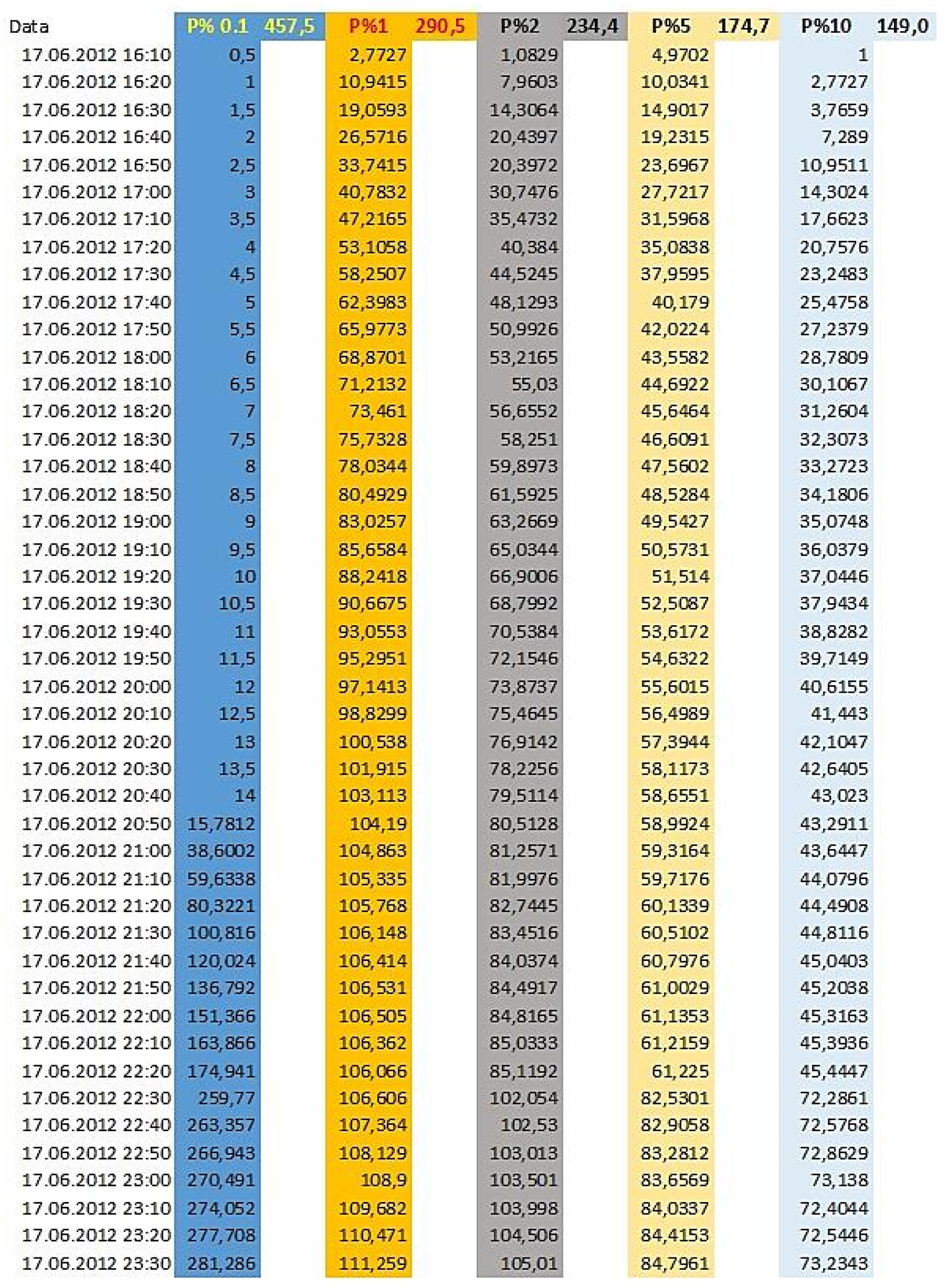
Figure A1. Input hydrographs corresponding to flow rates between 18 and 26 June 2012 with a probability of 20%, 10%, 5%, 2%, 1%, 0.1%.
Water 17 02959 g0a1

References

  1. Kundzewicz, Z.W.; Kanae, S.; Seneviratne, S.I.; Handmer, J.; Nicholls, N.; Peduzzi, P.; Mechler, R.; Bouwer, L.M.; Arnell, N.; Mach, K.; et al. Flood risk and climate change: Global and regional perspectives. Hydrol. Sci. J. 2014, 59, 1–28. [Google Scholar] [CrossRef]
  2. Oniga, V.E.; Crenganiş, L.; Diac, M.; Chirilă, C. Overview on Remote Sensing Methods and Data Sources for Floods and Landslides Management. Bul. Institutului Politeh. Din lasi. Sect. Constr. Arhit. 2020, 66, 59–70. [Google Scholar]
  3. Rentschler, J.; Salhab, M.; Jafino, B.A. Flood exposure and poverty in 188 countries. Nat. Commun. 2022, 13, 3527. [Google Scholar] [CrossRef] [PubMed]
  4. Brakenridge, G.R.; Anderson, E. Flood detection and monitoring using satellite data. In Remote Sensing of Floods; Springer: Dordrecht, The Netherlands, 2006; pp. 29–50. [Google Scholar]
  5. Anderson, R. Application of GIS in Hydrological Modeling. J. Hydrol. 2017, 123, 567–580. [Google Scholar]
  6. Demir, V.; Kisi, O. Flood Hazard Mapping by Using Geographic Information System and Hydraulic Model: Mert River, Samsun, Turkey. Adv. Meteorol. 2016, 4891015. [Google Scholar] [CrossRef]
  7. Almeida, G.A.; Silva, R.M.; Santos, M.J.; Costa, A.M. Hydrodynamic Modeling for Flood Risk Mapping Using HEC-RAS: A Case Study from a Semi-Arid Basin in Brazil. Water 2021, 13, 522. [Google Scholar] [CrossRef]
  8. Edirisooriya, E.M.N.T.; Neluwala, N.G.P.B.; Weerakoon, W.M.S.B. Flood Inundation Modelling in Greater Colombo Region Using HEC-RAS 2D. Eng. J. Inst. Eng. Sri Lanka 2022, 55, 21. [Google Scholar] [CrossRef]
  9. Adhikari, S. Evaluation of Model Parameter Sensitivity of Hec-Ras-2D Model on Flood Inundation Mapping Case Study of Surahi River and Banganga River, Nepal. Master’s Thesis, Institute of Engineering, Lalitpur, Nepal, 2020. [Google Scholar]
  10. Dottori, F.; Salamon, P.; Bianchi, A.; Alfieri, L.; Hirpa, F.A.; Feyen, L. Development and Evaluation of a Framework for Global Flood Hazard Mapping. Adv. Water Resour. 2018, 94, 87–102. [Google Scholar] [CrossRef]
  11. Di Baldassarre, G.; Schumann, G.; Bates, P.D.; Freer, J.E.; Beven, K.J.; Simpson, M. Floodplain Mapping: A Critical Discussion of Deterministic and Probabilistic Approaches. Hydrol. Process. 2010, 24, 1914–1924. [Google Scholar] [CrossRef]
  12. Ghimpu, L.; Apostol, L.; Rizea, I. Flood Hazard Mapping: A Case Study for Compliance with the European Floods Directive. J. Hydrol. Hydromech. 2019, 67, 175–185. [Google Scholar] [CrossRef]
  13. Neal, J.C.; Schumann, G.; Bates, P.D. A subgrid channel model for simulating river hydraulics and floodplain inundation over large and data-sparse areas. Water Resour. Res. 2012, 48. [Google Scholar] [CrossRef]
  14. Topolniceanu, A.; Balan, I.; Pricop, C.; Balan, I.E.; Giurma-Handley, C.; Crenganis, L. Runoff Simulation Through the Non-Permanent Accumulation Ciurea Using Hec-Ras 2d. Pangeea 2023, 14–22. [Google Scholar]
  15. US Army Corps of Engineers. HEC-RAS 2D User’s Manual. 2022. Available online: https://www.hec.usace.army.mil/software/hec-ras/download.aspx (accessed on 20 August 2025).
  16. Jha, A.K.; Bloch, R.; Lamond, J. Cities and Flooding: A Guide to Integrated Urban Flood Risk Management for the 21st Century; The World Bank: Washington, DC, USA, 2012; Available online: https://www.researchgate.net/publication/277827291_Cities_and_Flooding_A_Guide_to_Integrated_Urban_Flood_Risk_Management_for_the_21st_Century (accessed on 20 August 2025).
  17. Merz, B.; Kreibich, H.; Schwarze, R.; Thieken, A. Assessment of economic flood damage. Nat. Hazards Earth Syst. Sci. 2010, 10, 1697–1724. [Google Scholar] [CrossRef]
  18. Hagos, E.Y.; Gebremichael, M. GIS-based flood modeling and risk assessment using HEC-RAS: A case study of Awash River Basin, Ethiopia. Sustainability 2020, 12, 8082. [Google Scholar] [CrossRef]
  19. Horita, F.E.A.; de Albuquerque, J.P.; Marchezini, V.; Mendiondo, E.M. Bridging the gap between decision-making and hydrological modeling: A systematic review of flood risk decision support systems. Environ. Model. Softw. 2020, 129, 104697. [Google Scholar] [CrossRef]
  20. Alfieri, L.; Bisselink, B.; Dottori, F.; Hirabayashi, Y.; Naumann, G.; Salamon, P.; Sylla, M.; Feyen, L. Flood Risk Assessment at the Global Scale: A Review. Earth-Sci. Rev. 2020, 201, 102949. [Google Scholar] [CrossRef]
  21. Teng, J.; Jakeman, A.J.; Vaze, J.; Croke, B.F.; Dutta, D.; Kim, S. Flood inundation modelling: A review of methods, recent advances and uncertainty analysis. Environ. Model. Softw. 2017, 90, 201–216. [Google Scholar] [CrossRef]
  22. Zischg, A.P. Floodplains and Complex Adaptive Systems—Perspectives on Connecting the Dots in Flood Risk Assessment with Coupled Component Models. Systems 2018, 6, 9. [Google Scholar] [CrossRef]
  23. Mosavi, A.; Ozturk, P.; Chau, K.W. Flood Prediction Using Machine Learning Models: Literature Review. Water 2018, 10, 1536. [Google Scholar] [CrossRef]
  24. Vezzoli, R.; Salvadori, G.; De Michele, C. A Distributional Multivariate Approach for Assessing Performance of Climate-Hydrology Models. Sci. Rep. 2017, 7, 12071. [Google Scholar] [CrossRef]
  25. The European Parliament and Council. Directive 2007/60/EC on the assessment and management of flood risks. Off. J. Eur. Union 2007, 288, 27–34. Available online: https://www.eea.europa.eu/policy-documents/directive-2007-60-ec-of (accessed on 1 September 2025).
  26. Mihu-Pintilie, A.; Cîmpianu, C.I.; Stoleriu, C.C.; Pérez, M.N.; Paveluc, L.E. Using High-Density LiDAR Data and 2D Streamflow Hydraulic Modeling to Improve Urban Flood Hazard Maps: A HEC-RAS Multi-Scenario Approach. Water 2019, 11, 1832. [Google Scholar] [CrossRef]
  27. Ajin, R.S.; Loghin, A.M.; Vinod, P.G.; Jacob, M.K. Flood Hazard Zone Mapping in the Tropical Achankovil River Basin in Kerala: A Study Using Remote Sensing Data and Geographic Information System. J. Wetl. Biodiv. 2019, 9, 45–58. [Google Scholar]
  28. Peker, İ.B.; Gülbaz, S.; Demir, V.; Orhan, O.; Beden, N. Integration of HEC-RAS and HEC-HMS with GIS in Flood Modeling and Flood Hazard Mapping. Sustainability 2024, 16, 1226. [Google Scholar] [CrossRef]
  29. Gutenson, J.L.; Tavakoly, A.A.; Islam, M.S.; Wing, O.E.J.; Lehman, W.P.; Hamilton, C.O.; Wahl, M.D.; Massey, T.C. Comparison of Estimated Flood Exposure and Consequences Generated by Different Event-Based Inland Flood Inundation Maps. Nat. Hazards Earth Syst. Sci. 2023, 23, 261–277. [Google Scholar] [CrossRef]
  30. Ciurte, D.L.; Mihu-Pintilie, A.; Urzică, A.; Grozavu, A. Integrating LiDAR Data, 2D HEC-RAS Modeling and Remote Sensing to Develop Flood Hazard Maps Downstream of a Large Reservoir in the Inner Eastern Carpathians. Carpath. J. Earth Environ. Sci. 2023, 18, 149–169. [Google Scholar] [CrossRef]
  31. Pathan, A.I.; Agnihotri, P.G.; Patel, D.; Prieto, C. Mesh Grid Stability and Its Impact on Flood Inundation through (2D) Hydrodynamic HEC-RAS Model with Special Use of Big Data Platform—A Study on Purna River of Navsari City. Arab. J. Geosci. 2022, 15, 659. [Google Scholar] [CrossRef]
  32. Darijani, Z.; Ghaeini-Hessaroeyeh, M.; Fadaei-Kermani, E. Flood Inundation and Hazard Mapping Using the HEC-RAS 2D Model: A Case Study of Adoori River, Iran. Model. Earth Syst. Environ. 2025, 11, 78. [Google Scholar] [CrossRef]
  33. Salman, A.; Hassan, S.S.; Khan, G.D.; Goheer, M.A.; Khan, A.A.; Sheraz, K. HEC-RAS and GIS-Based Flood Plain Mapping: A Case Study of Narai Drain Peshawar. Acta Geophys. 2021, 69, 1383–1393. [Google Scholar] [CrossRef]
  34. Awah, L.S.; Belle, J.A.; Nyam, Y.S.; Orimoloye, I.R. A Systematic Analysis of Systems Approach and Flood Risk Management Research: Trends, Gaps, and Opportunities. Int. J. Disaster Risk Sci. 2024, 15, 45–57. [Google Scholar] [CrossRef]
  35. Pinos, J.; Timbe, L.; Timbe, E. Evaluation of 1D Hydraulic Models for the Simulation of Mountain Fluvial Floods: A Case Study of the Santa Bárbara River in Ecuador. Water Pract. Technol. 2019, 14, 341–354. [Google Scholar] [CrossRef]
  36. Ahmad, I.; Wang, X.; Waseem, M.; Zaman, M.; Aziz, F.; Khan, R.Z.N.; Ashraf, M. Flood Management, Characterization and Vulnerability Analysis Using an Integrated RS-GIS and 2D Hydrodynamic Modelling Approach: The Case of Deg Nullah, Pakistan. Remote Sens. 2022, 14, 2138. [Google Scholar] [CrossRef]
  37. Santillan, J.R.; Marqueso, J.T.; Makinano-Santillan, M.; Serviano, J.L. Beyond Flood Hazard Maps: Detailed Flood Characterization with Remote Sensing, GIS and 2D Modelling. ISPRS Int. Arch. Photogramm. Remote Sens. Spat. Inf. Sci. 2016, XLII-4/W1, 315–323. [Google Scholar] [CrossRef]
  38. Skilodimou, H.D.; Bathrellos, G.D.; Alexakis, D.E. Flood Hazard Assessment Mapping in Burned and Urban Areas. Sustainability 2021, 13, 4455. [Google Scholar] [CrossRef]
  39. Su, X.; Shao, W.; Liu, J.; Jiang, Y.; Wang, K. Dynamic Assessment of the Impact of Flood Disaster on Economy and Population under Extreme Rainstorm Events. Remote Sens. 2021, 13, 3924. [Google Scholar] [CrossRef]
  40. Ministry of Environment. Water and Forests—Romania. Romanian Waters—Stânca–Costești Reservoir. Available online: http://www.rowater.ro/retention-area-stanca-costesti/ (accessed on 22 August 2025).
  41. Smith, C.; Williams, D. Estimation of Manning’s Roughness Coefficient in 2D Hydraulic Models. J. Hydraul. Eng. 2016, 89, 201–215. [Google Scholar]
  42. Rădulescu, D.; Chendeș, V.; Ion, M.B. Realizarea Hărților de Hazard și Risc pe Teritoriul României, Conform Cerințelor Directivei 2007/60/CE; Institutul Național de Hidrologie și Gospodărire a Apelor: București, România, 2016. [Google Scholar]
  43. Diac, M.; Crenganis, L.M.; Bofu, C.; Marcu, C. Geospatial Input Data Validation in Modelling Hydrological Risk. In Modern Technologies for the 3rd Millennium; Editografica S.R.L.: Bologna, Italy, 2019; pp. 13–20. [Google Scholar]
  44. Geeshan, P.G.T.N.; Wijayaratne, T.M.N.; Jayasundara, J.M.A.S.S. Vulnerability of Colombo Suburbs for Kelani River Floods. In Proceedings of the 2023 Moratuwa Engineering Research Conference (MERCon), Moratuwa, Sri Lanka, 9–11 November 2023; pp. 143–148. [Google Scholar] [CrossRef]
  45. Mustafa, A.; Szydlowski, M. Application of Different Building Representation Techniques in HEC-RAS 2-D for Urban Flood Modeling Using the Toce River Experimental Case. PeerJ 2021, 9, e11235. [Google Scholar] [CrossRef]
  46. Iordan, I. Toponimia Românească; Editura Academiei Republicii Populare Romîne: București, Romania, 1963. [Google Scholar]
  47. Administrația Națională Apele Române. Hărți de Hazard și Risc la Inundații. Available online: www.inundatii.ro (accessed on 22 August 2025).
  48. Tan, Z.; Xu, D.; Taraphdar, S.; Ma, J.; Bisht, G.; Leung, L.R. An Efficient Hybrid Downscaling Framework to Estimate High-Resolution River Hydrodynamics. Hydrol. Earth Syst. Sci. 2025, 29, 3833–3850. [Google Scholar] [CrossRef]
  49. Leon, P.A. Tutorial on Using HEC-GeoRAS 10.1 (or Newer) with ArcGIS; University of Houston: Houston, TX, USA, 2017. [Google Scholar]
  50. USGS NWIS Site Information for USA: Site Inventory. Available online: https://waterdata.usgs.gov/nwis/inventory/?site_no=08073500 (accessed on 22 August 2025).
  51. Riche, A.; Drias, A.; Guermoui, M.; Gherib, T.; Boulmaiz, T.; Souissi, B.; Melgani, F. A Novel Hybrid Deep-Learning Approach for Flood-Susceptibility Mapping. Remote Sens. 2024, 16, 3673. [Google Scholar] [CrossRef]
  52. Akinboyewa, T.; Ning, H.; Lessani, M.N.; Li, Z. Automated Floodwater Depth Estimation Using Large Multimodal Model for Rapid Flood Mapping. arXiv 2024, arXiv:2402.16684. [Google Scholar] [CrossRef]
  53. Chirilă, C.; Oniga, V.E.; Diac, M.; Crenganiș, L.M. Overview of Spatial Reference Systems for Hazard Risk Management in the NE Region of Romania. Bull. Politehn. Inst. Iasi Constr. Archit. 2020, 66, 85–98. [Google Scholar]
  54. Mustafa, A.; Szydłowski, M.; Veysipanah, M.; Hameed, H.M. GIS-Based Hydrodynamic Modeling for Urban Flood Mitigation in Fast-Growing Regions: A Case Study of Erbil, Kurdistan Region of Iraq. Sci. Rep. 2023, 13, 8935. [Google Scholar] [CrossRef] [PubMed]
  55. Saylam, K.; Briseno, A.; Averett, A.R.; Andrews, J.R. Analysis of Depths Derived by Airborne Lidar and Satellite Imaging to Support Bathymetric Mapping Efforts with Varying Environmental Conditions: Lower Laguna Madre, Gulf of Mexico. Remote Sens. 2023, 15, 5754. [Google Scholar] [CrossRef]
  56. Młyński, Z.; Halecki, W.; Surowiec, K. Urban Flood Modeling for Sustainability Management: Role of Design Rainfall and Land Use. Sustainability 2024, 16, 4805. [Google Scholar] [CrossRef]
  57. Mittapalli, G.V.S.S.; Gorthi, K.V. Development of Spatial Analyst Toolbar in ArcGIS. Int. J. Geoinf. Sci. 2012, 1, 25–30. [Google Scholar]
  58. Allafta, H.; Opp, C. GIS-Based Multi-Criteria Analysis for Flood Prone Areas Mapping in the Trans-Boundary Shatt Al-Arab Basin, Iraq-Iran. Geomat. Nat. Hazards Risk 2021, 12, 2087–2116. [Google Scholar] [CrossRef]
  59. El-Haddad, B.A.; Youssef, A.M.; Karimi, Z.; Pourghasemi, H.R. Flood Inundation Mapping Using HEC-RAS 2D Modeling and Examining the Impact of Changes in the Model-Meshing Pixel Scale on the Final Output. Water Resour. Manag. 2025, 39, 5807–5826. [Google Scholar] [CrossRef]
  60. Guven, D.S.; Yenigun, K.; Isinkaralar, O.; Isinkaralar, K. Modeling flood hazard impacts using GIS-based HEC-RAS technique towards climate risk in Şanlıurfa, Türkiye. Nat. Hazards 2025, 121, 3657–3675. [Google Scholar] [CrossRef]
  61. Haces-Garcia, F.; Maslennikova, N.; Glennie, C.L.; Rifai, H.S.; Hoskere, V.; Ekhtari, N. Deep Learning Hydrodynamic Forecasting for Flooded Region Assessment in Near-Real-Time (DL Hydro-FRAN). arXiv 2023, arXiv:2305.12052. [Google Scholar]
  62. Liu, B.; Li, Y.; Ma, M.; Mao, B. A Comprehensive Review of Machine Learning Approaches for Flood Depth Estimation. Int. J. Disaster Risk Sci. 2025, 16, 433–445. [Google Scholar] [CrossRef]
  63. Qureshi, M.U.A.; Amiri, A.; Ebtehaj, I.; Guimere, S.J.; Cunderlik, J.; Bonakdari, H. Coupling HEC-RAS and AI for River Morphodynamics Assessment Under Changing Flow Regimes: Enhancing Disaster Preparedness for the Ottawa River. Hydrology 2025, 12, 25. [Google Scholar] [CrossRef]
  64. Dong, S.; Yu, T.; Farahmand, H.; Mostafavi, A. A Hybrid Deep Learning Model for Predictive Flood Warning and Situation Awareness Using Channel Network Sensors Data. Comput.-Aided Civ. Infrastruct. Eng. 2021, 36, 402–420. [Google Scholar] [CrossRef]
  65. Gacu, J.; Kantoush, S.; Candelario, R.; Falculan, J.; Moaje, K.V.; Famaran, M.J.; Quinton, E. Integrated Multi-Hazard Risk Assessment under Compound Disasters Using Analytical Hierarchy Process (AHP). Heliyon 2025, 11. [Google Scholar] [CrossRef]
  66. Roohi, M.; Ghafouri, H.R.; Ashrafi, S.M.; Motagh, M.; Haghshenas Haghighi, M. A Hybrid Approach for Enhanced Flood Prediction and Assessment: Leveraging Physical Models, Deep Learning and Satellite Remote Sensing. Big Earth Data 2025, 9, 439–472. [Google Scholar] [CrossRef]
  67. Afzal, M.A.; Ali, S.; Nazeer, A.; Khan, M.I.; Waqas, M.M.; Aslam, R.A.; Shah, A.N. Flood Inundation Modeling by Integrating HEC–RAS and Satellite Imagery: A Case Study of the Indus River Basin. Water 2022, 14, 2984. [Google Scholar] [CrossRef]
  68. Ahmad, I.; Farooq, R.; Ashraf, M.; Waseem, M.; Shangguan, D. Improving flood hazard susceptibility assessment by integrating hydrodynamic modeling with remote sensing and ensemble machine learning. Nat. Hazards 2025, 121, 7839–7868. [Google Scholar] [CrossRef]
  69. Khoshkonesh, A.; Nazari, R.; Nikoo, M.R.; Karimi, M. Enhancing flood risk assessment in urban areas by integrating hydrodynamic models and machine learning techniques. Sci. Total Environ. 2024, 952, 175859. [Google Scholar] [CrossRef]
Figure 1. Bibliometric analysis of flood risk research.
Water 17 02959 g001
Figure 2. Number of scientific publications related to flood risk research between 2010 and 2015: (a) in Romania, (b) globally.
Water 17 02959 g002
Figure 3. Location of the study area: the administrative borders of Iași County with the study area highlighted in yellow (left), and an overview map of the study area (right).
Water 17 02959 g003
Figure 4. Building footprints in the study area.
Water 17 02959 g004
Figure 5. Land use of the study area.
Water 17 02959 g005
Figure 6. Methodology flowchart.
Water 17 02959 g006
Figure 7. Spatial input datasets.
Water 17 02959 g007
Figure 8. LiDAR scan strips in the study area.
Water 17 02959 g008
Figure 9. Digital Terrain Model of the Ungheni locality.
Water 17 02959 g009
Figure 10. Land use or Manning’s roughness coefficient table (RAS Mapper software).
Water 17 02959 g010
Figure 11. Input hydrographs corresponding to flow rates between 18 and 26 June 2012 with a probability of exceedance of 20%, 10%, 5%, 2%, 1%, 0.1% (Figure A1 with details in Appendix A).
Water 17 02959 g011
Figure 12. Geometric data, 2D Flow area (DTM of the Ungheni locality area of interest).
Water 17 02959 g012
Figure 13. DTM detail view of Ungheni locality with building footprints (RAS Mapper software).
Water 17 02959 g013
Figure 14. Building footprints located in the flooded area.
Water 17 02959 g014
Figure 15. Model calibration and performance.
Water 17 02959 g015
Figure 16. Flood hazard map for the Ungheni area, Romania, depicting (a) high probability (10%), (b) moderate probability (1%), and (c) low probability scenarios (0.1%).
Water 17 02959 g016
Table 1. Manning’s roughness coefficient n.
IDLand Use ClassesManning’s n
1Running water/Natural streambed with stones and vegetation0.04
2Arable land/Uncompacted earth, bare soil0.05
3Communication routes/Asphalt0.016
4Construction yards/Smooth concrete0.09009
5Forest with dense undergrowth0.149925
6Short grass pasture/Lawn0.0350018
7Unproductive land/Dense weeds0.069979
8Standing water/Excavated earth channel (unfinished)0.030003
9Railways/Gravel, cobble0.033
10Fruit trees/Tall vegetation0.1
Table 2. Summary of flood modeling results generated and processed.
Result TypeFormatStorage LocationPurpose/Use
Maximum water depthRaster (.tif), Shapefile (.shp)GDB: DepthQuantify inundation severity; identify flood-prone zones
Maximum flow velocityRaster (.tif), Shapefile (.shp)GDB: VelocityAssess the dynamic impact of floodwater on structures and terrain
Flood extentPolygon shapefile (.shp)GDB: ExtentDelineate the spatial extent of flood hazard for each scenario
Hazard level (depth × velocity)Raster (.tif)GDB: HazardClassClassify hazard zones by severity; input for risk mapping
Affected buildingsTable (.csv), Shapefile (.shp)Exposed_BuildingsIdentify infrastructure exposure per scenario
Affected land parcelsTable (.csv), Shapefile (.shp)Exposed_LandAssess land use categories at risk (agricultural, residential, etc.)
Road/rail infrastructureLine shapefile (.shp)Exposed_InfrastructureQuantify linear infrastructure exposure (e.g., km affected)
Combined hazard mapsMap layouts (.pdf/.jpg)Maps/FloodHazardCartographic output for stakeholders and spatial planners
Table 3. Comparison with existing literature research.
StudyHEC-RAS Hydrodynamic ModelingDEM Source and ResolutionHydrograph SourceStudy AreaKey Contributions
Limitations
Pintilie et al. [26]2DLiDAR, 1 mSyntheticBacău City, RomaniaHigh-resolution urban flood modeling;
No hybrid mesh refinement, limited transferability
Ciurte et al. [30]2DLiDAR, 1 mSyntheticCarpathians, RomaniaMulti-scenario modeling;
Not urban–peri-urban detailed discretization, no transferable workflow for data-scarce regions.
Peker et al. [28]2DDEM, 5 mHEC-HMS simulatedGöksu River Basin, TurkeyIntegration of HEC-HMS and HEC-RAS with GIS;
Coarser DEM, not urban, no transferable workflow.
No direct synthetic hydrograph integration, not an urban–peri-urban context.
El-Haddad et al. [59]2DNot specifiedHEC-HMS simulatedSohag, EgyptSemi-arid flood mapping;
Limited urban focus, no hybrid mesh or synthetic hydrographs.
Gutenson et al. [29]2DLiDAR, not specifiedObservedMultiple European sitesUrban inundation modeling;
No detailed channel + floodplain discretization
Ahmad et al. [36]HEC-RAS 2DSRTM DEM 12.5 × 12.5 mObservedDeg Nullah, PakistanFlood extent covers urban and peri-urban areas; Proposed an entropy distance-based approach for integrated multivariate flood vulnerability classification
The simulated flood extent was 6% less than the MODIS registered extents, potentially due to the courser DEM resolution. The study was limited to simulating the 2014 flood event (200-year return period).
Guven et al. [60]HEC-RAS 1D flood analysis10 mObservedŞanlıurfa city center, TürkiyeDetermined economic, social, and environmental risk areas; focus on localized urban flood patterns; spatial flood risk of residences, shopping malls, and commercial areas.
Decision-makers often need to consider research in practice
Pathan et al. [31]HEC-RAS 2DSRTM 30 mObserved, collectedNavsari city, southern Gujarat, IndiaImpact of various 2D mesh grid sizes (300, 200, 100, 90, 50, and 30 m) on flood inundation depth and extent; Identified the 50 m mesh grid as the most accurate size
30 m SRTM DEM, and future research is recommended to use higher resolution DEMs to increase model accuracy. Did not include break lines during mesh generation, which could help define barriers and reduce simulation time
Darijani et al. [32]HEC-RAS 2D modelTopographic maps and ALOS gauge DEM (30 m)Derived from the HEC-HMS rainfall–runoff modelAdoori River in Bam city, Kerman province, IranUsed hydraulic modeling to integrate flood depth (D) and velocity (V) to produce flood hazard maps; Achieved suitable calibration accuracy for the HEC-HMS rainfall–runoff model
Coarse DEM resolution
Salman et al. [33]HEC-RAS 1D steady flow analysisDEM 30 mComputed using the WinTR-20 hydrological modelNarai Drain watershed in Hayatabad, Peshawar, PakistanIntegrated HEC-RAS (1D) and GIS (Arc-GIS and ERDAS Imagine) to produce flood plain maps and delineate vulnerable areas; Used the WinTR-20 model to develop a rainfall–runoff relationship and estimate discharges for various return periods.
Coarse DEM resolution 30 m; The ability to show extreme inundation for high flood stages was constrained due to settlements/population near both banks; HEC-RAS one-dimensional steady flow model
Proposed methodIntegrated GIS and HEC-RAS 2D hydraulic modelingDTM 1mSyntheticUngheni, Iasi, RomaniaEstablishing a transferable, data-driven workflow for flood hazard mapping in urban–peri-urban areas characterized by limited observed hydrological data.
Integration of anthropogenic features (buildings and levees) to ensure a realistic representation of local flood dynamics: Use of high-resolution DTM
Generally, hydraulic models, despite their value in flood risk assessment, are fundamentally a simplified representation of reality and may not capture every relevant factor present on the ground
Table 4. Future research directions.
Research DirectionCurrent StatusDescription/ContributionReferences
Combined HEC-HMS/HEC-RAS simulations with deep-learning modelsEmerging/Operational researchWeighted-Residual U-Net that fuses HEC-HMS/HEC-RAS outputs and limited ground truth to produce flood-susceptibility maps with higher sensitivity/AUC than HEC-RAS alone, improving mapping where ground data are sparse.Riche et al. [51]
AI Integration in Flood ModelingEmerging/Pilot implementationsIntegration of machine learning (ML) and deep learning (DL) with HEC-RAS for improved flood prediction, model calibration, and hazard mapping. Demonstrated in pilot studies; further validation needed for Romanian urban–peri-urban contexts.Haces-Garcia et al. [61]; Qureshi et al. [63]; Gacu et al. [65]
Real-Time Data AssimilationEmerging/ExperimentalUse of real-time hydrological sensor data (IoT, UAVs, gauges) to dynamically update 2D HEC-RAS/GIS models for rapid flood forecasting and hazard assessment.Dong et al. [64]; Roohi et al. [66]
Multi-Hazard ModelingEmerging/FutureExpanding flood modeling frameworks to include compound hazards (e.g., floods + landslides, extreme rainfall events). AI and remote sensing integration support scenario analysis and rapid multi-hazard assessment.Liu et al. [62]; Afzal et al. [67]
Hybrid framework combining hydrodynamic modeling, remote sensing and machine learningEmerging/Operational researchIntegrated methodology where unsteady 2D HEC-RAS modeling of a 100-year return flood is used to generate inundation extents that serve as a flood inventory; this is combined with ten geo-environmental remote sensing ensemble ML models (RF, XGBoost), and the RF model.Ahmad et al. [68]
Integration of advanced hydrodynamic models with machine learning techniquesEmerging/Operational researchIntegration of advanced hydrodynamic models with machine learning techniques to enhance flood risk assessment in urban areas.Khoshkonesh et al. [69]
Disclaimer/Publisher’s Note: The statements, opinions and data contained in all publications are solely those of the individual author(s) and contributor(s) and not of MDPI and/or the editor(s). MDPI and/or the editor(s) disclaim responsibility for any injury to people or property resulting from any ideas, methods, instructions or products referred to in the content.