Article

Research on Anomaly Detection in Wastewater Treatment Systems Based on a VAE-LSTM Fusion Model

1
School of Energy and Power, Jiangsu University of Science and Technology, Zhenjiang 212003, China
2
Ocean College, Jiangsu University of Science and Technology, Zhenjiang 212003, China
*
Author to whom correspondence should be addressed.
These authors contributed equally to this work.
Water 2025, 17(19), 2842; https://doi.org/10.3390/w17192842
Submission received: 17 August 2025 / Revised: 19 September 2025 / Accepted: 26 September 2025 / Published: 28 September 2025
(This article belongs to the Section Wastewater Treatment and Reuse)

Abstract

This study addresses the problem of anomaly detection in water treatment systems by proposing a hybrid VAE–LSTM model with a combined loss function that integrates reconstruction and prediction errors. Following the signal flow of wastewater treatment systems, data acquisition, transmission, and cyberattack scenarios were simulated, and a dual-dimensional learning framework of “feature space—temporal space” was designed: the VAE learns latent data distributions and computes reconstruction errors, while the LSTM models temporal dependencies and computes prediction errors. Anomaly decisions are made through feature extraction and weighted scoring. Experimental comparisons show that the proposed fusion model achieves an accuracy of approximately 0.99 and an F1-Score of about 0.75, significantly outperforming single models such as Isolation Forest and One-Class SVM. It can accurately identify attack anomalies in devices such as the LIT101 sensor and MV101 actuator, e.g., water tank overflow and state transitions, with reconstruction errors primarily beneath 0.08 ensuring detection reliability. In terms of time efficiency, Isolation Forest is suitable for real-time preliminary screening, while VAE-LSTM adapts to high-precision detection scenarios with an “offline training (423 s) + online detection (1.39 s)” mode. This model provides a practical solution for intelligent monitoring of industrial water treatment systems. Future research will focus on model lightweighting, enhanced data generalization, and integration with edge computing to improve system applicability and robustness. The proposed approach breaks through the limitations of traditional single models, demonstrating superior performance in detection accuracy and scenario adaptability. It offers technical support for improving the operational efficiency and security of water treatment systems and serves as a paradigm reference for anomaly detection in similar industrial systems.

1. Introduction

With the industrial development and the improvement of living standards worldwide, the demand for water in industrial and residential sectors is enormous. Therefore, the reuse of water resources is one of the key solutions to mitigate water scarcity [1]. Wastewater treatment plays an extremely important role in the reuse of water resources, and the safe and stable operation of wastewater treatment plants (WWTPs) is a prerequisite for water recycling. With the advancement of electronic and information technology, most WWTPs are now large-scale and highly networked, which improves efficiency but also increases vulnerability to cyber intrusions and process faults [2,3]. In this case, anomaly detection is essential to minimize potential system losses.
Conventional automation and communication infrastructures in WWTPs are often PLC–SCADA–based [4,5], and attacks typically exploit insecure industrial protocols such as Modbus-TCP [6]. These technologies enable real-time control and monitoring but also expose systems to malicious tampering, e.g., false data injection or unauthorized command execution [7,8]. Thus, anomaly detection methods must be capable of handling both cyberattacks and process-level disturbances. The signal flow diagram is shown in Figure 1.
Traditional approaches, however, have clear limitations. Oliveira & Silva proposed an ARIMA-GARCH hybrid model for time series anomaly detection, achieving good accuracy but with restricted ability to capture nonlinear dependencies [9]. Zhang & Li’s density-based Local Outlier Factor (LOF) detected most attacks, but struggled with high-dimensional industrial data [10]. Isolation Forest with dynamic thresholds can rapidly locate anomalies [11], but its performance drops when dealing with correlated time series. PCA-SVM frameworks [12] improve feature extraction but still rely heavily on handcrafted preprocessing. KNN with DTW can identify device-level anomalies in water systems [13], yet its scalability is limited in large-scale sensor networks. Overall, these methods are either purely statistical or shallow machine learning approaches, and they lack robustness against stealthy attacks and spatio-temporal coupling in industrial data.
In parallel, several decision support and smart management frameworks for WWTPs have been proposed. For instance, Cicceri et al. designed a novel architecture for the smart management of wastewater treatment plants [14], and further developed SWIMS, an intelligent management system for WWTPs based on machine learning [15]. Similar concepts of supervisory control architectures for wastewater plants have also been explored [16]. These studies demonstrate the growing role of intelligent systems in WWTP operations, but their focus is primarily on management and decision support, rather than anomaly detection in spatio-temporal industrial data streams.
Recently, deep learning methods based on reconstruction principles (autoencoders, LSTM variants, CNNs) have shown promise, but most studies apply them in isolation. VAE-based models can learn latent feature distributions but often ignore temporal dynamics, while LSTM-based models effectively capture sequential patterns but fail to characterize distributional shifts. This gap motivates the integration of both.
In practical WWTP operations, anomalies can stem from multiple sources. Sensor faults include signal drift, noise contamination, frozen readings, and complete signal loss. Actuator faults such as valve sticking, pump failure, and irregular switching behaviors can lead to disruptions in flow or chemical dosing. Process-level disturbances—including excessive chemical injection, abrupt influent fluctuations, clogging, or aeration imbalance—are also common. With the increasing use of networked control, cyber-induced anomalies such as false data injection, unauthorized command manipulation, and communication delays have become equally critical. These faults often manifest in data as instantaneous deviations, gradual drifts, or irregular temporal patterns. Hence, anomaly detection approaches must simultaneously capture distributional shifts and temporal dependencies, which provides further motivation for the proposed hybrid framework.
Therefore, this paper develops a VAE–LSTM hybrid anomaly detection framework. The VAE component learns latent feature distributions, while the LSTM models temporal dependencies. Their losses are combined into a unified objective, and a Bayesian optimization strategy is employed for automatic hyperparameter tuning [17]. Compared to traditional algorithms, the advantages are as follows:
(i)
Fusion of spatial and temporal features for spatio-temporal anomaly detection.
(ii)
Adaptive learning of high-dimensional data without manual feature engineering.
(iii)
Robustness against low-frequency and stealthy attacks.
(iv)
Lightweight deployment with near real-time inference on edge devices.

2. Anomaly Detection Method for Water Treatment Systems

2.1. Water Treatment System Anomaly Detection Model

In modern industrial networks, the rapid expansion of remote monitoring and control has led to a large number of heterogeneous sensors and actuators in wastewater treatment systems [18,19]. These devices generate multidimensional and high-volume time-series data, which makes anomaly detection particularly challenging. Identifying abnormal behaviors requires simultaneously capturing distributional shifts in sensor features and temporal deviations in sequential patterns.
To address this challenge, this study proposes an anomaly detection framework based on a hybrid VAE–LSTM architecture. The VAE component learns the latent distribution of multidimensional sensor and actuator data, while the LSTM captures sequential dependencies across time. By integrating the two components through a combined loss function, the model leverages both spatial and temporal features to detect anomalies more robustly.
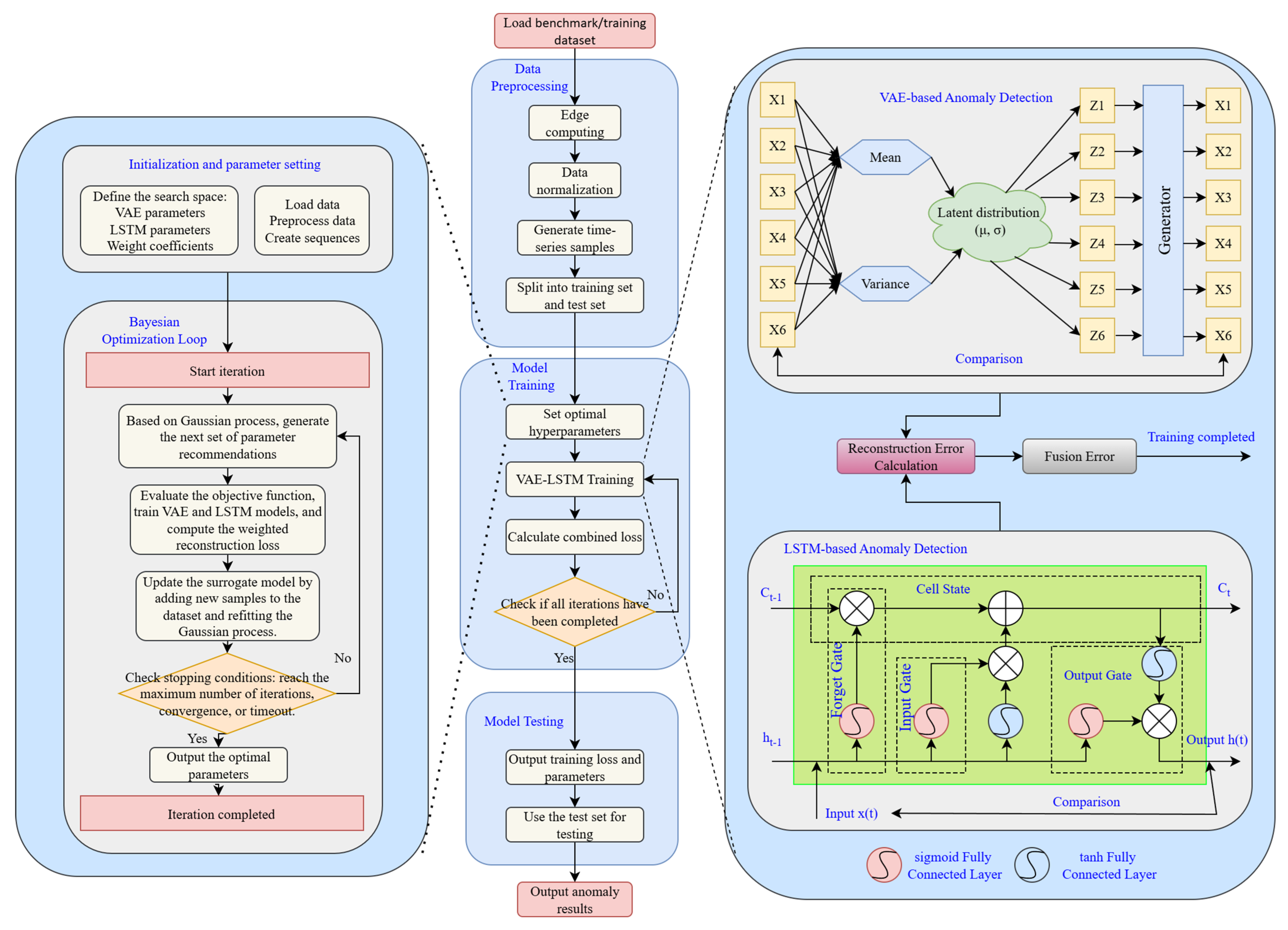
As shown in Figure 2, the overall detection framework consists of three stages:
Data preprocessing: raw signals are normalized, denoised, and segmented into time windows to form structured time-series samples.
Model training: VAE–LSTM is trained using normal operational data, ensuring the model captures baseline system behavior.
Model testing: unseen signals are evaluated by comparing reconstruction and prediction errors against adaptive thresholds to determine anomalies.
This design ensures that the proposed framework not only reduces false alarms caused by redundant sensor noise but also improves sensitivity to stealthy and low-frequency cyberattacks, thereby providing reliable protection for wastewater treatment operations.

2.2. Data Preprocessing

In the context of anomaly diagnosis for water treatment systems, edge computing, data normalization, and data partitioning are the key steps to ensure effective training of the VAE-LSTM model and accurate anomaly detection. In real-world water treatment systems, high-frequency data acquisition is easily affected by electromagnetic noise, packet loss, and other forms of data corruption, and often contains a large amount of redundancy. Moreover, the differences in dimension and scale among water treatment data may cause imbalances in feature weights during model training, leading to inefficiency.
Edge computing is primarily used to process normal operational signals from the water treatment system at the sensor-near edge, where high-frequency data is initially handled. For example, low-pass filters can be applied to remove electromagnetic interference and other high-frequency noise, preventing bus bandwidth occupation or contamination of downstream data. Additionally, incomplete or failed checksum protocol frames can be detected and discarded in time, ensuring that only clean samples are transmitted to the cloud for training.
Data normalization addresses the diversity of sensor categories and the multidimensional nature of water treatment signals, which often vary greatly in scale and numerical range. Normalization maps features into the same range, enabling the model to learn temporal patterns of each feature fairly, avoiding dominance by features with larger numerical values. It also accelerates model convergence, improves VAE-LSTM training efficiency, reduces training time, and makes the model better suited for large-scale, high-frequency water treatment data. The formula is as follows:
x = x x min x max x min
where x is the normalized data, x is the original data, x min is the minimum value of the original data, and x max is the maximum value of the original data [20].

2.3. Variational Autoencoder for Anomaly Detection

The Variational Autoencoder (VAE) extends the traditional autoencoder by introducing a probabilistic latent variable model, which enables not only dimensionality reduction and feature extraction but also the learning of the underlying data distribution. This property is particularly important for anomaly detection, since distinguishing between normal and abnormal signals often depends on distributional deviations. As illustrated in Figure 2, the VAE consists of an encoder, a latent variable layer, and a decoder [21].
Let x i denote the original multidimensional water treatment data. The encoder maps x i into a latent variable z characterized by a mean μ and variance σ2, which are assumed to follow a Gaussian distribution:
p θ x i | z = i = 1 D p θ x i | z
where z is the latent variable and θ represents model parameters. To ensure differentiability during training, the reparameterization trick is applied:
z = μ + σ ε
where ⊙ denotes element-wise multiplication. The latent variable z is then passed through the decoder function f θ ( Z ) to reconstruct the input:
X ^ = f θ Z
The total loss is calculated from the reconstructed multi-dimensional data and the initial input data as shown in Equation (5). Subsequently, the reconstruction error and KL divergence are computed as shown in Equations (6)–(7).
L X = M S E + K L
E q Z | X log p X | Z 1 2 i = 1 n X i X ^ i 2
K L q Z | X | | p Z = 1 2 i = 1 n μ i 2 + σ i 2 log σ i 2 1
Among them, the reconstruction error is approximately equivalent to the MSE, and KL represents the divergence. When a new and unknown signal from the water treatment system is input into the trained model, the reconstruction error is obtained by comparing the reconstructed data with the input data, and then compared with the preset threshold. Let the reconstruction error of normal data be denoted as Enormal. Based on this, the values of μ E and σ E can be calculated, and the threshold T is derived as shown in Equation (8). By comparing T with the calculated error E, if E is larger than T, the signal is considered normal; otherwise, it is considered abnormal. The specific process is illustrated in Figure 3.
T = μ E + 3 σ E ,   μ E = E E n o r m a l ,   σ E = s t d E n o r m a l

2.4. Anomaly Detection Method Based on Long Short-Term Memory Recurrent Neural Network

The Long Short-Term Memory (LSTM) network is a variant of the recurrent neural network (RNN) designed to mitigate the vanishing gradient problem through a gating mechanism, including the input gate, forget gate, output gate, and cell state [22]. This structure enables the effective capture of both short-term and long-term dependencies in time-series data, which is crucial for modeling process dynamics in wastewater treatment plants. The model structure is shown in Figure 2.
Formally, the input gate regulates the extent to which new information C ˜ t (candidate state) is added to the cell state, the forget gate controls how much information from the previous state Ct−1 is retained, and the output gate determines the portion of the updated state to pass forward as the hidden state h t :
i t = σ W i h t 1 , x t + b i
C ˜ t = tanh W c h t 1 , x t + b c
f t = σ W f h t 1 , x t + b f
C t = f t C t 1 + i t C ˜ t
o t = σ W o h t 1 , x t + b o
h t = o t tanh C t
where σ(⋅) is the sigmoid activation, ⊙ denotes element-wise multiplication, and W and b are trainable parameters. These gating operations allow the LSTM to preserve long-term correlations (e.g., gradual water-level drifts) while being responsive to short-term fluctuations (e.g., actuator switching).
For anomaly detection, we adopt an LSTM autoencoder. In the training phase, sequences of normal operating data are encoded into hidden representations hT, and then reconstructed by a decoder LSTM. The model parameters are optimized to minimize the reconstruction error ensuring the autoencoder learns only the temporal patterns of normal system behavior.
In the detection phase, unseen sequences are fed into the trained model. Their reconstruction errors are compared against a detection threshold T, defined from the mean and variance of reconstruction errors under normal conditions. If the error E > T, the sequence is flagged as anomalous; otherwise, it is considered normal. This procedure is illustrated in Figure 4, where both “Yes (Anomaly)” and “No (Normal)” decision paths are now explicitly shown.

2.5. Combined Anomaly Detection Method for Water Treatment Data Based on VAE-LSTM

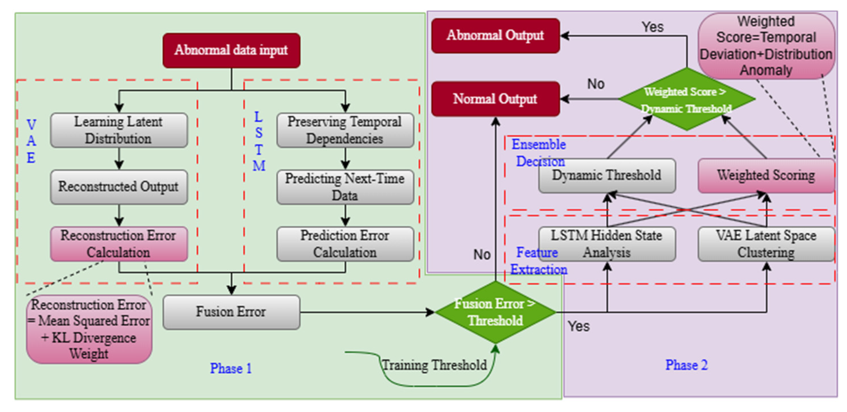
The combined VAE-LSTM method for detecting anomalies in water treatment data is mainly divided into two stages, as shown in Figure 5.
Stage 1: Error computation and preliminary fusion.
Reconstruction errors are first calculated independently by the VAE (feature distribution learning) and the LSTM (temporal dependency modeling). A weighted combination of the two errors provides an initial anomaly score.
Stage 2: Adaptive decision with dynamic thresholds.
Unlike fixed thresholds used in traditional methods, a dynamic threshold is introduced to adapt to variations in data distributions over time. The threshold is updated periodically based on the fused error statistics, ensuring sensitivity to gradual shifts and robustness against noise. In addition, a weighted scoring mechanism is designed to balance spatial and temporal contributions:
D D = E V A E t max E V A E
D T = E LSTM t max E L S T M
S C O R E = α × D D + 1 α × D T
where D D represents the distribution-based anomaly degree, D T the temporal deviation degree, and α is a tunable weight.
This design ensures that anomalies manifesting as instantaneous sensor deviations (e.g., false readings) are captured by the VAE, while temporal irregularities are detected by the LSTM. The integration of reconstruction and prediction perspectives significantly enhances robustness against diverse fault modes in wastewater treatment plants.

2.6. Algorithm Performance Evaluation Metrics

In anomaly detection for water treatment systems, metrics such as Accuracy, Precision, Recall, F1, FPR, and FNR quantify the algorithm’s capability in processing sensor data from multiple perspectives, including overall classification, reliability of anomaly prediction, detection comprehensiveness, overall performance, and the risk of false alarms or missed detections. By selecting the algorithm with the optimal F1 -Score, a balance can be achieved between false positives (low FPR, reducing unnecessary actuator interventions) and false negatives (low FNR, ensuring water treatment system safety). This approach ensures real-time sensor monitoring and accurate actuator responses, enabling coordinated improvement of normal operation and operational efficiency, and provides critical quantitative guidance for stable and reliable operation of water treatment systems as well as algorithm selection [23].
Accuracy = TP + TN TP + TN + FP + FN
Precision = TP TP + FP
Recall = TP TP + FN
F 1 = 2 × Precision × Recall Precision + Recall
FPR = FP FP + TN
FNR = FN TP + FN

3. Experimental Platform

In this study, the SWaT and WADI datasets were used to validate the performance of the proposed algorithm. These datasets were collected and open-sourced by the iTrust research group at the Singapore University of Technology and Design (SUTD), containing both normal and attack-induced multi-dimensional sensor signal data [24,25].
The SWaT dataset was collected from a water treatment testbed launched in 2015, covering six stages of water treatment: raw water intake, chemical dosing, ultrafiltration, UV disinfection and dechlorination, reverse osmosis, and backwash. The platform’s network components include PLCs, HMI, SCADA workstations, and a Historian that records sensor data. Table 1 lists each step of the SWaT water treatment system along with its monitored sensors and actuators. The sensors include flow meters, level sensors, chemical concentration sensors, differential pressure sensors, and pressure sensors, while the actuators include electric control valves, electric pumps, and UV lamps. Figure 6 and Figure 7 illustrate the variations in the FIT101 and MV101 sensors under attack scenarios within the SWaT system.
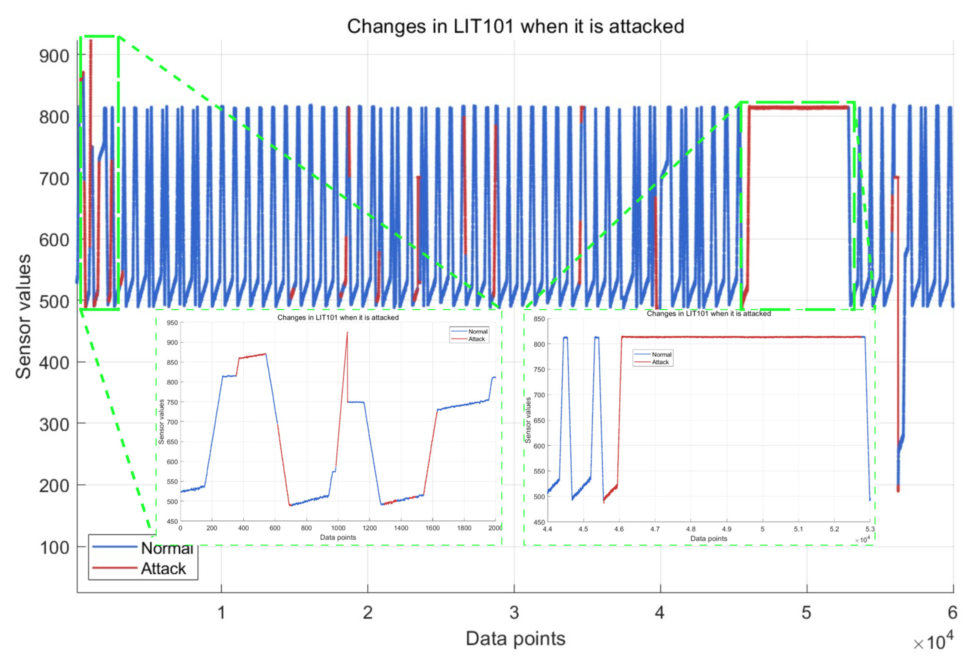
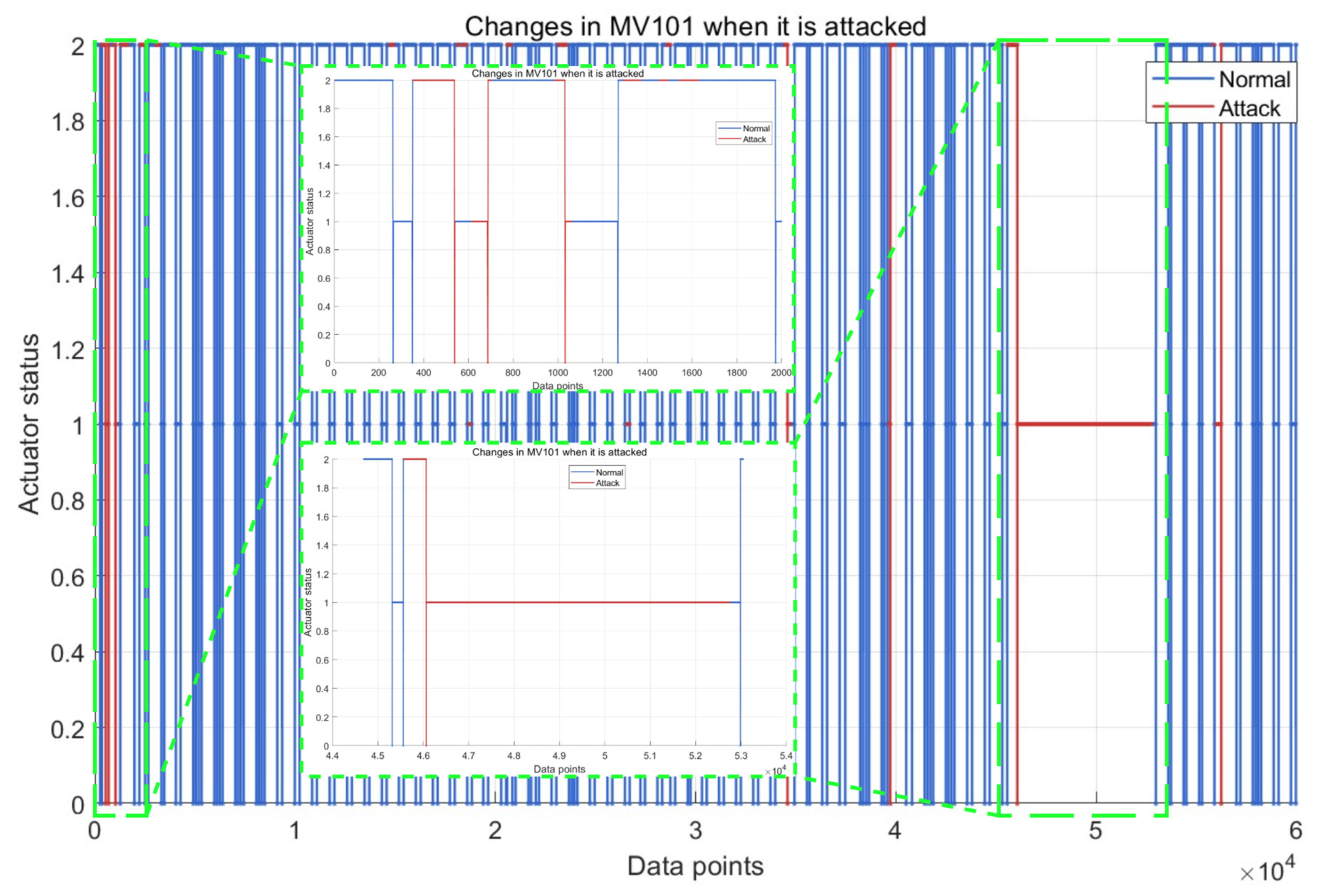
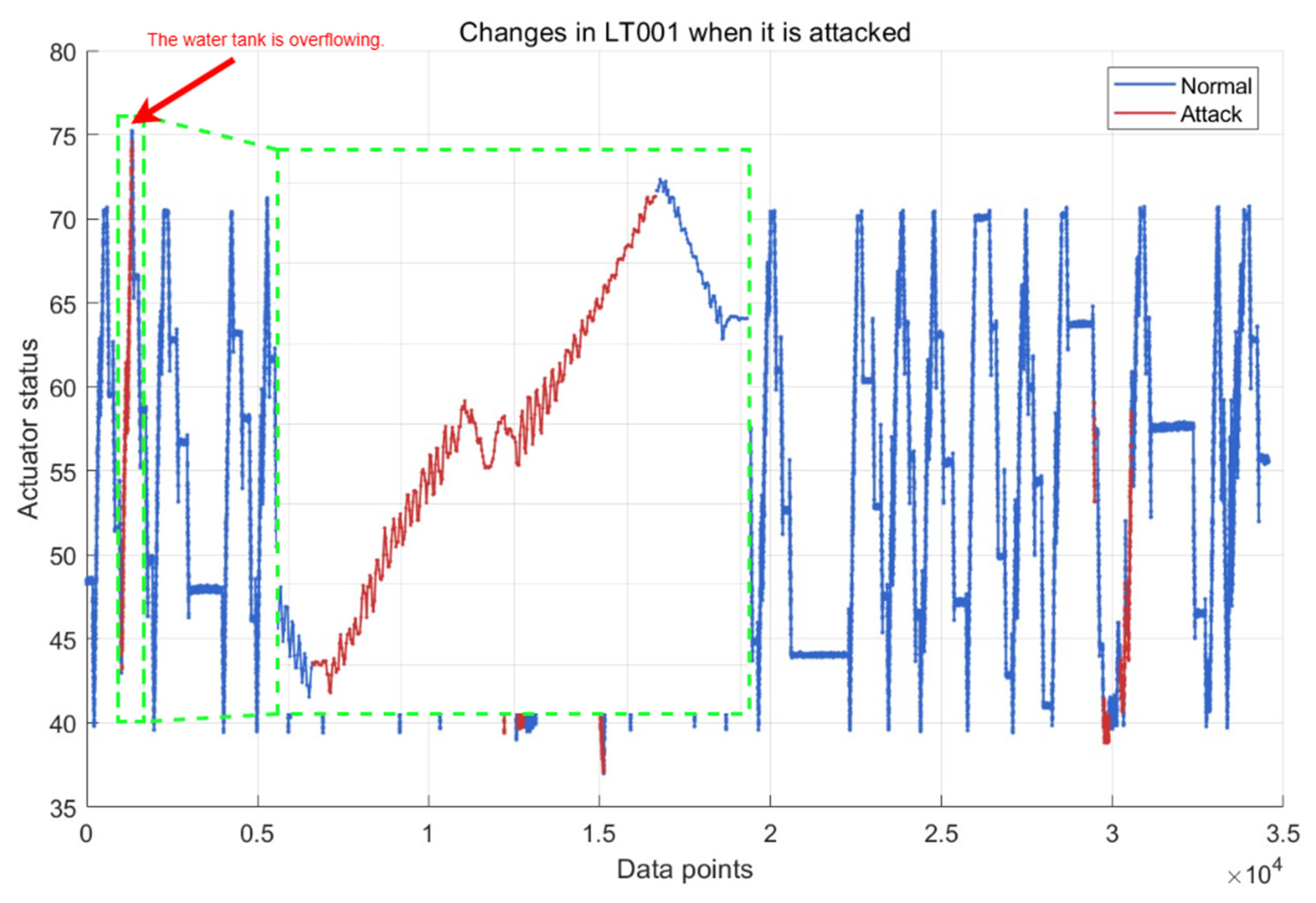
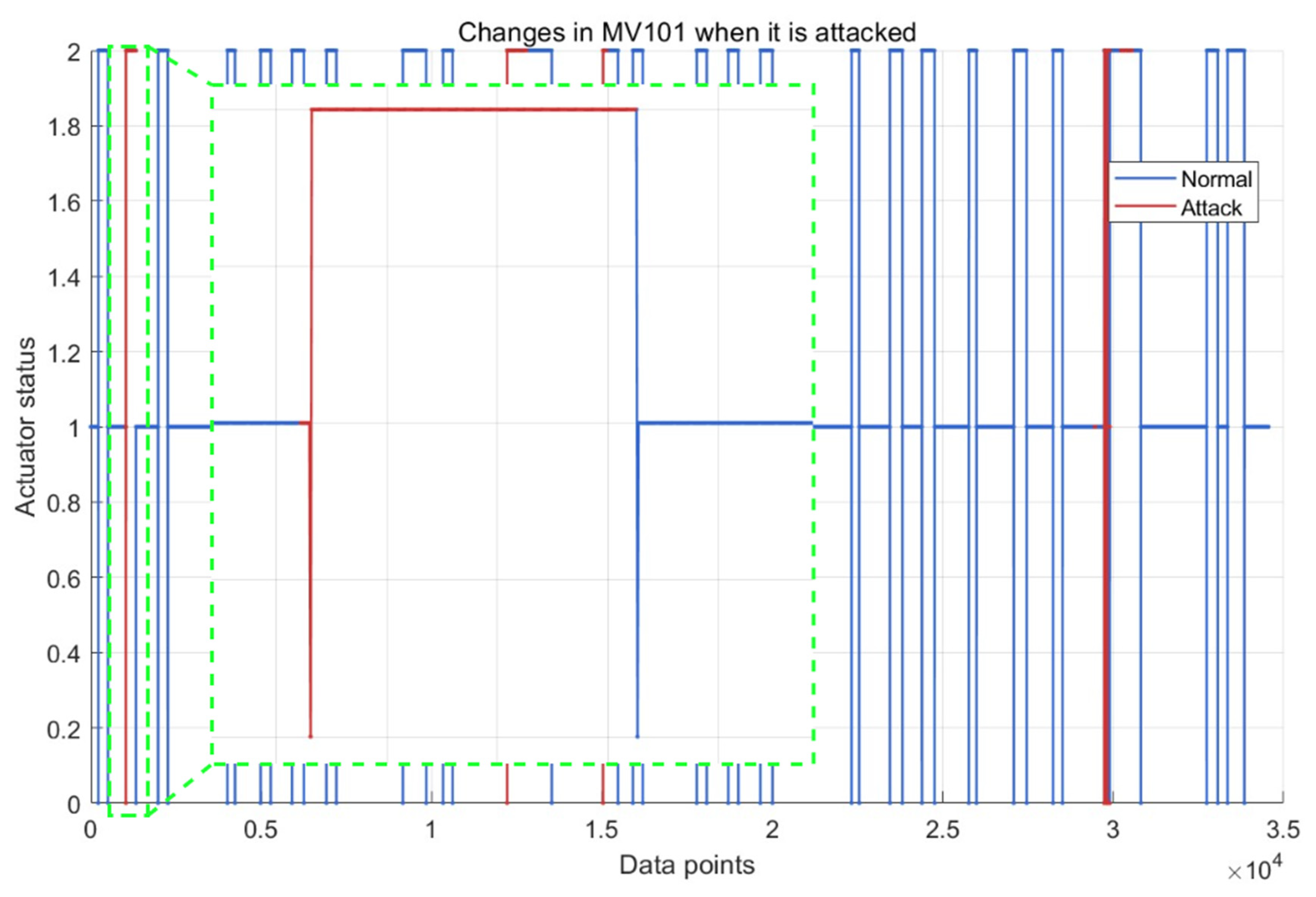
The WADI dataset was also developed by the iTrust research group at the Singapore University of Technology and Design (SUTD). It includes two elevated water tanks, six consumer water tanks, two raw water tanks, and one return water tank, equipped with a chemical dosing system, booster pumps and valves, instrumentation, and analyzers. WADI incorporates a portion of the reverse osmosis permeate and raw water from SWaT, forming a complete and realistic water treatment, storage, and distribution network. The specific components are listed in Table 2. Figure 8 and Figure 9 illustrate the variations in the LT101 and MV101 sensors under attack scenarios in the WADI system.

4. Experimental Environment and Optimal Hyperparameter Calculation

4.1. Experimental Environment

The experiments in this study were conducted on a Windows 10 operating system with an Intel Core i5-13600KF CPU and an RTX 4060 Ti 8GB GPU (Intel, Santa Clara, CA, USA). The main tools used include PyTorch 2.6.0 (deep learning framework), Pandas 2.2.3 (data processing), Scikit-learn 1.6.1 (model evaluation), and Scikit-optimize 0.10.2 (hyperparameter optimization).
Regarding datasets, the SWaT and WADI water treatment system datasets were used, as summarized in Table 3. The SWaT dataset contains 11 days of continuous operation data from a six-stage water treatment system, with the first 7 days representing normal operation and the remaining 4 days including intermittent network attacks. The dataset comprises 495,000 normal samples and 449,919 attack samples. After downsampling, the training and testing sets contain 99,000 and 89,983 samples, respectively. The attack model launched 41 attacks through the CPS attack intention space.
The WADI dataset contains 16 days of water treatment system data, with 14 days of normal operation and 2 days of intermittent attacks. This dataset includes 1,209,600 normal samples and 172,806 attack samples. After downsampling, the training and testing sets contain 241,920 and 34,561 samples, respectively, and the attack model launched 15 attacks.

4.2. Hyperparameter Optimization Calculation

4.2.1. Principle of Bayesian Optimization

Bayesian Optimization is a probabilistic model-based global optimization method, particularly suitable for black-box optimization problems where the objective function is expensive to evaluate and derivative information is unavailable [26]. The specific process is also illustrated in Figure 2.
Initially, random starting points are selected in the parameter space, and the corresponding values of the objective function are computed. Iteratively, a surrogate model in Bayesian Optimization is chosen as a Gaussian Process (GP). In the GP, the objective function f is assumed to follow a multivariate Gaussian distribution, with mean function m x and covariance function defined as Equation (24).
k x , x = σ 2 exp x x 2 2 l 2
Here, σ 2 denotes the signal variance, which controls the overall amplitude of the objective function, and l represents the length scale, which governs the smoothness of the objective function. The hyperparameters of the Gaussian Process are estimated via maximum likelihood estimation (MLE). The objective of MLE is to maximize the likelihood function, as shown in Equation (25).
log p y X , θ = 1 2 y T K + σ n 2 I 1 y 1 2 log K + σ n 2 I n 2 log 2 π
Here, y denotes the observed values of the objective function, X represents the corresponding parameter points, K is the covariance matrix, σ n 2 is the noise variance, I is the identity matrix, n is the number of observations, and θ represents the hyperparameters.
Next, the acquisition function is constructed. The acquisition function guides the algorithm in selecting the next most promising sampling point in the parameter space. Since the function f ( x ) follows a Gaussian distribution, the Expected Improvement (EI) function can be expressed as Equation (26).
a E I x = f min μ x Φ f min μ x σ x + σ x ϕ f min μ x σ x
Here, f min denotes the currently observed minimum of the objective function, and f x is the predicted function value at the parameter point x. μ(x) and σ(x) represent the predicted mean and standard deviation of the function value at x, respectively. Φ and φ denote the cumulative distribution function (CDF) and probability density function (PDF) of the standard normal distribution, respectively.

4.2.2. Bayesian Optimization Objectives and Hyperparameters

The main hyperparameters optimized by Bayesian Optimization include: the VAE latent space dimension (smaller values yield compact representations but may lose information, larger values retain more information at higher complexity); the number of neurons in VAE encoder and decoder hidden layers (feature extraction capacity); the KL divergence weight β in VAE (controls closeness to standard normal distribution); LSTM network depth (captures abstract temporal features); LSTM hidden state dimension (memory capacity for temporal information); use of bidirectional LSTM (captures forward and backward context); and dropout rate between LSTM layers (prevents overfitting), escription and Range of Hyperparameters for Bayesian Optimization are shown in Table 4.
The optimization objective is T_loss, as defined in the corresponding equation. Bayesian Optimization automatically finds the optimal combination of these hyperparameters, which is more efficient than manual tuning and may discover parameter configurations that are difficult for humans to conceive. Compared with manual tuning, Bayesian Optimization can improve the VAE’s focus on latent representations and probability distributions, as the optimized parameters affect feature compression and reconstruction accuracy. For the LSTM, which focuses on temporal dependency modeling, the hyperparameters influence the ability to capture sequential patterns. Bayesian Optimization considers both sets of parameters simultaneously, finding an optimal balance between them.
T l o s s = a E V A E + b K L + c E L S T M
Here, Tloss represents the overall loss; KL denotes the VAE divergence; and a, b, and c are weighting parameters, with b set to 0.1.

4.2.3. Optimal Hyperparameter Calculation

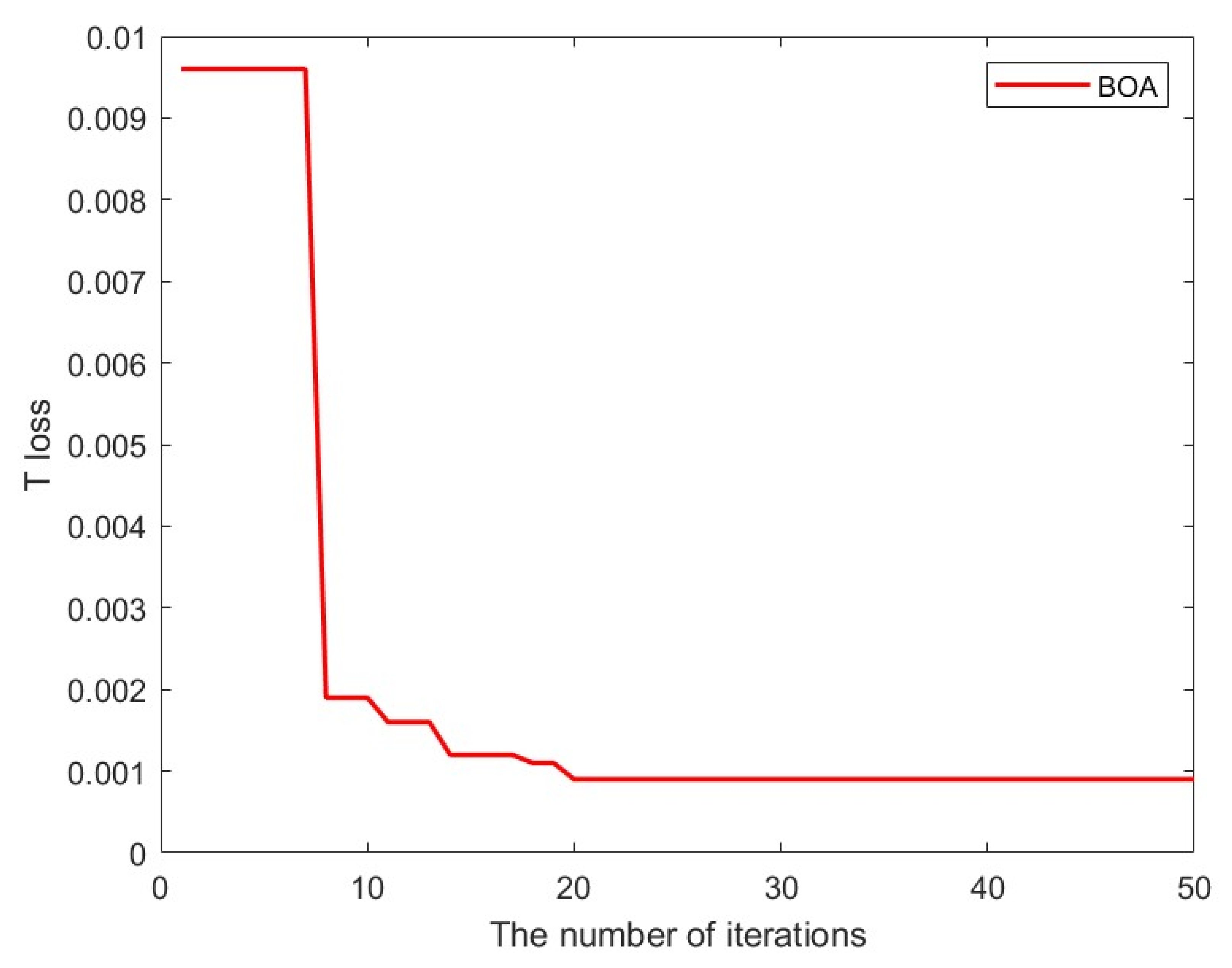
Bayesian Optimization was performed for 50 iterations using T loss as the objective function. Multiple hyperparameters were optimized simultaneously. The optimal parameters are listed in Table 5.
As shown in Figure 10, during Bayesian Optimization, the overall loss T_loss begins to gradually decrease from the 7th iteration and approaches 0.001. This indicates that, when training on the normal water treatment signal dataset, selecting the optimal hyperparameters via Bayesian Optimization reduces the overall loss and reconstruction error. Consequently, when testing on the attack dataset, the feature points are more pronounced, and the reconstruction error values become clearly distinguishable, enabling the detection of whether the water treatment system has been subjected to a cyberattack.

4.3. Model Training

The VAE-LSTM algorithm was trained on the normal operation dataset of the water treatment system using the optimal hyperparameter values.
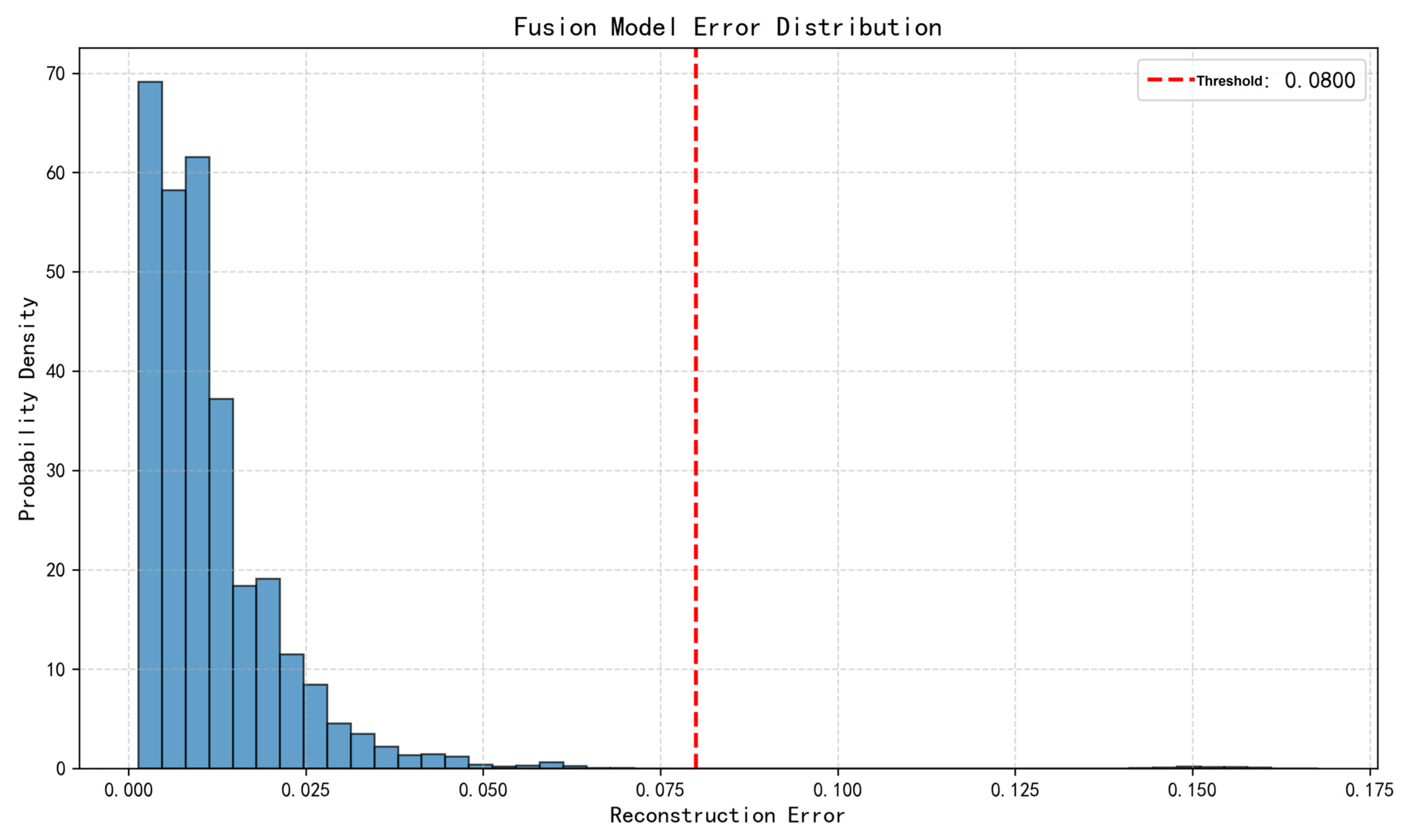
As shown in Figure 11, most of the reconstruction errors for the training data fall below 0.08. Through multiple training experiments, it was found that an initial threshold of 0.08 yields the best performance. Therefore, 0.08 was selected as the preliminary threshold and used as the training threshold in the first stage of the VAE-LSTM-based hybrid method for detecting anomalies in water treatment data.

5. Algorithm Experiments and Comparisons

5.1. Comparison of Algorithms and Ablation Study

To evaluate the performance of the VAE-LSTM algorithm, anomaly detection results using a standalone VAE and a standalone LSTM were compared. The hyperparameters of the individual VAE and LSTM models were set the same as those in the hybrid model. Additionally, the results were compared with single-threshold methods such as Isolation Forest (IF) [27] and One-Class Support Vector Machine (OCSVM) [28]. The hyperparameters for these algorithms are listed in Table 6 and Table 7.
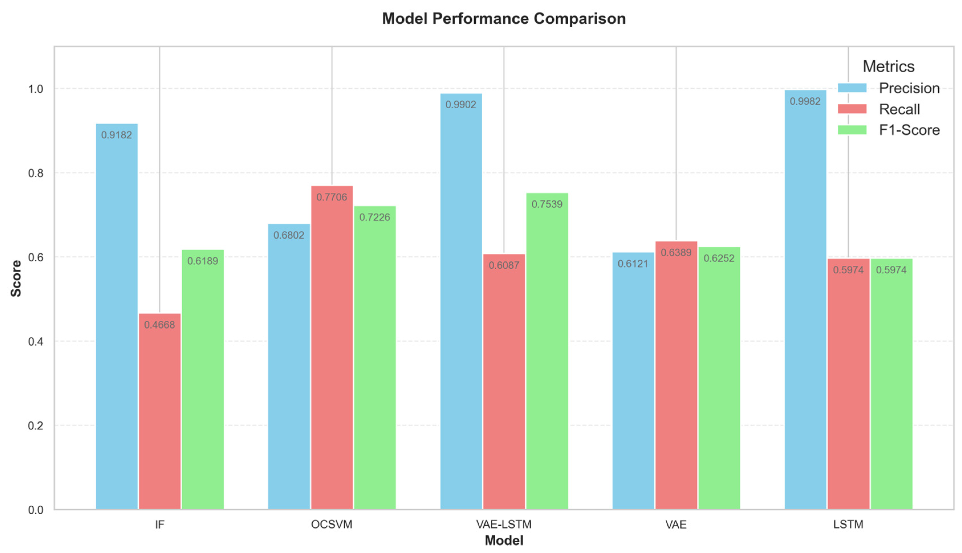
As shown in Figure 12, the VAE-LSTM achieves the highest F1-Score of 0.7539 among all models. The F1-Score, as the harmonic mean of precision and recall, directly reflects the model’s ability to balance ‘precision’ and ‘completeness.’ The F1 value of VAE-LSTM is significantly higher than other models, such as OCSVM (0.7228), VAE (0.6262), LSTM (0.5974), and IF (0.6109), indicating that it reduces both false positives and false negatives, achieving the best overall performance.
The precision of VAE-LSTM reaches 0.9901, nearly 1, meaning that over 99% of its predicted anomalies are indeed anomalies. In comparison, while LSTM shows high precision, its recall is extremely low, leading to severe false negatives; OCSVM has a precision of only 0.6802, resulting in more false positives. VAE-LSTM maintains high precision while also achieving better recall than LSTM, thus avoiding many false negatives. Its recall is 0.5988, slightly lower than OCSVM, but given its very high precision, the balance between false negative and false positive risks is superior. While OCSVM’s high recall comes at the cost of low precision, potentially causing numerous unnecessary interventions in the water treatment system, VAE-LSTM reduces false positives through high precision and effectively captures most anomalies, making it more suitable for practical applications.

5.2. Comparison of Training and Testing Time

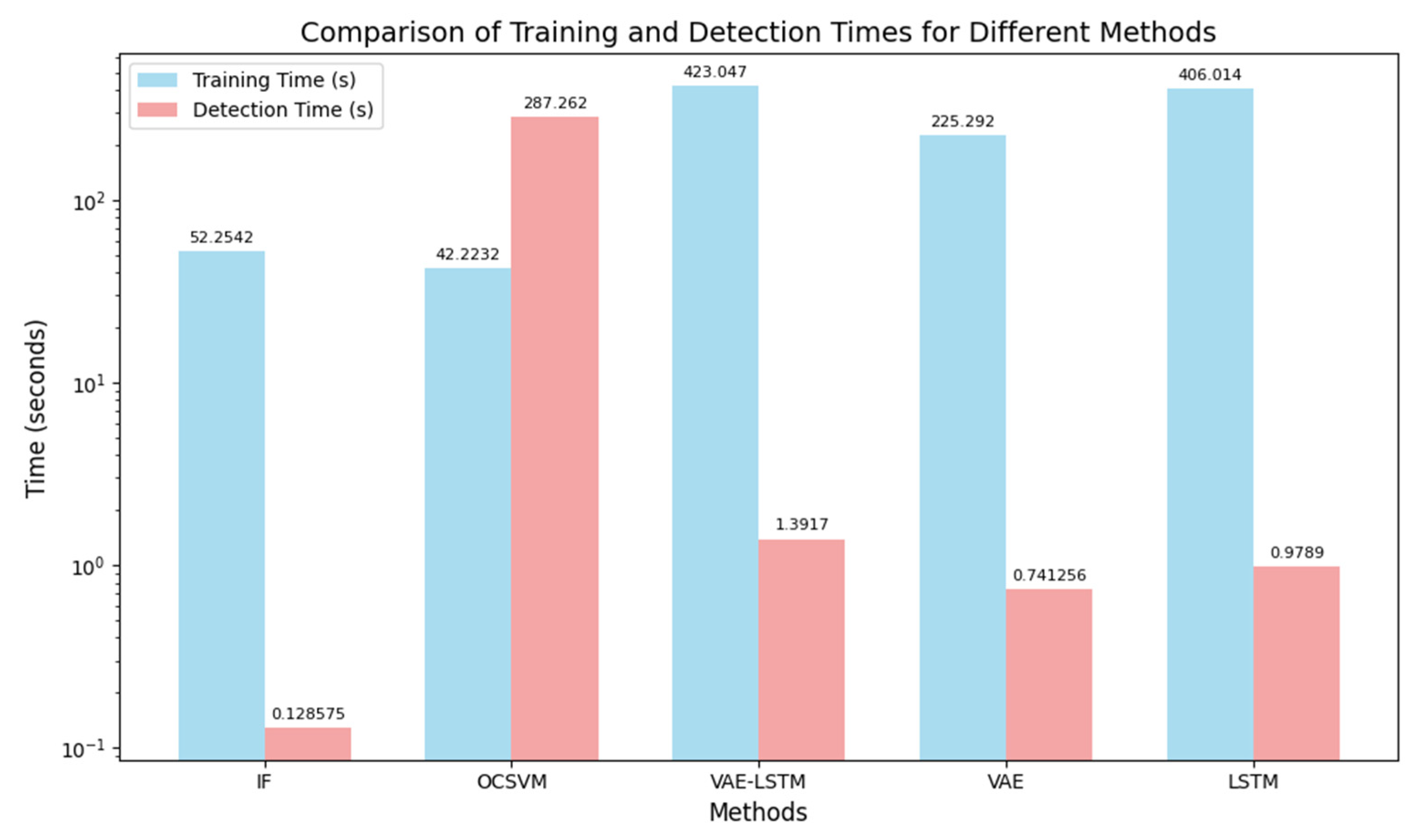
Rapid detection of anomalies in water treatment system data is a critical capability. Therefore, this study compares the training and testing times of IF, OCSVM, VAE-LSTM, VAE, and LSTM. Since these times depend on the device’s processor, the comparison primarily focuses on the relative efficiency of the algorithms.
Considering the core requirements of real-time water quality data acquisition by sensors and rapid actuator intervention in water treatment systems, Figure 13 shows that VAE-LSTM achieves the highest F1-Score among all models, with the best balance between precision and recall. It significantly outperforms OCSVM (high false positives), LSTM (high false negatives), and VAE/IF (inferior overall performance). In terms of efficiency, the training time is 423.04 s on an RTX 4060 Ti GPU. This is a one-time offline cost and does not affect online operation. For detection, the total inference time for the entire SWaT test set (89,983 samples) is 1.39 s, which translates to a per-sample detection time well below real-time requirements. In contrast, OCSVM has very long detection times, IF shows poor performance, and VAE/LSTM have insufficient overall performance (F1 of 0.6262 and 0.5974, respectively). Therefore, VAE-LSTM achieves the best trade-off between “accurate anomaly detection (reducing false positives and negatives, ensuring water quality and system stability)” and “real-time data processing, meeting sensor second-level updates and actuator rapid response requirements”. As a result, the data in Figure 13 supports VAE-LSTM as the optimal algorithm for water treatment anomaly detection, with performance and time characteristics perfectly aligned with the real-time, accuracy, and stability demands of water treatment scenarios.

5.3. WADI Water Treatment System

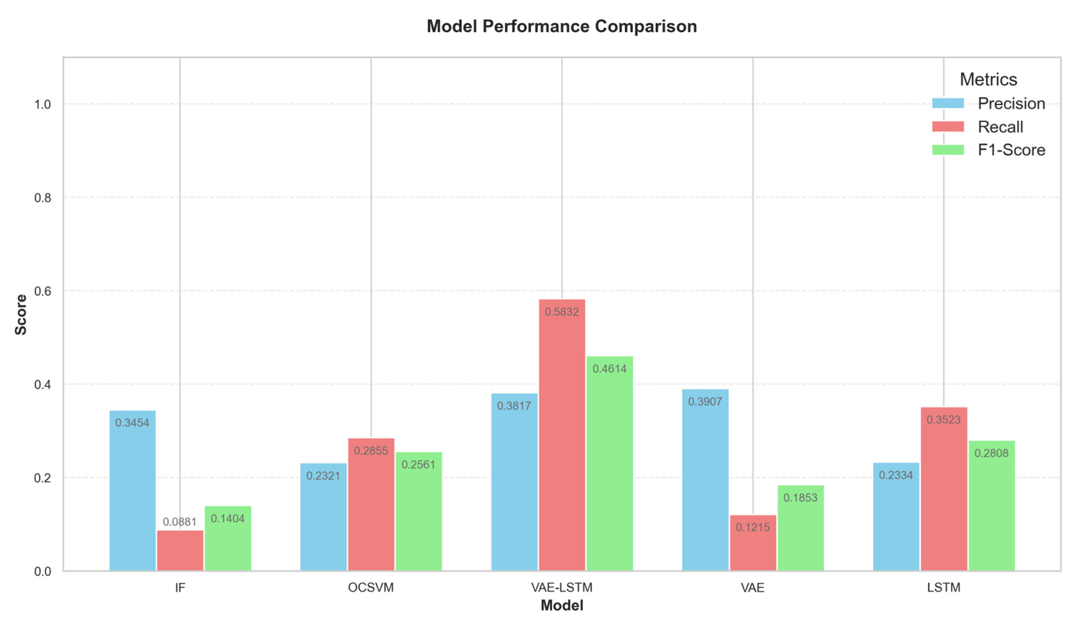
On the high-dimensional WADI dataset, which features stealthy attacks, the generalization performance of five algorithms—IF, OCSVM, VAE, LSTM, and VAE-LSTM—was compared, as shown in Figure 14.
The experiments indicate that VAE-LSTM achieves the best F1-Score (0.5832), leveraging its advantages in “high-dimensional feature generalization + temporal dynamic modeling”. Specifically, the VAE component effectively generalizes complex multi-sensor features, reducing misclassification caused by distribution differences, while the LSTM captures temporal dependencies in stealthy attacks, improving recall for weak anomalies. The combination not only achieves a good balance between precision (0.3817) and recall (0.4614) but also demonstrates strong adaptability to high-dimensional time-series data and complex operating conditions.

6. Conclusions

This study developed a VAE-LSTM hybrid anomaly detection framework that combines the VAE’s ability to learn latent data distributions with the LSTM’s strength in modeling temporal dependencies, effectively addressing the challenge of detecting both temporal and latent feature anomalies in water treatment systems. In terms of performance, the model demonstrates excellent accuracy and F1-Score while meeting the requirements of both real-time and high-precision scenarios. Experimental results validate its effectiveness, providing a practical and implementable solution for intelligent monitoring in industrial water treatment with significant real-world value.
Nevertheless, some limitations should be acknowledged. The deep architecture may be prone to overfitting when trained on smaller or highly imbalanced datasets. While robustness has been demonstrated on SWaT and WADI, additional testing under noisy sensor conditions and cross-plant deployments is still needed to ensure wider applicability. Moreover, although the current computational cost is acceptable, further optimization is required for highly resource-constrained environments.
Future research will therefore focus on model lightweighting to reduce resource consumption, enhancing data generalization to adapt to more operating conditions, and integrating edge computing for “edge-to-cloud” collaboration. These directions will further improve system usability and robustness, supporting technological innovation and upgrading in the industrial water treatment sector toward intelligence, sustainability, and efficiency.

Author Contributions

Conceptualization, X.L. and X.Z.; methodology, X.Z.; software, X.Z.; validation, X.L. and Z.G.; formal analysis, X.L.; investigation, X.L. and Z.G.; resources, Z.G.; data curation, X.Z.; writing—original draft preparation, X.L. and X.Z.; writing—review and editing, X.L.; visualization, X.Z.; supervision, X.L.; project administration, X.L.; funding acquisition, X.L. All authors have read and agreed to the published version of the manuscript.

Funding

This research was supported by the National Science Foundation of China (12305280).

Data Availability Statement

The original contributions presented in this study are included in the article. Further inquiries can be directed to the corresponding author.

Conflicts of Interest

The authors declare no conflicts of interest.

References

  1. Cordeiro, S.; Ferrario, F.; Pereira, H.X.; Ferreira, F.; Matos, J.S. Water Reuse, a Sustainable Alternative in the Context of Water Scarcity and Climate Change in the Lisbon Metropolitan Area. Sustainability 2023, 15, 12578. [Google Scholar] [CrossRef]
  2. Solanki, S.D.; Bhalani, J.; Ahmad, N. Exploring a Novel Strategy for Detecting Cyber-Attack by Using Soft Computing Technique: A Review. In Soft Computing Techniques and Applications. Advances in Intelligent Systems and Computing; Borah, S., Pradhan, R., Dey, N., Gupta, P., Eds.; Springer: Singapore, 2021; Volume 1248. [Google Scholar] [CrossRef]
  3. El Kafhali, S.; El Mir, I.; Hanini, M. Security Threats, Defense Mechanisms, Challenges, and Future Directions in Cloud Computing. Arch. Comput. Methods Eng. 2022, 29, 223–246. [Google Scholar] [CrossRef]
  4. Kaittan, K.H.; Mohammed, S.J. PLC-SCADA automation of inlet wastewater treatment processes: Design, implementation, and evaluation. J. Eur. Systèmes Autom. 2024, 57, 787–796. [Google Scholar] [CrossRef]
  5. Ning, S.; Hong, S. Programmable logic controller-based automatic control for municipal wastewater treatment plant optimization. Water Pract. Technol. 2022, 17, 378–384. [Google Scholar] [CrossRef]
  6. Gönen, S.; Sayan, H.H.; Yılmaz, E.N.; Üstünsoy, F.; Karacayılmaz, G. False data injection attacks and the insider threat in smart systems. Comput. Secur. 2020, 97, 101955. [Google Scholar] [CrossRef]
  7. Zhang, X.; Jiang, Z.; Ding, Y.; Ngai, E.C.; Yang, S.-H. Anomaly detection using isomorphic analysis for false data injection attacks in industrial control systems. J. Frankl. Inst. 2024, 361, 107000. [Google Scholar] [CrossRef]
  8. Zhang, J.; Tao, Y.; Li, M. Design of Industrial Gateway on Modbus TCP. Mach. Electron. 2014, 50–53. [Google Scholar] [CrossRef]
  9. Andrysiak, T.; Saganowski, Ł.; Maszewski, M.; Marchewka, A. Detection of Network Attacks Using Hybrid ARIMA-GARCH Model. In Advances in Dependability Engineering of Complex Systems. DepCoS-RELCOMEX 2017. Advances in Intelligent Systems and Computing; Zamojski, W., Mazurkiewicz, J., Sugier, J., Walkowiak, T., Kacprzyk, J., Eds.; Springer: Cham, Switzerland, 2018; Volume 582. [Google Scholar] [CrossRef]
  10. Gan, Z.; Zhou, X. Abnormal Network Traffic Detection Based on Improved LOF Algorithm. In Proceedings of the 2018 10th International Conference on Intelligent Human-Machine Systems and Cybernetics (IHMSC), Hangzhou, China, 25–26 August 2018; pp. 142–145. [Google Scholar] [CrossRef]
  11. Elnour, M.; Meskin, N.; Khan, K.; Jain, R. A Dual-Isolation-Forests-Based Attack Detection Framework for Industrial Control Systems. IEEE Access 2020, 8, 36639–36651. [Google Scholar] [CrossRef]
  12. Vos, K.; Peng, Z.; Jenkins, C.; Shahriar, R.; Borghesani, P.; Wang, W. Vibration-based anomaly detection using LSTM/SVM approaches. Mech. Syst. Signal Process. 2022, 169, 108752. [Google Scholar] [CrossRef]
  13. Nizan, O.; Tal, A. k-NNN: Nearest Neighbors of Neighbors for Anomaly Detection. In Proceedings of the 2024 IEEE/CVF Winter Conference on Applications of Computer Vision Workshops (WACVW), Waikoloa, HI, USA, 1–6 January 2024; pp. 1005–1014. [Google Scholar] [CrossRef]
  14. Cicceri, G.; Maisano, R.; Morey, N.; Distefano, S. A novel architecture for the smart management of wastewater treatment plants. In Proceedings of the 2021 IEEE International Conference on Smart Computing (SMARTCOMP), Irvine, CA, USA, 23–27 August 2021; pp. 392–394. [Google Scholar]
  15. Cicceri, G.; Maisano, R.; Morey, N.; Distefano, S. Swims: The smart wastewater intelligent management system. In Proceedings of the 2021 IEEE International Conference on Smart Computing (SMARTCOMP), Irvine, CA, USA, 23–27 August 2021; IEEE: New York, NY, USA; pp. 228–233. [Google Scholar]
  16. Garcia-Alvarez, D.; Fuente, M.J.; Vega, P.; Sainz, G. Fault Detection and Diagnosis using Multivariate Statistical Techniques in a Wastewater Treatment Plant. IFAC Proc. Vol. 2009, 42, 952–957. [Google Scholar] [CrossRef]
  17. Hochreiter, S.; Schmidhuber, J. Long Short-Term Memory. Neural Comput. 1997, 9, 1735–1780. [Google Scholar] [CrossRef] [PubMed]
  18. Lima, L.O.M.; Goncalves, L.C.; Menezes, G.C.; de Oliveira, L.S. IoT-based Wireless Sensor Networks for Monitoring Drinking Water Treatment Plants. In Proceedings of the 2024 Symposium on Internet of Things (SIoT), Rio de Janeiro, Brazil, 15–18 October 2024; pp. 1–5. [Google Scholar] [CrossRef]
  19. Singh, M.; Ahmed, S. IoT based smart water management systems: A systematic review. Mater. Today Proc. 2021, 46 Pt 11, 5211–5218. [Google Scholar] [CrossRef]
  20. Wang, X.; Li, Y.; Qiao, Q.; Tavares, A.; Liang, Y. Water Quality Prediction Based on Machine Learning and Comprehensive Weighting Methods. Entropy 2023, 25, 1186. [Google Scholar] [CrossRef] [PubMed]
  21. Nguyen, H.H.; Nguyen, C.N.; Dao, X.T.; Duong, Q.T.; Pham Thi Kim, D.; Pham, M.-T. Variational autoencoder for anomaly detection: A comparative study. arXiv 2024, arXiv:2408.13561. [Google Scholar] [CrossRef]
  22. Greff, K.; Srivastava, R.K.; Koutnik, J.; Steunebrink, B.R.; Schmidhuber, J. LSTM: A Search Space Odyssey. IEEE Trans. Neural Netw. Learn. Syst. 2017, 28, 2222–2232. [Google Scholar] [CrossRef] [PubMed]
  23. Padilla, R.; Netto, S.L.; da Silva, E.A.B. A Survey on Performance Metrics for Object-Detection Algorithms. In Proceedings of the 2020 International Conference on Systems, Signals and Image Processing (IWSSIP), Niteroi, Brazil, 1–3 July 2020; pp. 237–242. [Google Scholar] [CrossRef]
  24. Goh, J.; Adepu, S.; Junejo, K.N.; Mathur, A. A dataset to support research in the design of secure water treatment systems. In Conference on Research in Cyber Security; Springer: Singapore, 2016. [Google Scholar]
  25. Ahmed, C.M.; Palleti, V.R.; Mathur, A.P. WADI: A water distribution testbed for research in the design of secure cyber physical systems. In Proceedings of the 3rd International Workshop on Cyber-Physical Systems for Smart Water Networks (CySWATER 2017), Pittsburgh, PA, USA, 21 April 2017; pp. 25–28. [Google Scholar]
  26. Papenmeier, L.; Poloczek, M.; Nardi, L. Understanding High-Dimensional Bayesian Optimization. arXiv 2025, arXiv:2502.09198. [Google Scholar]
  27. Al Farizi, W.S.; Hidayah, I.; Rizal, M.N. Isolation Forest Based Anomaly Detection: A Systematic Literature Review. In Proceedings of the 2021 8th International Conference on Information Technology, Computer and Electrical Engineering (ICITACEE), Semarang, Indonesia, 23–24 September 2021; pp. 118–122. [Google Scholar] [CrossRef]
  28. Miao, X.; Liu, Y.; Zhao, H.; Li, C. Distributed Online One-Class Support Vector Machine for Anomaly Detection Over Networks. IEEE Trans. Cybern. 2019, 49, 1475–1488. [Google Scholar] [CrossRef] [PubMed]
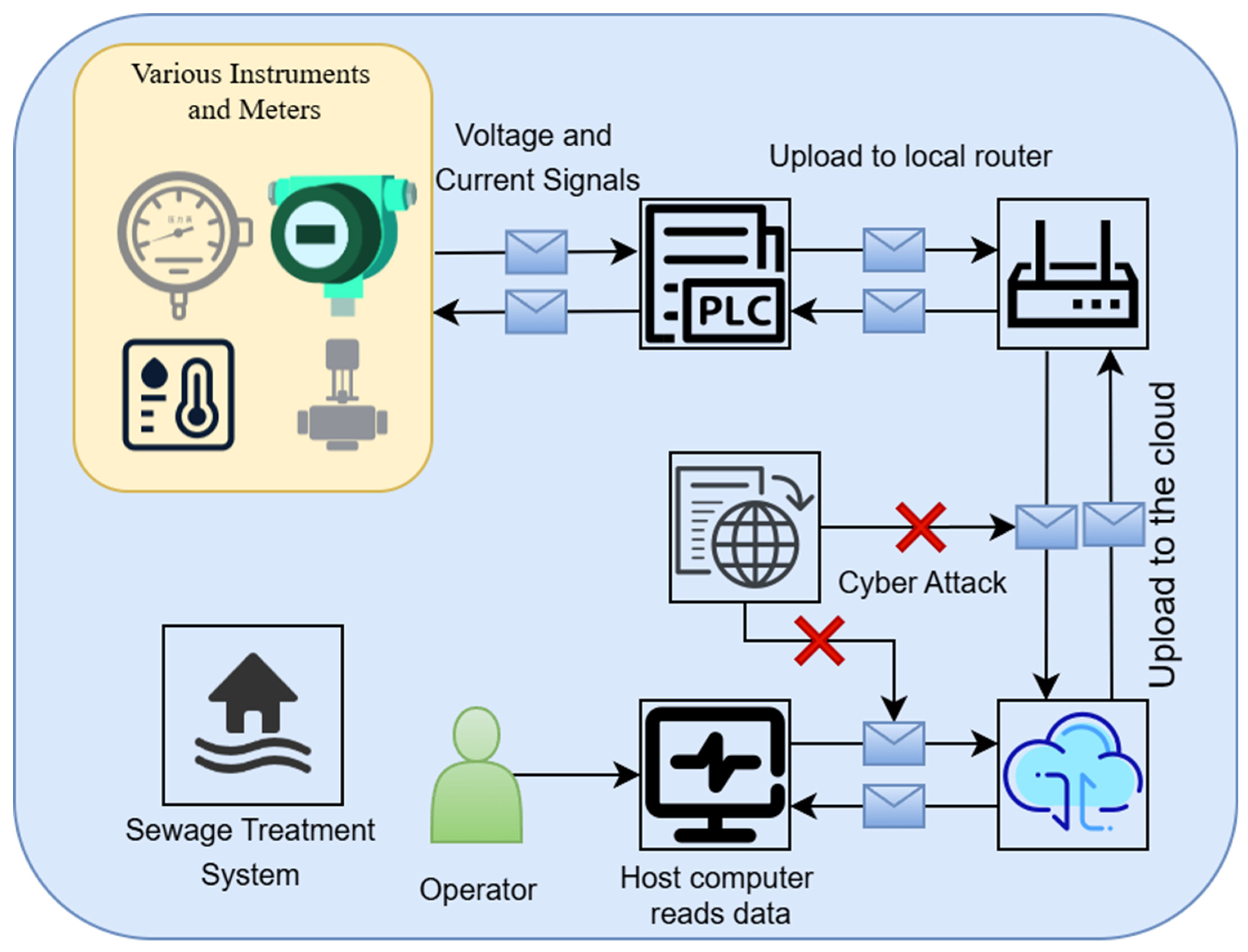
Figure 1. Signal Flow Diagram of the Wastewater Treatment System.
Water 17 02842 g001
Figure 2. Water Treatment System Anomaly Detection Model.
Water 17 02842 g002
Figure 3. Flowchart of VAE-based anomaly detection.
Water 17 02842 g003
Figure 4. Flowchart of LSTM-based anomaly detection.
Water 17 02842 g004
Figure 5. Two-stage hybrid VAE–LSTM anomaly detection framework with dynamic thresholding and weighted scoring.
Water 17 02842 g005
Figure 6. Changes in FIT101 Sensor under Attack in the SWaT Water Treatment System.
Water 17 02842 g006
Figure 7. Changes in MV101 Sensor under Attack in the SWaT Water Treatment System.
Water 17 02842 g007
Figure 8. Changes in the LT101 Sensor under Attack in the WADI Water Treatment System.
Water 17 02842 g008
Figure 9. Changes in MV101 Sensor under Attack in the WADI Water Treatment System.
Water 17 02842 g009
Figure 10. Variation in the Objective Function Value with Iteration Number.
Water 17 02842 g010
Figure 11. Probability Density and Reconstruction Error Distribution after Processing Normal Data.
Water 17 02842 g011
Figure 12. Algorithm Performance Comparison in SWAT.
Water 17 02842 g012
Figure 13. Comparison of Algorithm Training and Detection Time.
Water 17 02842 g013
Figure 14. Algorithm Performance Comparison in WADI.
Water 17 02842 g014
Table 1. Process Overview of the SWaT Water Treatment System.
Water Treatment StepStep DescriptionMonitored Sensor IDMonitored Actuator ID
Step 1Raw Water IntakeFIT101 LIT101MV101 P101 P102
Step 2Chemical DosingAIT201 AIT202 AIT203 FIT201MV201 P201 P202 P203 P204 P205 P206
Step 3Ultrafiltration (UF) System FiltrationDPIT301 FIT301 LIT301MV301 MV302 MV303 MV304 P301 P302
Step 4UV Disinfection and DechlorinationAIT401 AIT402 LIT401P401 P402 P403 P404 UV401
Step 5Feed to Reverse Osmosis (RO) SystemAIT501 AIT502 AIT503 AIT504 FIT501 FIT502 FIT503 FIT504 PIT501 PIT502 PIT503P501 P502
Step 6Backwash Cleaning of UFFIT601P601 P602 P603
Table 2. Process Overview of the WADI Water Treatment System.
Water Treatment StepStep DescriptionMonitored Sensor IDMonitored Actuator ID
Step 1Wastewater enters the main network
1-T001 1-T002
1-LT-001 1-FS-0011-MV-001 1-MV-005 1-P-005
Step 2AStorage in elevated tanks
2-T-001 2-T-002
2-LT-001 2-PIT-001 2-FS-001 2-FS-0022-MV-001 2-MV-002 2-MV-003 2-MV-004 2-MV-005 2-MV-006 2-P-003 2-P-004
Step 2BResidential water storage
2-T101 2-T201 2-T301 2-T401 2-T501 2-T601
2-FQ-101 2-FQ-201 2-FQ-301 2-FQ-401 2-FQ-501 2-FQ-601 2-PIT-0022-MV-101 2-MV-201 2-MV-301 2-MV-401 2-MV-501 2-MV-601 2-MCV-101 2-MCV-201 2-MCV-301 2-MCV-401 2-MCV-501 2-MCV-601
Step 3Water recirculation to the main network
3-T-002
3-LT-001 3-FS-001 3-FS-0023-MV-002 3-P-003 3-P-004
Table 3. SWaT and WADI Water Treatment System Datasets.
DatasetNumber of Training SamplesNumber of Testing SamplesNumber of Available Signal Groups
SWaT December 2015495,000449,91951
WaDi October 20171,209,600172,806123
Table 4. Description and Range of Hyperparameters for Bayesian Optimization.
Parameter NameDescriptionParameter Setting
vae_latent_dimVAE latent dimensionInteger, range [2, 20]
vae_hidden_dimVAE hidden layer dimensionInteger, range [10, 100]
kl_weightKL divergence weightReal, range [0.1, 1.0]
lstm_layersLSTM number of layersInteger, range [1, 3]
lstm_hiddenLSTM hidden unitsInteger, range [32, 128]
lstm_biBidirectional LSTMBoolean, False or True
lstm_dropoutLSTM dropout rateReal, range [0.0, 0.5]
aVAE reconstruction loss weightReal, range [0.0, 0.9]
cLSTM reconstruction loss weightReal, range [0.0, 0.9]
Table 5. Optimal Hyperparameters.
HyperparameterV_Latent_DimVae_Hidden_DimKl_WeightLstm_Layers
Optimal Value2301.02
lstm_hiddenlstm_bilstm_dropoutac
64False0.3550.05990.037
Table 6. Hyperparameters of Isolation Forest.
Parameter NameDescriptionParameter Setting
n_estimatorsNumber of trees in the Isolation Forest100
max_samplesNumber of samples randomly drawn to build each treeauto
contaminationProportion of anomalies in the dataset0.1
max_featuresProportion of features randomly selected to build each tree1.0
bootstrapWhether to use bootstrap sampling when building each treeFalse
random_stateRandom seed42
Table 7. Hyperparameters of One-Class SVM.
Parameter NameDescriptionParameter Setting
kernelType of kernel functionrbf
degreeDegree for the polynomial kernel function3
nuUpper bound on the fraction of support vectors and lower bound on training error0.05
tolError tolerance for stopping criterion0.001
cache_sizeSize of the kernel computation cache200
Disclaimer/Publisher’s Note: The statements, opinions and data contained in all publications are solely those of the individual author(s) and contributor(s) and not of MDPI and/or the editor(s). MDPI and/or the editor(s) disclaim responsibility for any injury to people or property resulting from any ideas, methods, instructions or products referred to in the content.