Article

Risk Assessment of Debris Flow in the Kashgar-to-Khunjerab Section of the China–Pakistan Economic Corridor

Institute of Geological Hazards Prevention, Gansu Academy of Sciences, Lanzhou 730099, China
*
Author to whom correspondence should be addressed.
Water 2025, 17(19), 2841; https://doi.org/10.3390/w17192841
Submission received: 19 June 2025 / Revised: 22 August 2025 / Accepted: 4 September 2025 / Published: 28 September 2025
(This article belongs to the Section Hydrology)

Abstract

The risk of debris flow comprehensively reflects both the natural and social attributes of debris flow disasters, composed of the hazard of debris flow and the vulnerability of the bearing body. The geological environment of the Kashgar-to-Khunjerab section of the China–Pakistan Economic Corridor is complex, with widespread debris flow disasters, strong activity, and severe hazards, posing a significant threat to corridor construction and public safety. Therefore, conducting debris flow risk assessments in the Kashgar-to-Khunjerab section of the China–Pakistan Economic Corridor has great significance for disaster prevention and control. Based on field investigation data of debris flows, this study evaluates the hazard of debris flows in the study area through the frequency ratio and frequency ratio–logistic regression coupled models. The vulnerability of debris flows was evaluated through a contribution weight model. Based on the assessment results of hazard and vulnerability, a risk assessment model was utilized to explore the risk situation of debris flow disasters in the Kashgar-to-Khunjerab section of the China–Pakistan Economic Corridor. The results show that the frequency ratio–logistic regression coupled model (AUC = 0.867) is more suitable for debris flow disasters hazard assessment. The area of medium hazard zones and above accounts for 68.6% of the total area. The vulnerability in the study area is generally concentrated in the township regions along the Kashgar-to-Khunjerab section of the China–Pakistan Highway. The proportion of medium and above vulnerability zones areas reaches 55.6%. The risk levels of the study area generally radiate outward from the Kashgar-to-Khunjerab section of the China–Pakistan Highway, exhibiting a decreasing trend of from high to low. The distribution areas of different risk zones initially increase and then decrease with the rise in risk levels, and the area of medium risk zones and above accounts for 50.8% of the total area. Approximately 91.7% of debris flow disaster points are located in high and very high risk zones. This indicates that the study area has a high level of risk. The study results can provide a scientific basis for planning debris flow disasters prevention and mitigation measures, and the proposed assessment methods can also serve as a reference and guidance for debris flow risk assessment in the study area and other regions.

1. Introduction

Worldwide, mountainous geological hazards are one of the most common natural disasters [1], and debris flows are among the most widespread and destructive geological hazards in mountainous regions [2]. In recent years, the increased frequency of earthquakes and extreme weather events has significantly raised the occurrence and scale of debris flow activity [3]. Meanwhile, with the continuous development of socioeconomics and the expansion of human activities in mountainous areas, infrastructure construction has accelerated, further exacerbating the adverse impacts of debris flows. These disasters pose serious threats to human safety and property. The China–Pakistan Economic Corridor is one of the six major economic corridors identified as part of China’s Belt and Road Initiative. It connects the “Maritime Silk Road” in the south with the “Silk Road Economic Belt” in the north, making it a pioneer zone for the Belt and Road development. It is a critical economic route that encompasses transportation, energy, communications, agriculture, and hydropower, holding significant strategic importance [4]. The China–Pakistan Economic Corridor is located in the southwest of Xinjiang, eastern Pamir Plateau, and western section of the Kunlun Mountains, where the geological environment is highly complex and variable. Under the influence of a warming and humidifying climate, debris flow disasters in this area have become more frequent, expanding the disaster risk, severely threatening road transportation, and posing a significant challenge to the sustainable socioeconomic development [5,6,7]. Therefore, conducting research on regional debris flow risk has great significance for disaster mitigation and risk control in the area.
Risk is defined as the expected degree of loss resulting from a potentially hazardous event with a given intensity and frequency [8]. It involves three key components: the hazard-forming environment, triggering factors, and elements at risk [9]. In the context of debris flow disasters, the regional risk assessment is a more suitable quantitative assessment method, which can systematically predicts and quantifies the probability of debris flow occurrence and its potential impacts, including casualties, property damage, and economic losses [10,11,12,13,14,15]. Scientific and effective risk assessment for debris flows can not only guide the precise implementation of disaster relief measures but also provide a theoretical basis for disaster prevention planning [16,17,18]. Based on this, many researchers have carried out studies on debris flow risk assessment by various methods. The core components of debris flow risk assessment are hazard assessment and vulnerability assessment [7]. Debris flow hazard refers to the likelihood of debris flow occurrence in a specific region and the extent of damage it could cause to human life, property, and the ecological environment [19]. The influencing factors are related to topography, geological structure, vegetation cover, land use, and climatic and hydrological condition, such as elevation, elevation difference, slope, aspect, lithology, distance to faults, vegetation cover, land use, annual mean precipitation, and distance to rivers [20,21,22]. For hazard assessment, many scholars have used qualitative and quantitative analysis methods for debris flow hazard assessment [23]. The qualitative methods, such as expert scoring and analytic hierarchy process, tend to be influenced by human factors and lack objectivity [24,25,26,27]. While quantitative methods extract and analyze a large amount of data to determine the weights of assessment indicators, they reduce the influence of expert subjectivity. Sujatha et al. [28] employed the Analytical Network Process (ANP) to generate a debris flow susceptibility map by integrating key factors including material availability, peak flow, slope gradient, land use and land cover, and distance to streams, etc. Xu et al. [29] employed a method combining GIS technology with the Information Value to evaluate debris flow hazard in Sichuan Province, selecting seven environmental factors, such as elevation, slope, aspect, flow accumulation, vegetation coverage, soil type, and land use type. Zhou et al. [7] utilized remote sensing and GIS technologies to select 17 influencing factors, including area, average slope, lithology, net primary productivity (NPP), mean annual precipitation, landslide density, drainage density, and fault density, etc., and applied machine learning algorithms to develop a debris flow hazard assessment model for the Bailong River basin. Through research, it has been found that the above-mentioned single assessment methods have certain limitations and cannot fully reflect the complex nonlinear relationships between debris flow and the indicator factors. Based on this, after conducting a comparative analysis of the advantages of various methods, this study selected the frequency ratio and the frequency ratio–logistic regression coupled model to assess the debris flow hazard in study area. The advantage of the coupled model lies in its ability to not only consider the contribution rates of different factor classes to debris flow occurrence, but also to incorporate the relative importance of each influencing factor. This coupled model enhances the overall accuracy and reliability of the hazard assessment [30].
Vulnerability is a complex concept involving numerous factors, originating from the study of natural disasters, used to evaluate human socioeconomic systems as elements at risk. It is a component of disaster risk analysis and reflects the strength of the disaster-bearing capacity, guiding disaster prevention and mitigation efforts to ensure the safety of lives and property [31,32]. For vulnerability assessment, scholars have proposed many practical and effective assessment methods. Li et al. [33] introduced a comprehensive approach combining Bayesian network models and spatial analysis to predict the impacts of natural disaster vulnerability. Chen et al. [34] summarized the conceptual framework of vulnerability based on collected literature. Formulation and components of vulnerability, exposure, sensitivity, and adaptive capacity were analyzed in depth under different research contexts. Shu et al. [5] considering the exposure (debris flow catchment area, density of debris flow disaster points), sensitivity (casualties and property losses), and recovery capacity (total local fiscal revenue, occupational structure of residents) of disaster-bearing body, the vulnerability values of various townships in the Wudu District were calculated by the DEA model and C-D function, and then, vulnerability grading map of villages and towns in the study area was obtained. Ding et al. [35] adopted the Contribution Weighting Superposition method to construct a regional debris flow vulnerability assessment model and system. The model includes 13 indicator factors, covering population, economy, road density, and other related aspects. Cui et al. [36] utilized factor analysis to establish a vulnerability index system for roads in earthquake-affected areas and obtained a vulnerability zoning map for Provincial Road 303 in Sichuan Province. Gao et al. [37] employed the Contributing Weight Superposition model to establish a quantitative method for geological disaster vulnerability assessment in the Qiaojia seismic area in Southwestern China. In conclusion, most current studies focus on exposed buildings, infrastructure, and lifelines, while lacking research on the multidimensional characteristics of vulnerability. The Contribution Weighting Superposition method offers a new approach to vulnerability assessment; its advantage lies in the fact that the predictive weight of each indicator is entirely determined by objective data, thus overcoming the subjective biases often present in manual scoring [7]. Therefore, this paper applies this method to evaluate the vulnerability of debris flows in the study area.
The primary goal of debris flow risk assessment is to systematically evaluate the hazard and potential impacts of debris flows, identify high-risk areas, and reduce the probability and losses of debris flow disasters. This is critical for the prevention and mitigation of mountain hazards [38]. In this study, the section from Kashgar to Khunjerab along the China–Pakistan Economic Corridor is selected as the study area. Based on field study data of debris flow disasters, key indicators for hazard and vulnerability assessment are chosen. Various models are used to explore the spatial distribution characteristics of debris flow hazard, vulnerability, and risk, the debris flow assessment specifically focuses on the road corridor and its adjacent areas. The results not only assist in further enriching and improving the theoretical framework of debris flow assessment, but also hold significant practical significance, providing a solid theoretical foundation and practical guidance for sustainable regional development.

2. Study Area

Kashgar-to-Khunjerab section of the China–Pakistan Economic Corridor coincides with the southwest end of the National Highway 314. It is an important national defense highway connecting China and Pakistan, also known as the “China–Pakistan Friendship Highway”. In the administrative division, this area is divided into two administrative regions: Kashgar and Kizilesukeerkezi, which starts from Kashgar of Xinjiang in the east and enters Pakistan through Aoyitake, Bulunkou, Tashikuergan, Dabudaer, and Khunjerab, crossing river terraces or valleys between snow-covered mountains [6]. Rainfall is unevenly distributed in the study area, mainly concentrated from May to September each year. Intense rainfall provides favorable conditions for the formation of debris flow [39]. In addition, the study area is located in an area with harsh natural conditions such as geology, topography, climate, and hydrology, with frequent occurrences of multiple geological disasters such as debris flows. According to hydrodynamic triggering condition analysis, the study area not only exhibits rainfall-triggered debris flows, but also contains a significant number of glacier-triggered and hybrid rainfall–glacier-triggered debris flows [40], which seriously threaten road travel and safety. After remote-sensing interpretation and field investigation, it was found that there were 511 debris flow channels, which are distributed mainly along the Kashgar-to-Khunjerab section of the China–Pakistan Highway (Figure 1), and the distribution density of various types of debris flows along the China–Pakistan Highway reaches 1.2 per kilometer [6].

3. Data and Methods

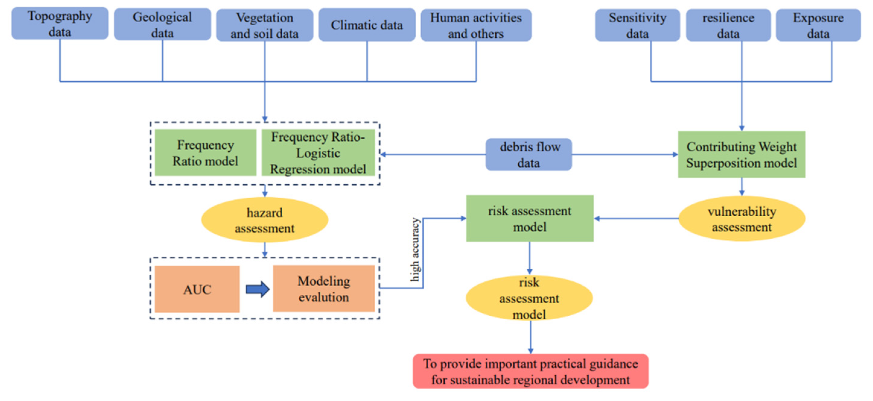
This study selects 12 hazard assessment indicators from five aspects—topography and geomorphology, geological structure, vegetation and soil, climatic, and human activities—to establish a hazard assessment system. The frequency ratio model and the frequency ratio–logistic regression coupled model are used to evaluate the debris flow hazard in the study area, and the models are evaluated using the AUC value of the ROC curve to determine the optimal model. For vulnerability, six assessment indicators are selected from the aspects of exposure, sensitivity, and resilience to establish a vulnerability assessment system. The Contributing Weight Superposition model is applied to evaluate the debris flow vulnerability in the study area. Based on the hazard and vulnerability assessment results, a risk assessment model is used to obtain the debris flow risk assessment results for the study area. The specific process is shown in Figure 2.

3.1. Data

3.1.1. Debris Flow Hazard Data

The occurrence of debris flow needs to fulfill three key conditions, steep topography, sufficient material sources, and heavy rainfall. Therefore, this study synthesizes various factors; historical debris flow disasters characteristics, unique topography, geomorphology, environmental conditions of the study area, literature and expert consultation, field survey, and the assessment indicators related to topography and geology, vegetation and soil, temperature and precipitation, distance to rivers, and land use were selected. We employed the Variance Inflation Factor (VIF) to test for multicollinearity among these indicators, retaining only the 12 indicators with VIF < 10 [41,42], establishing a debris flow disasters hazard assessment system in the study area. The specific data sources for these assessment indicators are shown in Table 1.
(1)
Topographic and geomorphological
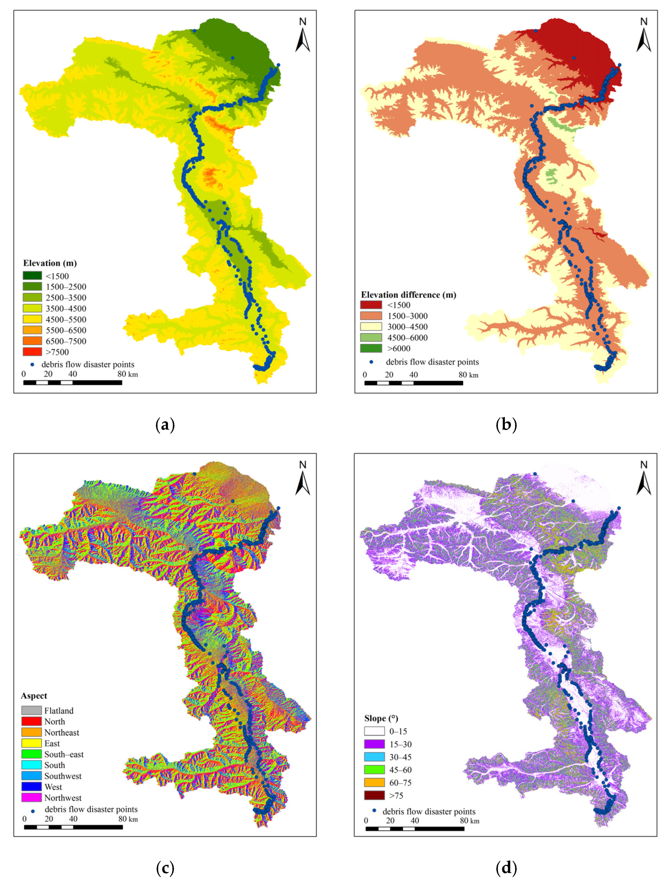
The topographic and geomorphological data mainly include elevation, relative elevation difference, slope, and slope direction, among which the elevation directly reflects variations in topographic undulation, gullies, vegetation types, soil types, and precipitation in the study area. Therefore, elevation has a significant impact on debris flow. In this study, the elevation of the study area is classified into eight classes: 0–1500 m, 1500–2500 m, 2500–3500 m, 3500–4500 m, 4500–5500 m, 5500–6500 m, 6500–7500 m, >7500 m, as shown in Figure 3a.
The elevation difference mainly controls the development of surface vegetation and bedrock exposure. The study area is located in the southwestern part of the Xinjiang Uighur Autonomous Region, the eastern part of Pamir Plateau, and the western part of Kunlun Mountain Range, and the road crosses the river terrace or canyon area between high mountains (snow mountains). The mountains are steep, the rivers are strongly undercut, and the alpine canyon terrain is very developed, which provides dynamic conditions for debris flow initiation. Based on the elevation data of the study area, the relative elevation difference is divided into five classes: 0–1500 m, 1500–3000 m, 3000–3500 m, 3500 m–6000 m, >6000 m, as shown in Figure 3b.
Aspect has a significant influence on the formation, distribution, and activity intensity of debris flow. Aspect controls the distribution pattern of microclimate and water–heat ratio on mountain slopes. The difference in topographic slope between mountains and river valleys affects the amount of snow and ice accumulation, melting, and rainfall, as well as the growth of vegetation and the degree of rock weathering. In the shaded slope zone, snow and ice storage conditions are favorable, the snow line is lower than the sunny slope, glaciers are more developed than the sunny slope, the altitude of glacial terminus is low, the glacier is relatively stable, so the debris flow formation solid material source and water source conditions are poor, debris flow activity is not obvious. On the sunny slope, there is more sunlight intensity and radiation, the ice and snow melt quickly, the rock weathering is fast and high, the rock and soil structure is looser, and the debris flow material source and water source are more abundant, which causes the phenomenon that the debris flow on the sunny slope is generally more developed than that on the shady slope, as shown in Figure 3c.
The slope is a critical factor influencing the development of debris flows. The slope directly reflects the steepness change in the terrain, which affects the stability of loose material sources, the flow rate of surface runoff, and indirectly affects the development of debris flow. It has some influence on the mechanism of slope deformation. The slope was obtained from elevation data by slope function extraction. In this study, slope was classified into five classes: 0–15°, 15–30°, 30–45°, 45–60°, 60–75°, and >75°, as shown in Figure 3d.
(2)
Geological structure
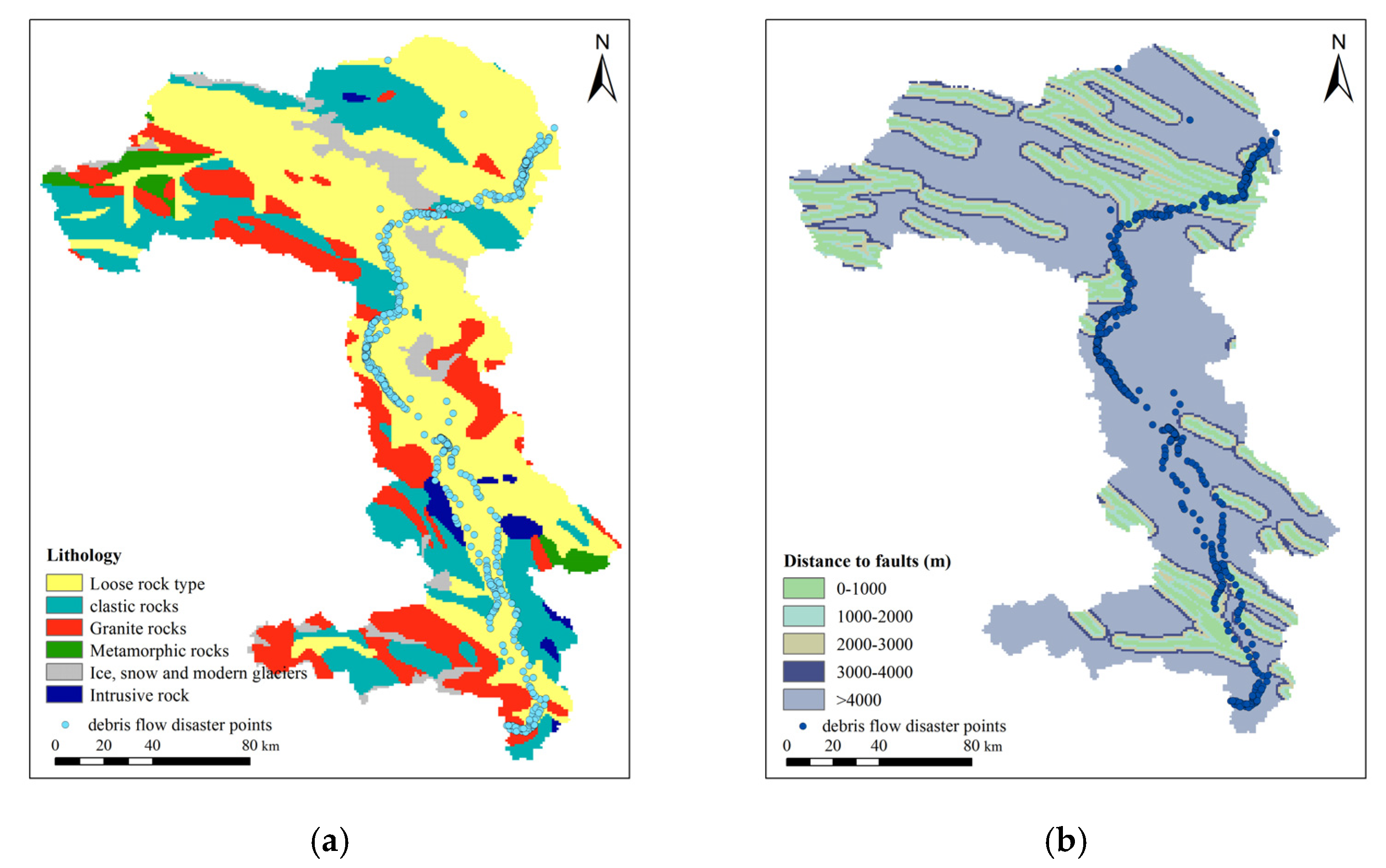
In lithology, stratigraphic rocks are one of the main substances that form the source of debris flow. The lithology of different types of rocks has different physicochemical properties and weathering levels [43]. The properties of stratigraphic rock masses vary, resulting in differences in weathering degree, distribution of joints and fissures, rock strength, and water content. The rocks have been affected by weathering for a long time in the study area, and the broken rocks often converge into the channel, which provides favorable conditions for the recharge of loose solid material sources. Based on the actual geological data and field investigation, the stratigraphic lithology of the study area is divided into six categories: loose rock, clastic rock, granite, metamorphic rock, ice and modern glaciers, and intrusive rock, as shown in Figure 4a.
The formation of debris flows is generally inextricably linked to fault structures, especially in the cross-compound parts of regional fault structures, where fault movements make rocks broken and less stable, and easily form structural conditions favorable for the development of debris flows. Therefore, this study chooses the distance from fault to analyze the risk of debris flow. Based on the actual situation of the fault distribution in the study area, a buffer zone of 1 km from the faults is analyzed and divided into five categories: 0–l000 m, l000–2000 m, 2000–3000 m, 3000–4000 m, and >4000 m, as shown in Figure 4b.
(3)
Vegetation and soil
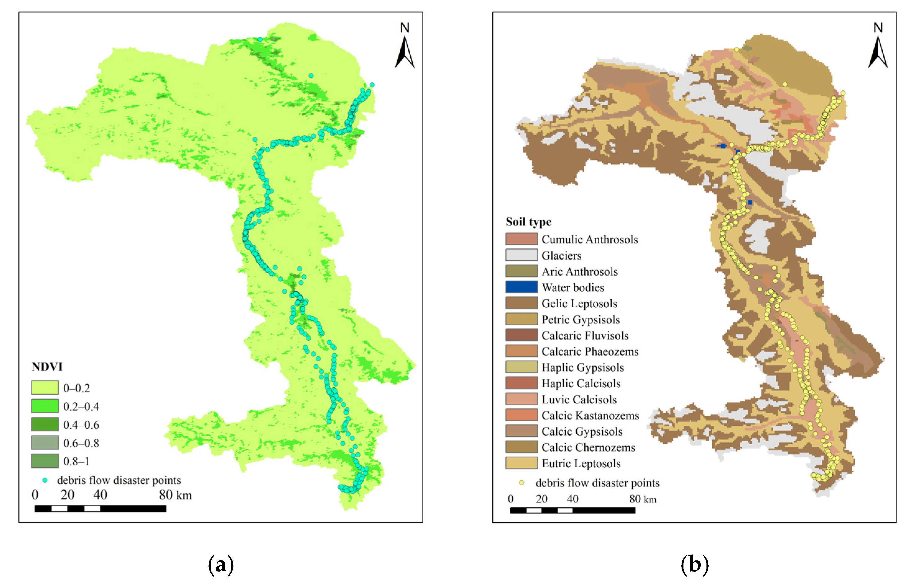
Vegetation is one of the key factors influencing the development of debris flows, mainly reflected in the fact that the rhizome of vegetation has a certain root reinforcement effect on the soil; this helps to reduce the flow velocity and infiltration rate of water on slopes, enhance the shear strength of the geotechnical body and the degree of soil consolidation, and ultimately prevent soil erosion [10]. The normalized Difference Vegetation Index (NDVI) can effectively reflect the vegetation growth status and vegetation cover. Therefore, NDVI is used as an indicator to evaluate the impact of vegetation cover on debris flow disasters and to judge the distribution of debris flow disaster. Based on NDVI data, this study classifies NDVI into five categories: 0–0.2, 0.2–0.4, 0.4–0.6, 0.6–0.8, and 0.8–1, as shown in Figure 5a.
Soil type has a large impact on surface infiltration and erosion resistance. Different soil types have different particle sizes, different degrees of compactness, and different permeability. The more compact the soil structure, the better its water retention, the less soil erosion occurs, and the fewer loose materials are carried by the water flow, resulting in less material source replenishment for debris flow formation; on the contrary, loose soil structures allow rainwater to erode the surface, increasing material source replenishment for debris flow. Therefore, the soil plays a crucial role in the formation of loose surface materials. Through field surveys and remote sensing data analysis, the soil types in the study area are classified into 15 categories; specific classification is shown in Figure 5b.
(4)
Climatic conditions
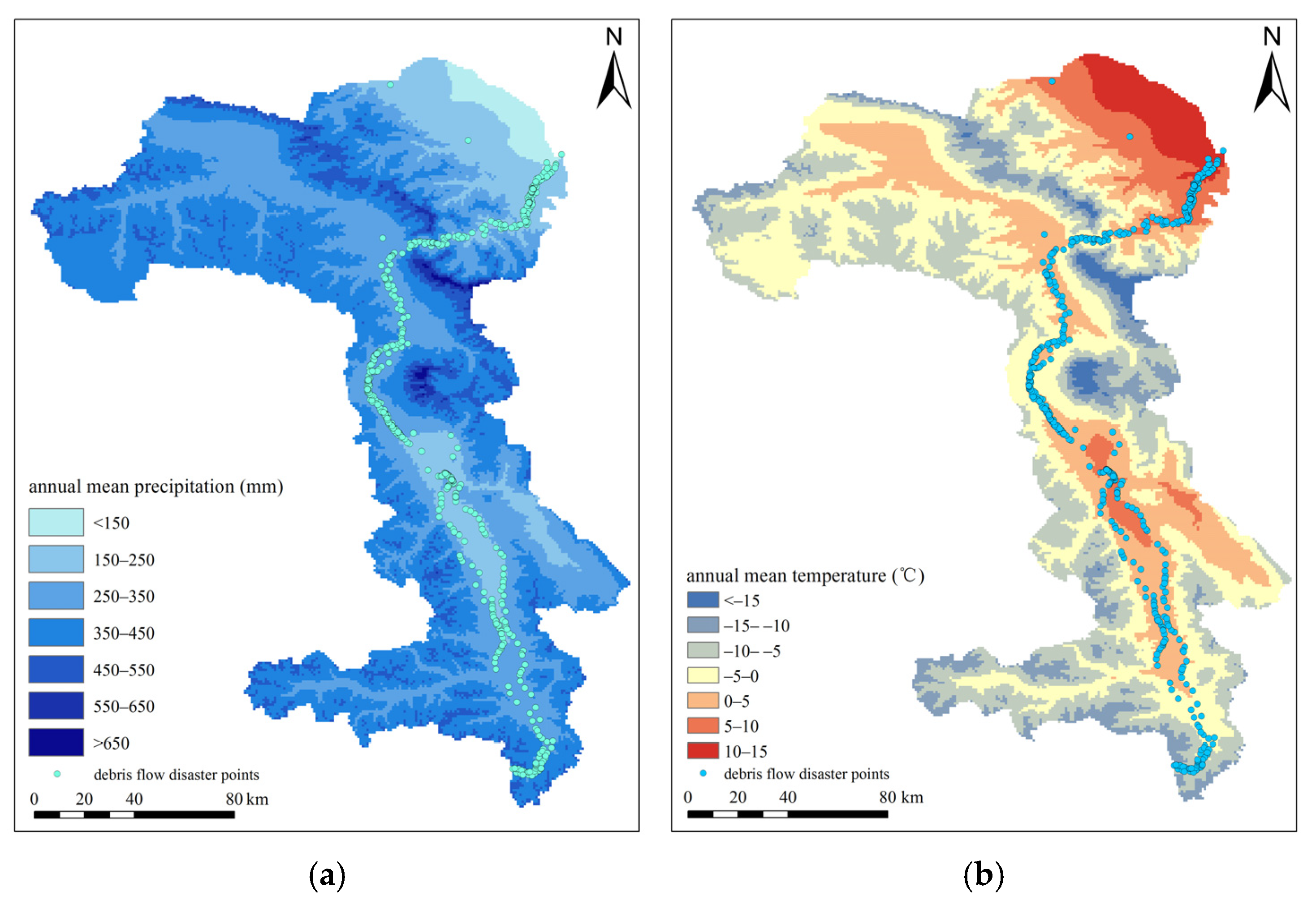
Precipitation is the main factor that induces debris flows [44]. As precipitation increases, the pore water pressure within loose rock and soil on slopes rises, reducing shear strength, which leads to landslides and collapses, providing abundant loose solid materials for the formation of debris flows. In addition, heavy precipitation can generate channel floods, and the strong currents generate strong impact force and a powerful scouring and transporting effect on materials at the foot of slopes and in riverbeds, ultimately leading the solid materials to be mobilized by the floodwaters, forming debris flows. Approximately 70% of the annual precipitation in the study area occurs between June and August, and short-duration, intense convective weather events frequently occur [45]. These climatic conditions are highly conducive to the initiation of debris flow disasters. Therefore, in this study, annual mean precipitation from 1960 to 2020 in the study area was used as an indicator to evaluate the impact of precipitation on debris flow disasters. The maximum annual mean precipitation is 763.35 mm, the minimum annual mean precipitation is 113.45 mm, and the annual mean precipitation is 359.56 mm. Based on the maximum and minimum annual mean precipitation values, the annual mean precipitation in the study area is classified into seven categories; specific classification is shown in Figure 6a.
The China–Pakistan Economic Corridor is located in mountainous areas with a complex geological environment, and glaciers are present in the valleys. In summer, the high temperatures in the study area accelerate glacier melting, generating substantial meltwater that may trigger glacial meltwater debris flow disasters. For instance, at 15:00 on 22 July 2021, during a debris flow survey in Bulunkou Township, Akto County, scientific investigators observed a debris flow event triggered by glacial meltwater. Therefore, temperature is another important factor influencing debris flow disasters in the study area. This study selected the annual mean temperature from 1960 to 2020 to reflect the climate conditions of the study area. The maximum annual mean temperature is 12.08 °C, the minimum annual mean temperature is −28.67 °C, and the annual mean temperature is −3.05 °C. Based on the maximum and minimum annual mean temperature values, the annual mean temperature is classified into seven categories; specific classification is shown in Figure 6b.
(5)
Human activities and others
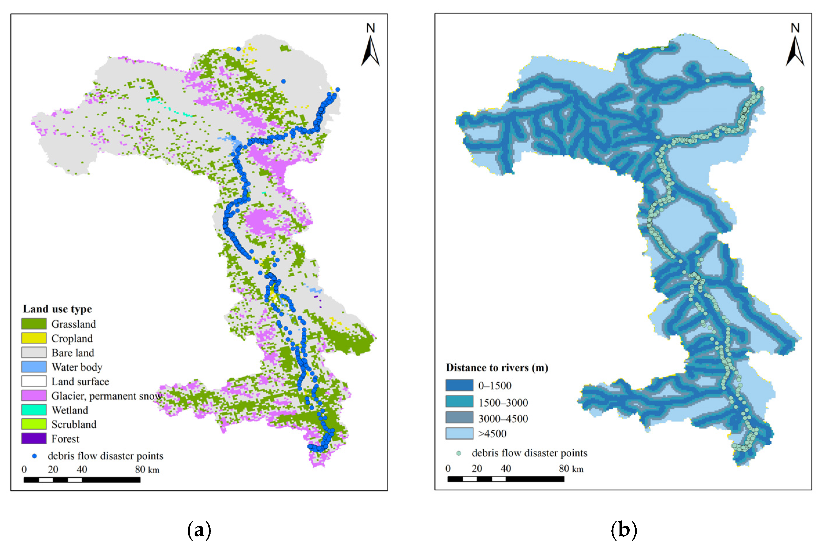
Land use types influence the occurrence of debris flows by altering surface vegetation cover and hydrological conditions. Different land use types exert varying impacts on the formation and development of debris flows, with activities that damage the ecological environment exacerbating the formation and occurrence of debris flows. Through field surveys and remote sensing data analysis, the land use types in the study area are classified into nine types; specific classification is shown in Figure 7a.
The debris flow often occurs in mountainous gullies, which often block rivers, and river gullies also provide flow channels for debris flow, extending their flow distance and increasing their scale. The buffer zones of rivers in the study area are classified into five categories, which are 0–1000 m, 1000–2000 m, 2000–3000 m, 3000–4000 m, and >4000 m, as shown in Figure 7b.

3.1.2. Debris Flow Vulnerability Data

The vulnerability assessment of debris flows consists of three components: exposure, sensitivity, and resilience [5]. The exposure index is measured by the relative spatial location of debris flows and the density of debris flow disaster points. The sensitivity index is represented by population density and road density in terms of hazard losses. Resilience is relatively abstract and difficult to quantify. It is represented by GDP and the distance from towns. Specific details and the source of data are shown in Table 2.
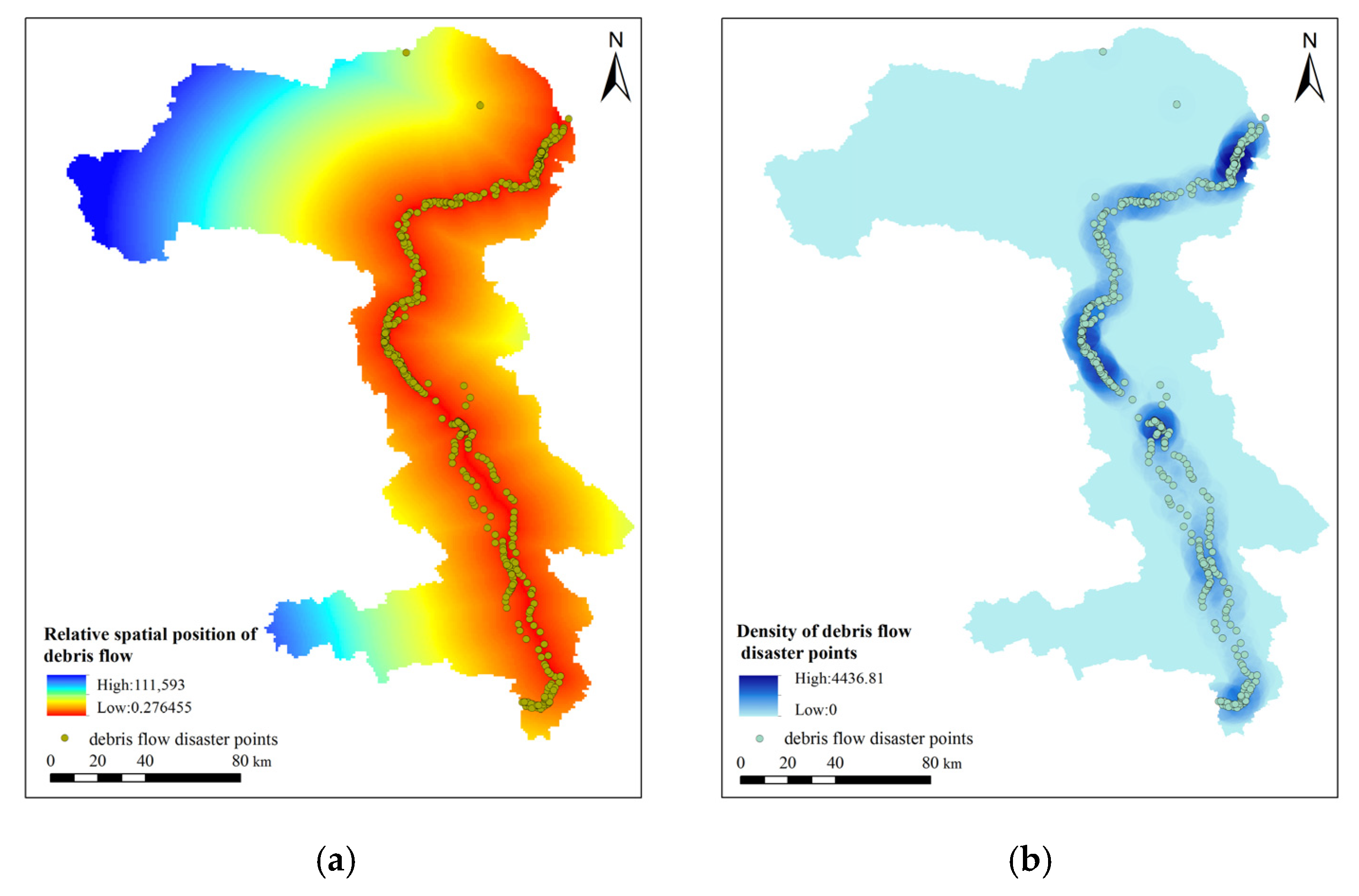
Exposure reflects the degree of external disturbance and threat. Under the same debris flow conditions, the higher the exposure of the area, the greater the absolute value of the damage caused by the disaster. In this study, exposure is measured by the density of debris flow disasters and the relative spatial location of debris flow. The density of debris flow disaster points reflect the spatial distribution characteristics of debris flow in the area, while relative spatial location of debris flow directly determines the degree of damage suffered by debris flow in the area. Both are the basic factors influencing the vulnerability of debris flows, as shown in Figure 8.
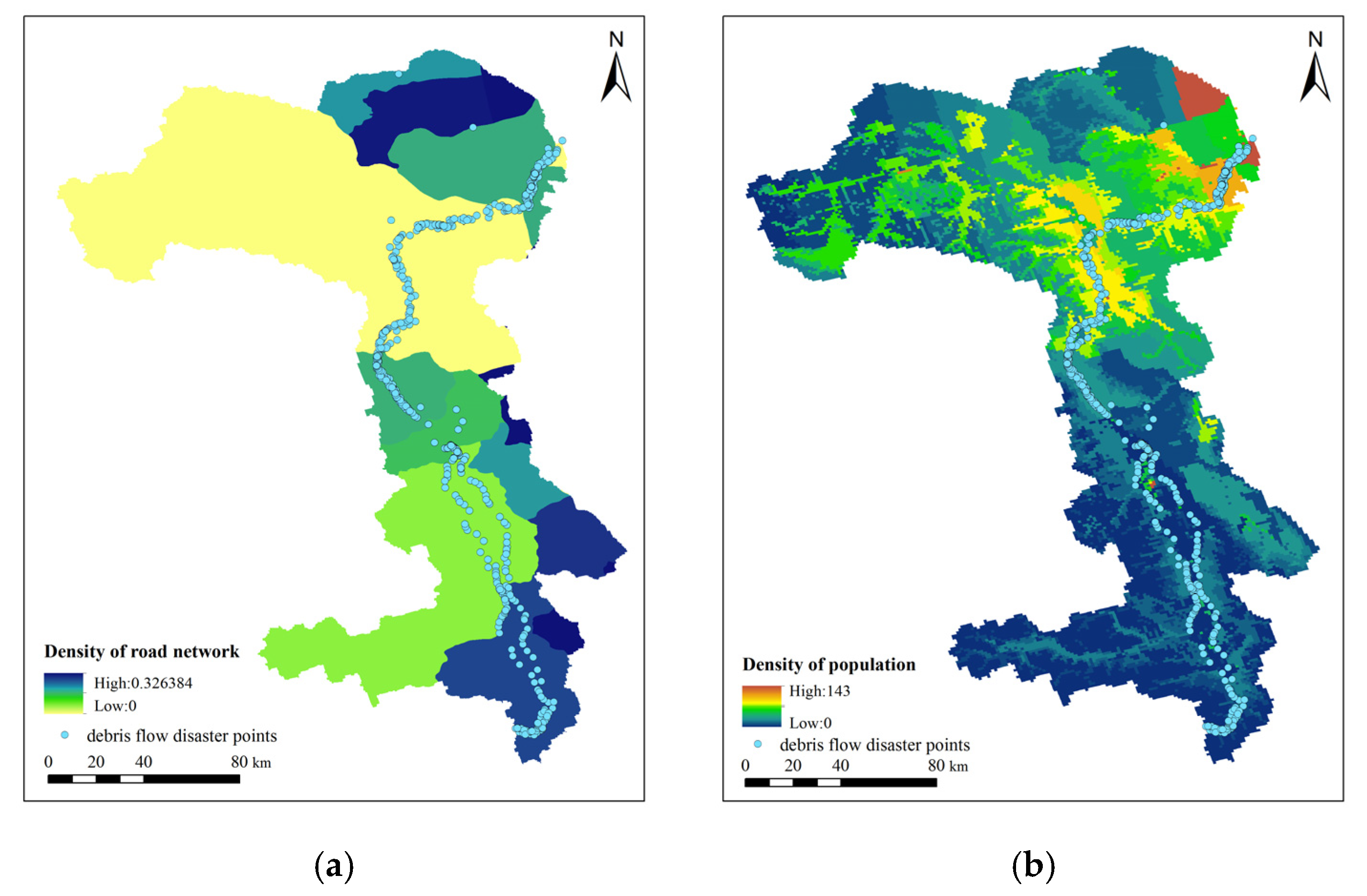
Sensitivity reflects the potential changes that disturbances may cause in socio-ecological systems. In this study, sensitivity is measured by population density and road density. Population density reflects the characteristics of regional population distribution; the lower the population density, the smaller the impact caused by debris flow disasters. Road construction is a prerequisite for economic development. Road accessibility is crucial for debris flow disaster prevention and mitigation. Higher road density indicates stronger capacity to cope with debris flow disasters. Additionally, road density is also important for social security in emergency situations, as shown in Figure 9.
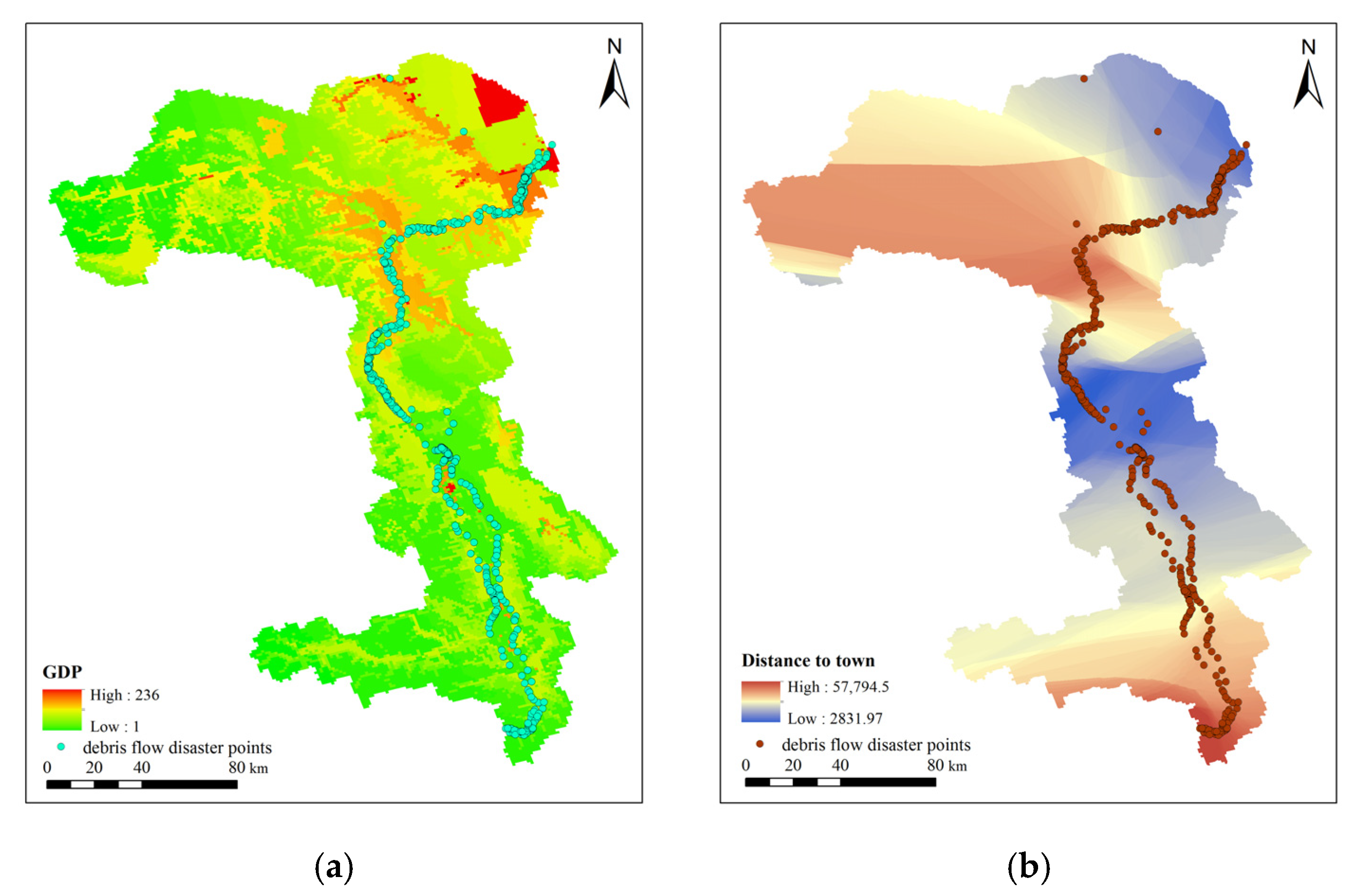
Resilience reflects the system’s ability to recover from the adverse effects caused by disturbances. In this study, resilience is measured by GDP and the distance to town. GDP mainly reflects the economic strength of a region. The larger the GDP value, the faster the recovery from the damage caused by the debris flow disasters. The closer the distance to a town, the quicker the rescue and recovery after the destruction caused by debris flows, as shown in Figure 10.

3.2. Methods

3.2.1. Hazard Assessment Method

(1)
Frequency Ratio Model
The frequency ratio method is widely applied in geological hazard assessment; its principle involves analyzing the spatial relationships between debris flow distribution and influencing factors [30,42]. This method integrates spatial data with analytical models to quantitatively evaluate the hazard of debris flow disasters. The frequency ratio model has been effectively applied in previous geological disaster assessments and factor contribution calculations. Its formula is as follows:
F R i j = L N i j L N N i j N 100 %
H = F R i j
In the formula, FRij is the frequency ratio of the i factor and j grade; LNij is the i factor and j grade debris flow pixel; ∑LN is the study area debris flow pixel; Nij is the i factor and j grade area pixel; ∑N is the total study area pixel; H is the debris flow susceptibility index.
(2)
Frequency Ratio–Logistic Regression Model
In order to take into account the advantages of frequency ratio and logistic regression models, the coupled model was invoked to evaluate the debris flow disasters in this study. The model not only comprehensively considers the effects of different intervals of influencing factors on debris flow disasters but also analyzes the contribution of each factor at different levels and its importance to the occurrence of debris flows. In order to reduce the influence of different amplitudes, the frequency ratio is normalized between [0, 1] [46], and the specific calculation formula is as follows:
L o g i t H = b 0 + b 1 y i + b 2 y i + b n y i
In the formula, LogitH is the probability function of debris flow occurrence, b0 is a constant term, b1, b2, …, bn are the regression coefficients of the normalized values, which belong to the frequency ratio of each factor, and yi denotes the normalized value of the frequency ratio of each factor.
(3)
ROC Curve
In this study, ROC (Receiver Operating Characteristic Curve) curve and model plausibility testing are used to choose more suitable hazard assessment method. The AUC is usually used to assess the reliability of the model, representing the area under the ROC curve. The criteria are as follows: when the AUC < 0.5, the prediction results are not credible; when the AUC = 0.5, the results are random; when AUC is between 0.5 and 0.7, the accuracy is low; when AUC is between 0.7 and 0.9, the accuracy is high; and when the AUC > 0.9, the accuracy is extremely high [44]. In this study, there were 511 debris flow disaster points in the study area, which were taken as debris flow disaster sample points with a value of “1”, and 511 points were randomly taken as non-debris flow disaster sample points with a value of “0” in the area. All points were used for accuracy verification. Before logistic regression analysis, covariance analysis was performed to avoid multicollinearity between independent variables [46].

3.2.2. Vulnerability Assessment Method

In this study, the Contributing Weight Superposition (CWS) model is used to calculate the vulnerability results of debris flow. This primarily involves calculating the contribution of vulnerability factors and calculating intra-factor weights (self-weights) and inter-factor weights (mutual weights) through the weight transformation model. Specific calculation formula is as follow [7,35]:
X = i = 1 n R j i × W l i × W i
In the formula, X stands for exposure, sensitivity, and resilience; R j i is the contribution rate of each level of the indicator to debris flow development; W l i is the self-weight of the indicator contribution level; W i   is the mutual weight of each indicator.
The contribution rate indicates the relationship between the factor and the probability of debris flow occurrence, and the larger the contribution rate, the greater the probability of debris flow occurrence. In this study, we define m into 5 levels: Li = {very high, high, medium, low, very low}. The contribution rate of each class to the factor is calculated by Equation (5):
R m i = n m i / n
In the formula, R m i is contribution of factor i to debris flow within class m (m = 1, 2, 3, …, 5); n m i is the number of debris flows disasters within class m for factor i; n is the total number of debris flow disasters in the study area.
The factor self-weights are obtained by summing and averaging the factor contribution rates, as shown in Equation (6):
W l i = m = 1 5 R m i / L l i / l = 1 n L l i
In the formula, W l i is the self-weights of the factors of each contribution level. L l i is the series of averaged values for each factor at different levels, l is the number obtained by averaging the factors of different levels, and L l i is the number of factors of each contribution rate level.
The mutual weight of each indicator is calculated by Equation (7):
W i = D i / i = 1 l D i
In the formula, Di is the sum of the contribution levels of factor i normalized within contribution level l.

3.2.3. Risk Assessment Method

The risk of debris flow comprehensively reflects both the natural and social attributes of debris flow disasters, composed of the hazard of debris flow and the vulnerability of the bearing body. Thus, the risk degree (R) is established based on the hazard and vulnerability, as shown in Equation (8).
R = λ ( H × V )
In the formula, R is the risk degree, H is the hazard degree, and V is the vulnerability degree. All three values range from 0 to 1. λ is the regional risk coefficient. Based on Liu’s risk assessment model, the regional risk coefficient is set at λ = 1.1 [47,48].

4. Results

4.1. Debris Flow Hazard Assessment

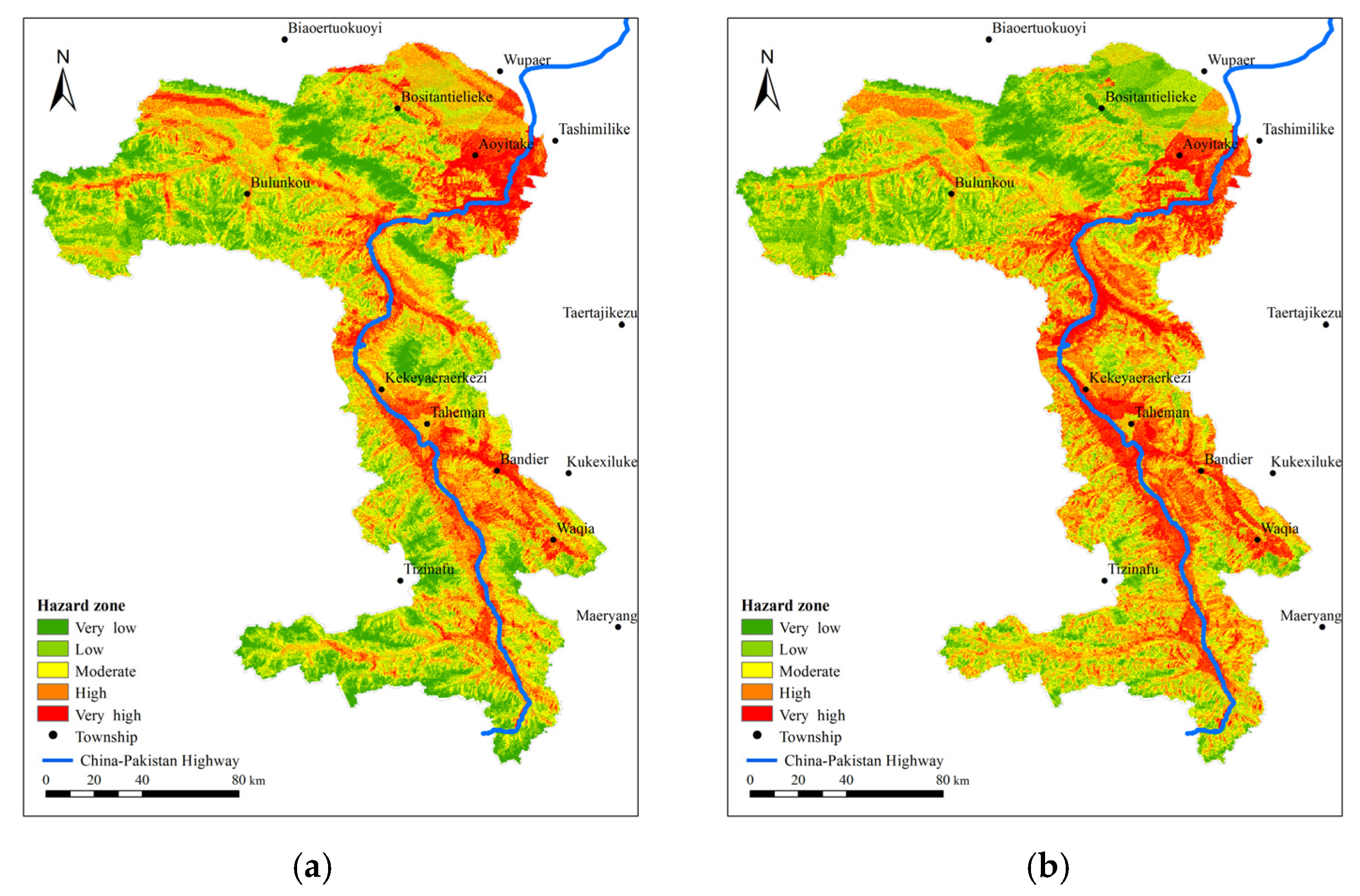
The natural breakpoint method was adopted to classify the hazard indexes into very high, high, medium, low, and very low hazard zones, according to the selected grading status of the debris flow disaster influence factors and the assessment model. The debris flow hazard grading maps of the frequency ratio model and the frequency ratio–logistic regression model were obtained, as shown in Figure 11.
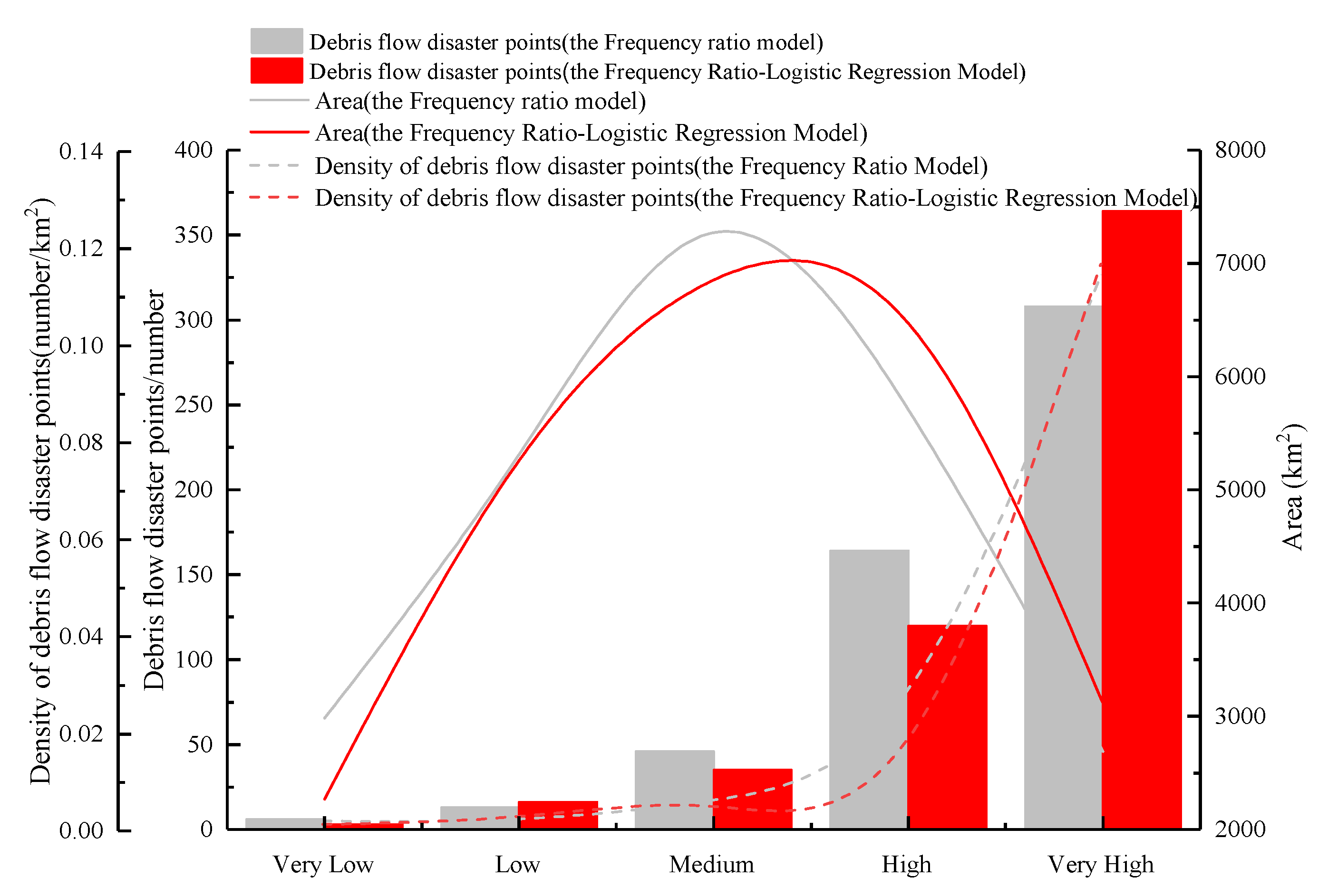
Figure 12 illustrates the variations in the distribution areas, debris flow disaster points, and disaster points density of different hazard zones for two models as the debris flow hazard level. It can be observed from the figure that the distribution areas of different hazard zones for two models initially increase and then decrease with the rise in hazard levels. Additionally, the number of debris flow disaster points and disaster points density for two models increase as the hazard level increases. However, the two models show differences in their calculation results. For the frequency ratio model, in the very high hazard zones, the distribution area, the proportion of debris flow disaster points, and the density of debris flow disaster points are 2688 km2 (11.2%), 57.4%, and 11.5 × 10⁻², respectively. In the high hazard zones, these values are 5706 km2 (23.8%), 30.5%, and 2.9 × 10⁻², respectively. In the medium hazard zone, these values are 7272 km2 (30.4%), 8.6%, and 0.6 × 10⁻², respectively. In the low hazard zones, these values are 5312 km2 (22.2%), 2.4%, and 0.2 × 10⁻², respectively. In the very low hazard zones, these values are 2982 km2 (12.4%), 1.1%, and 0.2 × 10⁻², respectively. For the frequency ratio–logistic regression coupled models, in the very high hazard zones, the distribution area, the proportion of debris flow disaster points, and the density of debris flow disaster points are 3114 km2 (13%), 67.7%, and 11.7 × 10⁻², respectively. In the high hazard zones, these values are 6469 km2 (27%), 22.3%, and 1.9 × 10⁻², respectively. In the medium hazard zones, these values are 6852 km2 (28.6%), 6.5%, and 0.5 × 10⁻², respectively. In the low hazard zones, these values are 5256 km2 (21.9%), 3%, and 0.3 × 10⁻², respectively. In the very low hazard zones, these values are 2269 km2 (9.5%), 0.6%, and 0.1 × 10⁻², respectively.
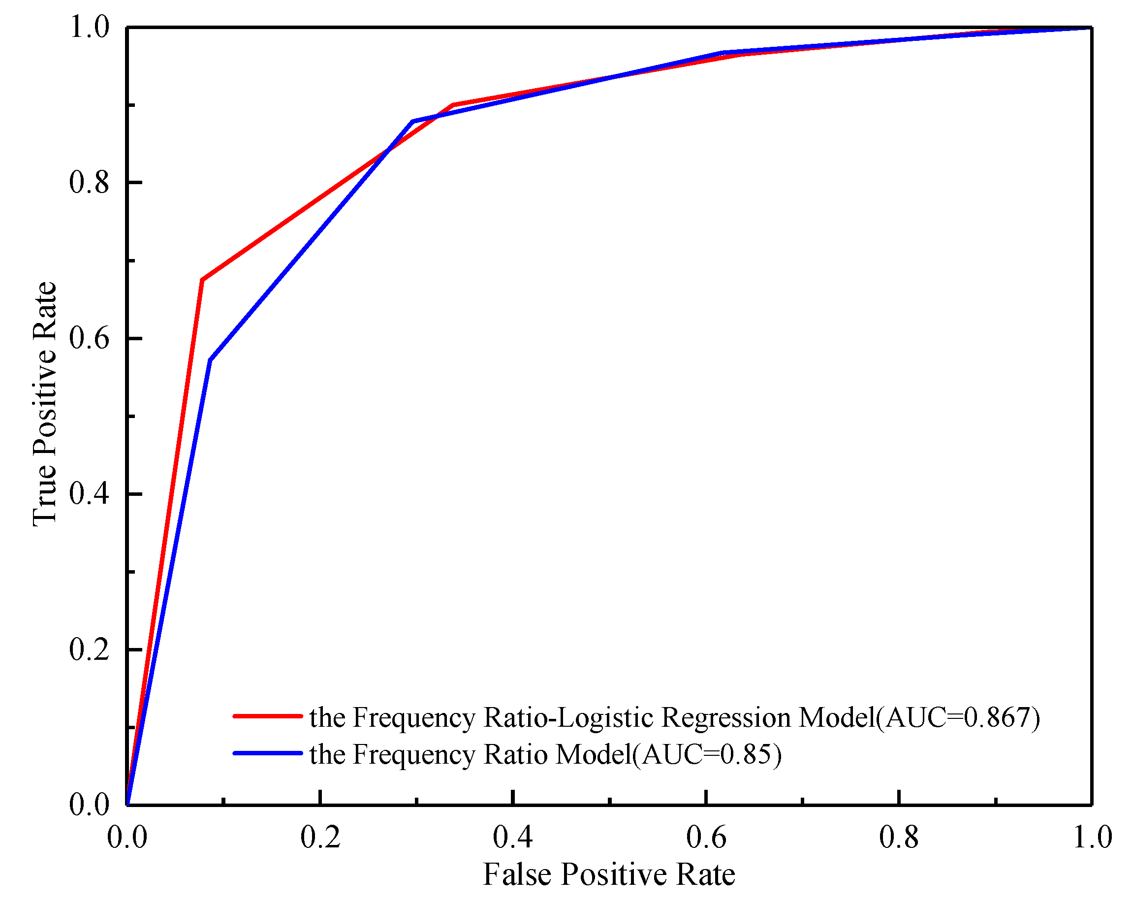
To evaluate the reliability of the model, Figure 13 presents the ROC curves of the frequency ratio model and the frequency ratio–logistic regression coupled model. The AUC values for the two models are 0.85 and 0.867, respectively, which shows that the accuracy of the coupled model is slightly higher than the single model. Therefore, the hazard results obtained from the frequency ratio–logistic regression coupled model is more accurate.
By analyzing the hazard assessment results of the frequency ratio–logistic regression coupled model, it was found that the debris flow hazard is largely distributed in a band along the Kashgar-to-Khunjerab section of the China–Pakistan Highway, with a small sporadic distribution in other areas. Very high hazard zones are mainly located in Aoyitake, Bulunkou, Kekeyaeraerkezi, and along the route. High hazard zones are scattered in Aoyitake, Bulunkou, Kekeyaeraerkezi, Taheman, and Tizinafu, while medium hazard zones are mainly located in Bositantielieke, Tashimilike, Bulunkou, Waqia, Bandier, Tizinafu, and Dabudaer. And low and very low hazard zones are located in Bulunkou, Bositantielieke, Yaoertuokuoyi, Tizinafu, Waqia, and other areas at the boundary.

4.2. Debris Flow Vulnerability Assessment

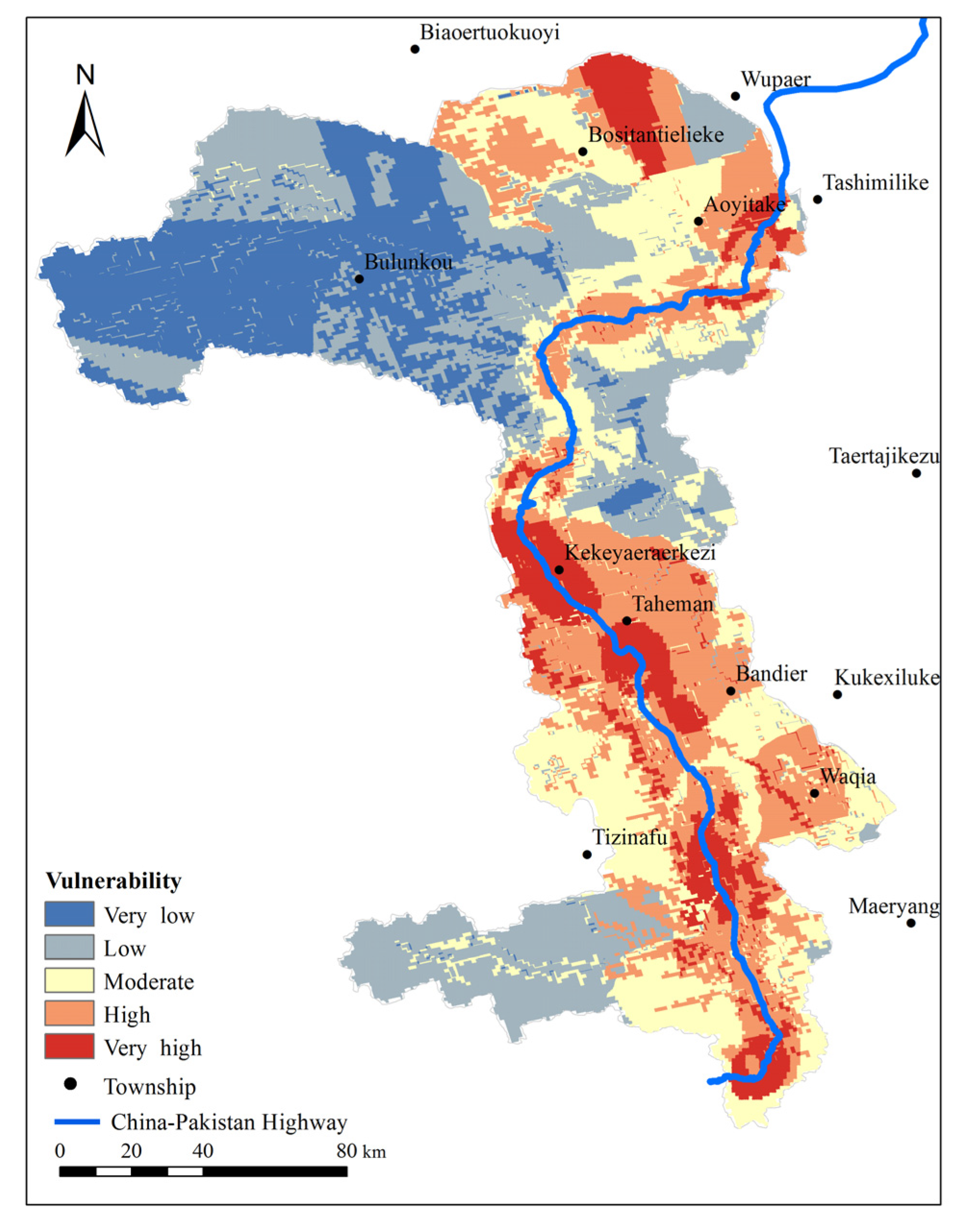
The vulnerability of the study area was obtained by integrating the exposure, sensitivity, and resilience. Based on the evaluation results of the vulnerability, the vulnerability was divided into five levels—very high, high, medium, low, and very low—by combining the distribution of debris flow disasters and the vulnerability characteristics of each township in the region, and the debris flow vulnerability grading map was obtained, as shown in Figure 14.
The vulnerability in the study area is generally concentrated in the township regions along the Kashgar-to-Khunjerab section of the China–Pakistan Highway. Very high vulnerability zones are mainly located in Kekeyaeraerkezi, Taheman, Tizinafu, and Dabudaer. High vulnerability zones involve eight townships, namely Aoyitake, Bulunkou, Kekeyaeraerkezi, Taheman, Dabudaer, Bandier, Waqia, and Yaoertuokuoyi. Medium vulnerability zones are mainly located in Yaoertuokuoyi, Bositantielieke, Aoyitake, Tizinafu, and Dabudaer. Low and very low vulnerability zones are mainly located in Bulunkou, Tizinafu, Wupaer, Aoyitake, and other areas in the north and southwest corner of the study area.
According to the vulnerability classification criteria, the area of very high vulnerability zones account for 9.7% of the total area; the high vulnerability zones account for 23.4%; the medium vulnerability zones account for 22.5%; the low vulnerability zones account for 26.3%; and the very low vulnerability zones account for 18.1%. The proportion of medium and above vulnerability zone areas reaches 55.6%, indicating relatively high vulnerability. The vulnerability assessment of the region provides further insights into the socioeconomic attributes of debris flows, offering valuable information for risk assessment of the Kashgar-to-Khunjerab section of the China–Pakistan Economic Corridor.

4.3. Debris Flow Risk Assessment

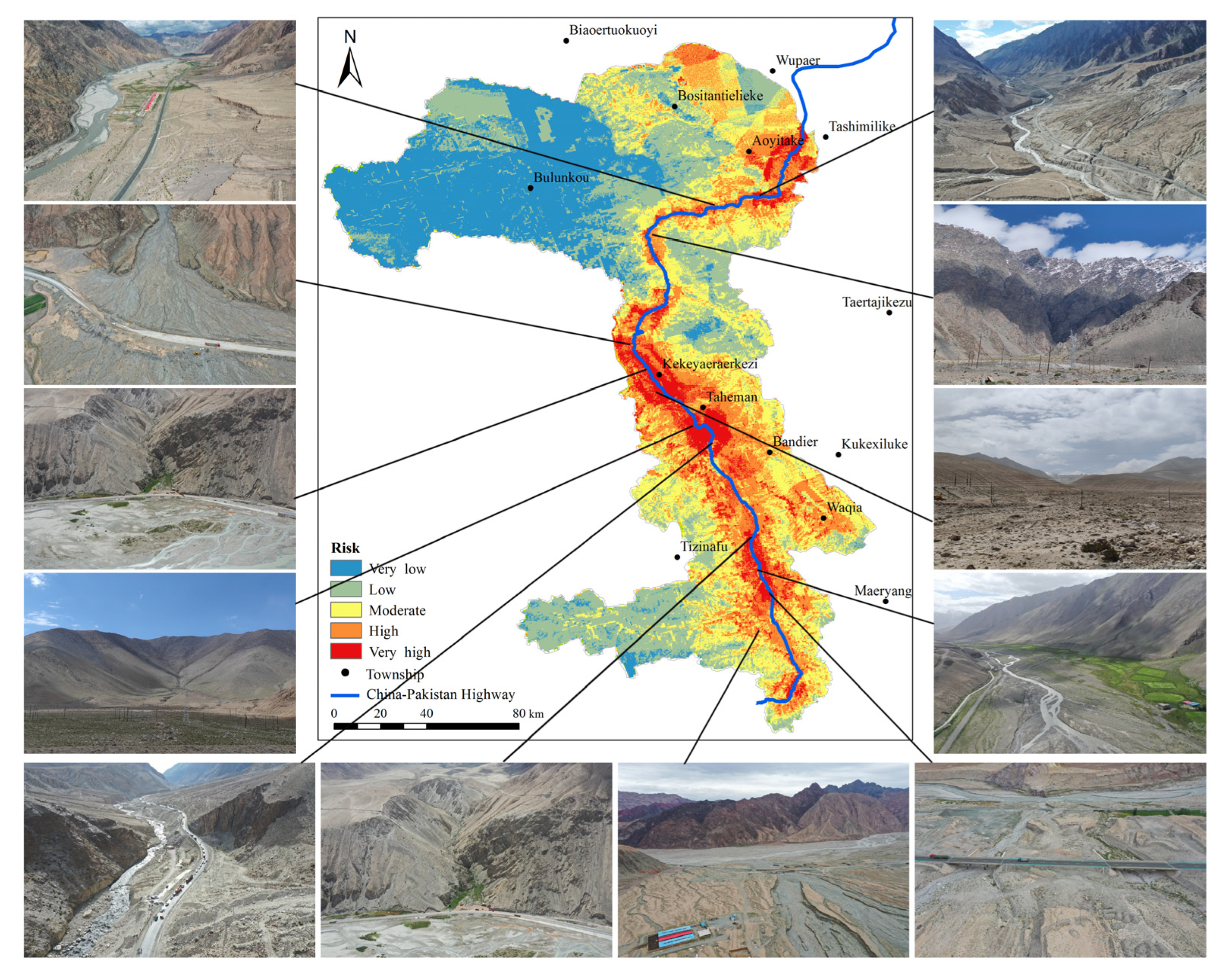
Figure 15 illustrates spatial distribution of debris flow risk in the study area. It can be observed that the risk levels generally radiate outward from the Kashgar-to-Khunjerab section of the China–Pakistan Highway, exhibiting a decreasing trend of from high to low. The very high risk zones are mainly distributed in a band across parts of in Aoyitake, Kekeyaeraerkezi, Taheman, and part of Tizinafu. The high risk zones have a similar distribution pattern to the very high risk zones and are mainly located in Bositantielieke, Waqia, Bandier, and other areas. The medium risk zones are mainly located in the towns and villages near the Kashgar-to-Khunjerab section of the China–Pakistan Highway, such as Aoyitake, Bulunkou, Bositantielieke, Kekeyaeraerkezi, Taheman, Tizinafu, Dabudaer, etc. The low and very low risk zones are mainly located in Bulunkou, Bositantielieke, and Tizinafu.
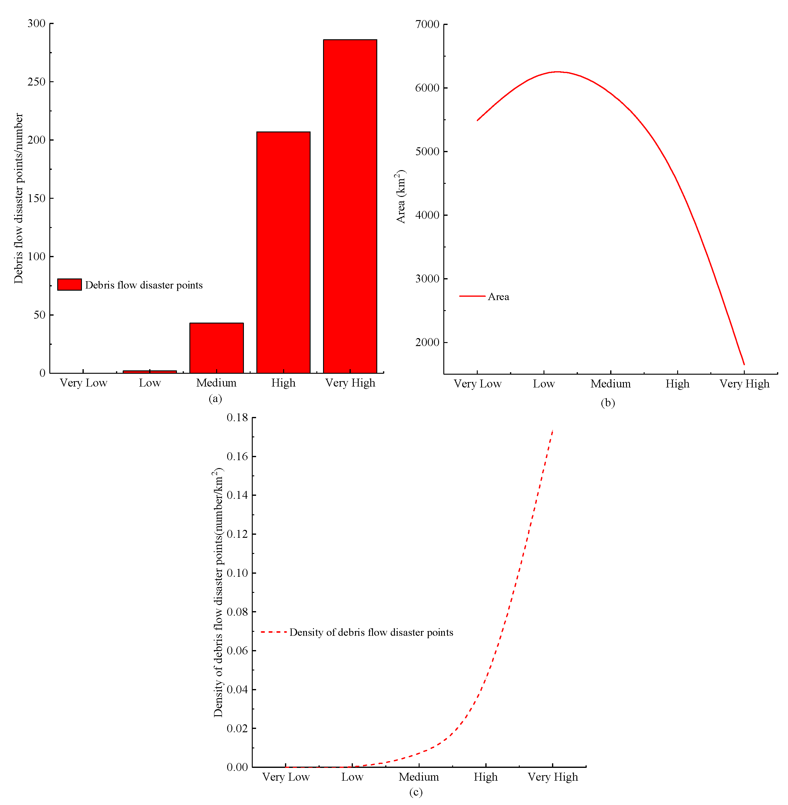
Figure 16 illustrates the variations in the distribution areas, debris flow disaster points, and disaster points density at different risk zones. It can be observed that the distribution areas of different risk zones initially increase and then decrease with the rise in risk levels. Additionally, the number of debris flow disaster points and disaster points density increase as the risk level increases. In the very high risk zone, the distribution area, the proportion of debris flow disaster points, the density of debris flow disaster points are 1661 km2 (6.9%), 53.2%, and 17.2 × 10⁻², respectively. In the high hazard zone, these values are 4548 km2 (19%), 38.5%, and 4.5 × 10⁻² respectively. In the medium hazard zone, these values are 5955 km2 (24.9%), 8%, and 0.7 × 10⁻², respectively. In the low hazard zone, these values are 6269 km2 (26.2%), 0.4%, and 0.03 × 10⁻², respectively. In the very low hazard zone, the distribution area is 5527 km2 (23.1%), and no debris flow disasters occurred. Based on the analysis of the aforementioned data, it is concluded that the area of medium risk zones and above accounts for 50.8% of the total area, and approximately 91.7% of debris flow disaster points are located in high and very high risk zones. This indicates that the overall risk level in the study area is high, with frequent occurrences of debris flow disasters. Through field investigations, it was found that one of the main reasons for the frequent debris flow events is the large accumulation of the solid loose materials from the debris flow channel [49], making it very easy for debris flow disasters to occur under short-term heavy rainfall conditions. On the other hand, the mountainous region in the northern part of the China–Pakistan Economic Corridor includes the Kush Mountains, the Himalayas, and the Karakorum Mountains, and three of the world’s seven major glaciers are located in this region [50]. However, most glaciers are rapidly thinning at a rate of 0.66 ± 0.09 m per year due to human activities and global warming [51]. The melting of glaciers and the increase in water volume also raise the probability of debris flow disasters. Therefore, the prevention and control of debris flow disasters should be strengthened in this study area.

5. Conclusions

This study analyzed field survey data and employed the frequency ratio and frequency ratio–logistic regression coupled model to evaluate the hazard of debris flows in the study area. The contribution weight model was used to evaluate the vulnerability of debris flows in the region. Based on the assessment results of hazard and vulnerability, a risk assessment model was utilized to explore the risk situation of debris flow disasters in the China–Pakistan Economic Corridor. The main conclusions are as follows:
(1)
The frequency ratio–logistic regression coupled model (AUC = 0.867) is more suitable than the frequency ratio model (AUC = 0.85) for debris flow disasters hazard assessment. the debris flow hazard is largely distributed in a band along the Kashgar-to-Khunjerab section of the China–Pakistan Highway, with a small sporadic distribution in other areas; the area of medium hazard zones and above accounts for 68.6% of the total area.
(2)
The vulnerability in the study area is generally concentrated in the township regions along the Kashgar-to-Khunjerab section of the China–Pakistan Highway. The proportion of medium and above vulnerability zones areas reaches 55.6%.
(3)
The risk levels of the study area generally radiate outward from the Kashgar-to-Khunjerab section of the China–Pakistan Highway, exhibiting a decreasing trend of from high to low. The distribution areas of different risk zones initially increase and then decrease with the rise in risk levels, and the number of debris flow disaster points and disaster points density increase as the risk level increases. The area of medium risk zones and above accounts for 50.8% of the total area. Approximately 91.7% of debris flow disaster points are located in high and very high risk zones. This indicates that the study area has a high level of risk, with frequent occurrences of debris flow disasters.

Author Contributions

Conceptualization, J.T. and Y.H.; methodology, X.S. and Y.H.; software, J.T. and Y.H.; validation, Z.Z. and X.L.; formal analysis, J.T. and Y.H.; investigation, X.S. and J.T.; data curation, F.L., X.Z. and X.L.; writing—original draft preparation, Y.H.; writing—review and editing, J.T. All authors have read and agreed to the published version of the manuscript.

Funding

This research was funded by Key Research and Development Project of Gansu Academy of Sciences grant number 2025GJHZ-02 and Youth Fund Gansu Academy of Sciences grant number 2024QN-02 and Natural Science Fund of Gansu Province Science and Technology Program grant number 24JRRA1139 and Research Startup Fund of Gansu Academy of Sciences grant number 2022QD-02. The APC was funded by Key Research and Development Project of Gansu Academy of Sciences.

Data Availability Statement

The original contributions presented in this study are included in the article. Further inquiries can be directed to the corresponding author.

Acknowledgments

The author would like to thank the data source institution, as well as the editor and reviewers for their valuable suggestions and constructive comments.

Conflicts of Interest

The authors declare no conflicts of interest.

Abbreviations

The following abbreviations are used in this manuscript:
ROCReceiver Operating Characteristic Curve
AUCArea Under the Curve

References

  1. Zou, Q.; Cui, P.; He, J.; Lei, Y.; Li, S. Regional risk assessment of debris flows in China-an HRU-based approach. Geomorphology 2019, 340, 84–102. [Google Scholar] [CrossRef]
  2. Jomelli, V.; Pavlova, I.; Giacona, F.; Zgheib, T.; Eckert, N. Respective influence of geomorphologic and climate conditions on debris-flow occurrence in the Northern French Alps. Landslides 2019, 16, 1871–1883. [Google Scholar] [CrossRef]
  3. Carrión-Mero, P.; Montalván-Burbano, N.; Morante-Carballo, F.; Quesada-Román, A.; Apolo-Masache, B. Worldwide Research Trends in Landslide Science. Int. J. Environ. Res. Public Health 2021, 18, 9445. [Google Scholar] [CrossRef] [PubMed]
  4. Jiang, Y.H.; Guo, Y.Q.; He, J.X. A dataset of distributions and characteristics of debris flows in the China-Pakistan Economic Corridor. Sci. Data Bank. 2021, 6, 1–10. [Google Scholar]
  5. Shu, H.P.; Qi, S.; Ning, N.; Ma, J.Z.; Zhang, P. Risk assessment of debris flow disaster: A case study of Wudu District in the south of Gansu Province, China. J. Nat. Disasters 2016, 25, 34–41. [Google Scholar]
  6. Liu, X.R.; Zhang, M.Y.; Zhou, Z.Q.; Su, X.; Ye, W.L.; Wen, T.; Zhang, G.X.; Liu, D. Nonlinear characteristics and disaster aggravation effects of debris flow evolution along the Chinese section of the China-Pakistan Highway. J. Lanzhou Univ. 2022, 58, 364–371. [Google Scholar]
  7. Zhou, Y.Y.; Yue, D.X.; Liang, G.; Li, S.Y.; Zhao, Y.; Chao, Z.Z.; Meng, X.X. Risk assessment of debris flow in a mountain-basin area, western China. Remote Sens. 2022, 14, 2942. [Google Scholar] [CrossRef]
  8. Varnes, D. Landslide Hazard Zonation: A Review of Principles and Practice. Nat. Hazards 1984, 3. [Google Scholar] [CrossRef]
  9. Shi, P.J. Theory and practice of disaster study. J. Nat. Disasters 1996, 5, 6–17. [Google Scholar]
  10. Lin, J.H.; Chen, W.H.; Qi, X.H.; Hou, H.R. Risk assessment and its influencing factors analysis of geological hazards in typical mountain environment. J. Clean. Prod. 2021, 309, 127077. [Google Scholar] [CrossRef]
  11. Huggel, C.; Kääb, A.; Haeberli, W.; Krummenacher, B. Regional-scale GIS- models for assessment of hazards from glacier lake outbursts: Evaluation and application in the Swiss Alps. Nat. Hazards Earth Syst. Sci. 2003, 3, 647–662. [Google Scholar] [CrossRef]
  12. Liu, X.L.; Lei, J.Z. A method for assessing regional debris flow risk: An application in Zhaotong of Yunnan province (SW China). Geomorphology 2003, 52, 181–191. [Google Scholar] [CrossRef]
  13. Chau, K.T.; Lo, K.H. Hazard assessment of debris flows for Leung King Estate of Hong Kong by incorporating GIS with numerical simulations. Nat. Hazards Earth Syst. Sci. 2004, 4, 103–116. [Google Scholar] [CrossRef]
  14. Bisson, M.; Favalli, M.; Fornaciai, A.; Mazzarini, F.; Isola, I.; Zanchetta, G.; Pareschi, M.T. A rapid method to assess fire-related debris flow hazard in the Mediterranean region: An example from Sicily (southern Italy). Int. J. Appl. Earth Obs. Geoinf. 2005, 7, 217–231. [Google Scholar] [CrossRef]
  15. Shi, P.J.; Zou, M.; Li, B.J.; Zhou, J.H.; Wang, Y. Regional safety construction and risk management system: The actuality and trend of the study of disaster and risk based on the world congress on risk. Adv. Earth Sci. 2005, 20, 173–179. [Google Scholar]
  16. Blahut, J.; Glade, T.; Sterlacchini, S. Debris flows risk analysis and direct loss estimation: The case study of Valtellina di Tirano, Italy. J. Mt. Sci. 2014, 11, 288–307. [Google Scholar] [CrossRef]
  17. Tang, C.; Zhang, J.; Wan, S.Y.; Zhou, C.H. Loss Evaluation of Urban Debris Flow Hazard Using High Spatial Resolution Satellite Imagery. Sci. Geogr. Sin. 2006, 26, 358–363. [Google Scholar]
  18. Lin, J.-Y.; Yang, M.-D.; Lin, B.-R.; Lin, P.-S. Risk assessment of debris flows in Songhe Stream, Taiwan. Eng. Geol. 2011, 123, 100–112. [Google Scholar] [CrossRef]
  19. Liang, W.-J.; Zhuang, D.-F.; Jiang, D.; Pan, J.-J.; Ren, H.-Y. Assessment of debris flow hazards using a bayesian network. Geomorphology 2012, 171, 94–100. [Google Scholar] [CrossRef]
  20. Zhao, Y.; Meng, X.; Qi, T.; Chen, G.; Li, Y.; Yue, D.; Qing, F. Modeling the Spatial Distribution of Debris Flows and Analysis of the Controlling Factors: A Machine Learning Approach. Remote Sens. 2021, 13, 4813. [Google Scholar] [CrossRef]
  21. Asghar, M.; Pasha, G.A.; Ghani, U.; Iqbal, S.; Jameel, M.S. Investigating multiple debris impact load and role of vegetation in protection of house model during floods. In Proceedings of the 2nd Conference on Sustainability in Civil Engineering, Islamabad, Pakistan, 12 August 2020; Volume 7. [Google Scholar]
  22. Liu, F.Z.; Cui, C.; Wang, J.C.; Cao, Y.F.; Li, W. Hazard assessment of debris flow based on the certainty factor rate and the logistic regression model. J. Saf. Environ. 2021, 21, 1693–1703. [Google Scholar]
  23. Ouyang, C.J.; Wang, Z.W.; An, H.C.; Liu, X.R.; Wang, D.P. An example of a hazard and risk assessment for debris flows—A case study of Niwan Gully, Wudu, China. Eng. Geol. 2019, 263, 105351. [Google Scholar] [CrossRef]
  24. Chu, H.B.; Mu, H.D.; Wang, J.Z. Application of analytic hierarchy process on zoning hazard degree of geologic disaster in Taihang Mountain region. Chin. J. Geol. Hazard Control 2003, 14, 125–129. [Google Scholar]
  25. Liu, Y.; Tang, C.; Feng, Y. Geological Disaster Risk Assessment Based on AHP Information Method. Earth Environ. 2013, 41, 173–179. [Google Scholar]
  26. Jena, R.; Pradhan, B.; Beydoun, G.; Nizamuddin; Ardiansyah; Sofyan, H.; Affan, M. Integrated model for earthquake risk assessment using neural network and analytic hierarchy process: Aceh Province, Indonesia. Geosci. Front. 2020, 11, 613–634. [Google Scholar] [CrossRef]
  27. Wang, Z.F.; Zhang, T.S.; Wang, L.; Tang, Z.Y. The integrated assessment system of ecogeological environmental carrying capacity for Dujiangyan-Wenchuan Highway. Surv. Mapp. 2016, 41, 77–81. [Google Scholar]
  28. Sujatha, E.R.; Sridhar, V. Mapping debris flow susceptibility using analytical network process in Kodaikkanal Hills, Tamil Nadu (India). J. Earth Syst. Sci. 2017, 126, 116. [Google Scholar] [CrossRef]
  29. Xu, W.B.; Yu, W.J.; Jing, S.C.; Zhang, G.P.; Huang, J.X. Debris flow susceptibility assessment by GIS and information value model in a large-scale region, Sichuan Province (China). Nat. Hazards 2013, 65, 1379–1392. [Google Scholar] [CrossRef]
  30. Wu, C.R.; Jiao, Y.M.; Wang, J.L.; Xu, H.H.; Zhang, H.; Xu, Q.E. Frequency ratio and logistic regression models based coupling analysis for susceptibility of landslide in Shuangbai County. J. Nat. Disasters 2021, 30, 213–224. [Google Scholar]
  31. Gu, C.J.; Sun, S.; Ning, N.; Ma, J.Z. Research on Debris Flow Disaster Vulnerability Based on the Production. Mt. Res. Dev. 2015, 33, 303–310. [Google Scholar]
  32. Gu, C.J.; Sun, S.; Ma, J.Z. Debris flow vulnerability assessment based on DEA model and production function. J. Lanzhou Univ. 2014, 50, 751–756. [Google Scholar]
  33. Li, L.F.; Wang, J.F.; Leung, H.; Zhao, S.S. A Bayesian Method to Mine Spatial Data Sets to Evaluate the Vulnerability of Human Beings to Catastrophic Risk. Risk Anal. 2012, 32, 1072–1092. [Google Scholar] [CrossRef] [PubMed]
  34. Chen, P.; Chen, X.L. Summary on Research of Coupled Human-Environment System Vulnerability under Global Environmental Change. Prog. Geogr. 2010, 29, 454–462. [Google Scholar]
  35. Ding, M.T.; Heiser, M.; Hübl, J.; Fuchs, S. Regional vulnerability assessment for debris flows in China-a CWS approach. Landslides 2016, 13, 537–550. [Google Scholar] [CrossRef]
  36. Cui, P.; Xang, L.-Z.; Zou, Q. Risk assessment of highways affected by debris flows in Wenchuan earthquake area. J. Mt. Sci. 2013, 10, 173–189. [Google Scholar] [CrossRef]
  37. Gao, Z.M.; Ding, M.T.; Huang, T.; Hu, X.W. Geohazard vulnerability assessment in Qiaojia seismic zones, SW China. Int. J. Disaster Risk Reduct. 2021, 52, 101928. [Google Scholar] [CrossRef]
  38. Zhu, Y.Y.; Yang, Z.Q.; Liao, L.P.; Steve, Z.; Muhammad, W.; Ye, C.Y.; Chen, H.P.; Pang, M. Glacialized geomorphologcial geohazard along China-Pakistan International Karakoram Highway. J. Catastrophol. 2014, 29, 81–90. [Google Scholar]
  39. Wei, X.L.; Chen, B.C.; Chen, R.K.; Li, B.; Yang, X.L.; Yang, L.H. Rainfall pattern and critical threshold of rainfall type debris flow in Gezi river section of China Pakistan Highway. J. Catastrophol. 2018, 33, 75–80. [Google Scholar]
  40. Wei, X.L.; Chen, B.C.; Li, B.; Luo, W.G. Hazard assessment and prevention analysis of debris flows along Aoyitage-Blulunkou section of Sino-Pakisstan highway. Highway 2018, 11, 14–20. [Google Scholar]
  41. Han, R.; Feng, C.-C.; Xu, N.; Guo, L. Spatial heterogeneous relationship between ecosystem services and human disturbances: A case study in Chuandong, China. Sci. Total Environ. 2020, 721, 137818. [Google Scholar] [CrossRef]
  42. Gao, J.P.; Shi, X.Y.; Li, L.H.; Zhou, Z.Q.; Wang, J.F. Assessment of landslide susceptibility using different machine learning methods in Longnan City, China. Sustainability 2022, 14, 16716. [Google Scholar] [CrossRef]
  43. Chang, M.; Tang, C.; Van Asch, T.W.; Cai, F. Hazard assessment of debris flows in the Wenchuan earthquake-stricken area, South West China. Landslides 2017, 14, 1783–1792. [Google Scholar] [CrossRef]
  44. Zhang, Y.H.; Ge, T.T.; Tian, W.; Liou, Y.A. Debris Flow Susceptibility Mapping Using Machine-Learning Techniques in Shigatse Area, China. Remote Sens. 2019, 11, 2801. [Google Scholar] [CrossRef]
  45. Du, S.X.; Wu, R.Y.; Sun, H.W.; Yan, D.; Xue, J.; Liao, W.H.; Chen, H.R. Analysis of extreme precipitation events along the China-Pakistan Economic Corridor. Trans. Chin. Soc. Agric. Eng. 2022, 38, 152–160. [Google Scholar]
  46. Li, Z.T.; Wang, T.; Zhou, Y.; Liu, J.M.; Xin, P. Landslide Susceptibility Assessment Based on Information Value Model, Logistic Regression Model and Their Integrated Model: A Case in Shatang River Basin, Qinghai Province. Geoscience 2019, 33, 235–245. [Google Scholar]
  47. Liu, X.L.; Miao, C.; Tian, C.S.; Qiu, J.A. Comparative Analysis of Risk Assessment of Landslides and Debris Flows of China in 2000 and 2010. Adv. Earth Sci. 2016, 31, 926–936. [Google Scholar]
  48. Liu, X.L.; Chen, Y.J. Application of Debris Flow Risk Zonation: An Example of West Sichuan. Sci. Geogr. Sin. 2010, 30, 558–565. [Google Scholar]
  49. Zou, Q.; Guo, X.J.; Luo, Y.; Jiang, Y.J.; Cui, P.; Su, L.J.; OU, G.Q.; Pan, H.L.; Liu, W.M. Spatial Pattern and Response of Landslide and Debris Flow Risks in China-Pakistan Economic Corridor. Bull. Chin. Acad. Sci. 2021, 36, 160–169. [Google Scholar]
  50. Baig, S.U.; Khan, H.; Din, A. Spatio-temporal Analysis of Glacial Ice Area Distribution of Hunza River Basin, Karakoram region of Pakistan. Hydrol. Process. 2018, 32, 1491–1501. [Google Scholar] [CrossRef]
  51. Kaab, A.; Berthier, E.; Nuth, C.; Gardelle, J.; Arnaud, Y. Contrasting Patterns of Early Twenty-first-century Glacier Mass Change in the Himalayas. Nature 2012, 488, 495–498. [Google Scholar] [CrossRef]
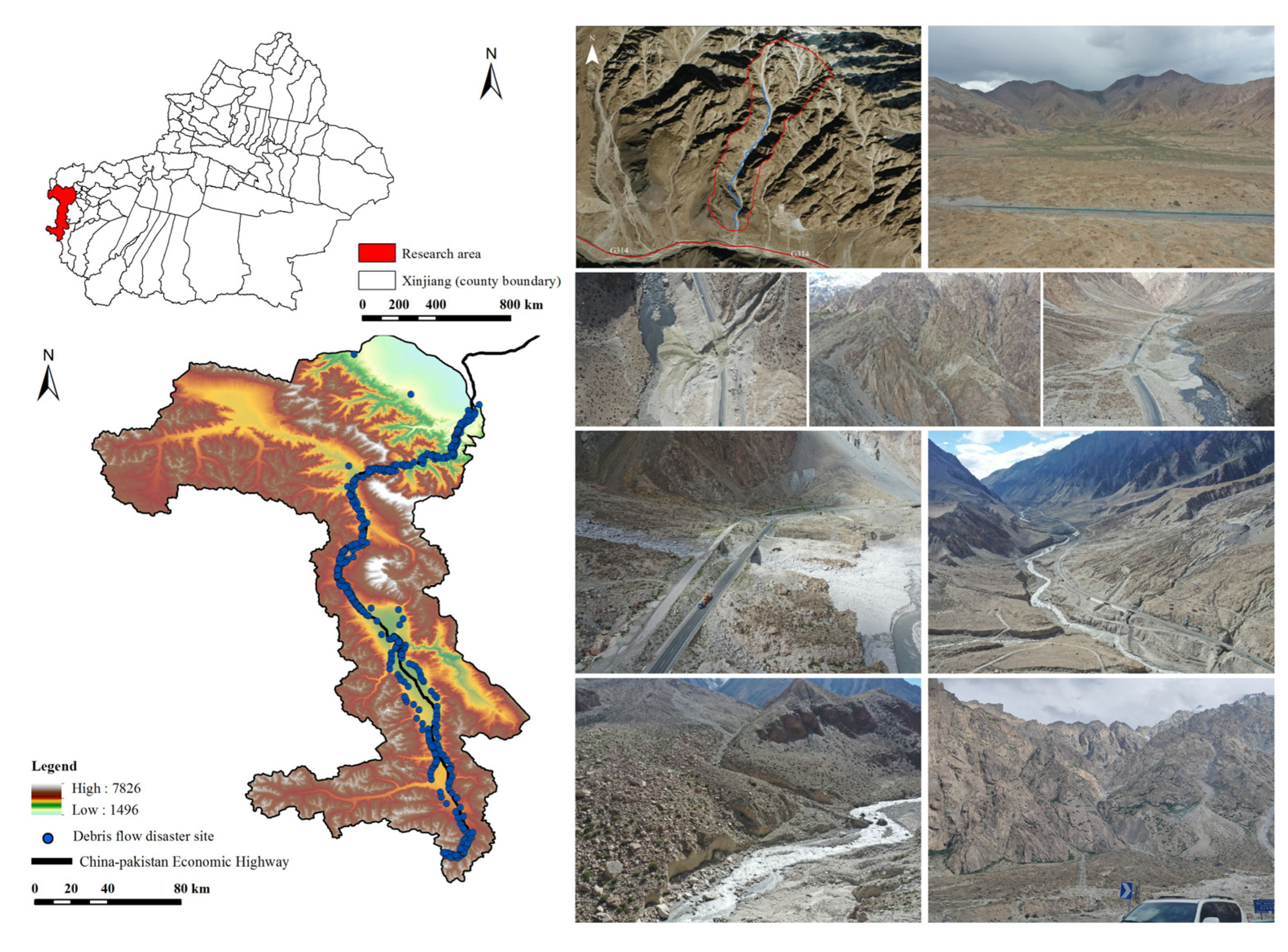
Figure 1. Distribution of debris flow disasters in the study area.
Water 17 02841 g001
Figure 2. Flow chart of this study.
Water 17 02841 g002
Figure 3. Distribution of four topographic factors. (a) elevation, (b) elevation difference, (c) aspect, (d) slope.
Water 17 02841 g003
Figure 4. Distribution of geological factors. (a): lithology, (b) distance to faults.
Water 17 02841 g004
Figure 5. Distribution of vegetation and soil factors. (a) NDVI, (b) soil type.
Water 17 02841 g005
Figure 6. Distribution of climatic conditions factors. (a) annual mean precipitation, (b) annual mean temperature.
Water 17 02841 g006
Figure 7. Distribution of human activities and others. (a) land use type, (b) distance to rivers.
Water 17 02841 g007
Figure 8. Distribution of exposure. (a) relative spatial location of debris flow, (b) density of debris flow hazard points.
Water 17 02841 g008
Figure 9. Distribution of the sensitivity. (a) density of road network, (b) density of population.
Water 17 02841 g009
Figure 10. Distribution of resilience. (a) GDP, (b) distance to town.
Water 17 02841 g010
Figure 11. Debris flow hazard maps based on two models. (a) the frequency ratio model; (b) the frequency ratio–logistic regression model.
Water 17 02841 g011
Figure 12. Comparison of the number of debris flow and density between the two models.
Water 17 02841 g012
Figure 13. ROC curves based on two models.
Water 17 02841 g013
Figure 14. Debris flow vulnerability maps based on the contributing weight superposition model.
Water 17 02841 g014
Figure 15. Spatial distribution of debris flow risk.
Water 17 02841 g015
Figure 16. The variations in debris flow disaster points, areas and density of debris flow disaster points at different risk zones. (a) debris flow disaster points; (b) area; (c) density of debris flow disaster points.
Water 17 02841 g016
Table 1. Data sources for debris flow disasters hazard assessment indicators.
CategoryIndicatorsUnitScale/ResolutionSource
TopographyElevationm30 mGeospatial Data Cloud
30 May 2024
(http://www.gscloud.cn/search)
elevation differencem
Slope°
Aspect/
Geological structureLithology/1:250,000National Geological Data Museum
30 May 2024
(https://www.ngac.cn/125cms/c/qggnew/index.htm)
Distance to faultsm1:250,000
Surface vegetation and soilNDVI/1:250,000Modis/terra Data
30 May 2024
(https://ladsweb.nascom.nasa.gov/search)
Soil type/1:1,000,000National Cryosphere Desert Data Center
30 May 2024
(http://www.ncdc.ac.cn)
Climatic conditionsAnnual mean precipitationmm1000 mResource and Environmental Science Data Platform
30 May 2024
(https://www.resdc.cn/)
Annual mean temperature°C1000 m
Human activities and othersLand use/30 mNational Catalogue Service For Geographic Information
30 May 2024
(https://www.webmap.cn/commres.do?method=globeDetails&type=EasyAccess)
Distance to riversm1:250,000National Catalogue Service For Geographic Information
30 May 2024
(https://www.webmap.cn/main.do?method=index)
Table 2. Data sources for debris flow disasters vulnerability assessment indicators.
CategoryIndicatorsUnitScale/ResolutionSource
Exposurerelative spatial position of debris flowm30 mInstitute of Geological Natural Disaster Prevention and Control, Gansu Academy of Sciences
density of debris flow disaster pointsm30 m
Sensitivitydensity of road network/30 mNational Catalogue Service For Geographic Information
30 May 2024
(https://www.webmap.cn/main.do?method=index)
density of populationPeople/km21000 m
ResilienceGDP10,000 CNY/km21000 mNational Catalogue Service For Geographic Information
30 May 2024
(https://www.webmap.cn/main.do?method=index)
distance to townm30 m
Disclaimer/Publisher’s Note: The statements, opinions and data contained in all publications are solely those of the individual author(s) and contributor(s) and not of MDPI and/or the editor(s). MDPI and/or the editor(s) disclaim responsibility for any injury to people or property resulting from any ideas, methods, instructions or products referred to in the content.