Article

Daily Runoff Prediction Method Based on Secondary Decomposition and the GTO-Informer-GRU Model

1
Electric Power Research Institute, Yunnan Power Grid Co., Ltd., China Southern Power Grid, Kunming 650220, China
2
Department of Mechanical Engineering, Baoding Campus, North China Electric Power University, Baoding 071066, China
*
Author to whom correspondence should be addressed.
Water 2025, 17(18), 2775; https://doi.org/10.3390/w17182775
Submission received: 28 August 2025 / Revised: 16 September 2025 / Accepted: 18 September 2025 / Published: 19 September 2025

Abstract

Hydrological runoff prediction serves as the core technological foundation for water resource management and flood/drought mitigation. However, the nonlinear, non-stationary, and multi-temporal scale characteristics of runoff data result in insufficient accuracy of traditional prediction methods. To address the challenges of single decomposition methods’ inability to effectively separate multi-scale components and single deep learning models’ limitations in capturing long-range dependencies or extracting local features, this study proposes an Informer-GRU runoff prediction model based on STL-CEEMDAN secondary decomposition and Gorilla Troops Optimizer (GTO). The model extracts trend, seasonal, and residual components through STL decomposition, then performs fine decomposition of the residual components using CEEMDAN to achieve effective separation of multi-scale features. By combining Informer’s ProbSparse attention mechanism with GRU’s temporal memory capability, the model captures both global dependencies and local features. GTO is introduced to optimize model architecture and training hyperparameters, while a multi-objective loss function is designed to ensure the physical reasonableness of predictions. Using daily runoff data from the Liyuan Basin in Yunnan Province (2015–2023) as a case study, the results show that the model achieves a coefficient of determination (R2) and Nash-Sutcliffe efficiency coefficient (NSE) of 0.9469 on the test set, with a Kling-Gupta efficiency coefficient (KGE) of 0.9582, significantly outperforming comparison models such as LSTM, GRU, and Transformer. Ablation experiments demonstrate that components such as STL-CEEMDAN secondary decomposition and GTO optimization enhance model performance by 31.72% compared to the baseline. SHAP analysis reveals that seasonal components and local precipitation station data are the core driving factors for prediction. This study demonstrates exceptional performance in practical applications within the Liyuan Basin, providing valuable insights for water resource management and prediction research in this region.

1. Introduction

Hydrological runoff forecasting plays a pivotal role in water resource management, flood and drought mitigation, and hydraulic infrastructure planning. Accurate runoff prediction is essential for optimizing reservoir operations, agricultural irrigation scheduling, ensuring water supply security, and issuing timely flood warnings. It serves as a scientific foundation for the sustainable utilization of water resources [1,2,3,4,5]. However, under the intensifying impacts of climate change and the increasing frequency of extreme weather events, runoff dynamics—shaped by precipitation, evaporation, soil properties, vegetation cover, and anthropogenic activities—exhibit pronounced nonlinearity, nonstationarity, and spatiotemporal variability. These complexities challenge the predictive accuracy of traditional hydrological models. Faced with the dual pressure of uncertainty and hydrological prediction challenges [6,7], it has become a core topic in the field of hydrological prediction to develop more adaptive runoff prediction models to achieve accurate prediction.
Deep learning can effectively identify the mapping relationship between input and output variables, and has strong nonlinear fitting ability. It is widely used in the field of runoff prediction [8,9,10]. For instance, Wilbrand et al. [11] trained Long Short-Term Memory (LSTM) models on global datasets such as ERA5 and CAMELS-US to forecast runoff in ungauged basins, showcasing the model’s generalization and scalability. Clark et al. [12] benchmarked LSTM against conceptual hydrological models across 500 Australian basins, revealing superior performance in generalization and drought-period prediction. Wang et al. [13] employed a feedback-enhanced Gated Recurrent Unit (GRU) variant to improve flood forecasting in fast-response basins. Xu et al. [14] integrated wavelet transforms with Transformer architectures to achieve high-precision monthly runoff predictions, particularly excelling in peak flow estimation. Jia et al. [15] combined GRU with robust local mean decomposition and slime mold optimization to enhance monthly runoff forecasting in the Yiluo River Basin, China. Wang et al. [16] incorporated baseflow separation techniques into Transformer models, improving long-lead runoff prediction in the Yellow River Basin.
Despite these advances, due to the nonlinearity and nonstationarity of runoff data, the original data is still insufficient for prediction in deep learning model. To address this, Zhang et al. [17] integrated decomposition techniques such as Variational Mode Decomposition (VMD), Empirical Mode Decomposition (EMD) and Wavelet Analysis (WA) with long LSTM networks, identifying VMD-LSTM as the most effective combination over 41 years of data. Xu et al. [14] decomposed runoff into intrinsic mode functions (IMFs) using VMD, then applied CNN and BiLSTM with Bayesian optimization to significantly improve prediction accuracy. He et al. [18] proposed the SD-GRU model, which decomposes runoff into seasonal components prior to GRU modeling, yielding enhanced precision and robustness. Wang et al. [19] utilized STL to preprocess inflow data into trend and seasonal components, improving LightGBM’s predictive performance for Bohai Bay inflows. Aerts et al. [20] applied CEEMDAN decomposition to enhance GRU-based flood forecasting in mountainous regions.
While combining single decomposition methods with deep learning architectures has improved predictive accuracy, notable limitations persist. Regarding decomposition: runoff data encompasses interannual, seasonal, monthly, and weekly variability, with overlapping periodic components across scales. Single decomposition techniques struggle to isolate and identify these multi-scale patterns effectively. Moreover, the runoff process contains linear trend and complex nonlinear change, which can not be adequately processed by traditional linear decomposition methods. For example, STL can not adequately deal with the nonlinear high-frequency components in the residual, while the residual often contains important high-frequency information and abnormal event information. Ignoring the residual leads to information loss [21]. Regarding deep learning models: although LSTM can model long-term dependencies, it suffers from high computational complexity, low training efficiency, and susceptibility to overfitting due to its large parameter space, with gradient propagation issues in long sequences. GRU lacks global modeling capacity and struggles to capture long-range dependencies. Transformer models, despite their powerful attention mechanisms, are limited in extracting localized temporal features [22]. Furthermore, model performance is highly sensitive to architectural design and hyperparameter configuration. Traditional manual tuning and grid search methods are inefficient in high-dimensional parameter spaces and prone to local optima, constraining further performance gains [23].
To address these challenges, this study proposes an Informer-GRU runoff prediction model based on STL-CEEMDAN secondary decomposition and artificial gorilla force optimizer (GTO). At the time series decomposition level, this paper combines the advantages of STL and CEEMDAN to dig and extract information from complex hydrological time series layer by layer. At the deep learning architecture level, residual connections and layer normalization are introduced to integrate Informer’s ProbSparse attention mechanism with deep GRU networks, forming a hybrid architecture capable of capturing both long-range dependencies and localized temporal features. For model optimization, the Gorilla Troops Optimizer (GTO) is employed to perform intelligent global parameter search, automatically tuning architectural parameters (e.g., number of hidden layers, neurons, attention heads) and training hyperparameters (e.g., learning rate, batch size, loss weights). A multi-objective loss function incorporating hydrology-specific metrics is designed to ensure the physical plausibility of predictions. The primary objectives of this research are to:
(1)
Develop a high-precision daily runoff prediction methodology specifically tailored for water resource management in the Liyuan Basin, Yunnan Province;
(2)
Investigate the effectiveness of STL-CEEMDAN secondary decomposition in processing complex hydrological time series with multi-scale variability;
(3)
Validate the superiority of the GTO-optimized Informer-GRU hybrid architecture in capturing both global and local temporal patterns in runoff dynamics;
(4)
Provide a comprehensive technical framework and practical insights for water resource management and flood control in similar plateau mountainous watersheds.
The proposed methodology demonstrates exceptional performance in the Liyuan Basin case study, achieving coefficient of determination (R2) and Nash-Sutcliffe efficiency (NSE) values of 0.947 with Kling-Gupta efficiency (KGE) of 0.958. These findings contribute practical insights and technical guidance for water resource management strategies, reservoir operation optimization protocols, and flood risk assessment frameworks applicable to extensive regions throughout Yunnan Province and hydrologically similar mountainous watersheds with comparable climatic conditions.

2. Study Area and Data Sources

The Liyuan Basin in Yunnan Province is selected as the case study area (Figure 1). The Liyuan Basin is located in northwestern Yunnan Province, situated in the transition zone between the southeastern edge of the Qinghai-Tibet Plateau and the Yunnan-Guizhou Plateau, belonging to a typical plateau mountain subtropical monsoon climate zone. The input data for this study consists of precipitation and runoff data. Runoff data uses measured daily runoff data from the inflow control section at the Liyuan Hydropower Station outlet, with units in cubic meters per second (m3/s). Precipitation data comes from measured daily precipitation data from 6 rain gauge stations within the Liyuan Basin (TuGong, XiaoZhongDian, XiaRuo, BaiDi, BenZiLan, GeZan), spanning from 1 January 2015, to 31 December 2023, totaling 3287 days.
It should be noted that the rain gauges are primarily concentrated in the lower portion of the watershed, which reflects practical constraints of gauge installation and maintenance in mountainous terrain. However, this spatial limitation is addressed through several aspects of our methodology: (1) The STL-CEEMDAN decomposition extracts robust seasonal and trend patterns that are less sensitive to spatial sampling density; (2) The six gauges capture the main precipitation gradient from upstream to downstream within the basin; (3) The hierarchical decomposition approach focuses on temporal pattern extraction rather than spatial interpolation, making it more resilient to spatial bias in gauge distribution. While future research could benefit from additional upstream gauges, our results demonstrate that the current network provides sufficient information for accurate runoff prediction in this basin.

3. Research Methods

3.1. Time Series Secondary Decomposition

Time series decomposition is an important means to extract the potential information of time series data. By decomposing the complex original sequence into trend, seasonality, periodicity and residual components, we can better understand the internal laws of the data. In hydrological prediction, runoff time series typically contain variation patterns at multiple temporal scales: long-term trends reflect the influence of basin underlying surface conditions and climate change, seasonal variations embody the annual distribution characteristics of precipitation and temperature, and short-term fluctuations correspond to specific rainfall-runoff events [24]. Based on runoff data characteristics and the limitations of single decomposition, this study adopts a secondary decomposition framework combining STL and CEEMDAN.

3.1.1. STL Decomposition Method

STL decomposition (Seasonal and Trend decomposition using Loess) iteratively separates trend (T), seasonality (S), and residual (R) through locally weighted regression [25]. The calculation formula is as follows:
X ( t ) = T ( t ) + S ( t ) + R ( t )
where X ( t ) is the original time series, T ( t ) is the trend component, S ( t ) is the seasonal component, and R ( t ) is the residual component.
STL decomposition uses an iterative algorithm that achieves decomposition by alternately fitting seasonal and trend components:
Step 1 Seasonal component extraction:
S ( k ) ( t ) = L o e s s s e a s o n a l ( X ( t ) T ( k 1 ) ( t ) )
Step 2 Trend component extraction:
T ( k ) ( t ) = L o e s s t r e n d ( X ( t ) S ( k ) ( t ) )
Step 3 Residual calculation:
R ( k ) ( t ) = X ( t ) T ( k ) ( t ) S ( k ) ( t )
where L o e s s s e a s o n a l and L o e s s t r e n d represent locally weighted regression for seasonal and trend fitting respectively, and k represents the iteration number.

3.1.2. CEEMDAN Decomposition Method

CEEMDAN (Complete Ensemble Empirical Mode Decomposition with Adaptive Noise) is an improved version of EMD that effectively solves mode mixing problems by adding adaptive white noise [26]. The calculation process is as follows:
Given input signal R ( t ) (residual from STL decomposition), CEEMDAN decomposition decomposes it into n Intrinsic Mode Functions (IMFs) and one residual term:
R ( t ) = i = 1 n I M F i ( t ) + r n ( t )
First-order IMF extraction:
I M F 1 ( t ) = 1 I i = 1 I E 1 ( R ( t ) + β 0 E 1 ( w ( i ) ( t ) ) )
k-th order IMF extraction (k ≥ 2):
I M F k ( t ) = 1 I i = 1 I E 1 ( R e s k 1 ( t ) + β k 1 E k ( w ( i ) ( t ) ) )
where: E k ( ) represents the k-th mode operator of EMD decomposition, w ( i ) ( t ) represents the i-th white noise sequence, β k represents the k-th noise standard deviation coefficient, I represents the ensemble averaging times, and R e s k 1 ( t ) represents the residual signal from the (k − 1)-th step.
Residual signal update:
R e s k ( t ) = R e s k 1 ( t ) I M F k ( t )
IMF selection strategy: To avoid redundant information and noise interference, this study designs a selection method for important IMF components based on energy contribution. The energy contribution of each IMF is calculated, and the top several components with high energy proportions are selected as input features [27].
Energy calculation: E n e r g y k = t 1 T I M F k 2 ( t )
Importance proportion: I m p o r t a n c e k = E n e r g y k j = 1 k E n e r g y j

3.1.3. STL-CEEMDAN Joint Decomposition

The STL-CEEMDAN joint decomposition framework adopted in this study can be expressed as:
X ( t ) = T ( t ) + S ( t ) + i = 1 n I M F i ( t ) + r n ( t )
The first step uses STL decomposition to extract clear trend and seasonal components from the runoff sequence, which have good interpretability and stability. The second step applies CEEMDAN decomposition to the residual from STL decomposition. At this point, the residual sequence is relatively stationary with main trend and seasonal interference removed, allowing CEEMDAN to focus on capturing remaining nonlinear and non-stationary components, avoiding potential false mode problems when directly processing the original sequence. Through this hierarchical decomposition strategy, the nonlinear and non-stationary runoff sequence is decomposed into components at different scales, achieving effective separation of deterministic and stochastic, linear and nonlinear, global and local features. Consequently, it provides richer input information for deep learning models and solves the modeling difficulties caused by mixed multi-scale features in runoff sequences, reduces sequence complexity through separate modeling of each component, improves feature specificity, filters high-frequency noise through decomposition, highlights effective signals, and enhances robustness. Additionally, STL decomposition has low computational complexity and can quickly extract main deterministic components, while CEEMDAN only needs to process smaller-scale residual sequences, greatly reducing computational burden and time cost.

3.2. Deep Informer-GRU Network Architecture Construction and Optimization

3.2.1. Informer

Informer is a Transformer variant specifically designed for long sequence time series prediction tasks, proposed by Zhou et al. [28] in 2021. Informer addresses the limitations of traditional Transformers in long sequence prediction through three key innovations:
(1) ProbSparse Self-Attention Mechanism
Compared to traditional Transformer self-attention mechanisms, computational complexity is reduced from O ( L 2 ) to O ( L log L ) , significantly reducing computational load. This enables Informer to process sequences of thousands in length, while traditional Transformers can only handle sequences of hundreds of observations in length. The ProbSparse attention proposed by Informer is based on the sparsity assumption: in long sequences, only a few query-key pairs significantly contribute to the final attention output, with most attention weights close to the average value. The calculation process for ProbSparse attention is as follows:
ProbSparse attention first defines query sparsity measure M ( q i , K ) :
M ( q i , K ) = max j q i k j T d 1 L K j = 1 L K q i k j T d
where: q i is the i-th query vector, K = k 1 , k 2 , . . . , k L K is the key vector set, d is the attention head dimension, and L K is the key sequence length.
Based on the sparsity measure, the top u most important queries are selected:
Q ¯ = { q i | i T o p u ( M ( q i , K ) ) }
where u = c ln L Q , c is the sampling factor, and L Q is the query sequence length.
ProbSparse attention calculation:
P r o b S p a r s e ( Q , K , V ) = s o f t m a x Q ¯ K T d V
(2) Self-Attention Distilling
In Transformer encoders, attention maps of adjacent layers have similar patterns, creating redundancy. Distillation operations can reduce the number of layers while maintaining performance. The mathematical formula is as follows:
First, define the similarity between attention maps of the l -th and ( l + 1)-th layers:
S i m ( A ( l ) , A ( l + 1 ) ) = t r ( A ( l ) ( A ( l + 1 ) ) T ) | | A ( l ) | | F | | A ( l + 1 ) | | F
where A ( l ) and A ( l + 1 ) represent the attention matrices of the l-th and (l + 1)-th layers respectively; t r ( ) represents the matrix trace and | | | | F represents the Frobenius norm.
Distillation operation:
Where
X j + 1 ( l ) = M a x P o o l ( E L U ( C o n v 1 d ( X j ( l ) ) ) )
where: X j ( l ) is the feature after the   j -th distillation of the l -th layer, Conv1d is one-dimensional convolution operation, ELU is exponential linear unit activation function, and MaxPool is max pooling operation.
(3) Generative Decoder
Traditional Transformer decoders use step-by-step decoding, which is inefficient for long sequence prediction. Informer’s generative decoder can generate complete prediction sequences at once, improving long sequence prediction efficiency.
Input construction:
D e c i n p u t = C o n c a t ( Y t o k e n , Y p l a c e h o l d e r )
where: Y t o k e n is the known starting sequence and Y p l a c e h o l d e r is the placeholder sequence.
Decoder calculation:
Y p r e d = D e c o d e r ( D e c i n p u t , E n c o d e r o u t p u t )
As shown in Figure 2, the complete architecture of Informer consists of: The data embedding layer converts multivariate time series into high-dimensional vector representations by integrating value embedding, position encoding, and temporal feature embedding; The encoder stack comprises multiple encoder layers, each incorporating ProbSparse multi-head attention, feedforward networks, and residual connections with LayerNorm (combining attention outputs with inputs before applying LayerNorm), with inter-layer feature compression achieved through distillation operations; The decoder stack features multiple decoder layers, each containing three sublayers: masked self-attention, encoder-decoder cross-attention, and feedforward networks; The final decoding layer produces the predicted output.
In runoff prediction applications, Informer’s long-sequence modeling capability enables it to handle annual-scale seasonal variations and long-term hydrological cycle patterns. The global attention mechanism automatically identifies the most critical historical time points for current predictions, capturing discontinuous temporal dependencies. Compared to serial processing in recurrent networks, parallel computing efficiency boosts training speed by tens of times. Multi-scale feature fusion simultaneously processes hydrological characteristics across daily, monthly, and seasonal time scales [29]. Through these innovative designs, Informer not only resolves computational bottlenecks in traditional Transformers but also provides a powerful long-sequence modeling tool for hydrological prediction, effectively capturing complex spatiotemporal dependencies and multi-scale hydrological process features.

3.2.2. GRU

Gated Recurrent Unit (GRU) is a recurrent neural network variant proposed by Cho et al. [30] in 2014, aimed at solving gradient vanishing and gradient explosion problems of traditional RNNs while maintaining a simpler structure than LSTM, reducing overfitting risk and improving model generalization ability.
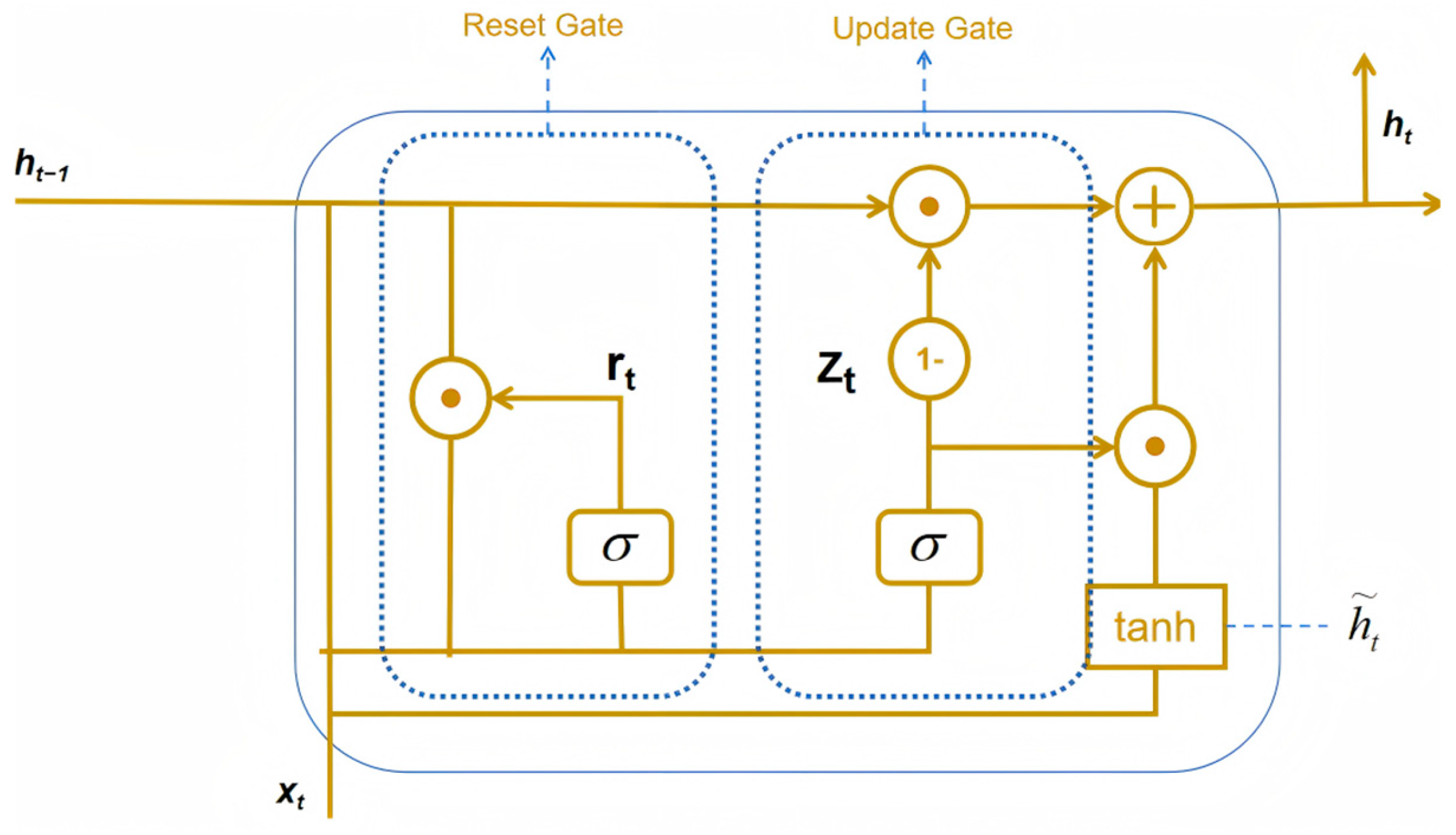
As shown in Figure 3, the GRU structure contains three main components: Reset Gate determines how to combine new input information with previous memory; Update Gate decides how much previous memory information needs to be retained; Candidate Hidden State calculates new candidate states based on current input and reset historical information. The forward propagation process of GRU can be represented by the following mathematical formulas:
Reset gate calculation:
r t = σ ( W r [ h t 1 , x t ] + b r )
Update gate calculation:
z t = σ ( W z [ h t 1 , x t ] + b z )
Candidate hidden state calculation:
h ~ t = tanh ( W h [ r t h t 1 , x t ] + b h )
Final hidden state calculation:
h t = ( 1 z t ) h t 1 + z t h ~ t
where: x t is the input vector at time t , h t is the hidden state at time t , r t is the reset gate output, z t is the update gate output, h ~ t is the candidate hidden state, W r , W z , W h are weight matrices, b r , b z , b h are bias vectors, σ is the sigmoid activation function, is the Hadamard product (element-wise multiplication), and [ , ] is the vector concatenation operation.
Residual connections: To address the gradient vanishing problem in deep networks, residual connections are added between dimension-matched layers. When input and output dimensions do not match, linear projection layers are used to align dimensions, ensuring the effectiveness of residual connections.
h t ( l ) = G R U ( l ) ( h t ( l 1 ) ) + F ( h t ( l 1 ) )
where: F (·) is the dimension projection function.
GRU demonstrates exceptional performance in runoff prediction, with its gating mechanism perfectly aligning with the characteristic requirements of hydrological time series [18]. GRU achieves selective memory and forgetting of historical information through update gates and reset gates: The update gate determines how much historical state information to retain, suitable for modeling long-term hydrological components like base flow; the reset gate controls the integration level between current input and historical information, effectively addressing the non-stationary characteristics of runoff processes.

3.2.3. Informer-GRU Network Construction

As shown in Figure 4, the Informer-GRU fusion model adopts a hierarchical progressive architecture design, organically combining Informer’s long sequence modeling capability with GRU’s temporal memory mechanism. The model overall adopts a four-layer progressive architecture:
(1) Input Embedding Layer
Converts original temporal data into high-dimensional feature representations through DataEmbedding, including parallel branches of data embedding and temporal feature embedding, providing rich semantic information for subsequent attention calculations.
(2) Informer Feature Extraction Layer
Consists of encoder-decoder structure, specifically handling long sequence dependencies and global temporal pattern recognition.
The encoder adopts a multi-layer EncoderLayer structure, each layer contains: ProbSparse self-attention mechanism, Feedforward network, Residual connection and layer normalization.
The decoder’s sequence generation: By combining the encoder’s output with partial future information, the decoder utilizes self-attention and cross-attention mechanisms to generate intermediate representations for prediction. The decoder input consists of both the labeled portion containing known sequences and the masked portion requiring prediction.
(3) Deep GRU Processing Layer
The multi-level GRU network is equipped with residual connection and self-attention mechanism for deep extraction of sequence features.
Attention enhancement mechanism: After adding a multi-head attention layer to the even-numbered GRU, the model can refocus on the important time steps in the sequence, establish long-distance temporal dependence, and enhance the model’s ability to recognize key patterns.
Residual connection and regularization: Each GRU is equipped with residual projection layer (to deal with dimension mismatch), layer normalization (to stabilize the training process) and Dropout mechanism (to prevent overfitting).
(4) Output Mapping Layer
Fully connected network that maps GRU output to final prediction results.
The Collaborative Mechanism Between Informer and GRU: Within the layered progressive architecture of Informer-GRU, the two modules achieve effective functional complementarity. The Informer handles global modeling by capturing dependencies between any positions in the sequence through attention mechanisms, excelling at processing long-term trends and periodic patterns. The GRU focuses on local refinement via gating mechanisms and sequential processing, enabling detailed characterization of short-term fluctuations and localized temporal features. This enhances the model’s comprehensive understanding of time series, thereby improving prediction accuracy. In terms of computational efficiency and training stability, the ProbSparse self-attention mechanism in Informer significantly reduces computational load and memory consumption when handling long sequences, allowing efficient processing of large-scale time series data. Meanwhile, the GRU effectively mitigates gradient disappearance and explosion issues inherent in traditional RNNs through its gating mechanism, ensuring stable model training across the hierarchical structure and preventing convergence failures caused by abnormal gradients. From the perspective of feature extraction and model adaptability, Informer’s multi-head self-attention mechanism and hierarchical architecture extract rich multi-scale features from time series. The GRU further filters and integrates these features through reset gates and update gates, enabling the model to better adapt to different types of time series data. This significantly enhances the model’s generalization capabilities and processing efficiency for complex time series data.

3.2.4. Forecasting Process

As shown in Figure 5, the complete workflow for daily runoff prediction in this study is illustrated. The process primarily involves: raw data → data cleaning → secondary decomposition → dataset construction → input into the Informer-GRU model for prediction → visualization of predicted results → SHAP analysis, along with GTO optimization, comparative experiments, and ablation tests.

3.3. Model Training and Optimization Methods

3.3.1. GTO Optimization Algorithm

The Gorilla Troops Optimizer (GTO) is a novel meta-heuristic optimization algorithm inspired by the social behavior and foraging strategies of gorilla groups [31]. The algorithm demonstrates excellent performance in both continuous and discrete optimization problems through balanced exploration-exploitation mechanisms, adaptive parameter adjustment strategies, and robust convergence characteristics [32].
GTO Algorithm Process Steps:
(1) Population Initialization
The initial population is randomly generated within the search space Ω = j = 1 D [ L j , U j ] :
X i , j ( 0 ) = L j + r a n d i , j × ( U j L j )
where D is the dimension number, L j and U j are the lower and upper bounds of the j -th parameter, and r a n d i , j U ( 0,1 ) .
(2) Fitness Evaluation
The comprehensive fitness function combines prediction accuracy, architecture quality, and model complexity:
F ( X i ) = w 1 R v a l 2 ( X i ) + w 2 Q a r c h ( X i ) w 3 P c o m p ( X i )
where R v a l 2 ( X i ) is the validation R-squared score, Q a r c h ( X i ) represents the architecture quality score, P c o m p ( X i ) denotes the complexity penalty, and the weight coefficients are set as w 1 = 1.0 , w 2 = 0.02 , a n d   w 3 = 0.1 .
(3) Adaptive Parameter Control
The inertia weight decreases linearly during the optimization process:
w ( t ) = w m a x t T m a x × ( w m a x w m i n )
The cognitive and social factors are dynamically adjusted:
c 1 ( t ) = c 1 , i n i t × exp α t T m a x , c 2 ( t ) = c 2 , i n i t × 1 + β t T m a x
where c 1 , i n i t = c 2 , i n i t = 2.0 , α = 2.0 , a n d   β = 1.0 .
(4) Exploration and Exploitation Mechanisms
The exploration probability decreases exponentially:
P e x p l o r e ( t ) = P e x p l o r e , 0 × exp γ t T m a x
where P e x p l o r e , 0 = 0.5 a n d   γ = 1.5 .
Exploration Phase: Position update follows:
X i n e w = X i ( t ) + ε i R i
where ε i N ( 0 , σ e x p l o r e 2 I ) and σ e x p l o r e = 0.1 .
Exploitation Phase: Individuals move toward the global best solution:
X i n e w = X i ( t ) + c 1 ( t ) r 1 ( X g b e s t X i ( t ) ) + δ i
where r 1 U ( 0,1 ) D and δ i N ( 0 , σ e x p l o i t 2 I ) with σ e x p l o i t = 0.05 .
(5) Genetic Operations
Crossover: Roulette wheel selection is employed for parent selection, followed by uniform crossover.
Mutation: The adaptive mutation probability is calculated as:
P m ( t ) = P m , m a x × 1 t T m a x 2
where P m , m a x = 0.3 .
(6) Population Update and Termination
Elite preservation strategy retains the top N e = 0.2 N individuals. The algorithm terminates when any of the following conditions is met: Maximum iteration limit reached; Fitness variance below threshold with consecutive stagnation; Population diversity falls below minimum threshold.
This study employs the Gorilla Troops Optimizer (GTO) for automatic hyperparameter search, achieving comprehensive optimization of the Informer-GRU model, including global optimization of model architecture parameters (hidden layer configuration, number of attention heads, etc.) and training parameters (learning rate, batch size, etc.).

3.3.2. Multi-Objective Loss Function Design

Traditional single loss functions (such as MSE) are difficult to comprehensively evaluate the quality of hydrological predictions. To comprehensively consider numerical accuracyand physical reasonableness, this study designs a multi-objective loss function. The total loss function consists of five parts: Mean Squared Error (MSE), Mean Absolute Error (MAE), Huber Loss, Nash-Sutcliffe Efficiency (NSE), and correlation [33,34]. The calculation formula is as follows:
L t o t a l = λ 1 L M S E + λ 2 L M A E + λ 3 L H u b e r + λ 4 L N S E + λ 5 L C o r r
(1) MSE Loss: L M S E = 1 N i = 1 N ( y i y ^ i ) 2
(2) MAE Loss: L M A E = 1 N i = 1 N | y i y ^ i |
(3) Huber Loss: L H u b e r = { 1 2 ( y i y ^ i ) 2 | y i y ^ i | δ δ | y i y ^ i | 1 2 δ 2 | y i y ^ i | > δ }
(4) NSE Loss: The Nash-Sutcliffe Efficiency (NSE) is a standard indicator for hydrological model evaluation, with a value range of ( , 1 ] , where values closer to 1 indicate better model performance. The NSE loss is defined as 1 minus the NSE value, ensuring the minimization objective of the loss function.
L N S E = 1 i = 1 N ( y i y ^ i ) 2 i = 1 N ( y i y ¯ ) 2
(5) Correlation Loss: L C o r r = 1 i = 1 N ( y i y ¯ ) ( y ^ i y ^ ¯ ) i = 1 N ( y i y ¯ ) 2 i = 1 N ( y ^ i y ^ ¯ ) 2
Where: y i represents the observed values; y ^ i represents the predicted values; y ¯ represents the mean of observed values; y ^ ¯ represents the mean of predicted values; N is the total number of samples; δ is the threshold parameter for Huber loss; λ 1 , λ 2 , λ 3 , λ 4 , λ 5 are the respective weight coefficients for each loss component.
The loss weights λ 1 λ 5 are also included as GTO optimization parameters, achieving adaptive configuration of the loss function.

3.3.3. Interpretability Methods

SHAP (SHapley Additive exPlanations) is a model interpretation method based on Shapley values from cooperative game theory, proposed by Lundberg and Lee in 2017. This method assigns an importance value to each feature of machine learning models to explain the contribution of individual predictions [35]. SHAP method is suitable for analyzing and interpreting complex relationships in neural network models, with larger Shapley values indicating greater importance of feature values to model prediction results [36].
For a cooperative game ( N , v ) , where N = 1,2 , . . . , n is the set of participants and v : 2 N R is the characteristic function, the Shapley value of participant i is defined as:
ϕ i ( v ) = S N i | S | ! ( n | S | 1 ) ! n ! [ v ( S i ) v ( S ) ]
where: S is the feature subset not containing feature i , | S | is the size of subset S , and v ( S i ) v ( S ) is the marginal contribution of feature i to coalition S .

3.4. Model Evaluation Metrics

This study adopts 5 evaluation metrics covering basic regression errors and hydrology-specific efficiency coefficients to comprehensively evaluate model performance, validating model prediction accuracy and hydrological adaptability from different dimensions, avoiding limitations of single metrics [37]. The evaluation indicators are as follows:
(1) The coefficient of determination (R2) measures goodness of fit:
R 2 = 1 ( y ^ y ) 2 ( y y ¯ ) 2
where values closer to 1 indicate better explanatory power.
(2) The Root Mean Square Error (RMSE) quantifies average prediction errors:
R M S E = 1 N ( y ^ y ) 2
where lower values indicating higher accuracy.
(3) The Mean Absolute Error (MAE) provides robust error measurement:
M A E = 1 n i = 1 n | y i y ^ i |
where being less sensitive to outliers than RMSE.
(4) The Nash-Sutcliffe Efficiency (NSE) evaluates hydrological model performance:
N S E = 1 ( y ^ y ) 2 ( y y ¯ ) 2
where values approaching 1 indicating excellent predictive capability.
(5) The Kling-Gupta Efficiency (KGE) provides comprehensive assessment:
K G E = 1 ( r 1 ) 2 + ( α 1 ) 2 + ( β 1 ) 2
where: r is the correlation, α is the standard deviation ratio, and β is the mean ratio.

4. Results Analysis

4.1. Data Preprocessing

The original runoff and precipitation data did not have any missing critical fields, with complete samples. Outlier detection and correction: 1641 outliers were detected using the IQR method (1569 from precipitation stations, 72 from runoff). Precipitation data were processed by setting negative values to zero and using statistical boundaries (3σ + 95th percentile replacement) to handle 504 outliers. Runoff data were processed using a combination of Hampel filter and EWMA smoothing to handle 72 outliers.

4.2. STL-CEEMDAN Secondary Decomposition

4.2.1. STL Decomposition

The STL decomposition of the runoff time series successfully separated the original time series into three independent components: trend, seasonal, and residual, providing high-quality feature inputs for subsequent deep learning modeling and CEEMDAN decomposition.
Characteristics and Hydrological Significance of STL Components (Figure 6):
(1)
Original Runoff Series: The series exhibits approximately nine complete cycles, indicating distinct inter-annual periodicity. Peak values show non-uniform distribution with inter-annual variations in intensity, where some years display significantly higher peaks than others. This pattern likely reflects differences in precipitation intensity and climate variability impacts across different years.
(2)
Trend Component: The trend component reveals long-term evolution patterns of the runoff series, manifesting as a nonlinear variation process. The first half primarily shows an ascending trend, potentially associated with factors such as reduced watershed vegetation and long-term precipitation increases. The latter half exhibits smooth curves with gradual long-term changes, possibly related to stable underlying surface conditions and consistent precipitation patterns. The final segment shows a declining trend, potentially linked to increased watershed water consumption and ecological restoration activities.
(3)
Seasonal Component: Displays regular oscillations with annual periodicity (365 days), with peaks concentrated during the rainy season (e.g., summer) and troughs during the dry season (e.g., winter). The amplitude variations of the seasonal component closely resemble those of the original series, indicating that seasonal variations are the dominant factor in runoff changes. This characteristic aligns with hydrological systems being significantly influenced by seasonal precipitation patterns.
(4)
Residual Component: Exhibits periodic fluctuation characteristics, indicating that the residual contains information from short-term meteorological events causing runoff fluctuations, irregular hydrological processes, extreme event information, measurement noise, and other random disturbances. This provides an information foundation for CEEMDAN decomposition.
Figure 6. STL time series decomposition results.
Water 17 02775 g006

4.2.2. CEEMDAN Decomposition

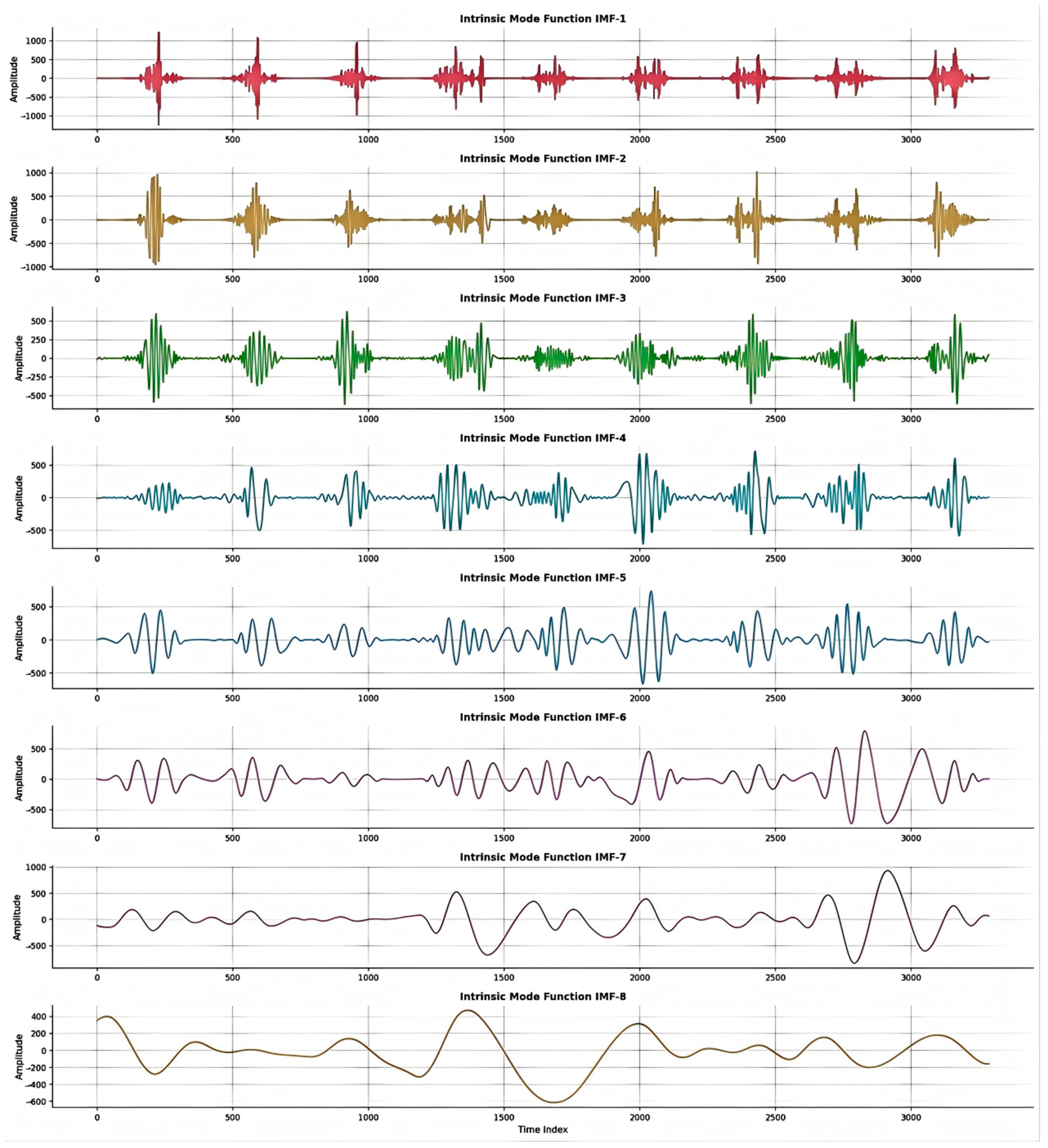
IMF Component Characteristics (Figure 7): The CEEMDAN algorithm successfully decomposed the STL residual signal into eight components (IMF1–IMF8), achieving fine-scale decomposition across the full frequency spectrum of the residual signal. IMF-1 to IMF-3 display pronounced high-frequency periodic oscillations, potentially corresponding to measurement noise, short-term meteorological disturbances, or high-frequency responses of data acquisition systems. IMF-4 to IMF-6 show relatively distinct medium-frequency periodic oscillations, possibly reflecting weekly to monthly hydrological process variations, such as short-term impacts of precipitation events and daily variations in evapotranspiration. IMF-7 to IMF-8 exhibit obvious low-frequency fluctuations with less distinct periodic oscillations, potentially corresponding to irregular hydrological processes such as groundwater recharge variations and snowmelt runoff patterns.

4.3. Dataset Preparation and Splitting

After data cleaning and STL-CEEMDAN dual decomposition, the final dataset integrated 6 precipitation series from monitoring stations, 3 STL components, and 8 CEEMDAN features (IMF1–8), totaling 17 features as input variables. The dataset was partitioned using a three-way split approach: 70% training + 15% validation + 15% testing. The training set spans from 1 January 2015, to 12 April 2021 (2300 days); the validation set covers 13 April 2021, to 19 July 2022 (493 days); and the testing set extends from 20 July 2022, to 31 December 2023 (494 days).

4.4. GTO Optimization Results

The GTO optimization in this study mainly includes two stages: dataset parameter optimization and deep learning model optimization. Deep learning model optimization includes model architecture parameter optimization, training hyperparameter optimization, and multi-objective loss function weight optimization. The specific optimization results are shown in Table 1.
The GTO optimization yielded notable parameter adjustments across four categories. Dataset parameters showed minor increases in window size (24→26) and label length (12→13). Model architecture optimization produced an irregular GRU configuration [502, 303, 184, 393, 458, 169] for enhanced multi-scale feature capture, while the Transformer dimension increased substantially (185→350). Training hyperparameters were refined with a modest learning rate increase (0.000063→0.000095), reduced batch size (43→39), and fewer epochs (38→33), indicating improved convergence efficiency. Loss function weights underwent significant rebalancing, with MAE weight increasing from 0.2413 to 0.3624 and NSE weight rising from 0.1417 to 0.2404, while Huber loss weight decreased from 0.2880 to 0.2089, emphasizing absolute error minimization and hydrological performance metrics.

4.5. Prediction Results Analysis

The model designed in this study shows excellent prediction results on the test set with R2 = 0.947 and NSE = 0.947, both close to 1, indicating excellent model ability to explain runoff sequence variation and capture core patterns of runoff changes. Although test set indicators are slightly lower than validation set, this represents normal fluctuation in the model’s adaptation to unknown data during generalization, while overall maintaining high fitting levels, proving the model’s stable trend fitting capability. While RMSE and MAE error indicators show slight increases on the test set due to uncertainties in predicting unknown data, the overall values remain in low ranges, indicating that prediction values and true values have controllable absolute deviations, and the model can output reliable runoff prediction results in practical applications. The KGE indicator even improves on the test set to 0.958, indicating good model performance in matching runoff sequence central tendency, dispersion, and fluctuation correlation. The specific results are shown in Table 2.

4.6. Comparative Experiment Results Analysis

To validate the effectiveness of the combined model, this section designed a runoff prediction comparison experiment. Various models including LSTM, GRU, Transformer, Informer, and CNN-LSTM were employed. For ease of comparison, all inputs matched those of our research model, and hyperparameters were optimized using GTO. Through performance metric comparisons, time series prediction curves, and scatter plot distribution analysis, we investigated the performance of different models in runoff prediction within the Liyuan Basin.
Table 3 demonstrates that the STL-CEEMDAN+GTO-Informer-GRU Model (My Model) outperforms other models across all metrics: achieving an R2 of 0.946936 and NSE of 0.958182 (significantly outperforming alternative models), highlighting its improved explanatory power and simulation accuracy for runoff sequences. The model also shows excellent prediction precision, with RMSE at 271.51 and MAE at 186.78. While LSTM and GRU performed relatively well among other models, they still lag significantly behind the My Model.
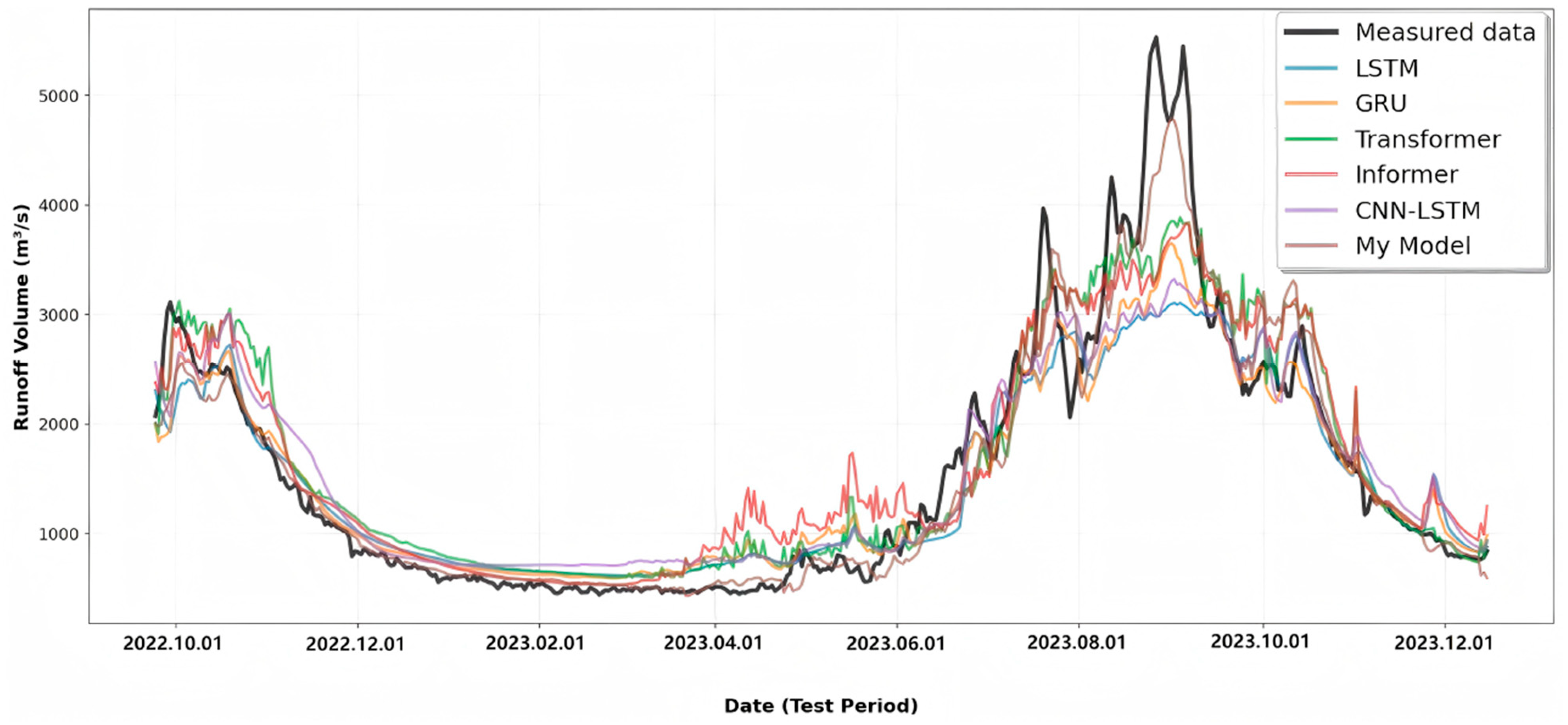
As shown in Figure 8, there are discrepancies between the predicted trends of different models and the true values (True Values). Traditional deep learning models such as LSTM and GRU can capture general runoff trends, but their prediction curves deviate significantly from actual values during peak and trough periods. For instance, during peak runoff periods (some nodes in 2023), models like LSTM and Transformer produced predictions lower than actual values, indicating limited capability in simulating extreme runoff scenarios. In contrast, My Model’s prediction curve closely matched the true values across different phases of the runoff sequence: the decaying phase (October 2022 to May 2023), growth phase (May 2023 to September 2023), and post-decay phase (after September 2023). Particularly during peak runoff periods (August–September 2023), the predicted curve accurately captured the fluctuation patterns of the observed values, demonstrating excellent predictive performance.
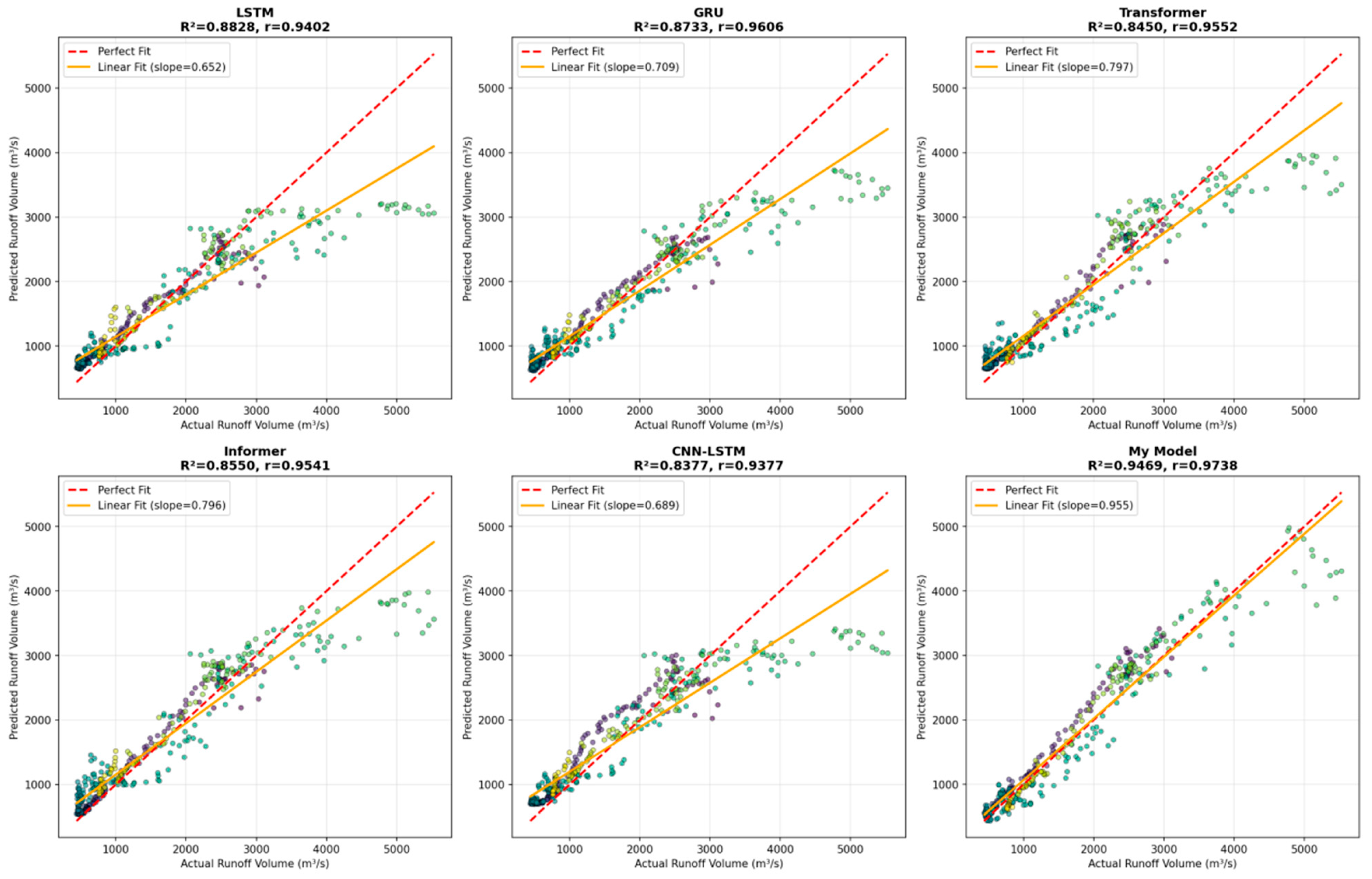
As shown in Figure 9, the ideal prediction demonstrates a scattered distribution near the 1:1 dashed line. The CNN-LSTM model exhibits high dispersion with a R2 value of 0.8377, showing the weakest linear correlation between predictions and actual values. Although models like LSTM, GRU, and Transformer show some deviation from the dashed line, Transformer demonstrates better alignment R2 with a 0.8450 value, indicating discrepancies between predicted and actual results. My Model’s predictions closely follow the 1:1 dashed line with R2 reaching 0.9469, demonstrating strong linear relationships between predictions and actual values, ensuring high reliability and more precise runoff numerical mapping.

4.7. Ablation Experiment Results Analysis

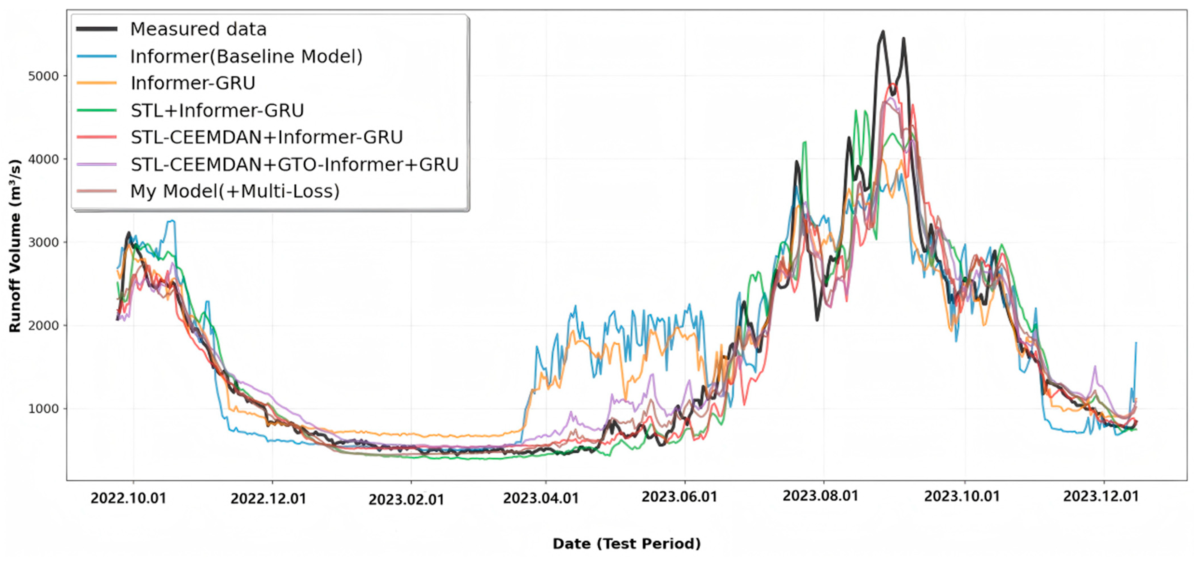
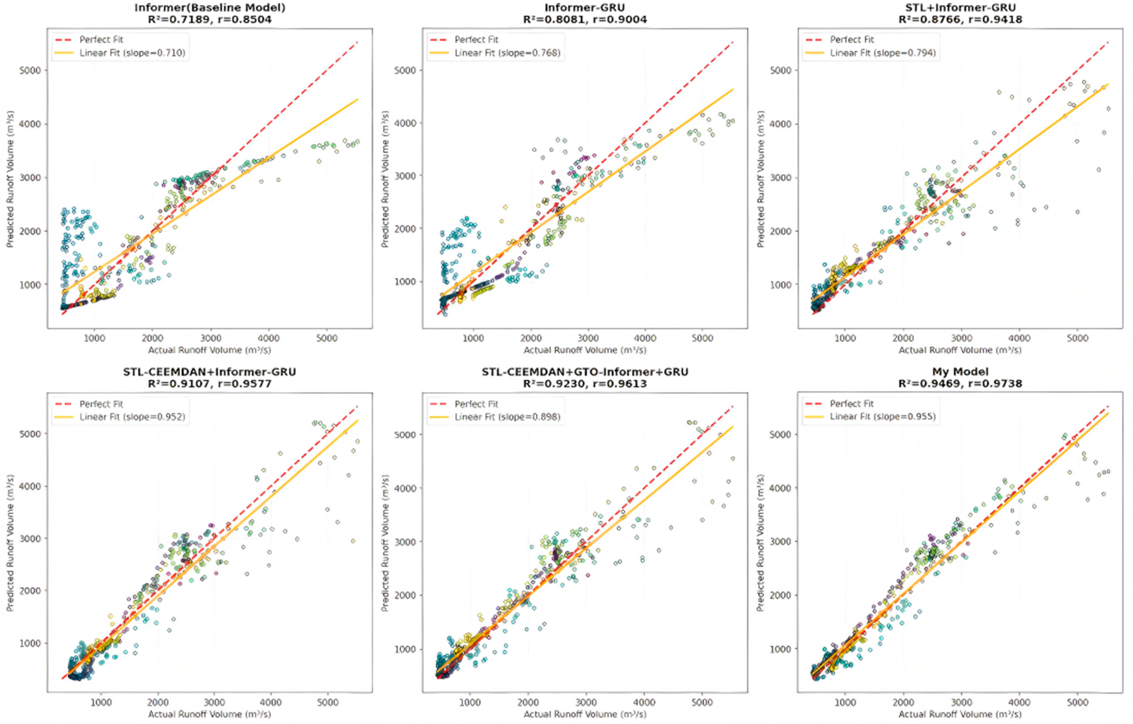
To further demonstrate the synergistic effects of model structure and components on prediction accuracy improvement, this section conducts ablation experiments by progressively introducing GRU, STL, CEEMDAN, GTO, and multi-objective loss function to the Informer baseline model. The analysis examines model performance through performance metrics comparison, time-series prediction curves, and scatter plot distribution analysis, providing deep insights into the gain pathways of each module for prediction performance and revealing the intrinsic mechanisms of model accuracy enhancement.
As clearly shown in Table 4, with Informer as the baseline, each module demonstrates stepwise optimization of performance metrics. After introducing GRU, R2 improved by 12.41% and RMSE decreased to 516.33. In the Liyuan watershed, runoff is driven by multiple processes including precipitation and infiltration, exhibiting complex temporal dynamics. The gating mechanisms of GRU (update gate and reset gate) enhanced the extraction capability for long-term and short-term dependencies in runoff sequences. Through adaptive forgetting of historical information and focusing on critical periods (such as flood response during rainy seasons), GRU compensated for Informer’s insufficient capture of high-frequency temporal fluctuations, preliminarily enhancing the model’s fitting accuracy for runoff dynamic changes.
After adding STL, R2 improved by 8.48%. In the Liyuan watershed, runoff exhibits significant seasonality driven by monsoon climate (such as rainy/dry season cycles). STL decomposition enables the model to separately learn periodic fluctuations (such as monthly runoff abundance patterns) and long-term trends (such as gradual impacts of underlying surface changes), resolving Informer’s “confusion in mixed signal learning” and improving explanatory power for regular runoff components.
CEEMDAN decomposition of residuals provided certain performance improvements by mining subtle fluctuations and supplementing the model’s identification of non-stationary, nonlinear hydrological signals. After adding GTO and multi-objective loss function, R2 improved by 1.34% and 2.59%, respectively. The multi-objective loss function balanced multiple optimization targets, addressing the problem of single loss functions (such as MSE) focusing only on numerical errors while ignoring the rationality of hydrological processes.
From Figure 10, it is evident that each module progressively enhanced the fitting capability for runoff mutations, periodic fluctuations, and trend continuation. Informer showed a severe lag in predicting flood season peaks in 2023 (such as June–August 2023). After adding GRU, although peak trends could be captured, amplitude deviations remained large. After adding CEEMDAN, the model could accurately identify precipitation-runoff mutation correlations (such as steep runoff rises caused by short-term heavy rainfall), with significantly improved curve fitting to actual values. STL-CEEMDAN+GTO-Informer-GRU Model (My Model) essentially reproduced the “steep rise-gradual decline” process of peaks, validating the adaptability of multi-objective functions to extreme hydrological events. Before STL introduction, the model’s identification of seasonal cycles (such as dry periods from December 2023 to February 2024, and wet periods from June to August 2024) was unclear. After introducing STL, curves clearly showed the annual “wet-dry-wet” cycle, demonstrating STL’s decoupling effect on seasonal signals. MyModel further enhanced small fluctuations within cycles (such as minor baseflow changes during dry periods), reflecting the synergistic capability of multiple modules for fine-grained periodic fitting.
From Figure 11, it is apparent that module stacking transformed scatter points from dispersed distribution to dense alignment with the 1:1 line, reflecting progressive improvement in prediction reliability. Baseline Informer scatter points were far from the diagonal line with extremely high dispersion in high-value regions (runoff peaks). After adding GRU and STL, scatter points converged toward the diagonal line, but deviations remained in medium-low value regions (dry periods), reflecting that the GRU-STL combination could capture temporal and periodic features but had insufficient error control for low flows. Further addition of CEEMDAN and GTO increased scatter point density and reduced medium-low value region deviations, as CEEMDAN’s residual mining supplemented low-flow fluctuation information, and GTO optimization reduced systematic bias. Finally, MyModel scatter points almost perfectly aligned with the diagonal line, with further reduced dispersion in high/medium/low value regions, benefiting from multi-objective loss function joint optimization that ensured balanced prediction errors across all flow intervals (wet/dry periods).
Through comparative experiments with traditional models such as LSTM and GRU, and ablation experiments exploring individual or combined effects of each module, MyModel demonstrated significant advantages. The “signal decomposition to global optimization” framework constructed in this study provides moderate interpretation of deep learning “black boxes,” improving the interpretability of deep learning models in hydrological applications.

4.8. Model Interpretability Analysis

To further analyze the decision-making logic of the model in runoff prediction tasks, this study employed the SHAP (SHapley Additive exPlanations) method for detailed quantitative analysis of feature importance, aiming to uncover the intrinsic mechanisms of model decision-making.
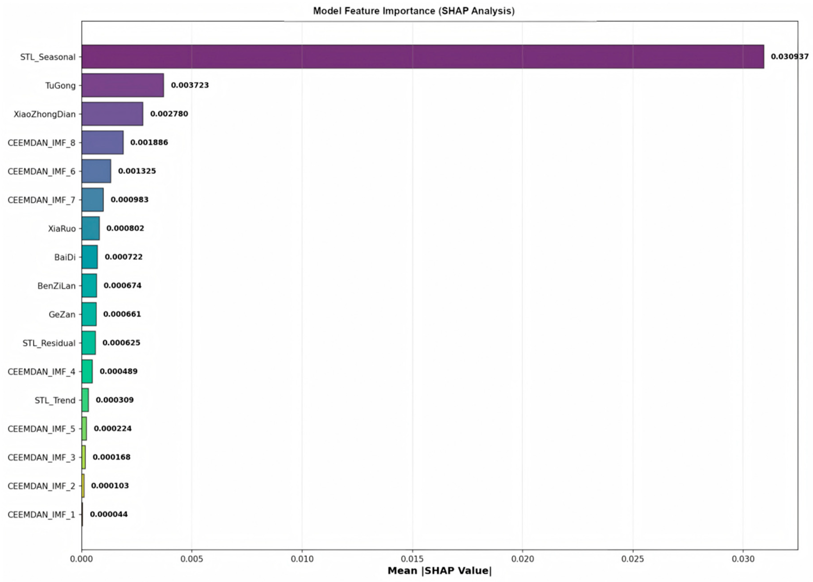
As shown in Figure 12, STL_Seasonal emerges as the core feature influencing model output with an average SHAP value of 0.03937. In the hydrological cycle, runoff in the Liyuan watershed is driven by factors such as seasonal precipitation distribution and periodic temperature variations, exhibiting significant seasonal patterns. The high contribution value of STL_Seasonal intuitively confirms the model’s precise capture of seasonal components in runoff series, indicating that the model can align with the periodic nature of hydrological processes and use seasonal signals as the core basis for prediction. This highly matches the natural mechanisms of watershed runoff formation and serves as key support for accurate model prediction.
In comparison, STL_Residual and STL_Trend show relatively lower contributions. STL_Trend reflects long-term trends in the series; during the study period, the watershed may have been influenced by gradual climate change and relatively stable underlying surface conditions, resulting in less prominent long-term trend characteristics in runoff, which limits its explanatory power for prediction. STL_Residual contains random disturbances and information not explained by trend and seasonal components. Due to their strong randomness and difficulty in pattern recognition, such information naturally contributes less directly to prediction, which also indicates that the model focuses on more regular features for prediction.
TuGong (0.003723) and XiaoZhongDian (0.002780) rank highly in feature contributions, highlighting the value of local hydrological station data. Local stations directly observe precipitation, water levels, and other information within the watershed, serving as direct inputs for runoff formation. Their high contributions are related to watershed hydrological response characteristics, as local processes such as precipitation infiltration and runoff generation are quickly reflected in runoff changes. The model identifies the direct driving effect of these local features on runoff. The decreasing average SHAP values of other precipitation stations are closely related to the spatial distribution of watershed rainfall and topographic conditions. The Liyuan watershed has complex terrain, with rainfall affected by topographic lifting and blocking, resulting in strong spatial heterogeneity. Stations farther from the runoff monitoring area contribute less to target watershed runoff due to topographic attenuation and confluence losses, reflecting the model’s effective identification of watershed hydrology-topography coupling relationships.
Various IMF components from CEEMDAN decomposition (such as IMF_6, IMF_7, IMF_8), although less important than STL_Seasonal, still participate in model decision-making. Through CEEMDAN decomposition, residuals are decomposed into different frequency fluctuation components, covering short-term and medium-term disturbances, supplementing runoff variation details, and reflecting the influence of factors such as short-term heavy rainfall and medium-term climate fluctuations on runoff within the watershed. This indicates that runoff changes in the Liyuan watershed result from seasonal dominance in the original series, combined with multi-scale fluctuation synergistic driving. The model integrates multi-dimensional features to construct a more comprehensive runoff prediction logic.
In summary, SHAP analysis validates the model’s advantages in capturing seasonal signals and identifying local hydrological features from the feature contribution perspective. It clearly deconstructs the runoff prediction mechanism under multi-variable driving, where seasonal components dominate while local stations and multi-scale components work synergistically, providing quantitative support for the physical interpretability and credibility of model prediction results.

5. Discussion

5.1. Model Performance Comparison with Existing Studies

The proposed STL-CEEMDAN+GTO-Informer-GRU model demonstrates substantial improvements over existing approaches in hydrological runoff prediction, achieving R2 = 0.9469 and NSE = 0.9469 compared to Wilbrand K et al. [11] (R2 = 0.83 with LSTM) He et al. [19] (R2 = 0.93 with SD-GRU) and Wang et al. [20] (NSE = 0.72 with STL-LightGBM). These improvements stem from three key methodological advantages: our dual decomposition strategy (STL-CEEMDAN) provides more comprehensive feature extraction than single decomposition methods by separating deterministic components before applying adaptive noise-enhanced decomposition to residuals; the Informer-GRU hybrid architecture reduces computational complexity from O(L2) to O(L log L) while capturing both long-range dependencies through ProbSparse attention and local temporal features through gating mechanisms; and GTO optimization ensures optimal model configuration across the complex parameter space, eliminating the limitations of manual parameter tuning employed in previous studies.

5.2. Applicability Analysis and Generalization Potential

The proposed methodology’s transferability across different watershed scales and climatic conditions requires careful consideration of several key factors. For small-scale watersheds, particularly mountain streams with rapid meteorological responses, the high-frequency IMF components (IMF1-IMF3) would likely assume greater predictive importance due to reduced buffering capacity and faster concentration times, necessitating modifications such as shorter temporal windows (12–18 days) and integration of precipitation intensity metrics alongside soil moisture indices. In different climatic regions, the methodology faces varying challenges: arid regions would require incorporation of evapotranspiration data and recalibrated decomposition parameters due to minimal baseflow contributions; snow-dominated regions would need extended input sequences with temperature-based snowmelt indicators, though CEEMDAN’s effectiveness for nonlinear snowmelt processes requires validation; tropical regions with uniform seasonal patterns might show reduced STL seasonal variability, shifting emphasis toward residual-based IMF components. For larger basin systems, spatial heterogeneity challenges emerge that could be addressed through sub-basin-specific decomposition with aggregation, spatially distributed input data, and routing delay incorporation, though the GTO optimization process would require careful parallelization to maintain computational efficiency across multiple sub-models while leveraging the Informer architecture’s scalability advantages over traditional RNN approaches.

5.3. Implications for Water Resource Management in Yunnan Region

The developed methodology provides significant practical value for water resource management in the Yunnan region, addressing unique challenges from plateau mountain geography, monsoon climate variability, and complex topography through high-accuracy daily runoff predictions (R2 = 0.9469, KGE = 0.9582). The model’s 13-day forecast horizon enables proactive reservoir water release strategies during seasonal transitions, optimizing flood control and water supply objectives, while its superior performance during peak flow periods (demonstrated in August–September 2023 predictions) proves particularly valuable for flood management in downstream urban and agricultural zones. Agricultural water management benefits from the model’s seasonal pattern recognition capability, with SHAP analysis revealing STL_Seasonal as the dominant feature (average SHAP value = 0.0394), confirming alignment with crop irrigation cycles and enabling precise irrigation scheduling and water allocation planning across diverse agricultural zones. The methodology’s integration of multiple precipitation stations addresses spatial variability characteristic of mountain watersheds, and while current gauge distribution concentrates in lower elevation areas, the model framework remains adaptable to incorporate additional remote sensing precipitation products (such as GPM IMERG or CHIRPS datasets) for improved spatial coverage and prediction accuracy in data-sparse upper watershed areas.

5.4. Methodological Limitations and Future Research Directions

Despite the promising results, several limitations warrant acknowledgment while pointing toward future research opportunities. The spatial distribution of precipitation gauges concentrated in the lower watershed may introduce bias in representing orographic precipitation patterns, though the temporal decomposition approach partially mitigates this through pattern extraction rather than spatial interpolation. The model shows systematic underestimation during extreme flow events, a common limitation in data-driven approaches that suggests incorporating physical constraints or extreme value theory. Additionally, while the Informer architecture reduces computational complexity, the GTO optimization process remains resource-intensive, potentially limiting real-time applications, and the model’s reliance on historical patterns assumes stationarity that may not hold under changing climate conditions. Future research should focus on integrating remote sensing data (satellite precipitation, soil moisture, vegetation indices) to address spatial limitations, developing physics-informed neural network variants to improve extreme event prediction through water and energy balance constraints, implementing ensemble modeling approaches for uncertainty quantification, exploring transfer learning for ungauged basin applications within the Yunnan region, and establishing real-time model updating mechanisms with recursive parameter adjustment to address non-stationarity concerns in rapidly changing environments.

6. Conclusions

This study addresses the challenges of high data complexity and insufficient generalization capability of single models in hydrological runoff prediction by proposing a deep learning prediction framework that integrates STL-CEEMDAN dual decomposition, Informer-GRU hybrid architecture, GTO optimization, and multi-objective loss function. The main conclusions are as follows:
(1)
Dual decomposition strategy significantly enhances feature extraction capability: The STL-CEEMDAN hierarchical decomposition framework achieves precise separation of multi-scale features in runoff data. STL effectively extracts deterministic components such as trend and seasonality, while CEEMDAN further decomposes residuals into IMF components of different frequencies, filtering high-frequency noise while preserving critical information such as extreme events and short-term fluctuations. Compared to single decomposition methods, dual decomposition enhances the physical interpretability of input features, providing more targeted inputs for subsequent model learning.
(2)
Informer-GRU hybrid architecture enables synergistic modeling of global and local features: By integrating Informer’s ProbSparse attention mechanism with GRU’s gating memory mechanism, the model simultaneously captures long-range dependencies in runoff sequences (such as inter-annual trends) and local temporal features (such as short-term flood fluctuations). This synergy enhances the model’s capability to fit complex hydrological processes.
(3)
GTO optimization and multi-objective loss function improve model performance and robustness: The GTO algorithm achieves global optimization of model architectural parameters (such as hidden layer numbers and attention heads) and training hyperparameters (such as learning rate and batch size), avoiding the problem of traditional parameter tuning falling into local optima. The multi-objective loss function comprehensively considers metrics such as MSE, MAE, and NSE, balancing numerical accuracy with the physical rationality of hydrological processes, making the model more robust in runoff prediction.
(4)
Case validation demonstrates excellent prediction accuracy and generalization capability: In daily runoff prediction for the Liyuan watershed from 2015–2023, the model achieved R2 and NSE values of 0.9469 and KGE of 0.9582 on the test set, significantly outperforming comparative models such as LSTM, GRU, and Transformer. Time-series curve and scatter plot analyses show that the model can accurately track runoff peaks, valleys, and seasonal variations, with particularly smaller prediction deviations during extreme flood periods. Ablation experiments confirm that the cumulative contribution of key components such as dual decomposition and GTO optimization improves model performance by 31.72% compared to the baseline Informer.
(5)
Feature importance analysis reveals prediction decision mechanisms: SHAP analysis indicates that seasonal components extracted by STL are the core features affecting prediction (average SHAP value of 0.0394), reflecting the essential nature of watershed runoff being driven by seasonal precipitation. Local precipitation stations (such as TuGong station) and medium-low frequency IMF components contribute significantly to short-term fluctuation prediction, validating the model’s effective identification of hydrological process driving factors.

Author Contributions

Conceptualization, A.H.; Methodology, H.Y.; Software, H.T.; Validation, H.Y.; Formal analysis, A.H.; Investigation, W.Z.; Resources, Y.W.; Data curation, Y.W.; Writing—original draft, H.Y.; Visualization, H.Y. and L.D.; Supervision, Y.W.; Project administration, Y.M.; Funding acquisition, Y.M. All authors have read and agreed to the published version of the manuscript.

Funding

This research was funded by the Science and Technology Project of China Southern Power Grid Yunnan Power Grid Co., Ltd., grant number YNKJXM20222329.

Data Availability Statement

The data used in this study are not publicly available due to confidentiality agreements and institutional restrictions. Interested researchers may contact the corresponding author for limited access under appropriate conditions.

Conflicts of Interest

Author Yi Ma and Yifan Wang are being employed by the company Electric Power Research Institute, Yunnan Power Grid Co, Ltd., China Southern Power Grid. The remaining authors declare that the research was conducted in the absence of any commercial or financial relationships that could be construed as apotential conflict of interest.

References

  1. Solaimani, K. Rainfall-runoff prediction based on artificial neural network (a case study: Jarahi watershed). Am.-Eurasian J. Agric. Environ. Sci. 2009, 5, 856–865. [Google Scholar]
  2. Li, F.F.; Cao, H.; Hao, C.F.; Qiu, J. Daily Streamflow Forecasting Based on Flow Pattern Recognition. Water Resour. Manag. 2021, 35, 4601–4620. [Google Scholar] [CrossRef]
  3. Wu, J.; Wang, Z.; Dong, J.; Cui, X.; Tao, S.; Chen, X. Robust runoff prediction with explainable artificial intelligence and meteorological variables from deep learning ensemble model. Water Resour. Res. 2023, 59, e2023WR035676. [Google Scholar] [CrossRef]
  4. Mao, G.; Wang, M.; Liu, J.; Wang, Z.; Wang, K.; Meng, Y.; Zhong, R.; Wang, H.; Li, Y. Comprehensive comparison of artificial neural networks and long short-term memory networks for rainfall-runoff simulation. Phys. Chem. Earth Parts a/b/c 2021, 123, 103026. [Google Scholar] [CrossRef]
  5. Han, H.; Morrison, R.R. Improved runoff forecasting performance through error predictions using a deep-learning approach. J. Hydrol. 2022, 608, 127653. [Google Scholar] [CrossRef]
  6. Lei, X.H.; Wang, H.; Yang, M.X.; Gui, Z.L. Research Progress on Meteorological Hydrological Forecasting under Changing Environments. J. Hydraul. Eng. 2018, 49, 9–18. (In Chinese) [Google Scholar]
  7. Zhu, S.; Zhou, J.; Ye, L.; Meng, C. Streamflow estimation by support vector machine coupled with different methods of time series decomposition in the upper reaches of Yangtze River, China. Environ. Earth Sci. 2016, 75, 531. [Google Scholar] [CrossRef]
  8. Xu, Y.; Hu, C.; Wu, Q.; Li, Z.; Jian, S.; Chen, Y. Application of temporal convolutional network for flood forecasting. Hydrol. Res. 2021, 52, 1455–1468. [Google Scholar] [CrossRef]
  9. Yin, H.; Zhu, W.; Zhang, X.; Xing, Y.; Xia, R.; Liu, J.; Zhang, Y. Runoff predictions in new-gauged basins using two transformer-based models. J. Hydrol. 2023, 622, 129684. [Google Scholar] [CrossRef]
  10. Zhou, J.; Peng, T.; Zhang, C.; Sun, N. Data pre-analysis and ensemble of various artificial neural networks for monthly streamflow for ecasting. Water 2018, 10, 628. [Google Scholar] [CrossRef]
  11. Wilbrand, K.; Taormina, R.; ten Veldhuis, M.-C.; Visser, M.; Hrachowitz, M.; Nuttall, J.; Dahm, R. Predicting streamflow with LSTM networks using global datasets. Front. Water 2023, 5, 1166124. [Google Scholar] [CrossRef]
  12. Clark, S.R.; Lerat, J.; Perraud, J.-M.; Fitch, P. Deep learning for monthly rainfall–runoff modelling: A large-sample comparison with conceptual models across Australia. Hydrol. Earth Syst. Sci. 2024, 28, 1191–1213. [Google Scholar] [CrossRef]
  13. Wang, F.; Mu, J.; Zhang, C.; Wang, W.; Bi, W.; Lin, W.; Zhang, D. Deep Learning Model for Real-Time Flood Forecasting in Fast-Flowing Watershed. J. Flood Risk Manag. 2025, 18, e70036. [Google Scholar] [CrossRef]
  14. Xu, D.M.; Li, Z.; Wang, W.C.; Hong, Y.H.; Gu, M.; Hu, X.X.; Wang, J. WaveTransTimesNet: An enhanced deep learning monthly runoff prediction model based on wavelet transform and transformer architecture. Stoch. Environ. Res. Risk Assess. 2025, 39, 883–910. [Google Scholar] [CrossRef]
  15. Jia, S.; Wang, X.; Xu, Y.J.; Liu, Z.; Mao, B. A New Data-Driven Model to Predict Monthly Runoff at Watershed Scale: Insights from Deep Learning Method Applied in Data-Driven Model. Water Resour. Manag. 2024, 38, 5179–5194. [Google Scholar] [CrossRef]
  16. Wang, S.; Wang, W.; Zhao, G. A novel deep learning rainfall–runoff model based on Transformer combined with base flow separation. Hydrol. Res. 2024, 55, 576–594. [Google Scholar] [CrossRef]
  17. Zhang, X.; Wang, R.; Wang, W.; Zheng, Q.; Ma, R.; Tang, R.; Wang, Y. Runoff prediction using combined machine learning models and signal decomposition. J. Water Clim. Change 2025, 16, 230–247. [Google Scholar] [CrossRef]
  18. He, F.; Wan, Q.; Wang, Y.; Wu, J.; Zhang, X.; Feng, Y. Daily Runoff Prediction with a Seasonal Decomposition-Based Deep GRU Method. Water 2024, 16, 618. [Google Scholar] [CrossRef]
  19. Wang, S.; Yang, K.; Peng, H. Using a seasonal and trend decomposition algorithm to improve machine learning prediction of inflow from the Yellow River, China, into the sea. Front. Mar. Sci. 2025, 12, 1540912. [Google Scholar] [CrossRef]
  20. Aerts, J.C.J.H. A Review of Cost Estimates for Flood Adaptation. Water 2018, 10, 1646. [Google Scholar] [CrossRef]
  21. Yu, L.; Wang, X.; Wang, J. An Adaptive Rolling Runoff Forecasting Framework Based on Decomposition Methods. Water Resour. Manag. 2025, 1–24. [Google Scholar] [CrossRef]
  22. Shiri, F.M.; Perumal, T.; Mustapha, N.; Mohamed, R. A Comprehensive Overview and Comparative Analysis on Deep Learning Models. J. Artif. Intell. 2024, 6, 301–360. [Google Scholar] [CrossRef]
  23. Roy, S.; Mehera, R.; Pal, R.K.; Bandyopadhyay, S.K. Hyperparameter optimization for deep neural network models: A comprehensive study on methods and techniques. Innov. Syst. Softw. Eng. 2025, 21, 789–800. [Google Scholar] [CrossRef]
  24. Chen, H.; Kang, L.; Zhou, L.; Zhang, W.; Wen, Y.; Ye, J.; Qin, R. Hybrid multi-module for short-term forecasting of river runoff considering spatio-temporal features. Hydrol. Res. 2025, 56, 60–73. [Google Scholar] [CrossRef]
  25. Cleveland, R.B.; Cleveland, W.S.; McRae, J.E.; Terpenning, I. STL: A seasonal-trend decomposition. J. Off. Stat. 1990, 6, 3–73. [Google Scholar]
  26. Torres, M.E.; Colominas, M.A.; Schlotthauer, G.; Flandrin, P. A complete ensemble empirical mode decomposition with adaptive noise. In Proceedings of the 2011 IEEE International Conference on Acoustics, Speech and Signal Processing (ICASSP), Prague, Czech Republic, 22–27 May 2011; IEEE: Piscataway, NJ, USA, 2011; pp. 4144–4147. [Google Scholar] [CrossRef]
  27. Ma, X.; Wang, R.; Zhang, Y.; Jiang, C.; Abbas, H. A name disambiguation module for intelligent robotic consultant in industrial internet of things. Mech. Syst. Signal Process. 2020, 136, 106413. [Google Scholar] [CrossRef]
  28. Zhou, H.; Zhang, S.; Peng, J.; Zhang, S.; Li, J.; Xiong, H.; Zhang, W. Informer: Beyond Efficient Transformer for Long Sequence Time-Series Forecasting. In Proceedings of the AAAI Conference on Artificial Intelligence, Virtual, 2–9 February 2021; Volume 35, pp. 11106–11115. [Google Scholar] [CrossRef]
  29. Zhu, S.; Wang, Z.; Zhang, W.; Yang, J. Application of the ResNet-Transformer Model for Runoff Prediction Based on Multi-source Data Fusion. Water Resour. Manag. 2025. [Google Scholar] [CrossRef]
  30. Cho, K.; Van Merriënboer, B.; Gulcehre, C.; Bahdanau, D.; Bougares, F.; Schwenk, H.; Bengio, Y. Learning phrase representations using RNN encoder-decoder for statistical machine translation. arXiv 2014, arXiv:1406.1078. [Google Scholar] [CrossRef]
  31. Abdollahzadeh, B.; Soleimanian Gharehchopogh, F.; Mirjalili, S. Artificial gorilla troops optimizer: A new nature-inspired metaheuristic algorithm for global optimization problems. Int. J. Intell. Syst. 2021, 36, 5887–5958. [Google Scholar] [CrossRef]
  32. Hussien, A.G.; Bouaouda, A.; Alzaqebah, A.; Kumar, S.; Hu, G.; Jia, H. An in-depth survey of the artificial gorilla troops optimizer: Outcomes, variations, and applications. Artif. Intell. Rev. 2024, 57, 246. [Google Scholar] [CrossRef]
  33. Li, Q.; Ishidaira, H.; Bastola, S.; Magome, J. Intercomparison of Hydrological Modeling Performance with Multi-Objective Optimization Algorithm in Different Climates. Annu. J. Hydraul. Eng. JSCE 2009, 53, 19–24. [Google Scholar]
  34. Huo, J.; Liu, L. Evaluation method of multiobjective functions’ combination and its application in hydrological model evaluation. Comput. Intell. Neurosci. 2020, 2020, 8594727. [Google Scholar] [CrossRef]
  35. Lundberg, S.M.; Lee, S.I. A unified approach to interpreting model predictions. Adv. Neural Inf. Process. Syst. 2017, 30, 4765–4774. Available online: https://proceedings.neurips.cc/paper/2017/hash/8a20a8621978632d76c43dfd28b67767-Abstract.html (accessed on 30 August 2025).
  36. Bhargava, D.; Gupta, L.K. Explainable AI in Neural Networks Using Shapley Values. In Biomedical Data Analysis and Processing Using Explainable (XAI) and Responsive Artificial Intelligence (RAI); Khamparia, A., Gupta, D., Khanna, A., Balas, V.E., Eds.; Intelligent Systems Reference Library; Springer: Singapore, 2022; Volume 222. [Google Scholar] [CrossRef]
  37. Liang, Y.; Wang, R.; Sun, W.; Sun, Y. Advances in Chemical Conditioning of Residual Activated Sludge in China. Water 2023, 15, 345. [Google Scholar] [CrossRef]
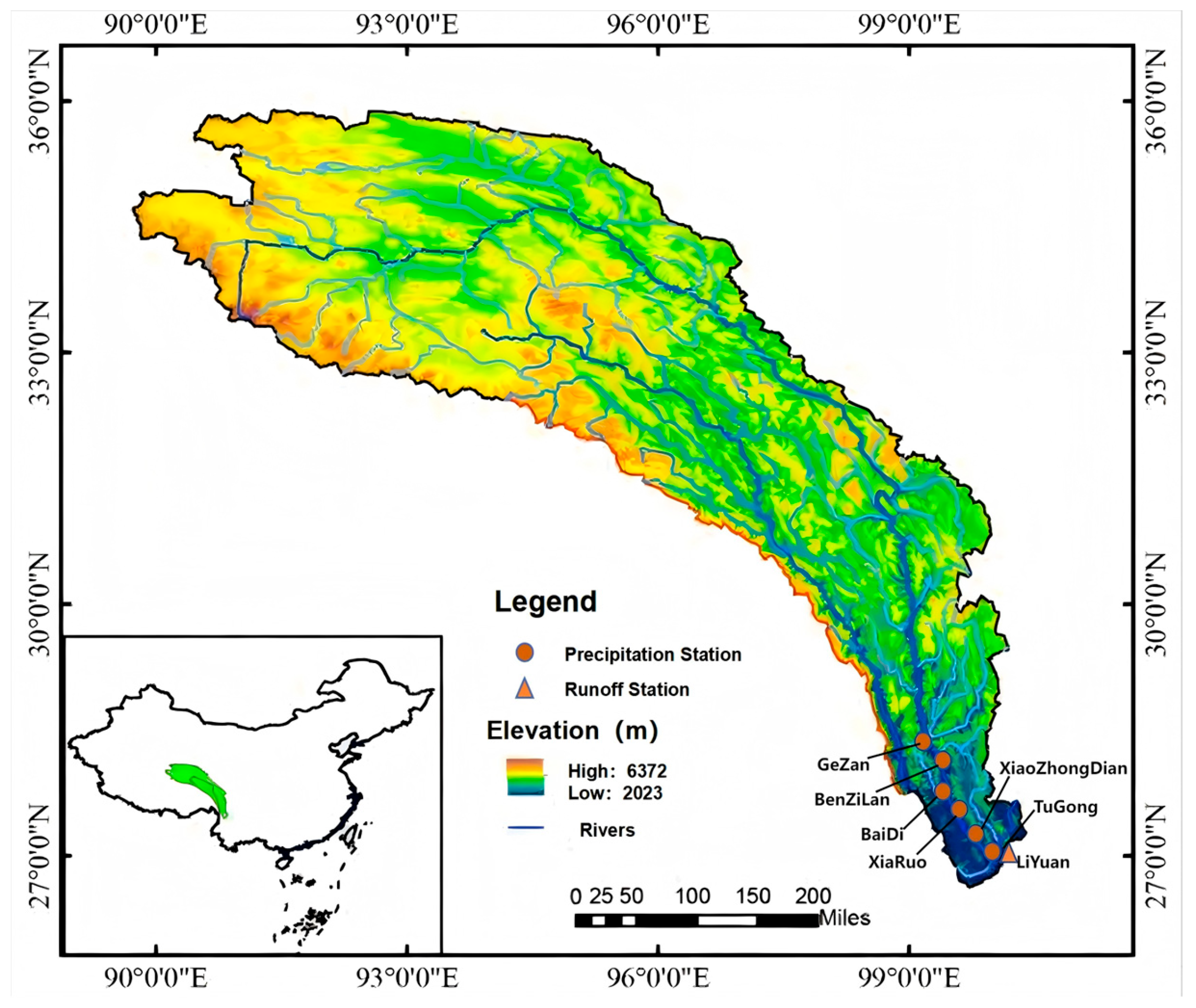
Figure 1. Research area map.
Water 17 02775 g001
Figure 2. Informer structure diagram.
Water 17 02775 g002
Figure 3. GRU structure diagram.
Water 17 02775 g003
Figure 4. Informer-GRU model architecture diagram.
Water 17 02775 g004
Figure 5. Predictive Flowchart.
Water 17 02775 g005
Figure 7. CEEMDAN decomposition result diagram.
Water 17 02775 g007
Figure 8. Comparison of runoff prediction of different models.
Water 17 02775 g008
Figure 9. Scatter plot of runoff prediction for different models.
Water 17 02775 g009
Figure 10. Comparative chart of runoff prediction in ablation test.
Water 17 02775 g010
Figure 11. Scatter plot of runoff prediction in ablation test.
Water 17 02775 g011
Figure 12. SHapley Additive exPlanations analytic result.
Water 17 02775 g012
Table 1. GTO optimization parameter comparison.
Optimization CategoryParameter TypeBefore OptimizationAfter Optimization
Dataset Parameterswindow size2426
Label length1213
Forecast step11
Model ArchitectureGRU hidden layers [110, 353, 499, 223][502, 303, 184, 393, 458, 169]
Transformer model dimension185350
Number of attention heads1112
Dropout rate0.06150.0735
Encoder layers23
Decoder layers21
Training HyperparametersLearning rate0.0000630.000095
Batch size4339
Maximum epochs3833
Multi-objective Loss WeightsMSE ( λ 1 )0.33990.3418
MAE ( λ 2 )0.24130.3624
Huber ( λ 3 )0.28800.2089
NSE ( λ 4 )0.14170.2404
Correlation ( λ 5 )0.11170.1475
Table 2. Model evaluation index results.
IndexValidation SetTest Set
R20.9564120.946936
NSE0.9564120.946936
KGE0.8253080.958182
RMSE268.26271.51
MAE181.49186.78
Table 3. Performance index comparison of different models in Liyuan Basin.
ModelR2NSERMSEMAEKGE
LSTM0.8828000.882800492.98322.470.838660
GRU0.8733010.873301419.54266.010.735504
Transformer0.8450000.845000383.46255.980.802750
Informer0.8550000.855000385.49246.830.812250
CNN-LSTM0.8377340.837734474.79308.230.727351
My Model0.9469360.946936271.51186.780.958182
Table 4. Comparison of performance indexes of ablation experiment.
ModelR2NSEMAEKGER2 Improvement
Informer (Baseline)0.7188690.718869422.570.7724140
+GRU0.8080960.808096371.680.82154212.41%
+STL0.8766470.876647263.400.8316778.48%
+CEEMDAN0.9106950.910695243.940.9308063.88%
+GTO0.9229860.922986206.680.9218281.34%
+Multi-Loss (MyModel)0.9469360.946936186.780.9581822.59%
Disclaimer/Publisher’s Note: The statements, opinions and data contained in all publications are solely those of the individual author(s) and contributor(s) and not of MDPI and/or the editor(s). MDPI and/or the editor(s) disclaim responsibility for any injury to people or property resulting from any ideas, methods, instructions or products referred to in the content.