Article

Evaluating Infiltration Methods for the Assessment of Flooding in Urban Areas

by
Paola Bianucci
1,2,
Javier Fernández-Fidalgo
1,2,
Kay Khaing Kyaw
3,
Enrique Soriano
1 and
Luis Mediero
1,2,*
1
Department of Civil Engineering: Hydraulics, Energy and Environment, Universidad Politécnica de Madrid, Calle del Profesor Aranguren 3, 28040 Madrid, Spain
2
Research Center for Intelligent and Sustainable Civil Infrastructure (CIVILis), Universidad Politécnica de Madrid, Calle Alfonso XII 3 y 5, 28014 Madrid, Spain
3
Department of Civil, Environmental, Chemical and Materials Engineering (DICAM), University of Bologna, 40126 Bologna, Italy
*
Author to whom correspondence should be addressed.
Water 2025, 17(18), 2773; https://doi.org/10.3390/w17182773
Submission received: 20 July 2025 / Revised: 29 August 2025 / Accepted: 2 September 2025 / Published: 19 September 2025
(This article belongs to the Special Issue Urban Flood Frequency Analysis and Risk Assessment, 2nd Edition)

Abstract

Urban flooding caused by short and high-intensity rainfall events presents increasing challenges for cities, threatening infrastructure, public safety and economic activity. Accurately representing infiltration processes in hydrodynamic models is critical, as oversimplifying infiltration can lead to significant errors in predicted flood extents and water depths. This study systematically compares two widely used infiltration models—Green-Ampt and Curve Number—implemented within two leading 2D hydraulic models, HEC-RAS and IBER, to assess their influence on urban flood predictions. Simulations were conducted for 26 rainfall events, including both observed and synthetic hyetographs, across two urban neighbourhoods in Pamplona metropolitan area, Spain. Model performance was evaluated using root mean square error, mean absolute error and confusion matrix-derived metrics such as precision, accuracy, specificity, sensitivity and negative predictive value. Results indicate that the choice of infiltration method significantly affects both water depths and inundation extents: while Green-Ampt yields more conservative water depth estimates, Curve Number tends to underestimate flood extents. The comparison between the two hydraulic models has shown that IBER simulates broader flood extents and lower water depth errors compared to HEC-RAS. The findings highlight the importance of selecting appropriate infiltration methods and hydraulic models for reliable urban flood risk assessment, as well as providing guidance for model selection in urban inundation studies.

1. Introduction

Urban flooding driven by short and high-intensity rainfall events poses growing challenges for cities worldwide. In addition, it will amplify risks to infrastructure, public safety and economic activity in the future. While stormwater drainage systems and surface topography often dominate pluvial flood assessment, infiltration critically controls the volume and timing of runoff, especially during short-duration and high-intensity storms. Either neglecting or oversimplifying infiltration processes in urban models can lead to substantial errors in predicted flood extents and water depths, as surface runoff may be overestimated when subsurface losses are ignored [1].
Infiltration plays a relevant role in rainfall–runoff processes. There are several methods available for assessing infiltration amounts. They can be grouped into three main categories regarding their formulation philosophy: physically based, semi-empirical and empirical methods. Physically based methods are based on the Darcy and mass conservation laws. The complexity of their formulations varies regarding the specific processes (fluxes relationships and dynamics) considered, initial and boundary conditions defined and dimensionality, among other factors. Some examples of physically based methods are the original Green and Ampt version (GA) [2], Philips (P) [3], Mein and Larson [4], Smith [5] and Smith and Parlange [6] models.
Semi-empirical methods are developed based on some simplifications of the continuity equation and the relation between infiltration rate and cumulative infiltration. In this category, models such as Horton (H) [7], Holtan [8], Overton [9], Singh and Yu [10] and Grigorjev and Iritz [11] can be found.
Finally, empirical methods are formulated by fitting mathematical models to datasets which were obtained from field and/or laboratory experiments. They usually depend on either one or a few parameters that need to be defined. Their applicability range usually depends on the conditions of the experiments that provided the datasets. Some examples of these methods are the Curve Number (CN) method proposed by the US-SCS [12], Kostiakov (K) [13] and its variations Modified Kostiakov (MK) [14] and Revised Modified Kostiakov (RMK), Huggins and Monke [15], and Collis-George [16].
In addition to the aforementioned formulations, hydrological practice has also widely adopted conceptual loss models that are not directly derived from soil physics but rather from simplified abstractions of rainfall–runoff processes [17]. These approaches conceptualize infiltration and other abstractions as lumped losses, thereby providing practical tools for large-scale or real-time applications where detailed parameterization is not feasible. The Initial Loss–Continuing Loss (IL–CL) and the Initial Loss–Proportional Loss (IL–PL) models allow straightforward implementation in event-based flood simulations and are particularly standard in regions such as Australia [18]. The IL represents the canopy and surface detention and infiltration before the runoff starts. It is related to the antecedent moisture condition. CL and PL represent the infiltration after the start of runoff. The first method depends on an infiltration rate, and the second one considers a fraction of the corresponding rainfall [19,20]. Similarly, related models such as the Runoff Coefficient approach are also applied in urban hydrology to directly relate rainfall to runoff volumes. Although such methods do not explicitly represent soil processes, their simplicity and ability to simulate the basin response make them a valuable tool for engineering design and flood assessment [20].
Some of the most widespread infiltration models include GA, H, K and P. Most previous studies are focused on analyzing areas with non-urban land uses and basins where urban coverage represents a small percentage. In [21], the authors assessed the factors affecting the infiltration rate in a river basin in Nepal by applying the HEC-HMS model considering the GA infiltration equation. The model outputs were compared with field measures. The authors concluded that the most relevant factor corresponds to soil coverage (or soil uses), having a higher impact than soil type or slope. An exponential relationship between rainfall intensity and infiltration rate was also noted.
Some recent studies proposed modified versions of commonly used models, improving their performance or adapting them to given conditions. In [22], the authors compared GA and K methods in small basins located in Equatorial climate regions. They validated the results of the models using field measurements. They concluded that GA provides better performance. They proposed a modification of the Kostiakov method oriented to improve it. Such a change in the formulation allows incorporating soil characteristics. In addition, in [23], a variation of the Horton method was proposed to adapt it to intermittent rainfall.
Other studies compared several infiltration models applied to cultivated and/or irrigated soils. In [24], the authors compared three infiltration methods (K, P and H) with field measurements for experimental agricultural and horticultural lands. Their findings showed the better performance of the P method. Other research efforts that compared several methods applied to agricultural lands are (H, P, K, MK, RMK and Novels) [25] and (GA, P, H, SCS, K, MK, RMK and Swartzendruber) [26]. Both studies observed that RMK and MK provided better performance than the other methods. In [27], Mishra and co-authors compared 14 models applied to 240 sites with available observed data. They used the Nash–Sutcliffe model efficiency coefficient (NSE) to measure the model performance, concluding that Singh-Yu, Holtan and H provided better results. They also found that all models present poor performances for sandy soils.
Recently, some researchers have combined machine learning techniques (ML) with hydrological models to improve their ability to represent infiltration processes for sites with low data availability. In this sense, in [28], the authors evaluated the response of P, H and K methods, comparing the results with their combination with ML methods, including an artificial neural network (ANN) and the missForest algorithm (MF). They used measured data of infiltration rates, cumulative infiltration, soil textures and moisture content. They concluded that H provides better results for sites with heterogeneous characteristics (soil type and coverage). They found that, in general, the hybrid model combining P and ML improved the infiltration estimates compared to traditional methods.
Despite extensive benchmarking of these methods in agricultural and watershed settings, their performance in urban zones remains less explored because of the inherent complexities and heterogeneity of such areas. Heterogeneous soil properties lead to spatial variability in infiltration rates, complicating parameterization and requiring extensive field data for calibration [29]. In addition, limited availability of high-resolution spatial data on soil characteristics and impervious surface distribution hampers model input preparation and increases uncertainty in urban areas [30]. Sparse field measurements and variability across urban sites lead to large uncertainties in model predictions, complicating validation and reducing confidence in simulated runoff and flood extents [29]. Regarding topography, irregular urban surfaces with buildings, roads and drainage networks also complicate the representation of flow paths and wetting-front dynamics in infiltration models [31]. Some studies have analyzed the effect of a set of factors on the accuracy of flood inventory maps [32,33,34]. They found that some of the most relevant factors in urban areas correspond to rainfall elevation and, in particular, the slope of the terrain. Their findings highlight the importance of a careful definition of model geometry. These studies also underscored the impact of land use and density of drainage systems on flood vulnerability in urban areas.
In [35], the impact of infiltration rate on runoff generation was studied. The authors modeled the infiltration through GA and H, comparing the results with measured data. They concluded that model responses deeply depend on the site characteristics and present a significant uncertainty, particularly for sandy soils. Other studies developed considering urban areas have focused on evaluating the impact of some elements on stormwater drainage. In [36], the interactions of different urban spaces and coverages were evaluated to improve stormwater runoff management. The infiltration rate was assessed using H contrasted with observed data. They concluded that it is effective to provide sparse green areas to manage urban stormwater runoff. Sage and co-authors [37] proposed a conceptual model combining infiltration (GA) and flow redistribution (similar to the method included in the EPA-SWMM). They compared the performance of the conceptual model with traditional Richards and GA models, finding that the conceptual model improves the precision of infiltration rate estimation, particularly when assessing rain garden performance. Combining traditional infiltration models with simulation models (allowing flow redistribution) and with ML constitutes a promising set of techniques for properly assessing rainfall–runoff transformation in urban areas and the impact of infiltration rates.
Spatial clustering of impervious areas creates highly variable local infiltration responses during storm events, requiring models to resolve fine-scale land-cover patterns for reliable predictions [38]. However, few investigations have systematically evaluated how the choice of the infiltration method interacts with two-dimensional (2D) hydraulic simulation tools and influences predicted inundation patterns in urban environments.
This paper addresses such a gap by comparing two widespread infiltration equations with two leading 2D hydraulic models to evaluate urban pluvial floods driven solely by stormwater runoff. We apply each model combination to two urban case studies under a set of design storm hyetographs (synthetic and observed). Then, we quantify differences in predicted flood extents and water depths using raster-based image analysis and error metrics. By isolating infiltration effects from riverine and tidal influences, our results elucidate how infiltration parameterization shapes urban flood risk assessments.
The paper is organized as follows: Section 2 explains the methodological framework and describes the case studies; Section 3 presents and discusses the obtained results. Finally, Section 4 summarizes the main findings and provides recommendations.

2. Materials and Methods

2.1. Case Study

The study focuses on two urban neighborhoods in the Pamplona metropolitan area (Spain): Barañáin and Zizur Mayor. Both areas exhibit mixed impervious and pervious surfaces and are representative of mid-size Mediterranean cities. Their geographic location is depicted in Figure 1.
To characterize the case study sites, the geographical information provided by the National Geographic Institute (Instituto Geográfico Nacional, IGN, in Spanish) was employed. In particular, the following shape and raster layers downloaded from the official website [39]:
  • Digital elevation (terrain and surface) models (DEMs).
  • Land cover (CORINE Land Cover project).
  • Soil cover.
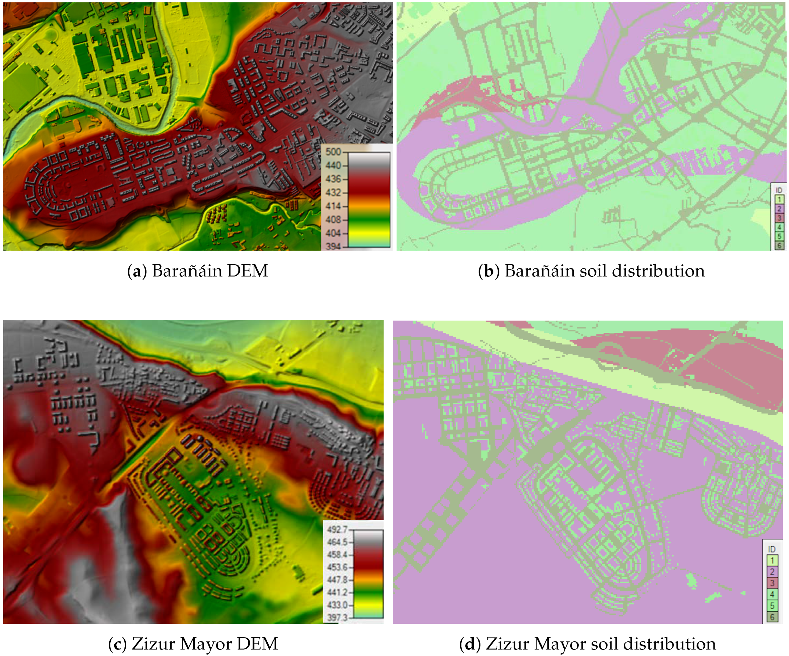
For both models, the meshes in the hydraulic models were defined based on the DEMs, depicted in Figure 2a,c. Based on the soil distribution, we assigned the GA and CN model parameters as shown in Figure 2b,d. Land-use and lithology layers were used to identify soil types in the Pamplona metropolitan area. More specifically, land-use maps provided by the IGN and the COoRdinantion of INformation of the Environment (CORINE) Land Cover (CLC 2018) project were used. Values of the GA an CN parameters for each soil type were obtained from the literature based on previous experience [40].
The hydraulic models for both sites were fed with several rainfall events to simulate the corresponding flooding. Four observed spatially distributed events were considered [41]:
  • 20 July 2010—6:30 p.m. to 7:20 p.m.
  • 20 July 2010—9:10 p.m. to 10:40 p.m.
  • 18 September 2019—6:30 a.m. to 7:20 a.m.
  • 18 September 2019—4:00 p.m. to 4:50 p.m.
For each event, quantitative precipitation estimation (QPE) fields were obtained with time steps of 10 min [41]. For example, Figure 3 shows the rainfall spatial distribution for 10 min time steps from 9:10 p.m. to 10:40 p.m. on 20 July 2010, corresponding to the Barañáin case study. Each of the grayscale raster maps in this figure shows the spatial distribution of the QPE for the corresponding 10 min interval (starting at the time indicated in a corner of each map). In addition, the corresponding point rainfall hyetographs were defined and evaluated for two of these episodes.
Furthermore, we used seven combinations of rainfall depth (P), from 20 mm to 60 mm, and duration (D), from 1 h to 3 h, associated with a set of return periods (Trs), between 2 and 200 years. Three intensity peak positions were considered for each P-D combination (centered, left-skewed and right-skewed). Thus, we assessed the response to 21 synthetic hyetographs, with 15-min time-step point rainfall, as depicted in Figure 4.
In total, for each site, we simulated 26 rainfall events considering two different infiltration methods (GA and CN) and applying two 2D hydraulic models (IBER and HEC-RAS). Therefore, 104 simulations were run for each site (Barañáin and Zizur).
For a clearer presentation of the case studies, Table 1 summarizes the data used to implement the hydraulic models and its main characteristics (source, resolution and specific application).
Analogously, Table 2 summarizes the settings of the hydraulic models implemented in this research. Explanation and justification for the selection of the applied models can be found in Section 2.2.

2.2. Methodological Framework

The proposed methodology involves two-dimensional (2D) hydrodynamic models fed with rainfall inputs. Infiltration is explicitly simulated as a component of the rainfall–runoff transformation process by implementing an infiltration method, among the ones available in each hydraulic model. The hydraulic models allow flow (runoff) redistribution, determining water depths and flooding extent derived for a given storm event.
Physically based 2D shallow-water models solve non-linear partial differential equations on fine meshes, requiring small time steps for numerical stability and leading to high CPU and memory use. Simplified or diffusive-wave approximations reduce run times but omit critical dynamics, such as inertial or viscous effects, compromising accuracy under complex urban flow regimes. Additionally, high-resolution digital terrain models (DTMs) with detailed building footprints and street geometry generate large datasets that increase preprocessing times and computing requirements, which may exceed conventional computation capabilities [31].
In this study, two widely spread and tested 2D hydraulic models were used: HEC–RAS [43] and IBER [44]. We apply two infiltration methods, GA [40] and CN [45], assessing the impact of using a given infiltration equation on the resulting flooding. We chose such infiltration methods because they are available in both hydraulic models and due to their extensive dissemination and level of implementation worldwide.
The hydraulic models were fed with a set of rainfall patterns: four spatially distributed observed precipitation events, two observed hyetographs (point rainfall) and 21 synthetic hyetographs, which were defined for seven combinations of rainfall depth and duration (associated with a set of return periods) and three rainfall intensity peak positions (centered, right-skewed and left-skewed).
The main results analyzed are both maximum water depths and flood extents, provided for each combination of hydraulic model, infiltration formulation and rainfall event. We evaluated the results in raster format through image analysis. First, we computed error indicators, such as MSE, RMSE and MAE, by comparing the water depth rasters corresponding to two model settings. Therefore, the following pair comparisons were implemented:
  • The two rasters related to a given hydraulic model and rainfall storm, but with infiltration computed with the two different methods.
  • The two rasters derived from the two hydraulic models fed with the same rainfall storm and applying the same infiltration method.
In order to quantify the effects of the infiltration and hydraulic models, we employ several metrics which provide systematic measures of error. The chosen metrics were the following: root mean square error (RMSE), mean absolute error (MAE), and metrics derived from confusion matrixes. These matrixes provides various measures based on the comparison of positive and negative values: true positives (TPs), false positives (FPs), true negatives (TNs) and false negatives (FNs). This set of metrics includes precision (PRE), accuracy (ACC), specificity (SPEC), sensitivity (SENS) and negative predictive values (NPVs), among others. In order to calculate the aforementioned metrics we used the definitions described in [46,47].
RMSE measures the square root of the mean of the squared errors, providing an estimate of the average magnitude of the error and penalizing larger errors more severely. In contrast, MAE calculates the mean of the absolute values of the errors, offering a direct measure that is less sensitive to outliers compared to RMSE. Both metrics allow for the interpretation of model accuracy in the original units of the variable of interest, facilitating comparison and interpretation of the results.
Additionally, for classification tasks, a set of metrics derived from the confusion matrix were used, such as PRE, ACC, SPEC, SENS and NPV [46,47]. While PRE indicates the proportion of TPs among all positive predictions, ACC reflects the proportion of correct predictions over the total number of evaluated cases. SPEC measures the model’s ability to correctly identify negative cases, and SENS (or recall) assesses the ability to correctly detect positive cases. NPV represents the proportion of TNs among all negative predictions. False positive rate (FPR or fall-out) is the proportion of actual negatives incorrectly classified as positive, while false negative rate (FNR or miss rate) indicates how often a model fails to detect actual positive cases. The combined use of these metrics provides a comprehensive view of model performance, allowing for the identification of strengths and weaknesses in detecting different types of events or classes, which is a fundamental aspect in critical applications such as water resource management.
We also analyze the effect of the rainfall patterns, particularly for the synthetic hyetographs with the same rainfall depth and duration but different intensity peak positions.
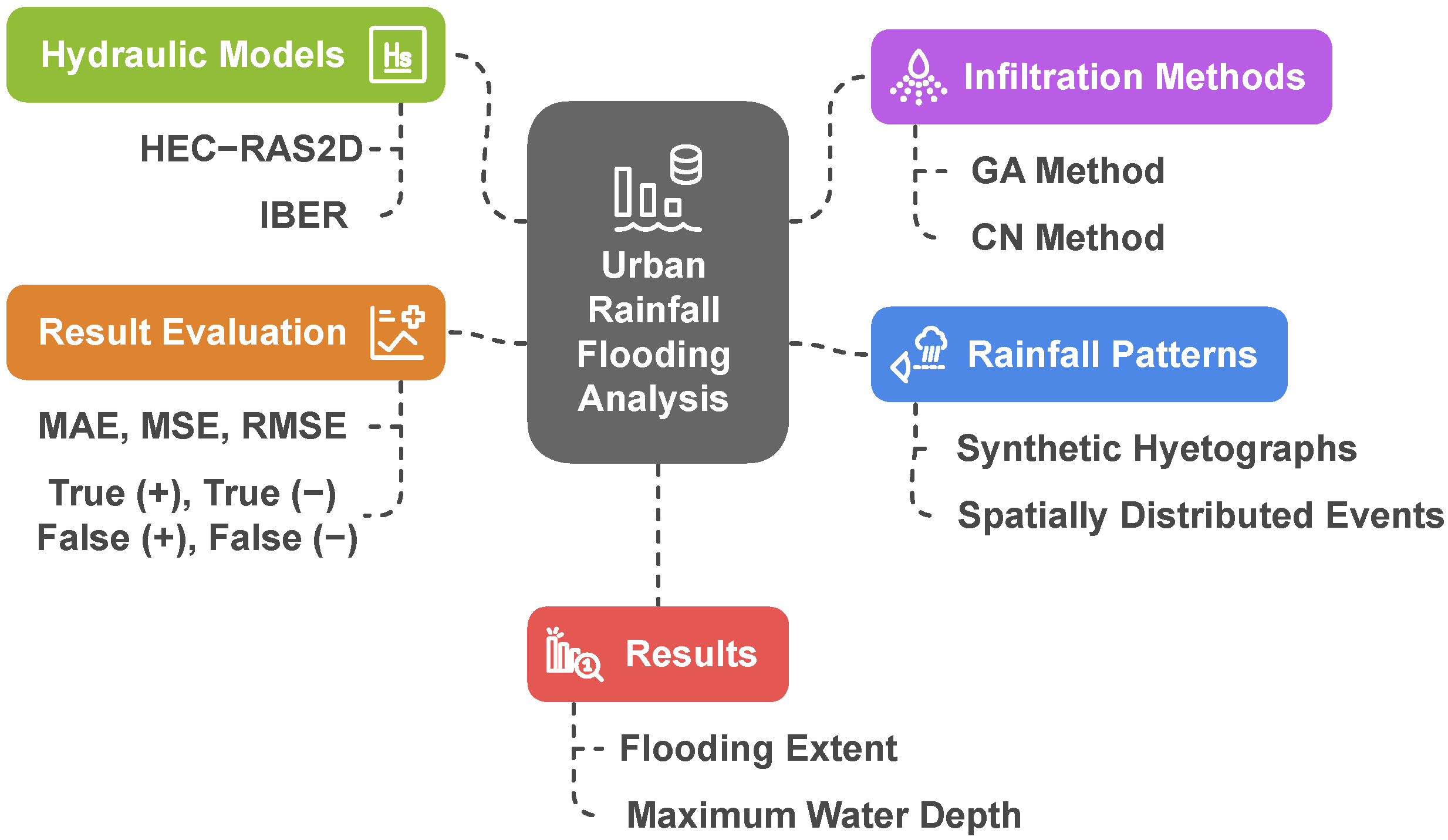
The methodological framework is synthesized in Figure 5.

3. Results

3.1. Simulation Results

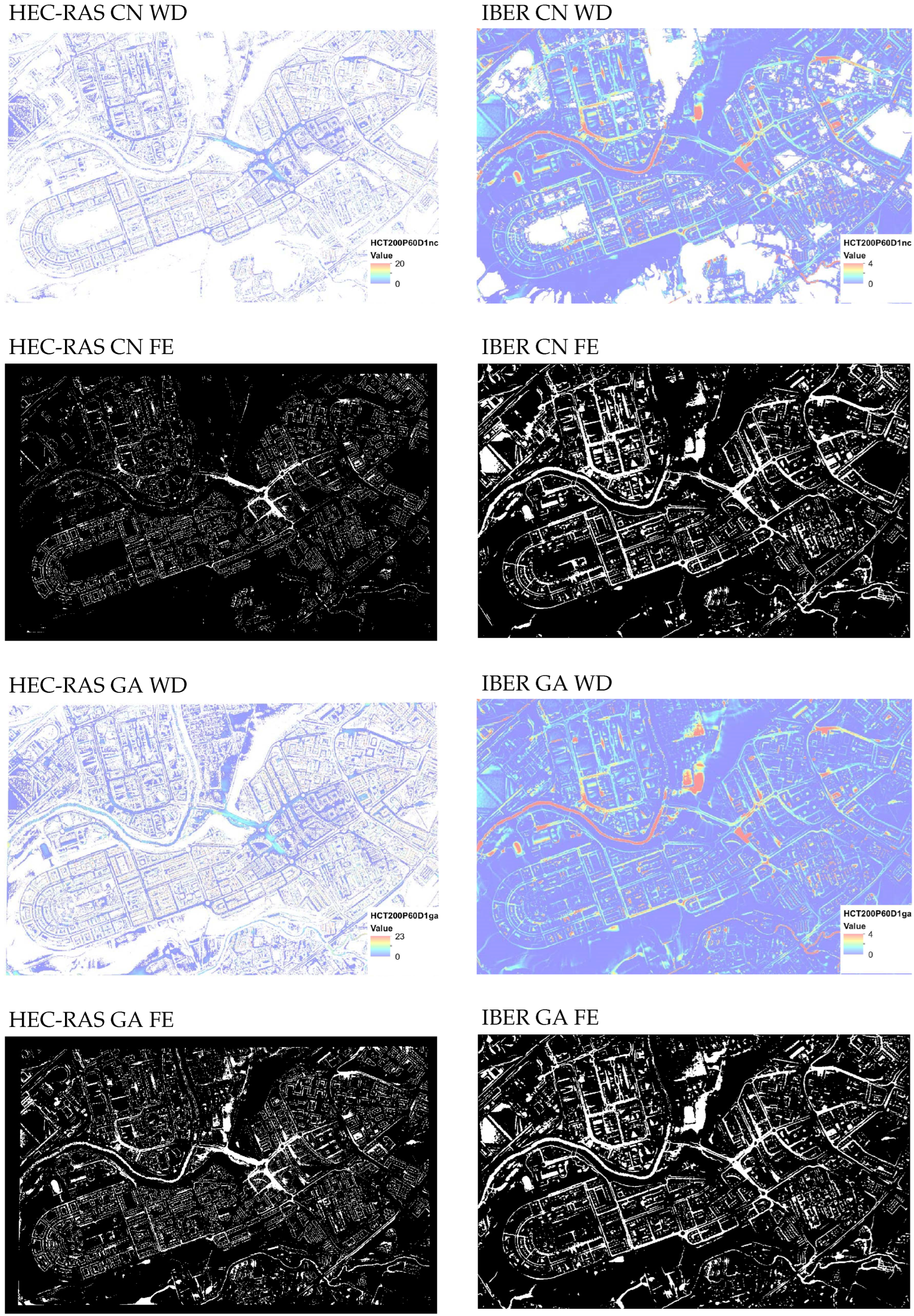
We simulated the set of 26 rainfall events for both sites, considering two infiltration methods and two hydraulic models, leading to a total of 208 simulations. For each simulation, we obtained the corresponding spatially distributed water depth layer. To keep a clear presentation, we show here the results for the Barañáin (Figure 6) and Zizur Mayor (Figure 7) case studies, corresponding to the synthetic hyetograph with P = 60 mm, D = 1 h and a centered intensity peak (HCP60D1).
We observed that the HEC-RAS model tends to assign wrong water levels in some cells. For example, it tends to identify wet cells on top of roofs. In other cases, such errors may be related to the terrain height defined in the hydraulic model mesh generated from the DEM. These errors caused some cells to have extremely high or low water depths. Consequently, we proceeded to identify and remove the cells with such wrong water levels.
Therefore, in this analysis of 208 simulations with the IBER and HEC-RAS hydraulic models, anomalies in the HEC-RAS results that could distort comparisons were identified. Specifically, certain water depths in HEC-RAS were unrealistic outliers. For example, in a simulation for a 20 mm rainfall event (with a 1-h duration and 2-year return period), the maximum water depth reached 17 m in given cells, which is highly unrealistic. A comparison of water depth distributions (Figure 8) shows that while most of the IBER predictions are close to 0 m, with few extreme values, the HEC-RAS results are also clustered close to 0 m but include a long right tail extending up to 17 m. This indicates that HEC-RAS tends to predict larger and more extreme water depths, revealing outliers that must be addressed for an accurate comparison with IBER results.
In addition, we also identified similar anomalies in other HEC-RAS simulation results, where water depths exceeded the expected values for the rainfall storms considered as input. Therefore, we flagged outliers with water depths greater than 5 m, which was considered as a reasonable threshold for exclusion. This revealed 48 outliers in Zizur Mayor and 378 in Barañáin (Figure 9), all located at the same geographic points across simulations. Such outliers were usually found on buildings, likely due to either HEC-RAS misinterpreting building heights as water depths or from errors in terrain data handling. All identified outliers were removed from the HEC-RAS results to ensure accurate comparisons with IBER.
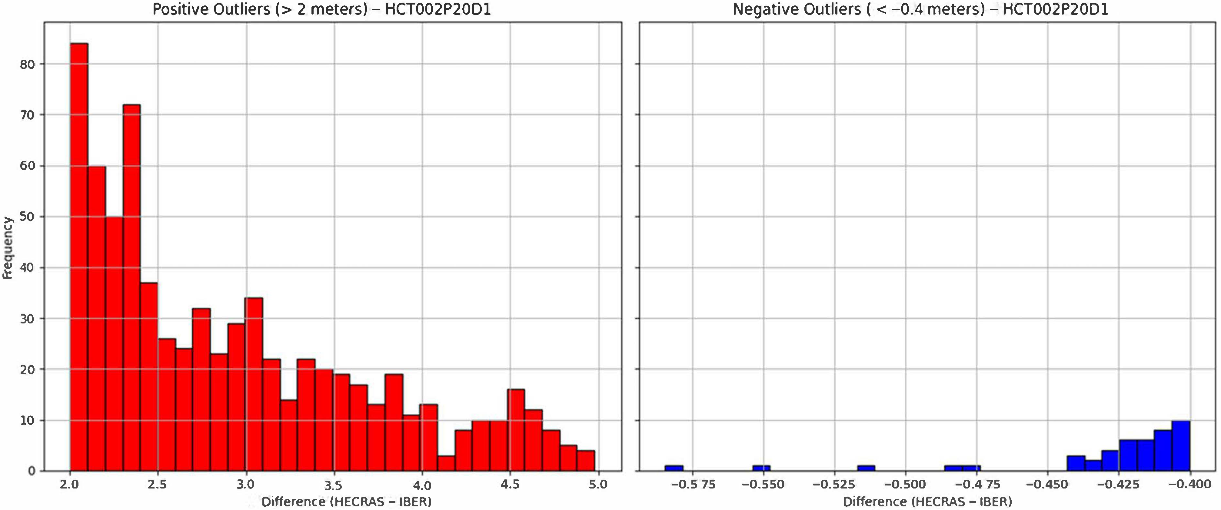
After removing extreme water depth outliers, we analyzed positive and negative outliers by examining water depth differences between HEC-RAS and IBER. The left panel of Figure 10 shows the frequency of positive differences (HEC-RAS—IBER > 2 m), where HEC-RAS predicts significantly higher water depths, with some differences exceeding 5 m. The right panel of Figure 10 shows the frequency of negative differences (HEC-RAS—IBER < −0.4 m), where HEC-RAS predicts slightly lower depths than IBER. While positive outliers indicate frequent overprediction by HEC-RAS, negative outliers are less frequent and relatively minor. To ensure accurate comparisons, both types of outliers were removed from the HEC-RAS simulations. The updated water depth distribution (Figure 11) demonstrates significant improvement compared to the initial distribution (Figure 8).

3.2. Model Comparisons and Performance Assessment

The maximum water depth and flood extent raster output layers were compared by applying the metrics mentioned in Section 2. The authors applied a pair comparison to assess the effect of the infiltration methods (for the same event and hydraulic model) and the influence of the hydraulic model (for the same event and infiltration method).
For water depth comparison, the authors considered RMSE and MAE metrics, while for flood extent analysis, the metrics related to the confusion matrixes were applied.

3.2.1. Effect of Infiltration Method

Table 3, Table 4, Table 5 and Table 6 synthesize the values obtained for the metrics included in Section 2. For the comparison regarding the infiltration models, GA was considered as the ground truth value.
Across 208 simulations (26 storm events × 2 infiltration methods × 2 hydraulic models × 2 study sites), flood water depths and inundation extents varied systematically with both the infiltration methods and hydraulic models. The GA method yields consistently higher water depths than the CN method, with mean RMSE values of 0.15 m versus 0.12 m with HEC-RAS and 0.18 m vs. 0.14 m with IBER. RMSE increases with total rainfall depth, reaching 0.25 m for the 60 mm events.
The CN method tends to underestimate flood extents by up to 10% compared with the GA method, especially across pervious-to-impervious transition zones. When comparing hydraulic models, IBER simulates inundation extents approximately 5% larger than HEC-RAS under identical conditions, exhibiting lower water depth errors (mean MAE values of 0.08 m vs. 0.10 m). Confusion-matrix metrics reveal SPEC above 90% in all scenarios. However, SENS falls below 75% for right-skewed intensity peak synthetic storms. This indicates that, under these conditions, the models are less capable of detecting all the areas that actually become flooded, especially those that are inundated towards the end of the rainfall event.
For the HEC-RAS model, higher P values are related to high error metrics (RMSE and MAE) and small NPV, SPEC and ACC values. ACC values remained stable across all analyzed events. However, SENS values increased when P rose from 40 mm to 60 mm, but their peak was obtained at 20 mm, exhibiting high variability depending on storm duration. Other metrics showed minimal dependence on storm duration and hyetograph peak position.
For the IBER model, errors increased with intermediate P amounts (40–60 mm) and were notable with a low P of 20 mm due to limited runoff generation for such precipitation amounts. NPV values were consistent across P values, with minor variations tied to storm duration. ACC and SENS followed similar trends: SENS values decreased for right-skewed precipitation peaks and increased for left-skewed ones. While SPEC remained stable (93–95%) across scenarios, PREC improved with higher P values and right-skewed storms.

3.2.2. Effect of Hydraulic Model

The comparison of the RMSE and MAE values between the IBER and HEC-RAS hydraulic models using the CN and GA infiltration methods reveals similar performance differences across the events, as depicted in Figure 12. In terms of RMSE values, the CN method consistently showed slightly lower error values compared with the GA method, with the highest RMSE values found in the 2010 storm event. Similarly, the analysis with MAE showed the same trend. The GA method exhibited higher absolute errors than the CN method, again with the 2010 storm event showing a similar MAE value for both infiltration methods. These results suggest that the GA method produces higher water depths than the CN method.
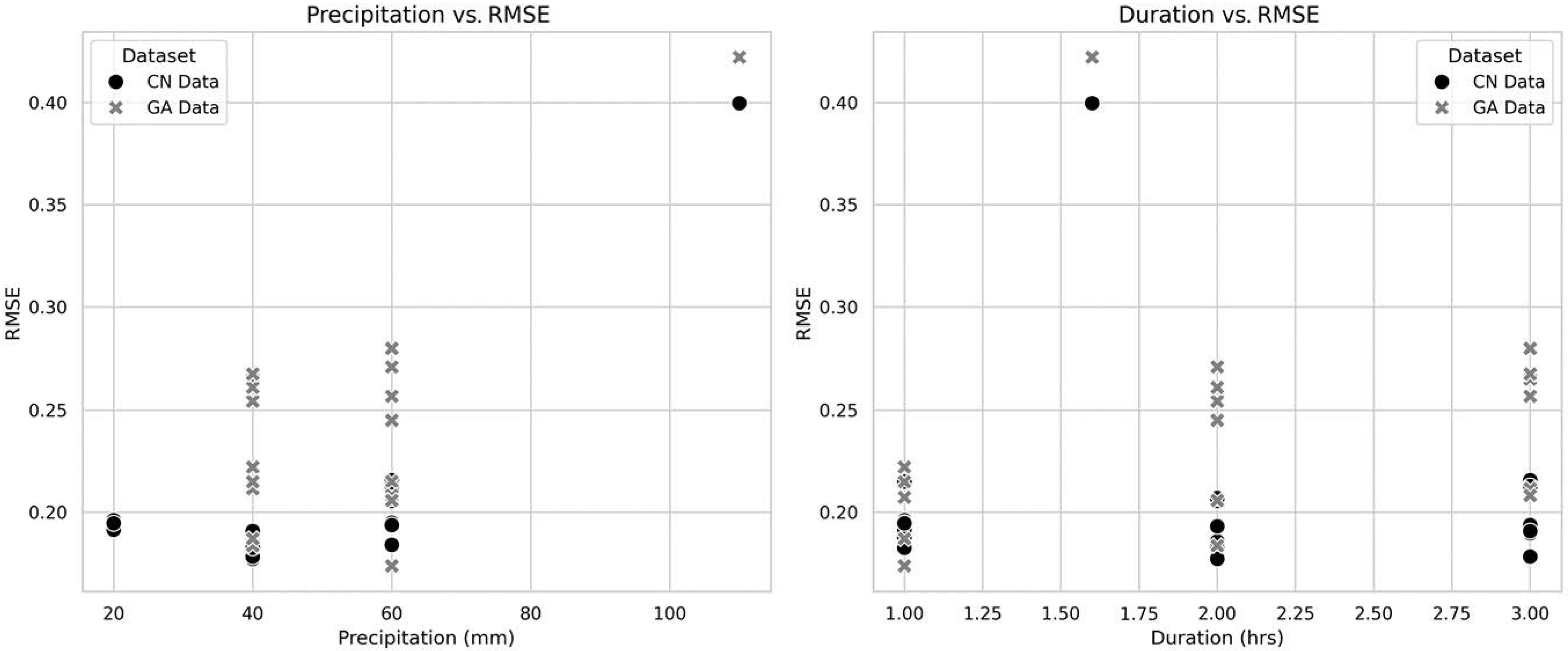
Authors also checked the relationship between RMSE values and storm precipitation and duration, shown in Figure 13. In terms of precipitation amount in each event, RMSE values generally increase as precipitation also increases, with both infiltration methods showing higher error values for events with greater precipitation, such as the 2010 storm event. Similarly, for event duration, RMSE values appear to marginally increase with longer durations, though the trend is less pronounced. The GA method exhibits slightly higher RMSE values compared with the CN method across both precipitation and duration values.
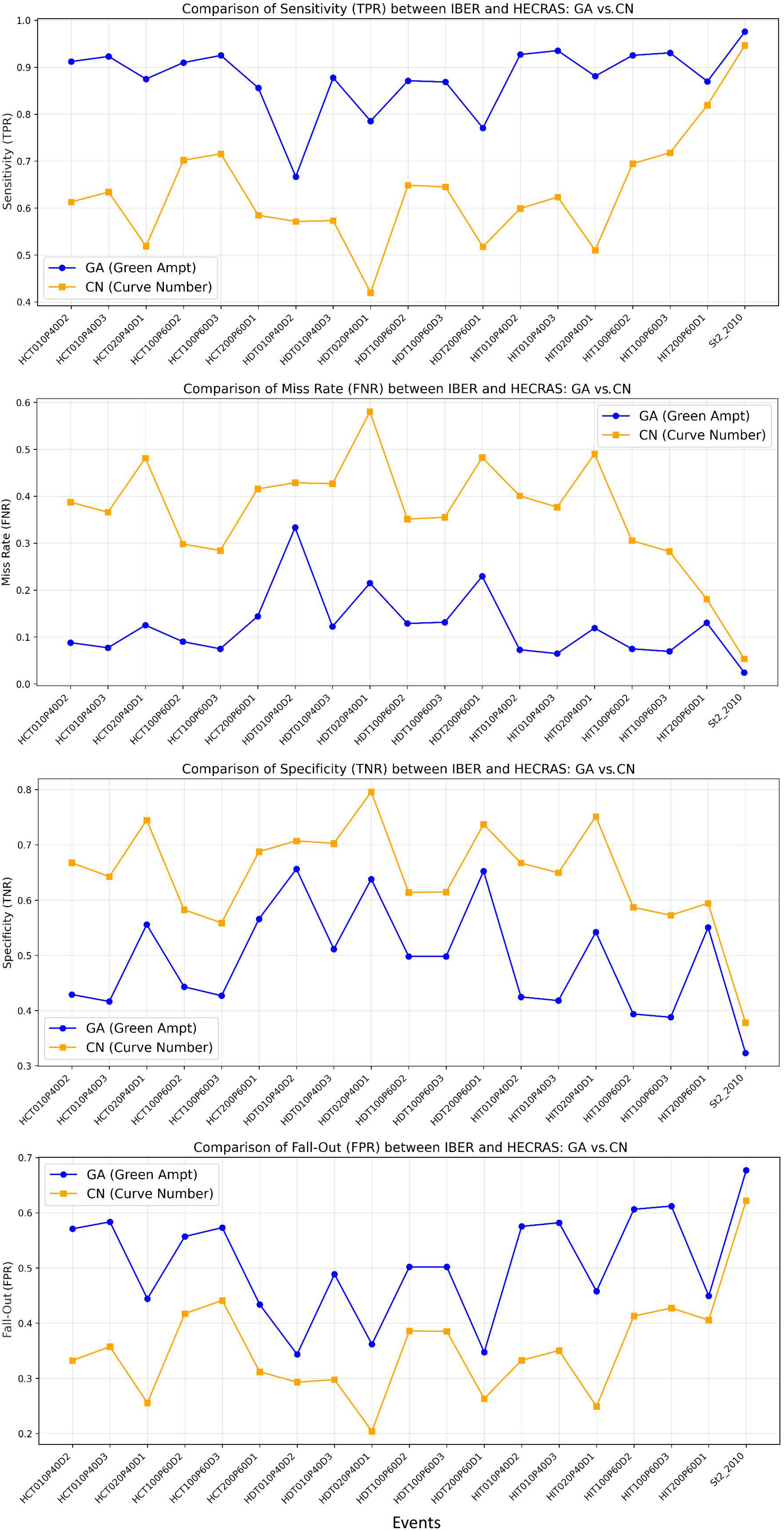
In addition, authors compared the flooded extent area using performance matrices between the IBER and HEC-RAS models using the GA and CN infiltration methods (Figure 14). The GA method exhibits consistently higher SENS values than the CN method, indicating its better ability to detect the occurrence of flooded cells. However, the CN method generally demonstrates higher SPEC, reflecting its stronger performance in identifying non-flooded areas. While the miss rate is lower for the GA method, aligning with its higher SENS, the CN method shows slightly lower fall-out, indicating fewer false alarms. These variations highlight distinct trade-offs between the two methods in predicting flooded area extents.
The relationship between SENS (sensitivity or true positive rate, TPR) and storm precipitation and duration shows clear trends for both CN and GA methods, as seen in Figure 15. SENS increases with higher storm precipitation, indicating better detection of flooded pixels under intense rainfall conditions. The GA method consistently exhibits higher SENS than the CN method across all event precipitation amounts. Similarly, SENS improves with longer storm durations, with the GA method outperforming the CN method. These results highlight the superior performance of the GA method in detecting flooded cells under varying precipitation intensities and durations.
The flooded area extent comparisons were conducted by analyzing the metrics within the HEC-RAS models and the IBER models separately, focusing on their performance under different infiltration methods, shown in Figure 16. The comparison of flooded area extent simulations within the two models, based on the GA and CN infiltration methods, reveals distinct trends. For HEC-RAS, while the GA method demonstrates consistently higher sensitivity, indicating better detection of flooded areas, the CN method shows improved specificity values, reflecting stronger performance in identifying non-flooded areas. Within the IBER models, both infiltration methods (GA and CN) exhibit strong performance in terms of specificity and fall out, indicating their ability to accurately identify non-flooded areas while maintaining fewer alarms. The GA method in IBER models also achieves higher sensitivity and lower miss rates compared with the CN method.
According to the comparisons of RMSE and MAE values between the IBER and HEC-RAS hydraulic models, the observed trend of slightly lower RMSE and MAE values for the CN method compared with the GA method suggests that both methods perform similarly in representing maximum water depths in this study. The differences in RMSE values between the two methods are minimal, of approximately 5 cm, which can be considered as not significant. This indicates that both methods provide comparable accuracy for the analyzed storm events. The empirical nature of the CN method may simplify the characterization of the infiltration process, aligning well with the specific characteristics of the storm events. Meanwhile, the GA method, which is more process-based, introduces additional complexity and parameter sensitivity, which could explain the slightly higher errors. Water depths simulated by the CN method are slightly lower than the GA method. Therefore, they may correspond to smaller runoff amounts. Ref. [48] agrees with our findings that while both the GA and CN method have high correlation coefficient values, the CN method provides smaller runoff estimates compared with the GA method for modeling rainfall–runoff processes in ungauged watersheds.
The analysis of the relationship between RMSE values and storm precipitation and duration indicates that RMSE values depend on both variables. Higher storm precipitation amounts tend to result in larger errors, likely due to the increased complexity of runoff and infiltration processes. These findings are consistent with those of [49], who observed that the RMSE of water depths increased consistently with higher precipitation levels across return periods in their study on urban stormwater modeling. Similarly, the slight rise in RMSE with longer durations may reflect the accumulated challenges of modeling prolonged events which involve dynamic changes in soil saturation and flow conditions over time.
Results from the flooded area extent comparisons using performance matrices between the HEC-RAS and IBER models suggest that the GA method is more effective in detecting flooded cells, as indicated by its higher SENS and lower miss rate values. To the best of our knowledge, no existing studies have explicitly demonstrated that the GA method can detect more flooded areas than the CN method. However, ref. [50] found that the GA model outperformed the CN method in estimating both runoff volume and peak discharge across most watersheds in their study. We believe that their findings provide additional support for our conclusion. This makes GA a better choice in applications where capturing all flooded areas is critical. However, the CN method’s higher SPEC and lower fall-out indicate a stronger ability to avoid FPs, which may be beneficial in studies where overprediction of flooded areas can have significant consequences.
The relationship between SENS (TPR) and event precipitation and duration reveal that sensitivity is significantly influenced by both precipitation intensity and event duration. Higher precipitation levels likely amplify the distinctiveness of flooded pixel signals, particularly for the GA method. The increased SENS values observed with longer durations may indicate improved model performance as runoff dynamics become more evident over time. The GA method, with its consistently higher SENS values, shows greater reliability in detecting flooded areas, making it an ideal choice for applications that require precise runoff identification. This aligns with the findings of [51], who, despite focusing on highly agricultural areas rather than urban flooding, found that the GA model outperformed the CN model in accurately predicting large streamflow events. The GA model’s ability to accurately handle large hydrological events, as highlighted in their study, supports its effectiveness in identifying flooded areas in urban environments, where extreme runoff events are a key concern. Together, these findings suggest the versatility of the GA method across different hydrological applications.
An analysis of the behavior of the HEC-RAS and IBER hydraulic models individually has been conducted, examining the trends within each model by comparing their results under different conditions. The performance trends observed within both the HEC-RAS and IBER models, particularly in terms of the infiltration methods, highlight that the GA method is generally more effective in detecting flooded areas, as evidenced by its higher SENS values and lower miss rates. However, the CN method shows higher SPEC and lower fall-out values within both models, making it suitable in scenarios where minimizing false alarms is essential. Notably, the IBER models, regardless of the infiltration method, perform exceptionally well in terms of SPEC and fall-out values, suggesting their reliability in identifying non-flooded areas. Therefore, IBER models with the GA method effectively balance the trade-off between detecting flooded areas and minimizing false predictions, making them the most reliable choice across all performance matrices. The trends discussed here are specific to comparisons made within HEC-RAS models and within IBER models based on their respective infiltration methods (GA and CN). These results should not be interpreted as a direct comparison between the HEC-RAS and IBER models. The comparison between the HEC-RAS and IBER models when using the same infiltration method was already discussed in the above paragraphs.
The diffusion wave approximation simplifies the modeling process by neglecting acceleration effects and assuming equilibrium between gravitational and resistance forces, making it particularly effective for simulating urban floods, where interactions between water flow and urban infrastructure are highly complex [52]. Despite the challenges posed by intricate flow dynamics and irregular geometries, studies have shown that simplified models can produce comparable results to more complex models in terms of flooding extents, depths and exchanged volumes, while offering the advantage of reduced computational costs [53]. However, significant differences were observed in specific aspects of flow behavior, such as in the receding limb of the flood hydrograph, where the Gravity Wave Model (GWM) and Shallow Water Equations (SWE) provided smoother transitions compared to the Parallel Diffusion Wave (PDWAVE) model, which exhibited higher hydraulic heads and discharges at most manholes. These findings underscore the potential of simplified models for efficient flood modeling while highlighting the importance of model selection depending on the specific requirements of a study [53].

3.3. Considerations Regarding Study Limitations

Although an extensive analysis was performed, including a large number of simulations covering a reasonable variety of scenarios and settings, there are some aspects that may limit the applicability of the study’s conclusions.
The heterogeneity of soil coverage and the distribution of impervious surfaces in urban areas increase the complexity and uncertainty when trying to achieve a rigorous definition of model parameters. The methods in this study were applied to a particular area with specific characteristics. Extending the study to urban areas with different characteristics would help expand the conclusions and their applicability. However, the chosen sites present pervious (green urban facilities) and impervious (buildings and streets) areas which are representative of mid-size European cities.
The sensitivity of infiltration models, such as GA, to saturated hydraulic conductivity requires careful the choosing and calibration of their parameters. However, the lack of accurate data for calibration makes this task difficult. A sensitivity analysis may provide insight regarding this aspect. Although we did not apply this kind of assessment, we used contrasted values for the model parameters, which may reduce their impact on the results when comparing the infiltration methods (for the same hydraulic model). For hydraulic model comparison (same infiltration method and parameter values), the influence of not calibrating them could be neglected. Further research could be developed for deepening the knowledge regarding the effect of parameters on model performance when applied to urban areas, both thorough sensitivity analysis and field experiments (adjusted to urban environment conditions).
Machine learning (ML) techniques can significantly improve the accuracy, spatial resolution, and adaptability of infiltration assessments in urban flood modeling. By learning complex, non-linear relationships from diverse datasets, ML models overcome many limitations of traditional, parameter-driven methods. Random forest models trained on soil texture, land use, impervious cover and limited field measurements can generate high-resolution maps of infiltration rates across urban watersheds, capturing the strong heterogeneity of urban soils and reducing overestimation of runoff [54]. Combining classical infiltration formulas with ML is a promising technique [28,54] for enhancing the accuracy of urban flooding assessment associated with rainfall episodes. These techniques enhance the precision, spatial granularity and adaptability of infiltration assessments in urban flood modeling by capturing non-linear patterns from different data sources. Recent research demonstrates that ANN models, when calibrated with minimal yet strategically selected inputs such as precipitation and upstream catchment flow, can simulate dynamic urban runoff with substantially higher correlation, efficiency and generalization performance compared to traditional hydrological models [55]. Moreover, where detailed hydrodynamic or hydraulic data are scarce, ML classifiers employing readily accessible geo-environmental variables have proven to be of high accuracy, confirming ML’s efficacy in flood hazard mapping and its suitability for early-warning and urban planning applications [56,57].
Incorporating information about drainage systems could be particularly relevant for accurate modeling of events related to low return periods that are consistent with the design of stormwater networks [32]. However, when evaluating events with medium to high return periods, the influence of the drainage system on the results decreases. Although the present study considers a set of events with differing rainfall magnitudes, it does not focus on assessing the actual flooding extents when rainstorms occur, but rather on comparing the performance of both infiltration and hydraulic models. Furthermore, the lack of information on the characteristics of the stormwater networks justifies their exclusion in this study.

4. Conclusions

An extensive analysis was conducted assessing the effect of two infiltration methods (Curve Number and Green-Ampt) and two 2D hydrodynamic models (IBER and HEC-RAS) on pluvial or rainfall-driven urban floods, performing a total of 208 simulations. Usual metrics were considered for comparison purposes, such as RMSE and MAE for water depth analysis and metrics derived from confusion matrixes for flood extent comparison.
First, we assessed the effect of the infiltration method considering the same hydraulic model, and, second, the influence of the hydrodynamic model when applying the same infiltration method.
To determine the suitability of both models for use, we analysed comparisons considering both IBER as the reference and HEC-RAS as the reference. When IBER is used as a reference, HEC-RAS demonstrates high sensitivity (averaging around 0.65 in most scenarios), indicating that it detects a significant proportion of the flooded areas identified by IBER. However, the fall-out (false positive rate) is relatively high in many scenarios (0.30–0.40), which shows that HEC-RAS tends to overpredict flooding compared to IBER. In contrast, when HEC-RAS is used as the reference, IBER demonstrates excellent specificity (averaging 0.85–0.95), which means that it performs well in identifying non-flooded areas compared to HEC-RAS. IBER also significantly reduces false alarms, as reflected in its low fall-out rates (0.01–0.15 in most cases). However, IBER has low sensitivity (averaging around 0.30), which means that it misses a substantial number of flooded areas detected by HEC-RAS. In general, HEC-RAS is better suited for scenarios where detecting flooded areas (high sensitivity) is critical, such as flood risk management or early warning systems. However, its tendency to overpredict flooding should be considered, as it may result in false alarms. However, IBER is more appropriate for applications where minimizing false positives is essential, such as urban planning or flood insurance assessments, where overprediction could lead to unnecessary costs.
The Curve Number method tends to underestimate flood extents by up to 10% relative to the Green-Ampt method, especially across pervious-to-impervious transition zones. When comparing hydraulic models, IBER simulates inundation extents approximately 5% larger than HEC-RAS under identical conditions, while exhibiting lower depth errors (mean MAE values of 0.08 m vs. 0.10 m). The confusion matrix metrics reveal that the specificity is above 90% in all scenarios. However, sensitivity falls below 75% for synthetic storms with right-skewed peak intensity, indicating reduced detection of late-stage flooding.
Despite the extensive research developed, the study presents some limitations, detailed in Section 3.3, highlighting the need for a precise definition of the model parameters and their dependence on impervious characteristics. In order to provide more robust recommendations, further research should be performed, including sensitivity analysis of model parameters and expanding the assessment to other sites with different characteristics.
Therefore, the main findings and recommendations can be summarized as follows:
  • The choice of an infiltration method fairly influences both water depths and flood extents: Green-Ampt produces more conservative water depth estimates, whereas Curve Number tends to underestimate localized inundation areas.
  • Of the two hydraulic models, IBER delivers broader flood extents and lower water depth errors compared to HEC-RAS, suggesting its suitability for studies where spatial coverage accuracy is critical.
  • The hyetograph peak position modulates model sensitivity. In this sense, left-skewed storms improve inundation detection, while right-skewed peaks reduce sensitivity by approximately 10%.
  • For urban flood risk assessment and planning, the IBER model with the Green-Ampt infiltration method offers the most conservative and reliable predictions.
These findings provide clear evidence-based guidance for selecting infiltration schemes and hydraulic solvers in urban flood studies, optimizing prediction accuracy and spatial coverage.

Author Contributions

Conceptualization, P.B. and L.M.; methodology, P.B., K.K.K. and L.M.; software, P.B., J.F.-F. and K.K.K.; validation, K.K.K., L.M. and E.S.; formal analysis, P.B., E.S. and L.M.; investigation, P.B., K.K.K. and E.S.; data curation, K.K.K., E.S. and L.M.; writing—original draft preparation, P.B., J.F.-F. and K.K.K.; writing—review and editing, P.B., J.F.-F. and L.M.; visualization, P.B., J.F.-F. and K.K.K.; supervision, L.M.; project administration, L.M.; funding acquisition, L.M. All authors have read and agreed to the published version of the manuscript.

Funding

This research was supported by INECO (Ingeniería y Economía del Transporte S.M.E. M.P., S.A.) through funding provided under the collaboration project “Application of stochastic methods for flood assessment in urban areas”.

Data Availability Statement

All data used in this study are publicly available. Rainfall inputs were either obtained from previously published work or generated synthetically. Therefore, no additional data are required to support the findings of this paper.

Acknowledgments

The authors would like to acknowledge the Spanish Instituto Geográfico Nacional (IGN) for supplying the digital terrain model and land-cover data, and the Sistema Automático de Información Hidrologíca (SAIH) real-time system of the River Ebro Basin Authority for supplying the rainfall data. The authors also acknowledge Peio Oria for developing quantitative precipitation estimation (QPE) fields for the four observed events used in the study.

Conflicts of Interest

The authors declare no conflicts of interest.

References

  1. Barbosa, S.A.; Wang, Y.; Goodall, J.L. Exploring infiltration effects on coastal urban flooding: Insights from nuisance to extreme events using 2D/1D hydrodynamic modeling and crowdsourced flood reports. Sci. Total. Environ. 2025, 968, 178908. [Google Scholar] [CrossRef] [PubMed]
  2. Green, H.W.; Ampt, G.A. Studies on Soil Phyics. J. Agric. Sci. 1911, 4, 1–24. [Google Scholar] [CrossRef]
  3. Philip, J.R. An infiltration equation with physical significance. Soil Sci. 1954, 77, 153–158. [Google Scholar] [CrossRef]
  4. Mein, R.G.; Larson, C.L. Modeling infiltration during a steady rain. Water Resour. Res. 1973, 9, 384–394. [Google Scholar] [CrossRef]
  5. Smith, R.E. The infiltration envelope: Results from a theoretical infiltrometer. J. Hydrol. 1972, 17, 1–22. [Google Scholar] [CrossRef]
  6. Smith, R.E.; Parlange, J. A parameter-efficient hydrologic infiltration model. Water Resour. Res. 1978, 14, 533–538. [Google Scholar] [CrossRef]
  7. Horton, R.E. The role of infiltration in the hydrologic cycle. EOS Trans. Am. Geophys. Union 1933, 14, 446–460. [Google Scholar] [CrossRef]
  8. Holtan, H.N. A Concept for Infiltration Estimates in Watershed Engineering; Agricultural Research Service, United States Department of Agriculture: Washington, DC, USA, 1961. [Google Scholar]
  9. Overton, D.E. Mathematical Refinement of an Infiltration Equation for Watershed Engineering; U.S. Department ofAgricultural Service: Washington, DC, USA, 1964. [Google Scholar]
  10. Singh, V.P.; Yu, F.X. Derivation of Infiltration Equation Using Systems Approach. J. Irrig. Drain. Eng. 1990, 116, 837–858. [Google Scholar] [CrossRef]
  11. Grigorjev, V.Y.; Iritz, L. Dynamic simulation model of vertical infiltration of water in soil. Hydrol. Sci. J. 1991, 36, 171–179. [Google Scholar] [CrossRef]
  12. Mishra, S.K.; Singh, V.P. SCS-CN Method. In Soil Conservation Service Curve Number (SCS-CN) Methodology; Springer: Dordrecht, The Netherlands, 2003; pp. 84–146. [Google Scholar] [CrossRef]
  13. Kostiakov, A. On the Dynamics of the Coefficients of Water Percolation in Soils and on the Necessity of Studying It from a Dynamic Point of View for Purpose of Amelioration. In Transactions of the Sixth Commission of the International Society of Soil Science; Fauser, O., Ed.; Sixth Commission; International Society of Soil Science: Rome, Italy, 1932; pp. 17–21. [Google Scholar]
  14. Furman, A.; Warrick, A.W.; Zerihun, D.; Sanchez, C.A. Modified Kostiakov Infiltration Function: Accounting for Initial and Boundary Conditions. J. Irrig. Drain. Eng. 2006, 132, 587–596. [Google Scholar] [CrossRef]
  15. Huggins, L.F.; Monke, E.J. A Mathematical Model for Simulating the Hydrologic Response of a Watershed. Water Resour. Res. 1968, 4, 529–539. [Google Scholar] [CrossRef]
  16. Collis-George, N. Infiltration equations for simple soil systems. Water Resour. Res. 1977, 13, 395–403. [Google Scholar] [CrossRef]
  17. Loveridge, M.; Rahman, A.; Hill, P.; Babister, M. Investigation into Probabilistic Losses for Design Flood Estimation: A Case Study for The Orara River Catchment, Nsw. Australas. J. Water Resour. 2013, 17, 13–24. [Google Scholar] [CrossRef]
  18. Imteaz, M.; Mahbub, I. Improved Continuing Losses Estimation Using Initial Loss-Continuing Loss Model for Medium Sized Rural Catchments. Am. J. Eng. Appl. Sci. 2009, 2, 796–803. [Google Scholar] [CrossRef]
  19. Siriwardena, L.; Hill, P.; Mein, R. Investigation of a Variable Proportional Loss Model for Use in Flood Estimation; Monash University: Melbourne, Australia, 1997. [Google Scholar]
  20. Ilahee, M. Modelling Losses in Flood Estimation. Ph.D. Thesis, Queensland University of Technology, Brisbane, Australia, 2005. [Google Scholar]
  21. Joshi, J. Effect of Surface Characteristics and Rainfall in Infiltration Rate: A Case Study of Kaligandaki River Basin. J. Eng. Technol. Plan. 2023, 4, 96–111. [Google Scholar] [CrossRef]
  22. Pristianto, H. Improving Infiltration Modeling for Papua’s Small Watershed by Using Rstudio Software Analysis. Int. J. GEOMATE 2024, 26, 44–52. [Google Scholar] [CrossRef]
  23. Kencanawati, M.; Anwar, N.; Maulana, M.A. Modification of basic hydrology formulation based on an approach of the rational method at field measurement. IOP Conf. Ser. Earth Environ. Sci. 2021, 930, 012051. [Google Scholar] [CrossRef]
  24. Potdar, D.; Patil, A.; Nale, V. Comparative evaluation of different infiltration models under different soils. Ecol. Environ. Conserv. 2024, 30, 296–302. [Google Scholar] [CrossRef]
  25. Mesele, H.; Grum, B.; Aregay, G.; Berhe, G.T. Evaluation and comparison of infiltration models for estimating infiltration capacity of different textures of irrigated soils. Environ. Syst. Res. 2024, 13, 26. [Google Scholar] [CrossRef]
  26. Mirzaee, S.; Zolfaghari, A.A.; Gorji, M.; Dyck, M.; Ghorbani Dashtaki, S. Evaluation of infiltration models with different numbers of fitting parameters in different soil texture classes. Arch. Agron. Soil Sci. 2013, 60, 681–693. [Google Scholar] [CrossRef]
  27. Mishra, S.K.; Tyagi, J.V.; Singh, V.P. Comparison of infiltration models. Hydrol. Process. 2003, 17, 2629–2652. [Google Scholar] [CrossRef]
  28. Ramaswamy, M.V.; Yashas Kumar, H.K.; Reddy, V.J.; Nyamathi, S.J. Enhancing infiltration rate predictions with hybrid machine learning and empirical models: Addressing challenges in southern India. Acta Geophys. 2025, 73, 3453–3475. [Google Scholar] [CrossRef]
  29. Wang, X.; Sample, D.J.; Pedram, S.; Zhao, X. Performance of two prevalent infiltration models for disturbed urban soils. Hydrol. Res. 2017, 48, 1520–1536. [Google Scholar] [CrossRef]
  30. Hossain Anni, A.; Cohen, S.; Praskievicz, S. Sensitivity of urban flood simulations to stormwater infrastructure and soil infiltration. J. Hydrol. 2020, 588, 125028. [Google Scholar] [CrossRef]
  31. Guo, K.; Guan, M.; Yu, D. Urban surface water flood modelling—A comprehensive review of current models and future challenges. Hydrol. Earth Syst. Sci. 2021, 25, 2843–2860. [Google Scholar] [CrossRef]
  32. Alkaddour, A.; Shadoud, M.; Hashemi, M.; Mahmoud, F.; Hammad, M.; Youssef, Y.; Mucsi, L. Urban flood susceptibility mapping using the AHP model and geospatial tools in Quwaiq River Basin, Aleppo Governorate, Syria. DYSONA—Appl. Sci. 2026, 7, 1–19. [Google Scholar] [CrossRef]
  33. Abdo, H.; Zeng, T.; Alshayeb, M.; Prasad, P.; Ahmed, M.; Albanai, J.; Alharbi, M.; Mallick, J. Multi-criteria analysis and geospatial applications-based mapping flood vulnerable areas: A case study from the eastern Mediterranean. Nat. Hazards 2024, 121, 1003–1031. [Google Scholar] [CrossRef]
  34. Wahba, M.; Sharaan, M.; Elsadek, W.; Kanae, S.; Hassan, H. Examination of the efficacy of machine learning approaches in the generation of flood susceptibility maps. Environ. Earth Sci. 2024, 83, 429. [Google Scholar] [CrossRef]
  35. Adelana, A.O. Urban soil infiltration rates on different land use types in southwest Nigeria: Actual versus model estimates. LAUTECH J. Eng. Technol. 2024, 18, 7–21. [Google Scholar] [CrossRef]
  36. Chaudhuri, S.; Roy, M. Rural-urban spatial inequality in water and sanitation facilities in India: A cross-sectional study from household to national level. Appl. Geogr. 2017, 85, 27–38. [Google Scholar] [CrossRef]
  37. Sage, J.; Berthier, E.; Gromaire, M.C. Modeling Soil Moisture Redistribution and Infiltration Dynamics in Urban Drainage Systems. J. Hydrol. Eng. 2020, 25, 04020041. [Google Scholar] [CrossRef]
  38. Strohbach, M.W.; Döring, A.O.; Möck, M.; Sedrez, M.; Mumm, O.; Schneider, A.K.; Weber, S.; Schröder, B. The “Hidden Urbanization”: Trends of Impervious Surface in Low-Density Housing Developments and Resulting Impacts on the Water Balance. Front. Environ. Sci. 2019, 7, 29. [Google Scholar] [CrossRef]
  39. Instituto Geográfico Nacional. Available online: https://centrodedescargas.cnig.es/CentroDescargas/home (accessed on 25 March 2025).
  40. Chow, V.T. Applied Hydrology; McGraw Hill: Columbus, OH, USA, 1994. [Google Scholar]
  41. Mediero, L.; Soriano, E.; Oria, P.; Bagli, S.; Castellarin, A.; Garrote, L.; Mazzoli, P.; Mysiak, J.; Pasetti, S.; Persiano, S.; et al. Pluvial flooding: High-resolution stochastic hazard mapping in urban areas by using fast-processing DEM-based algorithms. J. Hydrol. 2022, 608, 127649. [Google Scholar] [CrossRef]
  42. SAIH Ebro River Basin. Available online: https://www.saihebro.com/ (accessed on 25 March 2025).
  43. Scientific Software Group. HEC-RAS; Scientific Software Group: Salt Lake City, UT, USA, 2006. [Google Scholar] [CrossRef]
  44. Bladé, E.; Cea, L.; Corestein, G.; Escolano, E.; Puertas, J.; Vázquez-Cendón, E.; Dolz, J.; Coll, A. Iber: Herramienta de simulación numérica del flujo en ríos. Rev. Int. Métod. Numér. Cálc. Diseño Ing. 2014, 30, 1–10. [Google Scholar] [CrossRef]
  45. United States Department of Agriculture, Soil Conservation Service. Urban Hydrology for Small Watersheds; Technical Release 55 (TR-55); United States Department of Agriculture, Soil Conservation Service: Washington, DC, USA, 1986.
  46. Samela, C.; Persiano, S.; Bagli, S.; Luzzi, V.; Mazzoli, P.; Humer, G.; Reithofer, A.; Essenfelder, A.; Amadio, M.; Mysiak, J.; et al. Safer_RAIN: A DEM-Based Hierarchical Filling-&-Spilling Algorithm for Pluvial Flood Hazard Assessment and Mapping Across Large Urban Areas. Water 2020, 12, 1514. [Google Scholar] [CrossRef]
  47. Sathyanarayanan, S. Confusion Matrix-Based Performance Evaluation Metrics. Afr. J. Biomed. Res. 2024, 27, 4023–4031. [Google Scholar] [CrossRef]
  48. Viji, R.; Prasanna, P.R.; Ilangovan, R. Modified SCS-CN and Green-Ampt Methods in Surface Runoff Modelling for the Kundahpallam Watershed, Nilgiris, Western Ghats, India. Aquat. Procedia 2015, 4, 677–684. [Google Scholar] [CrossRef]
  49. Wang, W.; Chen, W.; Huang, G. Urban Stormwater Modeling with Local Inertial Approximation Form of Shallow Water Equations: A Comparative Study. Int. J. Disaster Risk Sci. 2021, 12, 745–763. [Google Scholar] [CrossRef]
  50. Van Mullem, J. Runoff and peak discharges using Green-Ampt infiltration model. J. Hydraul. Eng. 1991, 117, 354–370. [Google Scholar] [CrossRef]
  51. Ficklin, D.; Zhang, M. A comparison of the curve number and Green-Ampt models in an agricultural watershed. Trans. ASABE 2013, 56, 61–69. [Google Scholar] [CrossRef]
  52. Su, B.; Huang, H.; Zhu, W. An urban pluvial flood simulation model based on diffusive wave approximation of shallow water equations. Hydrol. Res. 2017, 50, 138–154. [Google Scholar] [CrossRef]
  53. Martins, R.; Leandro, J.; Chen, A.S.; Djordjević, S. A comparison of three dual drainage models: Shallow water vs local inertial vs. diffusive wave. J. Hydroinform. 2017, 19, 331–348. [Google Scholar] [CrossRef]
  54. Bergeson, C.B.; Martin, K.L.; Doll, B.; Cutts, B.B. Soil infiltration rates are underestimated by models in an urban watershed in central North Carolina, USA. J. Environ. Manag. 2022, 313, 115004. [Google Scholar] [CrossRef]
  55. Balacumaresan, H.; Imteaz, M.A.; Hossain, I.; Aziz, M.A.; Choudhury, T. Superiority of artificial neural networks over conventional hydrological models in simulating urban catchment runoff. J. Hydroinform. 2024, 26, 2162–2186. [Google Scholar] [CrossRef]
  56. Khastagir, A.; Hossain, I.; Anwar, A.H.M.F. Efficacy of linear multiple regression and artificial neural network for long-term rainfall forecasting in Western Australia. Meteorol. Atmos. Phys. 2022, 134, 69. [Google Scholar] [CrossRef]
  57. Balacumaresan, H.; Imteaz, M.A.; Aziz, M.A.; Choudhury, T. Use of Artificial Intelligence Modelling for the Dynamic Simulation of Urban Catchment Runoff. Water Resour. Manag. 2024, 38, 3657–3683. [Google Scholar] [CrossRef]
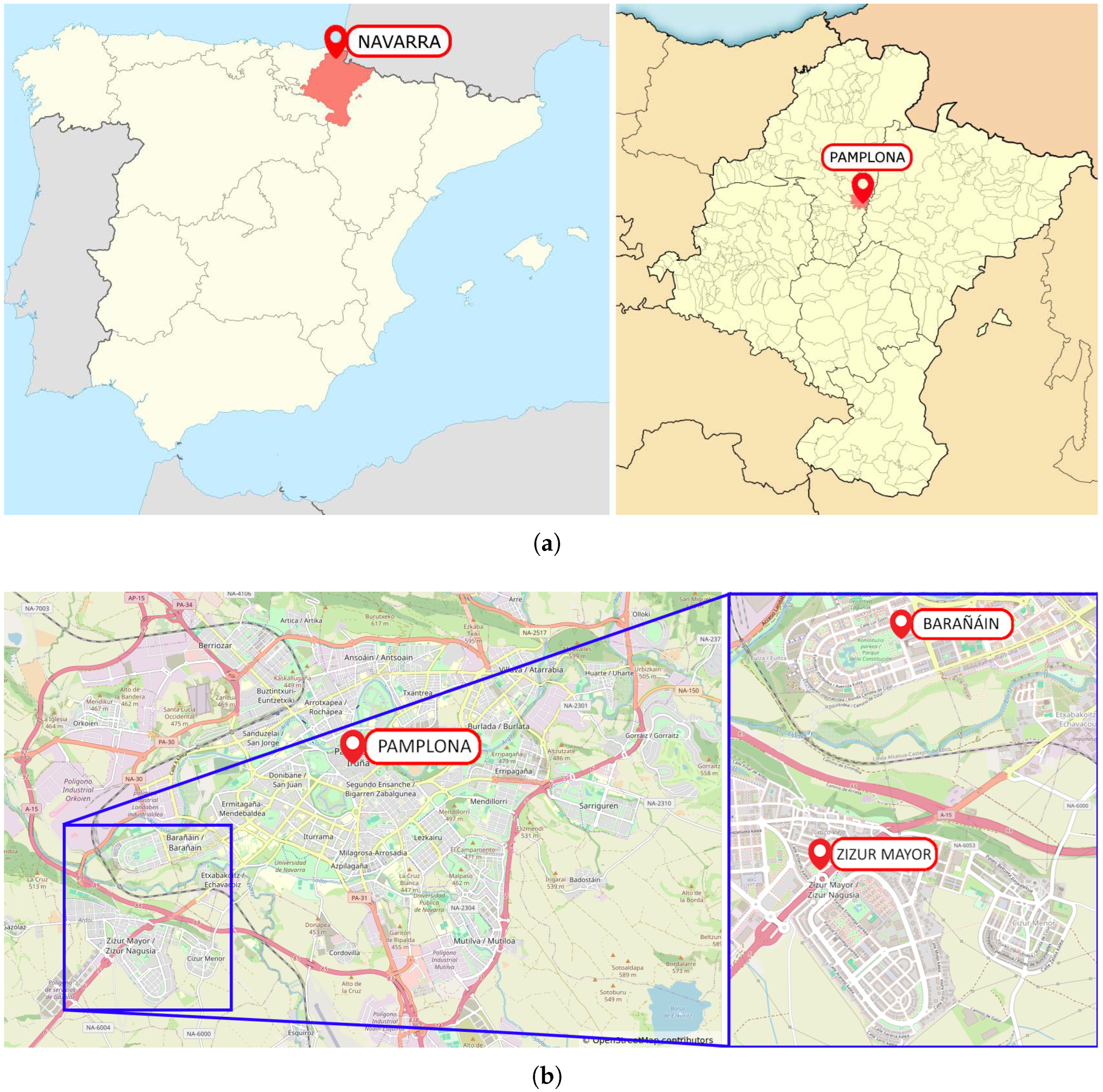
Figure 1. Case study location. (a) General view. Maps modified from WC1 (https://commons.wikimedia.org/wiki/File:Spain_2_location_map.svg; accessed on 30 June 2025) and WC2 (https://commons.wikimedia.org/wiki/File:Navarra-loc.svg; accessed on 30 June 2025). (b) Detailed view. Background map from OpenStreetMap (https://www.openstreetmap.org/copyright; accessed on 30 June 2025).
Water 17 02773 g001
Figure 2. Digital elevation models (DEMs), in the first column, and soil distribution maps, in the second column, for the Barañáin (a,b) and Zizur Mayor (c,d) case studies. Taken from [39].
Water 17 02773 g002
Figure 3. Spatial distribution of rainfall intensity (mm/h) at 10 min intervals during the observed event of 20 July 2010 for the Barañáin case study. Each panel represents the rainfall field at the indicated time, showing the temporal evolution and spatial variability of precipitation across the study domain. The grayscale bar (0–100 mm/h) indicates rainfall intensity values.
Water 17 02773 g003
Figure 4. The synthetic hyetographs considered in this study. The code PXX-DY in the legend stands for a hyetograph with a precipitation of XX mm and a duration of Y hours. The first row shows the hyetographs with left-skewed peak positions, the second row with centered peak positions and the third row with right-skewed peak positions. The first column includes the 1 h hyetographs, the second column the 2 h hyetographs and the third column the 3 h hyetographs.
Water 17 02773 g004
Figure 5. Methodological framework for the present work.
Water 17 02773 g005
Figure 6. Examples of results for the synthetic hyetograph with P = 60 mm, D = 1 h and a centered intensity peak (HCP60D1) in the Barañáin case study: maximum water depths (WDs) and flood extension (FE; white = flooded, black = dry) considering both infiltration models (GA and CN) and both hydraulic models (HEC-RAS and IBER). The first column shows the results for HEC-RAS and the second column for IBER.
Water 17 02773 g006
Figure 7. Examples of results for the synthetic hyetograph with P = 60 mm, D = 1 h and a centered intensity peak (HCP60D1) in the Zizur case study: maximum water depths (WDs) and flood extension (FE; white = flooded, black = dry) considering both infiltration models (GA and CN) and both hydraulic models (HEC-RAS and IBER). The first column shows the results for HEC-RAS and the second column for IBER.
Water 17 02773 g007
Figure 8. Comparisons of water depth distributions between the IBER and HEC-RAS hydraulic models for the 20 mm synthetic rainfall hyetograph before removing outliers (abnormal depth values obtained in HEC-RAS) in Barañáin (left) and Zizur (right).
Water 17 02773 g008
Figure 9. Locations of outliers (abnormal depth values obtained in HEC-RAS) in Barañáin (left) and Zizur (right).
Water 17 02773 g009
Figure 10. Distribution of positive (left) and negative (right) outliers in the water depth differences of HEC-RAS and IBER.
Water 17 02773 g010
Figure 11. Distribution of water depths between IBER and HEC-RAS for 20 mm synthetic rainfall hyetograph in Barañáin (left) and Zizur (right) after removing outliers.
Water 17 02773 g011
Figure 12. Comparison of maximum water depth between IBER and HEC-RAS models for the two infiltration methods (CN in grey and GA in black), applying two metrics for each rainfall event: RMSE values (top) and MAE values (bottom).
Water 17 02773 g012
Figure 13. Relationship between RMSE values and storm precipitation (left) and duration (right).
Water 17 02773 g013
Figure 14. Comparison of flooded area extents between IBER and HEC-RAS for the two infiltration methods using performance matrices. (TopBottom) SENS (sensitivity), miss rate, SPEC (specificity) and fall-out.
Water 17 02773 g014
Figure 15. Relationship between sensitivity values and event precipitation (left) and duration (right).
Water 17 02773 g015
Figure 16. Performance of both infiltration methods (GA and CN) on each hydraulic model (IBER and HEC-RAS). (TopBottom) SENS, miss rate, SPEC and Fall-Out comparisons between IBER and HEC-RAS for the two infiltration methods.
Water 17 02773 g016
Table 1. Summary of data used for hydraulic model implementation, including source, resolution and application.
DataSourceResolutionApplication
Digital elevation model (DEM) [39]2 mTerrain, model geometry
CORINE Land Cover (CLC 2018) [39]10 mInfiltration model parameters (Green-Ampt, Curve Number)
Rainfall events (observed, distributed) [41]15 m and 10 min (1 raster/step)Rainfall events, boundary conditions for hydraulic model
Rainfall events (observed, point rainfall) [42]10 minRainfall events, boundary conditions for hydraulic model
IDF curves for Pamplona city [42]15 minSynthetic hyetographs, boundary conditions for hydraulic model
Table 2. Summary of settings for both hydraulic models.
SettingsHEC–RASIBER
Terrain and topographyDEM (2 m)DEM (2 m)
Geometry and meshQuadrilateral min. area 0.5 m2 avg. area 10 m2Triangular side length 2 m
Infiltration parametersValues proposed in [40], based on soil cover and land use
Roughness coefficientsManning coefficient based on soil cover and land use
Boundary conditionsRainfall events (see Table 1)
EquationsDiffusion waveShallow Water Equations (SWEs)
Table 3. Infiltration model comparison results for the Barañáin case study using HEC-RAS. GA is considered as the ground truth value. Abbreviations: RMSE = root mean square error; MAE = mean absolute error; Pre = precision; NPV = negative predictive value; Sens = sensitivity; Spec = specificity; Acc = accuracy.
EventRMSEMAEPreNPVSensMiss RateSpecFall-OutAcc
20JUL2010_21100.2700.0520.9740.9240.8230.1770.9900.0100.937
HCP20D10.1160.0100.9980.9730.5540.4471.0000.0000.974
HCP40D10.1510.0180.9940.9490.4900.5101.0000.0000.951
HCP60D10.1780.0260.9890.9350.5080.4930.9990.0010.938
HCP40D20.1480.0180.9950.9520.5070.4931.0000.0000.955
HCP60D20.1790.0260.9910.9370.5260.4750.9990.0010.940
HCP40D30.1500.0180.9950.9520.5090.4911.0000.0000.954
HCP60D30.1810.0260.9910.9360.5310.4690.9990.0010.940
HDP20D10.1230.0100.9970.9770.5750.4261.0000.0000.978
HDP40D10.1500.0170.9910.9570.5100.4901.0000.0000.958
HDP60D10.1760.0240.9860.9380.4940.5060.9990.0010.941
HDP40D20.1620.0250.9940.9180.3740.6261.0000.0000.922
HDP60D20.1800.0250.9870.9380.5310.4690.9990.0010.941
HDP40D30.1510.0180.9930.9550.5190.4811.0000.0000.956
HDP60D30.1820.0260.9870.9370.5280.4720.9990.0010.940
HIP20D10.1140.0100.9980.9730.5500.4501.0000.0000.974
HIP40D10.1500.0180.9950.9490.4880.5121.0000.0000.952
HIP60D10.2130.0260.8190.9730.8100.1900.9750.0250.954
HIP40D20.1460.0170.9970.9540.5080.4921.0000.0000.956
HIP60D20.1770.0250.9900.9380.5200.4800.9990.0010.942
HIP40D30.1500.0180.9950.9540.5230.4771.0000.0000.956
HIP60D30.1790.0260.9930.9380.5280.4721.0000.0000.942
Table 4. Infiltration model comparison results for the Barañáin case study using IBER. GA is considered as the ground truth value. Abbreviations: RMSE = root mean square error; MAE = mean absolute error; Pre = precision; NPV = negative predictive value; Sens = sensitivity; Spec = specificity; Acc = accuracy.
EventRMSEMAEPreNPVSensMiss RateSpecFall-OutAcc
20JUL2010_21100.1040.0410.9980.7850.1020.8981.0000.0000.790
HCP40D10.0200.0060.8130.9840.8370.1630.9810.0190.968
HCP60D10.0260.0090.9520.9650.8440.1560.9900.0100.963
HCP40D20.0220.0070.7170.9890.8550.1450.9740.0260.965
HCP60D20.0230.0090.9230.9730.8730.1270.9850.0160.965
HCP40D30.0240.0070.7130.9890.8710.1290.9720.0280.964
HCP60D30.0230.0090.9120.9750.8820.1180.9820.0180.964
HDP20D10.0430.0100.3800.9510.0440.9570.9960.0040.948
HDP40D10.0170.0060.8440.9780.7980.2020.9840.0160.966
HDP60D10.0270.0100.9610.9500.7970.2030.9920.0080.952
HDP40D20.0180.0060.7680.9830.8150.1850.9770.0230.963
HDP60D20.0260.0100.9480.9620.8400.1600.9890.0110.959
HDP40D30.0180.0060.7710.9830.8180.1820.9770.0230.963
HDP60D30.0250.0100.9480.9620.8420.1580.9890.0110.960
HIP40D10.0210.0060.7620.9880.8540.1460.9770.0230.968
HIP60D10.0240.0090.9230.9760.8770.1230.9860.0150.968
HIP40D20.0240.0070.6410.9930.8800.1200.9710.0290.966
HIP60D20.0260.0070.8640.9850.9070.0930.9760.0240.966
HIP40D30.0290.0080.6260.9940.9040.0960.9680.0320.965
HIP60D30.0330.0080.8450.9860.9160.0840.9720.0280.964
Table 5. Infiltration model comparison results for the Zizur case study using HEC-RAS. GA is considered as the ground truth value. Abbreviations: RMSE = root mean square error; MAE = mean absolute error; Pre = precision; NPV = negative predictive value; Sens = sensitivity; Spec = specificity; Acc = accuracy.
EventRMSEMAEPreNPVSensMiss RateSpecFall-OutAcc
St2_20190.0720.1430.7240.9730.9730.0270.7210.2790.829
St2_20100.0960.2070.8940.9580.9800.0200.7980.2020.913
St1_20190.0560.1180.6020.9920.9840.0160.7530.2470.816
St1_20100.0490.1190.4590.9990.9960.0040.7980.2020.827
HIT200P60D10.0640.1170.8360.8470.8410.1590.8430.1570.842
HIT100P60D30.1010.1710.6620.9690.9770.0230.5880.4120.764
HIT100P60D20.0990.1670.6490.9650.9730.0270.5920.4080.758
HIT020P40D10.0710.1360.5240.9960.9930.0070.6890.3110.767
HIT010P40D30.0920.1550.5630.9860.9850.0150.5930.4070.729
HIT010P40D20.0880.1540.5430.9860.9830.0170.6010.3990.725
HIT002P20D10.0250.0650.8140.9410.8440.1560.9280.0720.905
HDT200P60D10.0550.1110.6250.9860.9760.0240.7430.2570.814
HDT100P60D30.0780.1420.6630.9380.9400.0600.6560.3440.775
HDT100P60D20.0770.1370.6660.9330.9350.0650.6580.3420.775
HDT020P40D10.0490.1070.5330.9940.9840.0160.7620.2380.810
HDT010P40D30.0640.1200.5740.9650.9450.0550.6870.3130.767
HDT010P40D20.0680.1290.9370.6650.9370.0630.6650.3350.703
HDT002P20D10.0450.1160.3830.9990.9960.0040.8130.1870.832
HCT200P60D10.0740.1370.6290.9910.9880.0120.6820.3180.790
HCT100P60D30.1030.1740.6740.9530.9670.0330.5840.4160.764
HCT100P60D20.0970.1670.6680.9590.9680.0320.6090.3910.770
HCT020P40D10.0700.1360.5430.9950.9900.0100.6950.3050.774
HCT010P40D30.0900.1560.5840.980.9780.0220.6100.3900.742
HCT010P40D20.0850.1500.5580.9810.9760.0240.6140.3860.735
HCT002P20D10.0610.1330.3570.9990.9970.0030.7390.2610.772
Table 6. Infiltration model comparison results for the Zizur case study using IBER. GA is considered as the ground truth value. Abbreviations: RMSE = root mean square error; MAE = mean absolute error; Pre = precision; NPV = negative predictive value; Sens = sensitivity; Spec = specificity; Acc = accuracy.
EventRMSEMAEPreNPVSensMiss RateSpecFall-OutAcc
St2_20100.1010.0330.3430.9990.9960.0040.8920.1080.898
HIT200P60D10.0720.0180.4170.9970.9200.0800.9500.0500.949
HIT100P60D30.1100.0280.4460.9950.9260.0740.9300.0700.929
HIT100P60D20.1020.0270.4310.9950.9210.0790.9290.0710.929
HIT020P40D10.0730.0200.3130.9980.9350.0650.9430.0570.942
HIT010P40D30.0790.0200.2600.9990.9610.0390.9480.0520.948
HIT010P40D20.0750.0190.2620.9990.9570.0430.9490.0510.949
HDT200P60D10.0410.0110.6580.9910.8790.1210.9680.0320.963
HDT100P60D30.0510.0120.6470.9950.9290.0710.9650.0350.963
HDT100P60D20.0500.0120.6450.9950.9270.0730.9650.0350.963
HDT020P40D10.0450.0150.2990.9950.8580.1420.9380.0620.936
HDT010P40D30.0550.0170.2970.9960.8860.1140.9370.0630.936
HDT010P40D20.0540.0170.2900.9960.8840.1160.9370.0630.936
HCT200P60D10.0610.0150.5780.9940.9030.0970.9600.0400.957
HCT100P60D30.0830.0190.5230.9950.9200.0800.9540.0460.952
HCT100P60D20.0740.0180.5200.9950.9170.0830.9550.0450.953
HCT020P40D10.0690.0200.3330.9970.9190.0810.9390.0610.939
HCT010P40D30.0760.0210.3050.9980.9280.0720.9400.0600.940
HCT010P40D20.0730.0200.2980.9980.9260.0740.9410.0590.941
Disclaimer/Publisher’s Note: The statements, opinions and data contained in all publications are solely those of the individual author(s) and contributor(s) and not of MDPI and/or the editor(s). MDPI and/or the editor(s) disclaim responsibility for any injury to people or property resulting from any ideas, methods, instructions or products referred to in the content.