Abstract
Mining-induced surface subsidence is a typical geological hazard. Loose layer drainage disturbed by coal mining can exacerbate surface subsidence in terms of both the extent and amount, thereby increasing the risk of building deformation and environmental degradation in mining areas. However, currently the prediction results of surface subsidence considering these two factors are not precise enough, which contradicts the principles of green coal mining. Firstly, this paper introduces the probability integral method, which predicts mining-induced surface subsidence. Subsequently, based on the soil–water coupled theory and the derived characteristic curve of groundwater level decline, a surface subsidence prediction model that considers loose layer drainage is constructed using triple integral transformation. Finally, a more precise surface subsidence prediction model considering both factors is proposed based on the principle of superposition. The model is applied to the mining of working panel 1309 in Shanxi province, China, an area rich in coal yet scarce in water resources. When compared with the measured subsidence data, the proposed model achieves a root mean square error (RMSE) of 27 mm, while the RMSEs of existing models are 78 mm and 123 mm, respectively. The prediction accuracy has been significantly improved. In addition, the proposed model is further validated through fluid–solid coupling numerical calculations in FLAC3D. The subsidence results considering the single effect of each factor also demonstrated good validation accuracy. Overall, the proposed model can accurately describe the surface subsidence considering both factors. This research can provide a theoretical guide for assessing the environmental impact and building damage, while contributing to the sustainable development of land use and groundwater resource in mining areas.
1. Introduction
Coal serves as a primary basic energy source and vital industrial raw material in China. Despite the decrease in its consumption proportion amidst the backdrop of “carbon peaking” and “carbon neutrality” goals, coal remains the mainstay of China’s energy mix, given the country’s distinct energy resource endowment characterized by “scarcity of oil and natural gas, but relative abundance of coal”. However, underground coal mining disrupts the stress equilibrium around the mining site, leading to varying degrees of movement, deformation, and damage in the rock strata. The damage in the rock strata also depends on the damage to minerals that constitute the rock [1]. Due to the deformation and damage of rock strata, the soil located above the rock strata also undergoes movement and deformation, ultimately giving rise to surface subsidence. Mining-induced surface subsidence can trigger ground fissures [2,3] and cracking of buildings [4], impair the functionality of infrastructure, and pose serious risks to ecological security and the sustainable development of mining areas [5].
During the process of coal mining, the deformation and cracking of rock strata render the originally impermeable rock layers permeable to water. When the overlying rock strata contain Quaternary or Tertiary aquifers, groundwater flows into the mined-out area through the rock fractures, causing a decline in the groundwater level and subsequently leading to compression of the loose layer and surface subsidence [6], as shown in Figure 1a. Therefore, the loose layer plays a significant role in mining subsidence [7]. The extent of surface subsidence caused by groundwater level decline are typically greater than those induced by coal mining [8], sometimes affecting areas hundreds of meters away and leading to significant movement and deformation even in areas not directly influenced by mining activity [9]. For example, studies on eight working panels across two coal mines in southern Illinois revealed that the maximum mining influence angle (or angle of draw) for deep groundwater can reach 60° [10]. Literature [11] monitored the surface subsidence resulting from long-term groundwater pumping and drainage at a mine, finding a decline in groundwater level exceeding 50 m and maximum stratigraphic compression exceeding 300 mm. The subsidence amount also caused varying degrees of damage to the surrounding buildings and structures. It is evident that although the surface subsidence induced by loose layer drainage may not be significant, the damage it triggers cannot be overlooked. This not only poses serious safety hazards to infrastructure around the mining site but also complicates the surface subsidence prediction due to the increase in factors. Therefore, in-depth research is needed on surface subsidence induced by coal mining and loose layer drainage.
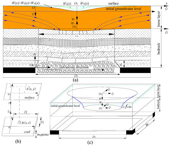
Figure 1.
(a) A surface subsidence model considering both the effects in a two-dimensional condition. The black subsidence curve W (x) is the model considering both the effects. The green subsidence curve Wc (x) is the model considering the single effect of coal mining. The cyan subsidence curve Ww (x) is the model considering the single effect of loose layer drainage. The blue curves with blue arrows represent the groundwater level decline direction; (b) three-dimensional coordinate system of PIM; (c) loose layer drainage region in the three-dimensional coordinate system.
Mining-induced disturbances alter the hydraulic properties of aquifers during the process of groundwater level decline. Significant groundwater loss due to coal mining produces a localized drop in the water head around the mined-out area, forming a funnel-shaped depression [12,13]. The loose layer drainage can thus be regarded as a process of large-scale groundwater extraction, akin to a massive pumping well [14]. Conventionally, the groundwater depression cone generated by pumping is understood as a “funnel-shaped zone of water head decline” [15,16]. In recent years, researchers have explored the patterns of groundwater level changes under the mining-induced disturbance. In terms of practical measurements, Chambers et al. (2015) [17] proposed the use of automated time-lapse electrical resistivity tomography to monitor groundwater. Field observations have revealed that images of resistivity changes and direct current conductivity (DGC) results are highly useful for determining pre-rebound groundwater levels, which closely match the groundwater levels in observation wells. Additionally, they can identify peak groundwater levels that are in good agreement with surface observations. In terms of simulation studies, Li conducted similar material simulation experiments considering two scenarios: coal mining advancing perpendicular to, and parallel with, the direction of groundwater flow. By analyzing the data on water level changes, he used Surfer (version 12) software to visually reconstruct the changes in groundwater decline and the influence boundary under the mining condition. As the working panel advances further, the influence radius and the decline depth of groundwater increase, with the degree of groundwater level decline being inversely proportional to the distance from the working panel [18]. Loupasakis, through a literature review, found that subsidence funnels caused by dewatering under the influence of opencast mining can extend for several kilometers. He used PLAXIS 2D (version 8) finite element simulation to explain the mechanisms considering different deformations and surface cracks within the subsidence funnel area [11]. Khan applied the visual MODFLOW (version 2011.1) model to groundwater level data, revealing that coal mining has impacted the groundwater resources, with groundwater levels declining at a rate of 0.142 m per year [19]. Pan established a groundwater flow system model for abandoned mine areas and used the MODFLOW calculation module in GMS (Groundwater Model System, version 7.0) to study the regional groundwater flow field. The study found that before the coal mine was closed, several funnels formed in the mining area, with central water levels below −25 m. After the mine was closed, the original drainage systems ceased operation, leading to a gradual recovery of groundwater levels and a reduction in the funnels. The rate of groundwater level recovery slowed as the time since mine closure increased [13]. Although these studies provide valuable insights into groundwater level variation under mining disturbances, the quantitative description of the spatial distribution of groundwater levels remains inadequate. To further analyze the quantitative relationship between groundwater level changes and soil deformation, it is necessary to determine the spatial distribution of groundwater level within the loose layer under the mining disturbance. This will pave the way for the accurate prediction of surface subsidence.
In research addressing surface subsidence caused by both coal mining and loose layer drainage, Liu applied the theory of random media to superimpose the drainage-induced subsidence with mining-induced subsidence, thereby deriving a formula for calculating surface subsidence and deformation caused by opencast excavation and drainage [20]. Tang and Yuan summarized and analyzed the laws of surface movement under thick collapsible loess through numerical simulation and field observations, respectively, and established a calculation model for additional subsidence caused by water loss in the mining-affected loess layer [21,22]. Li employed FLAC3D (version 3.0) numerical simulation software to examine the displacement field and seepage field within the overlying strata. His results indicated that the maximum subsidence increased by about 7% when groundwater was present [23]. Subsequently, he constructed a calculation model for soil compression in both phreatic and confined aquifers under coal mining in thick alluvial formations. Through analysis of the model parameters, it was found that the soil compression in the phreatic aquifer exhibited a parabolic growth relationship with the decline of groundwater level, while the soil compression in the confined aquifer showed a linear growth relationship [24]. Chen incorporated drainage effect in her research on mining subsidence, proposing a calculation model and control theory for surface subsidence considering these two factors [25]. Starting from the subsidence mechanism in the mining area with thick alluvial formations, Zhou combined the internal deformation characteristics of soil and rock masses and applied soil mechanics and mining subsidence theories to establish a prediction model that takes the thick alluvial layer into account through the principle of superposition [26]. Despite these contributions, most studies on drainage-induced subsidence have been limited to two-dimensional plane conditions, with insufficient exploration in three-dimensional contexts. Additionally, existing studies are unable to quantitatively capture the observed phenomenon where surface subsidence caused by groundwater level decline typically has a larger subsidence extent. Therefore, there is a pressing need to develop a more precise mathematical model to reveal both the effects of coal mining and loose layer drainage in three-dimensional space, and to explain the phenomenon where although the amount of stratigraphic subsidence induced by loose layer drainage is relatively small in a mining area, its spatial influence area is extensive.
Shanxi province is a major coal-producing region in China. Meanwhile, as Shanxi belongs to the North China region, it experiences an arid climate and a severe shortage of water resources (with per capita water resources of less than 400 cubic meters) [27]. Significant surface subsidence occurs in the province, primarily driven by coal mining and the associated loose layer drainage [28]. Based on the theory of random media, the probability integral method (PIM) is induced to predict surface subsidence considering the single effect of coal mining. Subsequently, based on the soil–water coupled deformation equations and the derived characteristic curve of groundwater level decline, a surface subsidence prediction model that considers loose layer drainage is constructed using triple integral transformation. Finally, a more precise prediction model for surface subsidence accounting for both the effects of coal mining and loose layer drainage is established using the superposition principle. Taking the mining of working panel 1309 in Shanxi province as a case study, this paper verifies that the proposed model can accurately describe the surface subsidence in the mining area. Furthermore, the proposed model is further validated through fluid–solid coupling numerical calculations in FLAC3D. When considering the single effect of each factor, the simulated subsidence values show little discrepancy from those calculated by the proposed model, and the trends of subsidence value changes along each observation line are consistent, which once again demonstrates the scientific validity of the proposed model. This paper also conducts a quantitative analysis of the impact of parameter variations in the model on the subsidence prediction results. The research can provide more accurate results for predicting surface subsidence affected by coal mining and loose layer drainage. It offers scientific guidance for assessing the environmental impact and building damage in mining subsidence areas.
2. Surface Subsidence Prediction Model Considering Both the Effects of Coal Mining and Loose Layer Drainage
As shown in Figure 1a, a surface subsidence prediction model due to coal mining under the condition of a water-bearing loose layer is established. In order to explain the combined mechanism of coal mining and loose layer drainage in a more intuitive manner, we will describe it in the context of a two-dimensional-plane condition.
During the process of establishing the mathematical model in this paper, for the convenience of modeling, two-dimensional and three-dimensional coordinate systems are defined (xOz, sOczc, Oxyz, and so on, as in Figure 1). The definitions and functions of each coordinate system are elaborated in Appendix A.1.
Both underground coal mining and drainage in the loose layer contribute to surface subsidence, with the total deformation potentially approximated as the linear superposition of individual subsidence components, as shown in Figure 1a (W(x) = Wc(x) + Ww(x)).
2.1. Surface Subsidence Prediction Model Considering the Single Effect of Coal Mining
In China, the probability integral method (PIM) is a most widely used surface subsidence prediction method, and it is named after the probability integrals contained in the formulas used for predicting mining-induced movement and deformation [29]. It is also the officially recommended model for mining subsidence prediction [30]. The PIM idealizes the rock strata affected by coal mining as a loose medium, treating the movement of rock strata as a stochastic process.
It can be assumed that the change in void volume after mining is the process that triggers surface subsidence based on the influence function theory [31,32] and according to the principle of superposition [29,33]. As shown in Figure 1b, for a rectangular mining area (a working panel) the mining length along the strike direction (x-axis) is D3, and the mining length along the dip direction (y-axis) is D1. The subsidence at point A is as follows:
where r is the main influence radius (m), r = H/tanβ; H is the average mining depth (m); β is the main influence angle (◦); θ0 is the mining influence propagation angle (◦); w0 = mcqcosα is the surface maximum subsidence (mm); mc is the thickness of the coal seam (mm); q is the subsidence coefficient; and α is the dip angle of the coal seam (°). The specific expressions of Equation (1) can be found in Appendix A.2.
Equation (1) or the specific expressions from Equations (A1)–(A3) are the PIM in a three-dimensional coordinate system Oxyz, which predicts the mining-induced surface subsidence.
2.2. Surface Subsidence Prediction Model Considering the Single Effect of Loose Layer Drainage
During drainage in a water-bearing loose layer, the stress originally borne by the pore water is transferred to the solid soil particles, leading to an increase in effective stress and causing compression of the loose layer [34]. Due to the different degrees of water head drop at different locations within the drainage area the rates and amounts of pore pressure dissipation vary, which in turn results in uneven subsidence of the overlying loose layer, as illustrated by the subsidence curve (Ww (x)) in Figure 2.
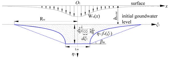
Figure 2.
Surface subsidence curve considering loose layer drainage and characteristic curve of the groundwater level decline.
2.2.1. The Characteristic Curve of the Groundwater Level Decline
As shown in Figure 2, before drainage the groundwater level is at η1 = hw-ini. During the surface subsidence induced by groundwater level decline, the characteristic curve (the drainage boundary) is denoted as the blue curve in Figure 2. The influence radius of loose layer drainage is Rw.
The black curve (Ww (x)) in Figure 2 is the surface subsidence model caused by loose layer drainage in a two-dimensional plane condition, which is the foundation of the model for predicting the surface subsidence caused by loose layer drainage in a three-dimensional coordinate system. The modeling process is shown in Appendix A.3.
In Figure 2, η1 = fw(ξ1) is the characteristic curve of the groundwater level decline due to loose layer drainage. It can be represented as a combination of two curves and a straight line as follows: f1w (−Rw ≤ ξ1 ≤ −Lw/2), f2w (−Lw/2 < ξ1 < Lw/2), f3w (Lw/2 ≤ ξ1 ≤ Rw). The expression of fw(ξ1) is:
The derivation process of Equation (2) is elaborated in Appendix A.4.
2.2.2. Surface Subsidence Predicting Model Caused by Loose Layer Drainage in a Three-Dimensional Coordinate System
When a working panel is mined, according to the model establishment process of PIM in Section 2.1 and Appendix A.2 combined with the surface subsidence Ww (x) in Appendix A.3, the surface subsidence prediction model Ww (x, y) in O1ξ1ζ1η1 is as follows:
Analogous to the integration region of a curved trapezoid (the shaded region in Figure 2) in Equation (A11), the drainage region Ωw in the O1ξ1ζ1η1 three-dimensional coordinate system is a curved-edge elliptical frustum, as shown in Figure 1c. The boundaries of the drainage region Ωw are defined in Appendix A.4.
The upper limit of integration for η1 is a piecewise function (η1 = fw(ξ1) in Equation (2)), making it somewhat complex. If we follow this sequence of integration, namely integrating first with respect to ξ1, then with respect to ζ1, and finally with respect to η1, to obtain the subsidence value in Equation (3) then the integration process will be difficult, and it may even be impossible to obtain the final integrated value. The reasons for the complexity of this integration are as follows:
- (1)
- The integrand lacks an elementary function, necessitating the use of numerical integration methods for the solution.
- (2)
- In the ξ1O1ζ1 plane, the integration region is an ellipse, and the expression for ζ1 in terms of ξ1 is also complex due the complexity of the ellipse function in a Cartesian coordinate system.
- (3)
- In the ξ1O1η1 plane, η1 is a piecewise function of ξ1 (Equation (2)), and the expressions for the piecewise function are also complex (the first and third equations in Equation (2)). Now, in the O1ξ1ζ1η1 three-dimensional coordinate system, η1 is inevitably a piecewise function of both ξ1 and ζ1. Simultaneously, ζ1 is also a function of ξ1. More crucially, in the ξ1O1η1 or ζ1O1η1 plane, rw and Rw are constants, whereas in the O1ξ1ζ1η1 three-dimensional coordinate system, rw and Rw are variables in the region of integration which is a curved-edge elliptical frustum. Expressions representing the upper and lower limits of integration are difficult to represent explicitly using functional notation.
To solve this triple integral, the current literature mostly simplifies the characteristic curve of the groundwater level decline into a straight line for integration (the blue-dot lines in Figure 2) [35,36]. Although this approach can yield an integral result, it leads to an overestimation of the final value because the integration region is enlarged. In the context of precision coal mining [37], overestimating the integral result is inappropriate.
In this paper, based on the shape characteristics of the integration region Ωw in Figure 1c and the theory of calculus [38], by changing the order of integration we can express ξ1 and ζ1 as functions of η1, thereby enabling accurate calculation of the triple integral.
The triple integral (Equation (3)) within the region of the curved-edge elliptical frustum Ωw can be explicitly expressed as:
where ξ1 = a(η1) is a function of ξ1 with respect to η1. ζ1 = b(η1, ξ1) is a function of ζ1 with respect to η1 and ξ1. Within the region of integration Ωw, at any position along the η1-axis, an ellipse with a semi-major axis of length a(η1) and a semi-minor axis of length b(η1) is formed in the ξ1O1ζ1 plane.
Based on the analysis in Section 2.1 and Section 2.2, the proposed model is W(x, y) = Wc(x, y) + Ww(x, y). For a rectangle working panel, Wc(x, y) is from Equations (A1)–(A3), and Ww(x, y) is Equation (4).
3. Background of the Study
3.1. Study Area
Working panel 1309 is located in Changzhi City, Shanxi province, China, as illustrated in Figure 3. The mining parameters and related information for this panel are presented in Table 1.
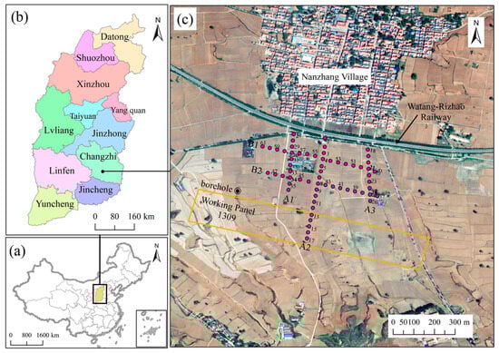
Figure 3.
(a) Map of China; (b) map of Shanxi province; (c) the geographic location of working panel 1309. The magenta-circle dots represent the observation points used for leveling. The orange polygon represents the working panel 1309.

Table 1.
Mining information of working panel 1309.
3.2. The Engineering Geological Condition of Rock Strata
The panel is designed to mine 3# coal in the Shanxi Formation. The roof is mainly mudstone and siltstone. The stratigraphic column is shown in Figure 4. The drilling location is close to the northwest corner of the panel, which is shown in Figure 3.
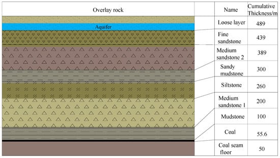
Figure 4.
Borehole-based lithological columnar section.
3.3. Layout of Observation Points and Observation Water Wells
To investigate the impact of the surface subsidence due to the mining of working panel 1309 on Watang–Rizhao Railway (Figure 3), a monitoring system was established. A total of 61 points (magenta-circle dots in Figure 3) were arranged in five observation lines (two transverse and three longitudinal). Structured monitoring was conducted with consistent precision throughout the mining operation.
Jincheng Mining Industry Group also constructed 12 dedicated groundwater monitoring wells. The hydrological monitoring results (Table 2) reveal a groundwater level ranging from 0.75 m to 16 m, as determined through field surveys. Figure 5 illustrates the spatial distribution of villages hosting these monitoring wells.
Table 2.
Groundwater level monitoring results.
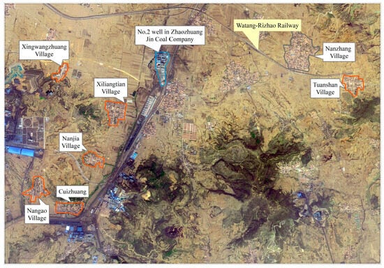
Figure 5.
The distribution of villages.
Considering both the historical monitoring data and the completion of mining operations on this panel (August 2016), the groundwater level benchmark was established at a burial depth of 10 m. Accordingly, the value of hw-ini in Section 2.2 is taken as 10.
3.4. The Geological Conditions of the Soil Layer
(1) Tertiary System (N)
The Pliocene Series (N2) of the Tertiary System features soil layers with a thickness ranging from 0 to 5 m, averaging approximately 3 m. These layers are primarily composed of brownish-red and brownish-reddish clay and sub-clay. It is in unconformable contact with the underlying strata.
(2) Quaternary System (Q)
① Middle Pleistocene (Q2)
The Middle Pleistocene Series has a thickness ranging from 5 to 15 m, with an average of about 10 m. It is characterized by its light reddish sandy clay, often containing calcareous concretions and sometimes intercalations of stone. This series is also in unconformable contact with the underlying strata.
② Upper Pleistocene (Q3)
Widely distributed in the region, the Upper Pleistocene Series has a thickness of 23 to 41 m, averaging approximately 31 m. Its dominant lithology is light yellow to brownish-yellow sandy clay, often interspersed with calcareous concretions and characterized by well-developed pores.
③ Holocene (Q4)
With a thickness ranging from 0 to 20 m, averaging around 8 m, the Holocene Series is composed of fine sand, silt, sandy soil, and gravel. It represents a set of recent alluvial deposits from riverbeds and diluvial deposits from the piedmont zone.
3.5. The Hydrological Conditions of Soil
① Quaternary Holocene and Upper Pleistocene porous aquifer
The aquifer consists of sand and gravel layers, with a water level depth of 0 to 14 m. The specific yield of water from boreholes is 0.7 to 11 m3/(h·m), and it mainly receives recharge from rainfall.
② Quaternary Middle Pleistocene porous aquifer
This layer is widely distributed in basins and hills. It has a thickness of 3 to 40 m. The aquifer is composed of red soil interspersed with calcareous concretions, representing a special type of clay fissure aquifer. It is the main aquifer for supplying water to farmland and for human and livestock consumption in Changzhi. The water level depth is 5 to 10 m, and the specific yield of water is 0.72 to 3.6 m3/(h·m).
③ Quaternary Lower Pleistocene porous aquifer
This layer is mainly distributed in the Changzhi basin and consists of a suite of variegated clay layers deposited in a lacustrine environment. The aquifer is composed of silty-fine sand lenses, with a total thickness of 5 to 40 m. Due to poor recharge conditions, it has weak water abundance and poor water quality.
④ Upper Tertiary Yushe Formation porous aquifer
This layer primarily consists of sand and gravel aquifers, with a water level depth of 8 to 15 m. The specific yield of water varies from 1.5 to 7.2 m3/(h·m).
4. Results and Discussion
4.1. Validation of the Proposed Model Based on Measured Data
The prediction effectiveness of the proposed model is validated based on the measured subsidence data from 61 observation points arranged above working panel 1309 and on the south side of the Watang–Rizhao Railway (in Figure 3).
The parameters of PIM (Wc(x, y)) include the subsidence coefficient q, the main influence angle tangent tanβ, the mining influence propagation angle θ0, and the inflection point offsets si (i = 1, 2, 3, 4). The values of these seven parameters are listed in Table 3, which are obtained from “The 1309 working panel surface and rock movement impact report”. This report is provided by Jincheng Mining Industry Group.
Table 3.
Values for the prediction parameters of PIM.
According to Equations (A2) and (A3), the values of other parameters in the proposed model Wc(x, y) are as follows: the main influence radius r is 157 m, the strike computed length l is 863 m, and the strike computed length L is 88 m.
The parameters of the proposed model Ww(x, y) include the height from the final groundwater level in the “large diameter well” to the bottom interface of the loose layer hw0, the height from the initial groundwater level to the bottom interface of the loose layer (or the thickness of the aquifer) Hw, the influence angle tangent due to soil drainage tanβw, the uniform water head decline length Lwξ and Lwζ, the initial groundwater level hw-ini, the coefficient of compaction av, the bulk density of pore water γw, and the initial porosity ratio of soil e0.
According to “The 1309 working panel surface and rock movement impact report”, coal mining of this panel has caused groundwater in the loose layer to flow towards the mined-out area. The groundwater directly above the mined-out area has been completely drained, thus hw0 can be set to 0 m. Based on the content in Section 3.3 and Table 2, the initial groundwater level hw-ini is 10 m. Considering the columnar diagram of rock layers shown in Figure 4, the thickness of the loose layer is 50 m. This means Hw is 50 − 10 = 40 m. Since the overlying strata in the study area consist of hard rock formations, and according to the values listed in Table A1, the parameters in Equation (A13) are assigned as c1 = 2.1, c2 = 16, and c3 = 2.5, respectively. Then the height of the caved rock Hk is 22.7 m. Based on the simulation experiment results from coal mining in the adjacent mining areas of the Zhaozhuang No. 2 mine field [39], the caved angles of αK1 and αK2 are both equal to 50°. For the mining length D3 of 935 m, Lwξ is 897 m. For the mining width D1 of 159 m, Lwζ is 120 m. The influence angle tangent due to soil drainage tan βw is 0.17. Taking into account that the loess in Shanxi province belongs to medium-compressibility soil, the coefficient of compaction av is 0.2 MPa−1. The bulk density of pore water γw is 9.81 kN/m3. The initial porosity ratio of soil e0 is 0.55. The parameters of Ww(x, y) about working panel 1309 along the ξ1O1η1 plane are shown in Figure 6.
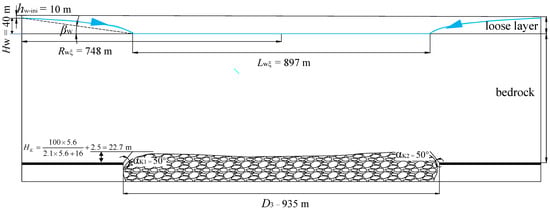
Figure 6.
The parameters schematic diagram of Ww(x, y) about working panel 1309 along the ξ1O1η1 plane. The blue curve with an arrow is the characteristic curve of the groundwater level decline. The blue straight line is the uniform water head decline region.
The surface subsidence prediction results obtained by substituting the values of the aforementioned parameters into the model proposed in this paper (equations from Equations (A1)–(A3) and Equation (4)) are shown in Figure 7. For the triple integral in Equation (4)), code was written and combined with numerical integration functions in MATLAB software (version R2022b) to perform calculations [40].
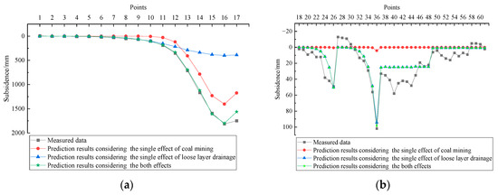
Figure 7.
Comparison between the measured data and the prediction values: (a) comparison of subsidence results from Points No. 1 to No. 17; (b) comparison of subsidence results from Points No. 18 to No. 61. Positive values represent subsidence, while negative values represent uplift.
As shown in Figure 7, the proposed model demonstrates a high degree of consistency between the prediction and measured subsidence values along Lines A1, A2, and A3. Specifically, on Line A2 (No. 1 to No. 17) the measured maximum subsidence reached 1813 mm at Point No.16, whereas the model predicted 1801 mm. On Line A1 (Points No. 27 to No. 36) the maximum measured subsidence was 102 mm at Point No. 36, compared with a predicted value of 98 mm. Similarly, on Line A3 (Points No. 18 to No. 26) the measured maximum subsidence was 49 mm at Point No. 26, while the predicted value was 50 mm. In contrast, the fitting performance for Line B1 and Line B2 is relatively poor. It is believed that there was site construction in the vicinity of the observation points along Line B1 and Line B2 (shown in Figure 3). The observation points not only undergo subsidence due to coal mining and loose layer drainage but are also affected by the site construction, leading to unsatisfactory fitting effects.
For a more detailed comparison of the measured and predicted subsidence values along Lines A1, A2, and A3, the predicted subsidence values, calculated separately for the single effect of each factor using the proposed model, are presented in Table 4.
Table 4.
Comparison between the measured data and the prediction values.
The data presented in Figure 7 and Table 4 indicate that the points located outside working panel 1309 that exhibit notable subsidence (greater than 10 mm) are primarily influenced by looser layer drainage, rather than by coal mining.
According to regulations [30], the subsidence influence boundary is typically determined based on points where the subsidence exceeds 10 mm. The subsidence influence boundaries for each effect (coal mining and looser layer drainage) are determined based on both the measured subsidence data and the subsidence data predicted by the proposed model along Line A2, as shown in Table 4. Based on the measured data, the subsidence influence boundary is 218 m. When considering only the single effect of coal mining, the boundary is reduced to 70 m, showing a significant discrepancy. In contrast, when considering only the effect of loose layer drainage, the boundary extends to 205 m, which is close to the subsidence influence boundary determined by the measured data. These results highlight the necessity of accounting for loose layer drainage under the disturbance of coal mining. This is because during the process of coal mining, loose layer drainage can obviously increase the extent of surface subsidence due to the larger influence radius of drainage Rw.
4.2. Validation of the Proposed Model Based on Numerical Simulation
As discussed in Section 4.1, the proposed mathematical model is capable of precisely depicting surface subsidence resulting from both the impacts, offering accurate predictions for both the amount and extent of surface subsidence. However, the measured subsidence data (the black-square curves in Figure 7) only reflect the cumulative outcome of these two factors and cannot isolate the contribution of each individual factor. Consequently, the prediction results of Wc (x, y), which represent the single effect of coal mining, and Ww (x, y), which represent the single effect of loose layer drainage, in the proposed mathematical model cannot be quantitatively verified using the measured subsidence data. Meanwhile, the characteristic curve of the groundwater level decline derived in Section 2.2.1 also remains insufficiently verified. This characteristic curve determines the integration domain (Figure 1c) for calculating surface subsidence through integration in the proposed mathematical model. The accuracy of the integration region will, to a certain extent, affect the accuracy of the prediction results. Therefore, to further validate the scientific validity of the proposed mathematical model this section employs the fluid–solid coupling module in FLAC3D numerical simulation software to conduct a more in-depth analysis of surface subsidence considering both the effects. The FLAC3D numerical simulation was employed to thoroughly verify the surface subsidence and the spatial distribution patterns of groundwater level decline.
Combining the content of Section 2.2 for the condition of the loose layer containing groundwater, the surface subsidence caused by coal mining is primarily related to two aspects: the lithology of the overlying rock and soil, and groundwater seepage within the loose layer. The groundwater seepage during coal mining involves a complex process. Deformable rock and soil will deform or move under the action of fluid pressure and the gravity of overlying rock strata. Such deformation or movement, in turn, provides feedback that affects changes in the groundwater seepage, thereby altering the magnitude and distribution of fluid. Consequently, surface subsidence in this context results from the coupled interaction between the overlying rock stress field and the groundwater seepage field. Therefore, it is both necessary and meaningful to utilize the fluid–solid coupling module in numerical simulation software to simulate and validate the proposed mathematical model.
4.2.1. Establishment of the Numerical Model
This paper employs the FLAC3D (Fast Lagrangian Analysis of Continua in 3-Dimensions, version 6.0) software to conduct numerical simulation calculations on surface subsidence induced by coal mining and loose layer drainage, taking the mining operation of working panel 1309 as an engineering case study.
The fluid–solid coupling module integrated within FLAC3D is adept at simulating the movement of a single fluid through isotropic (or anisotropic) porous materials. By standard configuration, fluid flow within these porous media is governed by Darcy’s law, whereas the solid medium operates under the effective stress principle [34,41]. Based on the aforementioned two theories, the interaction between the mechanical deformation of rock and soil and pore water pressure can be realized. When considering both effects, the seepage mode (model configure fluid) is activated to perform fluid–solid coupling calculations in FLAC3D. To separately analyze the surface subsidence extent and amount caused by coal mining and loose layer drainage, the same overburden mechanical parameters, model boundary conditions, and the model convergence condition are employed. By deactivating the seepage mode (activating the mechanical mode) and considering only the numerical simulation of the overburden stress field, the surface subsidence considering the single effect of coal mining is obtained. By subtracting the subsidence values at the 61 observation points above working panel 1309 (Figure 3) obtained from the numerical simulation considering only the overburden stress field from those obtained from the fluid–solid coupling calculation, the resulting values represent the subsidence considering the single effect of loose layer drainage at these 61 observation points. Finally, by comparing the subsidence values caused by each single factor obtained from numerical simulation with those calculated by the proposed mathematical model (Wc (x, y) and Ww (x, y)), and visually presenting the spatial distribution of groundwater level decline in FLAC3D, the scientific validity of the mathematical model proposed in this paper is further verified.
Based on the mining dimensions of working panel 1309 in Table 1 and the thickness of overlying rock strata layers (Figure 4), boundary protective coal pillars of 960 m in the x-direction and 970 m in the y-direction were reserved to eliminate boundary effects. A numerical model measuring 2860 m in length, 2100 m in width, and 489 m in height was constructed. The model element size in the horizontal direction was set to 20 × 20 m, while the vertical element size was adjusted according to the thickness of each stratum. A total of 35,440 elements have been divided in this model. Given the small dip angle of the coal seam for working panel 1309 (Table 1), it was designed as a horizontal coal seam in the model, with a coal seam thickness of 5.6 m. The overlying strata were stratified according to the stratigraphic column (Figure 4), with the loose layer thickness set to 50 m and no aquitard included. Excavation of working panel 1309 commenced at x = 330 m and ceased at x = 1270 m. The range in the y-direction extended from y = 420 m to y = 580 m. The in situ stress in the numerical model was generated by the self-weight, with each stratum set as an isotropic medium. According to Section 3.3 and Table 2, the initial groundwater level was set 10 m below the surface. The displacement boundary conditions set for the numerical model were specified as follows: The top surface (located at z = 489 m) was left unconstrained, permitting movement in every direction. Conversely, the bottom surface (at z = 0 m) was fixed, preventing any displacement in all directions. Additionally, the sides (x = 0 m, y = 0 m, x = 2860 m, y = 2100 m) were restricted from horizontal displacement, yet allowed to move vertically along the z-axis. The constitutive model for rock mass mechanics was defined as the Mohr–Coulomb Model. Since groundwater seepage in the loose layer was the main concern, the loose layer was set as an anisotropic seepage model, while each rock stratum was set as isotropic. In the model, the pore pressure at the initial groundwater level (z = 479 m) was set to 0, whereas the pore pressure at the bottom (z = 0 m) was set to 4.79 MPa. The excavated elements were defined with a null constitutive model (zone cmodel assign null) and a null fluid seepage model (zone fluid cmodel assign null). The top and bottom surfaces of the model were designated as impermeable boundaries, while the surrounding boundaries are set as constant head boundaries to simulate lateral recharge. The initial model established in FLAC3D is shown in the left part of Figure 8. The numerical simulation parameters of each layer in the model were obtained from Jin Coal Company, as shown in the right part of Figure 8.
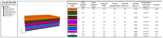
Figure 8.
Three-dimensional numerical simulation model.
4.2.2. Analysis of Numerical Simulation Results
- (1)
- Comparison of subsidence
According to Section 4.2.1, the subsidence contour map obtained from the numerical calculation of the overburden stress field considering the single effect of coal mining is shown in Figure 9a, while the subsidence contour map obtained from the fluid–solid coupling numerical calculation considering the both effects is depicted in Figure 9b.
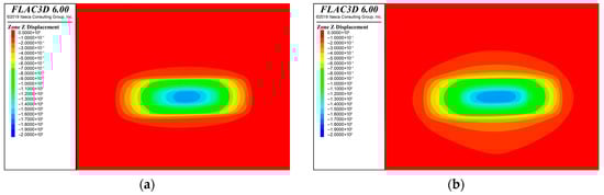
Figure 9.
Simulated subsidence contour maps: (a) considering the single effect of coal mining; (b) considering both the effects of coal mining and loose layer drainage.
As can be seen from Figure 9, the extent of surface subsidence is obviously larger when considering both the effects. Furthermore, the amount of surface subsidence is also increased (the area with larger subsidence values located at the center of the subsidence contour has expanded). The results of the numerical simulation are consistent with the conclusion derived from the proposed mathematical model calculations (Table 4), indicating that the loose layer drainage can increase both the amount and extent of surface subsidence.
When considering both effects, the simulated subsidence values for points from No. 1 to No. 17 are presented in Figure 10a, while those for points from No. 18 to No. 61 are shown in Figure 10b. Correspondingly, when considering the single effect of coal mining the simulated subsidence values for points from No. 1 to No. 17 are presented in Figure 10c, while those for points from No. 18 to No. 61 are shown in Figure 10d. Through subtraction operations, when considering the single effect of loose layer drainage the simulated subsidence values for points No. 1 to No. 17 are displayed in Figure 10e, while those for points No. 18 to No. 61 are shown in Figure 10f. For intuitive comparison, the subsidence values at all 61 points calculated using the proposed mathematical model for each single factor are also plotted in the corresponding figures of Figure 10, represented by blue-triangle curves, respectively.
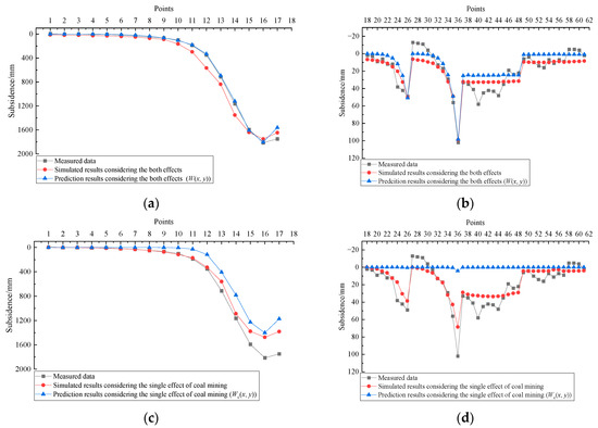
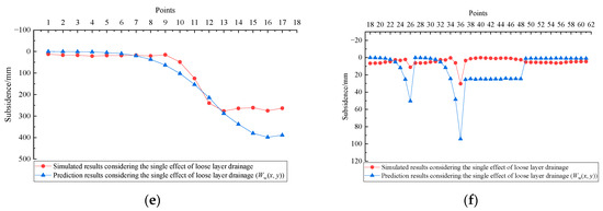
Figure 10.
Comparison of numerical simulation results (positive values means subsidence): (a) Points No. 1–17: both effects; (b) Points No. 18–61: both effects; (c) Points No. 1–17: single effect of coal mining; (d) Points No. 18–61: single effect of coal mining; (e) Points No. 1–17: single effect of loose layer drainage; and (f) Points No. 18–61: single effect of loose layer drainage.
In Figure 10a, the maximum simulated subsidence (at Point No. 16) reaches 1751 mm, closely aligning with the measured subsidence of 1813 mm. Similarly, in Figure 9b, the local maximum subsidence values at Points No. 26 and No. 36 are 47 mm and 99 mm in the simulation, which are near the measured values of 49 mm and 102 mm, respectively. The closeness of these simulated subsidence values to the measured ones underscores the accuracy of the numerical simulation results [42,43].
Focusing solely on the effect of coal mining, the simulated subsidence values for Points No. 16, No. 26, and No. 36 are 1475 mm, 36 mm, and 68 mm, respectively. Conversely, when considering only the effect of loose layer drainage, the simulated subsidence values for these points are 276 mm, 11 mm, and 31 mm, respectively.
As can be seen from Figure 10 and Table 5, although there are differences in specific values between the simulated and prediction results, the overall change trends of the subsidence curve under the influence of a single factor remain consistent. This consistency demonstrates the reliability of the numerical simulation results and also proves the scientific validity and accuracy of the proposed mathematical model. The main reason for the discrepancies between the results obtained by the two methods lies in their distinct theoretical foundations. The mathematical model is developed based on the stochastic medium theory, which belongs to the discontinuous medium theory, whereas the numerical simulation method is based on the finite difference method, which is classified as the continuous medium theory. These fundamental theoretical differences account for the variations in the calculation results.
Table 5.
Comparison between the simulated results and prediction results.
- (2)
- Analysis of the spatial distribution characteristics of groundwater level decline
The seepage flow vectors (black arrows) in the model cross-section (the symmetric plane of working panel 1309 at y = 500 m) and the horizontal plane (near the initial groundwater level, at z = 475 m) are shown in Figure 11.
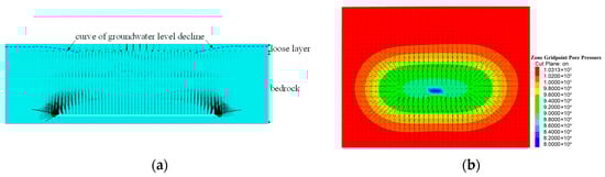
Figure 11.
Seepage vector distribution maps. (a) The seepage flow vectors at y = 500 m; (b) the seepage flow vectors at z = 475 m.
As can be seen from Figure 11a, after coal mining the overlying strata and loose layer undergo failure and deformation due to mining-induced disturbances, thereby forming seepage pathways that allow groundwater to flow into the mined-out area. The regions exhibiting the highest groundwater flow velocity are located around the coal seam and strata adjacent to the working panel, primarily concentrated within the plastic zones where rock strata have experienced failure, as seen in Figure 12b. The shape of groundwater level decline curves (blue dashed lines in Figure 11a) is similar to that derived from Equation (A21) (Figure A3), indicating the correctness of the groundwater level decline curve equation obtained through theoretical derivation. As can be seen from Figure 11b, when groundwater in the loose layer seeps into the mined-out area, the distribution pattern of pore water pressure within the loose layer resembles a “depression funnel”. The lower pore water pressure in the center and higher pressure around the periphery within the loose layer are attributed to the fact that the soil directly above the mined-out area is the first to be disturbed by mining activities, leading to a decrease in pore pressure due to groundwater seepage towards the mined-out area. The contour map of pore water pressure exhibits a “nearly elliptical” shape, similar to the curve pattern in Figure A4 This further verifies the rationality and accuracy of the soil drainage region delineated in Figure 1c and analyzed in Section 2.2.
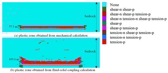
Figure 12.
Plastic zones distribution.
By comparing the plastic zones in Figure 12a,b, it can be observed that both zones exhibit a “saddle-shaped” distribution, characterized by higher on the sides and lower in the middle, a phenomenon consistent with the mining subsidence theory [29,33]. When considering only the overburden failure caused by coal seam mining, the developed height of the plastic zone (height of the water-conducting fracture zone [42,44]) is 57.5 m. However, when both coal mining and groundwater seepage are taken into account the developed height of the plastic zone increases to 105.6 m, indicating a significant expansion of the overburden failure area. Both heights of the water-conducting fracture zones fall within the range (45.23 m to 107.27 m) calculated in the literature [45], thereby confirming the accuracy of the numerical simulation results. This comparison of the plastic zones from the two numerical models demonstrates the necessity of considering groundwater effects during coal mining. This consideration is crucial for accurately determining the extent of mining-induced overburden damage and surface subsidence, as well as for protecting the ecological environment of the mining area.
4.3. The Advantages of the Model Proposed in This Paper
The existing surface subsidence prediction models considering both the effects mainly include two types.
The first type assumes that after soil drainage the differential subsidence caused by soil drainage will generate a movement dWwater(x) in the rock–soil mass above the affected element. For the overall surface subsidence, the differential subsidence will lead to movement (dWwater(x) + dWcoal(x)) in the rock–soil mass above the affected element (where dWcoal(x) represents the differential subsidence in the overlying rock considering the single effect of coal mining) [26,46,47]. The corresponding equation of the first existing prediction model is:
where Δe indicates the change in the void ratio of soil, and the other parameters are the same as previously defined.
The first existing prediction model can explain how loose layer drainage increases the amount of surface subsidence under the disturbance of coal mining. However, it fails to explain why loose layer drainage expands the extent of surface subsidence. This limitation arises because Ww(x) in Equation (5) adopts the main influence radius r (Equation (1)) from Wc(x) as a parameter, and there is no parameter for describing the influence radius of loose layer drainage to Ww(x). Therefore, the first existing model is insufficient for describing the expansion of the subsidence extent caused by loose layer drainage when predicting surface subsidence considering both the effects. The first existing prediction model was applied to calculate the subsidence of 61 points above working panel 1309. The result is shown in Figure 13 (the red-square curve). As shown in Figure 13, the subsidence values calculated by the first existing prediction model are generally underestimated. This underestimation is primarily because the model considers the influence radius of loose layer drainage Rw to be the same as the influence radius of coal mining r. In fact, r is smaller than Rw. As a result, when calculating the subsidence at the boundary the effect of loose layer drainage is not fully considered, leading to smaller prediction subsidence, especially at Points No. 26 and No. 36.
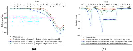
Figure 13.
Comparison among the prediction models considering both the effects: (a) comparison of subsidence results for Points No. 1–17; and (b) comparison of subsidence results from Points No. 18 to No. 61.
The second existing prediction model assumes the integral region, originally considered a curved-sided trapezoid, can be simplified as a trapezoid (Figure 2) [35]. The increase in the integral region will inevitably lead to an increase in the calculated subsidence, resulting in an overestimation of the calculated results. The subsidence result predicted by the second existing prediction model is shown in Figure 13 (the blue-triangle curve). As shown in Figure 13, the subsidence values calculated by the second existing prediction model are generally overestimated. The main reason for this is that when considering the subsidence caused by loose layer drainage the integral region becomes larger due to the assumption, leading to an overestimation of the calculated results, especially at Points No. 26 and No. 36. By comparing the existing prediction models with the proposed model, the calculated results of both existing prediction models are inaccurate. These inaccurate calculation results can lead to unreasonable evaluations of environmental impacts and building damage in a mining area.
The RMSEs of the two existing prediction models were calculated. The RMSE of the first existing model is 78 mm. The RMSE of the second existing model is 123 mm. Both of these RMSEs are much larger than the RMSE calculated by the proposed model (27 mm). The advantage of the model proposed in this paper lies in its simultaneous consideration of both the subsidence amount and the subsidence extent caused by loose layer drainage during the process of coal mining. The advantage ensures that the prediction results for surface subsidence are neither underestimated nor overestimated, thereby yielding highly accurate prediction results.
5. Conclusions
Surface subsidence induced by coal mining is a typical geological hazard. Meanwhile, loose layer drainage under the disturbance of coal mining exacerbates surface subsidence in terms of both extent and amount, thereby increasing the risk of building deformation and environmental degradation in mining areas. Therefore, it is necessary to conduct precise surface subsidence prediction considering both the effects of coal mining and loose layer drainage to advance the concept of green coal mining.
In this paper, the probability integral method (PIM) is introduced to predict surface subsidence considering the single effect of coal mining. Subsequently, based on the soil–water coupled theory and the derived characteristic curve of groundwater level decline, a surface subsidence prediction model considering loose layer drainage is constructed using triple integral transformation. The more precise surface subsidence prediction model considering both factors is proposed based on the principle of superposition. To validate the model, the mining of working panel 1309 in Shanxi province is used as a case study. When compared with the measured subsidence data, the root mean square error is 27 mm. The prediction performance is very satisfactory. In contrast, the RMSEs of existing models in the references are 78 mm and 123 mm, respectively. It verifies that the proposed model can accurately describe the surface subsidence in the mining area. The advantage of the proposed model lies in separately considering the extent of surface subsidence caused by coal mining and loose layer drainage (denoted as r and Rw, respectively). Moreover, it provides a more detailed determination of the region affected by loose layer drainage, rather than simply describing it with a linear region.
Since surface subsidence caused by these two factors involves both the stress field and the seepage field, FLAC3D numerical calculations were conducted using the fluid–solid coupling module. A comparison was made between the simulated subsidence considering each factor and the calculated subsidence taking into account each single factor (Wc(x, y) and Ww(x, y)). The subsidence variation trends along each observation line are consistent. The results also demonstrated good validation accuracy. Furthermore, the spatial distribution characteristics of groundwater level decline were also verified in detail through FLAC3D numerical simulation in the cross-sectional plane, and the groundwater level decline curve aligns with the mathematically derived curve in shape. On the horizontal plane, the area affected by the groundwater level decline exhibits an approximately elliptical shape. These results demonstrate the rationality of the integral region determined in the proposed mathematical model.
The research results can provide a theoretical basis for assessing the environmental impact and building damage in mining subsidence areas, thereby supporting the sustainable development of land use and groundwater resources in mining areas.
Author Contributions
Conceptualization, B.Z. and J.K.; methodology, B.Z. and S.L.; software, M.L. and C.Z.; validation, B.Z. and J.Z.; formal analysis, B.Z. and Y.Y.; investigation, C.Z. and M.L.; resources, J.K.; data curation, M.L. and J.Z.; writing—original draft preparation, B.Z.; writing—review and editing, Y.Y. and C.Z.; visualization, M.L. and C.Z.; supervision, S.L. and J.K. All authors have read and agreed to the published version of the manuscript.
Funding
This research was funded by the National Natural Science Foundation of China [Grant Number 42577547, 52074133], the Natural Science Research Program for Universities in Anhui Province [Grant Number 2024AH051846], and the Talent Research Start-up Fund of Tongling University [Grant Number 2023tlxyrc51].
Data Availability Statement
The original contributions presented in the study are included in the article; further inquiries can be directed to the corresponding author.
Conflicts of Interest
Author Ming Li was employed by the company China Coal Energy Research Institute Co., Ltd. The remaining authors declare that the research was conducted in the absence of any commercial or financial relationships that could be construed as a potential conflict of interest.
Appendix A
Appendix A.1. Definition of the Coordinate Systems
As shown in Figure 1a, taking point O, which is directly above the open-off cut of the mined-out area in the strike direction, as the origin of the coordinate system xOz, the positive direction of the x-axis extends along the horizontal surface and follows the mining direction. The vertical downward displacement (along the z-axis) W(x) represents its subsidence. The coordinate system xOz represents the global coordinate system in a two-dimensional plane condition. The coordinate system is applied to determine the location of coal seams and the mining progress of the working panel is sOczc. The origin Oc is located at the open-off cut. The s-axis is along the x-axis. The zc-axis is vertically upward. The three-dimensional coordinate systems Oxyz and Ocstzc, which correspond to the two-dimensional coordinate systems xOz and sOczc, respectively, are shown in Figure 1b.
Meanwhile, for the convenience of constructing the surface subsidence model considering the loose layer drainage, two local coordinate systems ξ1O1η1 and ξ2O2η2 are established separately (Figure 1a). The origin of the first local coordinate system ξ1O1η1 is set at O1. The origin of the second local coordinate system ξ2O2η2 is set at O2, located directly below the origin O1 and at the position of the bottom interface of the loose layer. The abscissas ξ1 and ξ2 align with the direction of the x-axis. The ordinate η1 and the ordinate η2 point vertically downwards and upwards, respectively. The three-dimensional coordinate systems O1ξ1ζ1η1 and O2ξ2ζ2η2, which correspond to the two-dimensional coordinate systems ξ1O1η1 and ξ2O2η2 respectively, are shown Figure 1c.
All coordinate systems share the same scale. The first local coordinate system ξ1O1η1 is established for study surface subsidence caused by soil drainage in Appendix A.3. The second local coordinate system ξ2O2η2 is established to determine the characteristic curve of the groundwater level decline due to the loose layer drainage in Appendix A.4.
Appendix A.2. Expressions of PIM for a Rectangular Mining Area
As shown in Figure A1, for a rectangular mining area the mining length along the strike direction (x-axis) is D3, and the mining length along the dip direction (y-axis) is D1.

Figure A1.
(a) The subsidence curve of PIM along x-axis; (b) the subsidence curve of PIM along y-axis.
Considering the independence of probabilities along the x-axis and y-axis, the subsidence at point A is:
The equation of w0(x) in Equation (A1) is shown in Equation (A2):
where D3 is the strike length (m), s3 and s4 are the inflection point offsets towards the left and right direction (m), and l is the strike computed length (m). These four parameters are shown in Figure A1a.
The equation of w0(y) in Equation (A1) is shown in Equation (A3):
where D1 is the inclined length (m), s1 and s2 are the inflection point offsets in the direction of the downhill and uphill (m), and L is the inclined computed length (m). These parameters are shown in Figure A1b.
Appendix A.3. Surface Subsidence Model Caused by Loose Layer Drainage in a Two-Dimensional Plane Condition
Consider a two-dimensional planar element dξ1dη1 situated at a depth of η1, as shown in Figure A2a. hw-ini represents the groundwater level before loose layer drainage. The soil below level hw-ini is in a saturated state before drainage.

Figure A2.
(a) Diagram of soil element in loose layer drainage; (b) diagram of effective stress.
The total stress acting on this element is denoted as ptotal, the internal pore water pressure is pw, and the effective stress among the solid soil particles is σe, as shown in Figure A2b.
Before drainage, equations for each stress state can be as follows [26,46,47]:
where γs is the bulk density of soil above the initial groundwater level, (kN/m3). γsat is the bulk density of saturated soil below the initial groundwater level, (kN/m3). γw is the bulk density of pore water, (kN/m3).
The principle of effective stress in soil mechanics indicates that the compression and porosity changes in soil are primarily influenced by the effective stress σe [34]. The pore water pressure pw is a uniformly distributed isotropic stress. When the total pressure ptotal remains constant, variations in pw will directly cause changes in σe. If soil drainage occurs, it results in a drop in the water head by (η1 − hw-ini), and since the overlying total stress remains constant the reduced portion of pw is transferred to be borne by the solid soil particles. Therefore, it follows that:
where Δσe is increment of effective stress.
Based on the soil compression coefficient formula and consolidation formula, the differential subsidence dsw generated by a two-dimensional planar element dξ1dη1 at a depth of η1 can be expressed as follows:
where e0 represents the initial porosity ratio of soil; Δe represents the change in porosity ratio; and av represents the coefficient of compaction, (1/MPa).
As shown in Figure 2, the compression of a soil element dξ1dη1 by dsw is equivalent to mining a unit with a thickness of dsw and a width of dξ1. Here, it is assumed that soil compression only occur along the η1-axis. Due to the influence of differential subsidence dsw, the soil above dsw will move downwards, resulting in a minute unit surface subsidence Wwe(x). The surface subsidence across the entire drainage area (the shaded region in Figure 2) is the superposition of each unit mining subsidence. According to the theory of stochastic media, the unit subsidence caused by the drainage of soil in a two-dimensional plane condition can be as follows:
where rw (η1) represents the influence radius of drainage at the level of the soil element dξ1dη1. Equation (A8) is as follows:
where βw is the influence angle due to soil drainage, shown in Figure 2.
Within the entire area of drainage, which lies between the initial groundwater level η1 = hw-ini and the drainage influence boundary curve η1 = fw(ξ1), any drainage and consolidation element undergoes a slight volumetric compression dξ1dsw, as derived from Equation (A6):
Considering the soil compression area resulting from soil drainage as a variable-thickness mining process, the superposition of these unit subsidence collectively leads to surface subsidence Ww(x):
Equations from Equations (A6)–(A9) are substituted into Equation (A10). The integration region is determined in conjunction with Figure 2. Surface subsidence model Ww (x) caused by loose layer drainage in a two-dimensional plane condition is:
Appendix A.4. Solution for the Characteristic Curve of the Groundwater Level Decline
According to Figure 2 and Equation (A11), the upper limit of integration for η1 is η1 = fw(ξ1), which is the characteristic curve of the groundwater level decline due to loose layer drainage. The curve can be obtained through groundwater level monitoring of hydrological boreholes or calculated using the Dupuit formula [35,48].
Based on the transmission law of overburden rock failure during the process of coal mining [49], during the advance of a working panel the overlying rock strata undergoes bending deformation, followed by cracking and caving. Rock strata located beneath the loose layer will develop mining-induced fractures, forming water-conducting pathways [49,50,51]. Therefore, it can be assumed that the water head above the rock strata directly over the mined-out area decreases uniformly, and the characteristic curve of the groundwater level decline can be approximated as a horizontal line segment (f2w (−Lw/2 < ξ1 < Lw/2)). The extent of uniform water head decline is from ξ1 = −Lw/2 to ξ1 = Lw/2. The uniform water head decline length Lw can be calculated in Equation (A12).
where D3 is the mining length, (m). Hk is the height of the caved rock which can be calculated in Equation (A13), (m). αK1 and αK2 are caved angles, (°). The parameters D3, Hk, αK1, and αK2 are shown in Figure 1a.
In China, after years of production practice, Chinese coal mining researchers have summarized the empirical equation of calculating the height of the caved rock for different stratigraphic lithologies, which have been included in the regulation [30]. The equation is expressed in Equation (A13):
where ∑Mc is the cumulative mining thickness, (m). c1, c2, and c3 are parameters related to the lithology. The values of c1, c2, and c3 are shown in Table A1.
Table A1.
Coefficients for average height of the caved rock.
Table A1.
Coefficients for average height of the caved rock.
| Strata Lithology | Compressive Strength (σc, MPa) | Rock Property Constants | ||
|---|---|---|---|---|
| c1 | c2 | c3 | ||
| Strong and hard | 40~80 | 2.1 | 16 | 2.5 |
| Medium strong | 20~40 | 4.7 | 19 | 2.2 |
| Soft and weak | 10~20 | 6.2 | 32 | 1.5 |
| Extremely soft and weak | <10 | 7.0 | 63 | 1.2 |
The empirical equation of Equation (A13) can provide a result to calculate the length of the uniform water head decline Lw.
When the extent of water head decline is between −Rw and −Lw/2 as well as between Lw/2 and Rw, the characteristic curve of the groundwater level decline is detailed deduced based the Dupuit formula.
The characteristic curve η1 = fw(ξ1, ξ1 ≥ Lw/2) of the groundwater level decline after the loose layer drainage in Figure 2 can generally be obtained through groundwater level monitoring of hydrological boreholes or calculated using Dupuit’s formula [15]. In this section, we will derive the characteristic curve equation for groundwater level decline based on Dupuit’s assumption.
Before solving this curve in phreatic aquifer, the following assumptions are made:
- (1)
- The water flow in the aquifer obeys Darcy’s law.
- (2)
- The aquifer is a horizontally homogeneous and isotropic solid–liquid two-phase random medium.
- (3)
- The pore compression caused by soil drainage only occurs in the vertical direction.
- (4)
- The aquifer has the equal thickness in any position, and the groundwater surface before drainage is horizontal.
In Figure A3, the local coordinate system ξ2O2η2 is established. The origin O2 is located vertically below the origin O1 of ξ1O1η1. The ξ2-axis is located at the bottom interface of the loose layer (or the top interface of the rock layer). The η2-axis is along the direction of O2O1, pointing vertically upwards. The local coordinate systems ξ1O1η1 and ξ2O2η2 are also shown in Figure 1a.

Figure A3.
A diagram for calculating the characteristic curve of the groundwater level decline in a phreatic aquifer.
According to Darcy’s Law and Dupuit’s assumption, the discharge through any seepage section is:
where Qw represents the pumping flow (or water inflow from a borehole), (m3/d); Kw is the permeability coefficient of the aquifer, (m/d); and A is the area of the seepage section, (m2).
Separate the variables of the third equation in Equation (A14) and take the integrals for ξ2 and η2 separately.
As shown in Figure A3, the limits of integration in Equation (A15) are as follows: for ξ2, from rw to Rw; and for η2, from hw0 to Hw. Equation (A16) is as follows:
where Hw represents the height from the initial groundwater level to the bottom interface of loose layer (or the thickness of the aquifer). hw0 stands for the height from the final groundwater level in the well to the bottom interface of the loose layer. Rw is the influence radius of groundwater decline. rw represents the radius of the water well.
From the second equation in Equation (A16), the pumping flow Qw is:
Equation (A17) is the Dupuit formula for calculating the water inflow of a well in a steady-state phreatic layer [15].
To predict the water inflow in mines, mining engineers mostly adopt the “Large diameter well method” [52,53]. This method treats the underground openings workings as an equivalent ideal “large diameter well” with an equal area and a radius of rw.
In order to determine the characteristic curve of groundwater level decline after the loose layer drainage based on the Dupuit formula, the general situation which does not consider parameters Qw and Kw is taken into account in this section.
The limits of integration in Equation (A16) is changed. ξ2 is integrated from rw to ξ2. η2 is integrated from hw0 to η2. These are done as follows:
Substitute the second equation in Equation (A16) into the second equation in Equation (A18) to eliminate Qw and Kw:
Furthermore, in the coordinate system ξ2O2η2 within the range of rw ≤ ξ2 ≤ Rw the characteristic curve of the groundwater level decline is always above the ξ2-axis, meaning that η2 is always greater than 0. Therefore, the equation of the curve can be expressed as:
Considering symmetry in a two-dimensional plane, the characteristic curve of the groundwater level decline within the range of −Rw ≤ ξ2 ≤ −rw can be expressed as:
Comparing the local coordinate system ξ2O2η2 in Figure 1a and Figure A3 with the local coordinate system ξ1O1η1 in Figure 1a, Figure A2 and Figure 2, it can be observed that O2 is directly below the origin O1. The axis O2ξ2 and the axis O1ξ1 are both along the direction of the axis Ox. The axis O2η2 is vertically upwards, and the axis O1η1 is vertically downwards. The distance between the origin O1 and the origin O2 is Hw + hw-ini. The curve of η2 = gw(ξ2) in Figure A3 can be transformed to η1 = fw(ξ1, −Rw ≤ ξ1 ≤ −Rw; rw ≤ ξ1 ≤ Rw) in Figure 2, simultaneously taking the uniform water head decline length Lw into account, as shown in Equation (2).
In this article, considering the analysis in Appendix A.3, based on the “Large diameter well method” the radius of the “large diameter well” rw is set to be Lw/2. For the influence angle βw due to soil drainage in Figure 2, the influence radius of loose layer drainage Rw can be:
By substituting the characteristic curve equation η1 = fw(ξ1) of the groundwater level decline (Equation (2)) into Equation (A11), we can obtain the surface subsidence considering the single effect of loose layer drainage in a two-dimensional plane condition (Equation (A11)).
When a working panel with a length of D3 and a width of D1 is mined, according to the analysis in Appendix A.3, for the surface subsidence model caused by loose layer drainage in the ξ1O1η1 plane, the radius of the “large diameter well” rwξ is set to be Lwξ/2. For the surface subsidence model caused by loose layer drainage in the ζ1O1η1 plane, the radius of the “large diameter well” rwζ is set to be Lwζ/2. Analogy to Equation (A22), the influence radii of the groundwater decline Rwξ and Rwζ in the ξ1O1η1 plane and theζ1O1η1 plane, respectively, is:
The radius of the “large diameter well” along the O1ξ1 direction is rwξ, the radius along the O1ζ1 direction is rwζ, and the drainage region in the ξ1O1ζ1 plane can be the blue dots region between two ellipses, as shown in Figure A4. The long axis of the smaller ellipse is O1P1 (O1P1 = rwξ), and the short axis is O1P2 (O1P2 = rwζ). The long axis of the larger ellipse is O1P3 (O1P3 = Rwξ), and the short axis is O1P4 (O1P4 = Rwζ). Combined with the characteristic curve of the groundwater level decline η1 = fw(ξ1), the drainage region in the O1ξ1ζ1η1 three-dimensional coordinate system is a curved-edge elliptical frustum, shown in Figure 1c.

Figure A4.
Soil drainage region in ξ1O1ζ1.
References
- Caputo, P.; Miriello, D.; Bloise, A.; Baldino, N.; Mileti, O.; Ranieri, G.A. A comparison and correlation between bitumen adhesion evaluation test methods, boiling and contact angle tests. Int. J. Adhes. Adhes. 2020, 102, 102680. [Google Scholar] [CrossRef]
- Jin, W.; Luo, Z.; Wu, X. Sensitivity analysis of related parameters in simulation of land subsidence and ground fissures caused by groundwater exploitation. B Eng. Geol. Environ. 2016, 75, 1143–1156. [Google Scholar] [CrossRef]
- Yang, X.; Wen, G.; Dai, L.; Sun, H.; Li, X. Ground subsidence and surface cracks evolution from shallow-buried close-distance multi-seam mining: A case study in Bulianta coal mine. Rock. Mech. Rock. Eng. 2019, 52, 2835–2852. [Google Scholar] [CrossRef]
- Liu, Z.; Mei, G.; Sun, Y.; Xu, N. Investigating mining-induced surface subsidence and potential damages based on SBAS-InSAR monitoring and GIS techniques: A case study. Environ. Earth Sci. 2021, 80, 817. [Google Scholar] [CrossRef]
- Bai, E.; Guo, W.; Tan, Y. Negative externalities of high-intensity mining and disaster prevention technology in China. B Eng. Geol. Environ. 2019, 78, 5219–5235. [Google Scholar] [CrossRef]
- Newman, C.; Agioutantis, Z.; Boede Jimenez Leon, G. Assessment of potential impacts to surface and subsurface water bodies due to longwall mining. Int. J. Min. Sci. Technol. 2017, 27, 57–64. [Google Scholar] [CrossRef]
- Chen, C.; Hu, Z.; Gao, Y.; Wang, Y.; Chen, Q.; Zhang, J.; Wang, G.; Kang, Y.; Liu, C.; Yang, F.; et al. Research progress in synergistic deformation between rock mass and soil due to underground coal mining in China. J. China Coal Soc. 2024, 1–24. [Google Scholar] [CrossRef]
- Guzy, A.; Witkowski, W.T. Land subsidence estimation for aquifer drainage induced by underground mining. Energies 2021, 14, 4658. [Google Scholar] [CrossRef]
- Xu, Y.; Geng, D.; Guan, Y.; Xu, F. Engineering Properties of Thick Alluvial Strata and Their Applications in Coal Mining Area; China Coal Industrial Publishing Press: Beijing, China, 2003. [Google Scholar]
- Booth, C.J. Groundwater as an environmental constraint of longwall coal mining. Environ. Geol. 2006, 49, 796–803. [Google Scholar] [CrossRef]
- Loupasakis, C.; Angelitsa, V.; Rozos, D.; Spanou, N. Mining geohazards-land subsidence caused by the dewatering of opencast coal mines: The case study of the Amyntaio coal mine, Florina, Greece. Nat. Hazards 2014, 70, 675–691. [Google Scholar] [CrossRef]
- Meng, S.; Wu, Q.; Zeng, Y.; Mei, A.; Yang, G.; Hua, Z.; Yang, L.; Zhang, Y. Evaluating the impact of coal seam roof groundwater using variable weights theory: A special emphasis on skylight-type water inrush pattern. J. Hydrol-Reg. Stud. 2024, 56, 102009. [Google Scholar] [CrossRef]
- Pan, Y.; Liu, Y.; Zeng, X.; Wu, J. Numerical simulation of groundwater flow field evolution in abandoned mine in the east Xuzhou. Hydrogeol. Eng. Geol. 2017, 44, 52–56. [Google Scholar]
- Younger, P.L.; Banwart, S.A.; Hedin, R.S.; Younger, P.L.; Banwart, S.A.; Hedin, R.S. Mine Water Hydrology; Springer: Berlin/Heidelberg, Germany, 2002. [Google Scholar]
- Harr, M.E. Groundwater and Seepage; Courier Corporation: North Chelmsford, MA, USA, 2012. [Google Scholar]
- Zhai, H.; Wang, J.; Lu, Y.; Rao, Z.; He, K.; Hao, S.; Huo, A.; Adnan, A. Prediction of the mine water inflow of coal-bearing rock series based on well group pumping. Water 2023, 15, 3680. [Google Scholar] [CrossRef]
- Chambers, J.E.; Meldrum, P.I.; Wilkinson, P.B.; Ward, W.; Jackson, C.; Matthews, B.; Joel, P.; Kuras, O.; Bai, L.; Uhlemann, S.; et al. Spatial monitoring of groundwater drawdown and rebound associated with quarry dewatering using automated time-lapse electrical resistivity tomography and distribution guided clustering. Eng. Geol. 2015, 193, 412–420. [Google Scholar] [CrossRef]
- Li, H.; Chen, L.; Zhang, F.; Li, B.; Chen, X. Variation characteristics of confined water flow field under the condition of laboratory simulation. Geotech. Investig. Surv. 2017, 45, 24–29. [Google Scholar]
- Khan, M.S.H.; Haque, M.E.; Ahmed, M.; Mallick, J.; Islam, A.R.M.T.; Fattah, M.A. Quantitative analysis and modeling of groundwater flow using visual MODFLOW: A case from subtropical coal mine, northwest Bangladesh. Environ. Dev. Sustain. 2024, 26, 12971–12993. [Google Scholar] [CrossRef]
- Liu, B.; Yang, J.; Zhang, J. Surface subsidence and deformation caused by open pit mining and de watering. J. China Coal Soc. 1999, 24, 41–44. [Google Scholar]
- Tang, F.; Bai, F. Calculation method of surface subsidence caused by water loss in thick loess mining area. J. Xi’an Univ. Sci. Technol. 2011, 31, 448–452. [Google Scholar]
- Yuan, H.; Lu, Z.; Lian, H.; Zhang, Y. Numerical simulation of ground movement law of fully mechanized caving mining under thick hydrous collapsed loess. Coal Sci. Technol. 2013, 41, 26–29. [Google Scholar]
- Li, C.; Guo, Z. Numerical analysis of water-bearing alluvium consolidation influence on surface subsidence. J. Henan Polytech. Univ. (Nat. Sci.) 2012, 31, 48–53. [Google Scholar]
- Li, C.; Liu, H.; Cui, X.; Che, Y. Characteristics and mechanism of alluvium settlement induced by underground coal extraction under the action of groundwater. J. China Univ. Min. Technol. 2019, 48, 221–228. [Google Scholar]
- Chen, Y.; Cheng, S. Study on surface subsidence resulting from the combined effects of coal mining and groundwater dewatering. Mine Surv. 2001, 9, 65–67. [Google Scholar]
- Zhou, D.; Wu, K.; Miao, X.; Li, L. Combined prediction model for mining subsidence in coal mining areas covered with thick alluvial soil layer. B Eng. Geol. Environ. 2018, 77, 283–304. [Google Scholar] [CrossRef]
- Tang, W.; Zhao, X.; Motagh, M.; Bi, G.; Li, J.; Chen, M.; Chen, H.; Liao, M. Land subsidence and rebound in the Taiyuan basin, northern China, in the context of inter-basin water transfer and groundwater management. Remote Sens. Environ. 2022, 269, 112792. [Google Scholar] [CrossRef]
- Ao, Z.; Hu, X.; Tao, S.; Hu, X.; Wang, G.; Li, M.; Wang, F.; Hu, L.; Liang, X.; Xiao, J.; et al. A national-scale assessment of land subsidence in China’s major cities. Science 2024, 384, 301–306. [Google Scholar] [CrossRef] [PubMed]
- He, G.; Yang, L.; Ling, G.; Jia, F.; Hong, D. Mining Subsidence Theory; China University of Mining and Technology Press: Xuzhou, China, 1991. [Google Scholar]
- Hu, B.; Zhang, H.; Shen, B. Regulations on Mining Under Buildings, Water Bodies and Railways and Coal Safety Pillars in Main Roadway; China Coal Industry Publishing Press: Beijing, China, 2018. [Google Scholar]
- Knothe, S. Observations of Surface Movements Under Influence of Mining and Their Theoretical Interpretation; University of Leeds: Leeds, UK, 1957; pp. 210–218. [Google Scholar]
- Malinowska, A.; Hejmanowski, R.; Dai, H. Ground movements modeling applying adjusted influence function. Int. J. Min. Sci. Technol. 2020, 30, 243–249. [Google Scholar] [CrossRef]
- Deng, K.; Tan, Z.; Jiang, Y.; Dai, H.; Xu, L. Deformation Monitoring and Mining Subsidence Engineering; China University of Mining and Technology Press: Xuzhou, China, 2014. [Google Scholar]
- Terzaghi, K.; Peck, R.B. Soil Mechanics in Engineering Practice; John Wiley and Sons, Inc.: New York, NY, USA, 1948. [Google Scholar]
- Peng, S.; Cheng, H.; Yao, Z.; Rong, C.; Cai, H.; Zhang, L. Study on prediction and characteristies of surface subsidence in mining when the bottom aquifer of thick loose layer directly covers thin bedrock. J. China Coal Soc. 2022, 47, 4417–4430. [Google Scholar]
- Chen, Y. Study on Surface Subsidence Resulting from the Combined Effects of Coal Mining and Groundwater Dewatering. Master’s Thesis, Shandong University of Science and Technology, Qingdao, China, 2002. [Google Scholar]
- Yuan, L. Scientific conception of precision coal mining. J. China Coal Soc. 2017, 42, 1–7. [Google Scholar]
- Ross, K.A. Elementary Analysis: The Theory of Calculus; Springer: Berlin/Heidelberg, Germany, 2013. [Google Scholar]
- Wang, K. Research on Influence Mechanism of Coal Mining in Thick Loess Region on The Overlying Loose Aquiter. Master’s Thesis, Taiyuan University of Technology, Taiyuan, China, 2016. [Google Scholar]
- The MathWorks, Inc. MATLAB Version: 9.13.0 (R2022b). Available online: https://www.mathworks.com (accessed on 24 August 2022).
- Itasca Consulting Group. Fast Lagrangian Analysis of Continua in 3 Dimensions (FLAC3D). In Version 6.0, User’s Guide; Itasca Consulting Group: Minneapolis, MN, USA, 2019. [Google Scholar]
- Li, H.; Zha, J.; Guo, G. A new dynamic prediction method for surface subsidence based on numerical model parameter sensitivity. J. Clean. Prod. 2019, 233, 1418–1424. [Google Scholar] [CrossRef]
- Weng, L.; Luan, H.; Luan, Y. A numerical approach considering mining-induced fracture weakening and goaf compaction on surface subsidence. Geotech. Geol. Eng. 2019, 37, 283–294. [Google Scholar] [CrossRef]
- Zhang, C.; Ren, Z.; Han, P.; He, X.; Chen, J.; Guo, L. Characteristic of the water-conducting fracture zone development in thick overburden working face with extra-large mining height in western mining area. J. Min. Sci. Technol. 2022, 7, 333–343. [Google Scholar]
- Zhang, K. Roof rock breaking characteristics of 3# coal seam and influence of roof aquifer on mining. Energy Conserv. 2019, 4, 40–42. [Google Scholar]
- Cui, X.; Fang, Z.; Zuo, H.; Li, H. De-watering effect of aquifer to surface subsidence. Coal Geol. Explor. 2000, 28, 47–48. [Google Scholar]
- Liang, Q.; Wen, X.; He, G.; Chen, Q.; Yang, J. Study on calculation methods for surface subsidence caused by water loss of clay. J. Min. Saf. Eng. 2007, 24, 105–108. [Google Scholar]
- Yu, G.; Zhang, C.; Pan, Y.; Liu, F.; Yuan, C. Space-time predicting model research of surface subsidence caused by groundwater exploitation. Rock. Soil. Mech. 2006, 27, 759–762. [Google Scholar]
- Guo, W.; Zhao, G.; Lou, G.; Wang, S. A new method of predicting the height of the fractured water-conducting zone due to high-intensity longwall coal mining in China. Rock. Mech. Rock. Eng. 2019, 52, 2789–2802. [Google Scholar] [CrossRef]
- Ju, J.; Li, Q.; Xu, J.; Wang, X.; Lou, J. Self-healing effect of water-conducting fractures due to water-rock interactions in undermined rock strata and its mechanisms. B Eng. Geol. Environ. 2020, 79, 287–297. [Google Scholar] [CrossRef]
- Wang, F.; Xu, J.; Chen, S.; Ren, M. Method to predict the height of the water conducting fractured zone based on bearing structures in the overlying strata. Mine Water Environ. 2019, 38, 767–779. [Google Scholar] [CrossRef]
- Li, T.; Song, H.; Huang, G.; Bi, Y.; Li, X. Assessment of groundwater changing trends through the generalized large well method with confined-unconfined flow model in open-pit mine area. Environ. Earth Sci. 2014, 72, 4599–4606. [Google Scholar] [CrossRef]
- Singh, S.K. Approximation of well function for large diameter wells. J. Irrig. Drain. Eng. 2007, 133, 414–416. [Google Scholar] [CrossRef]
Disclaimer/Publisher’s Note: The statements, opinions and data contained in all publications are solely those of the individual author(s) and contributor(s) and not of MDPI and/or the editor(s). MDPI and/or the editor(s) disclaim responsibility for any injury to people or property resulting from any ideas, methods, instructions or products referred to in the content. |
© 2025 by the authors. Licensee MDPI, Basel, Switzerland. This article is an open access article distributed under the terms and conditions of the Creative Commons Attribution (CC BY) license (https://creativecommons.org/licenses/by/4.0/).