Article

Streamflow Forecasting: A Comparative Analysis of ARIMAX, Rolling Forecasting LSTM Neural Network and Physically Based Models in a Pristine Catchment

1
Department of Cardiac, Thoracic, Vascular Sciences and Public Health, University of Padua, Via Giustiniani 2, 35128 Padova, Italy
2
I4 Consulting S.R.L., Galleria Milano, 1, 35139 Padova, Italy
3
School of Computer Science and Digital Technologies, London South Bank University (LSBU), 103 Borough Rd, London SE1 0AA, UK
*
Author to whom correspondence should be addressed.
Water 2025, 17(15), 2341; https://doi.org/10.3390/w17152341
Submission received: 1 July 2025 / Revised: 29 July 2025 / Accepted: 2 August 2025 / Published: 6 August 2025

Abstract

Accurate streamflow forecasting at fine temporal and spatial scales is essential to manage the diverse hydrological behaviors of individual catchments, particularly in rapidly responding mountainous regions. This study compares three forecasting models ARIMAX, LSTM, and HEC-HMS applied to the Posina River basin in northern Italy, using 13 years of hourly hydrological data. While recent literature promotes multi-basin LSTM training for generalization, we show that a well-configured single-basin LSTM, combined with a rolling forecast strategy, can achieve comparable accuracy under high-frequency, data-constrained conditions. The physically based HEC-HMS model, calibrated for continuous simulation, provides robust peak flow prediction but requires extensive parameter tuning. ARIMAX captures baseflows but underestimates sharp hydrological events. Evaluation through NSE, KGE, and MAE shows that both LSTM and HEC-HMS outperform ARIMAX, with LSTM offering a compelling balance between accuracy and ease of implementation. This study enhances our understanding of streamflow model behavior in small basins and demonstrates that LSTM networks, despite their simplified configuration, can be reliable tools for flood forecasting in localized Alpine catchments, where physical modeling is resource-intensive and regional data for multi-basin training are often unavailable.

Graphical Abstract

1. Introduction

Streamflow forecasting is a fundamental component of water resource management, especially in rapidly responding catchments where short-term predictions can directly inform mitigation strategies. Accurate streamflow forecasting not only improves flood preparedness and emergency response but also supports sustainable water resource management by enabling the better planning of reservoir operations, water allocation, and ecosystem preservation under changing climate conditions. While regional models provide general insights, accurate, high-frequency forecasting at the single-basin level is critical for flood preparedness and operational hydrology [1]. In this context, advanced forecasting models have become fundamental techniques to enhance the precision and reliability of predictions, especially in recent decades [2]. Nowadays, it is possible to identify two main approaches of this study aimed at forecasting streamflow. The first one refers to using well-known physically based rainfall–runoff hydrological models [3]. These models use a set of equations to mimic the physical processes involved in the response of a river basin and can be customized depending on the aim of each study. However, these models often require extensive calibration, high-resolution spatial input, and expert-driven setup, which can significantly increase the time, effort, and computational cost of implementation, especially in real-time applications or when applied across multiple ungauged basins. The modeling process typically involves characterizing the hydrographic network and its sub-catchment basins, allowing for the calculation of hydrological responses based on measurable variables such as precipitation, flow, and soil moisture. The variables considered in physically based models may exhibit spatial and temporal variability [4,5]. Often, these variables are not deterministic but exhibit stochastic behavior, typically represented by a probability distribution that defines the range of values they may assume [6]. The choice of modeling approach influences how effectively the model accounts for these variabilities. In deterministic models, for example, the randomness of the model’s variables is disregarded, resulting in identical outputs under the same input conditions. Distributed models effectively incorporate spatial variability, focusing primarily on planar coordinates, while often neglecting vertical variations. Semi-distributed models are obtained by subdividing a catchment into smaller elementary units (sub-catchment basins) within which variables are considered to be spatially uniform. However, the move toward integrating physically based models with spatially explicit representations of hydrological processes at the catchment scale has led to substantial computational demand and a significant requirement for detailed meteorological input data [7,8]. Literature available on the state of the art of hydrological models is extensive, and the aim of this study is not to report a full review. Readers can refer to multiple works available in the literature [9,10,11,12,13] for a more in-depth coverage of hydrological modeling approaches and the related development. On the other hand, data-driven approaches for hydrological applications, leveraging autoregressive models alongside machine learning (ML) and deep learning (DL) techniques have emerged due to their greater automation and enhanced adaptability to real-time data. An autoregressive model (AR) is a modeling approach frequently employed in time series analysis. This method specifies that the output variable depends linearly on its previous values (imperfectly predictable) [14]. ARIMA model (autoregressive integrated moving average) is a well-known model, applied for time series forecasting in different fields (from healthcare to climate changes) [15,16]. It is a parametric model that combines autoregressive (AR), integrated (I), and moving average (MA) components to capture the different aspects of time series patterns. Several applications of the ARIMA model in streamflow forecasting can be found in the literature. One notable study demonstrating its applicability was conducted by Myronidis et al. (2018) [17], where ten autoregressive integrated moving average (ARIMA) models were developed to forecast the mean monthly streamflow on Cyprus island. Another recent study by Moura et al. (2024) [18] presents the ARIMA and recurrent neural network (RNN) models alert system for flooding situations in the Azores. The ARIMAX model, where the X signifies the usage of external independent variables to forecast the time series under scrutiny, is suitable for streamflow prediction tasks since it allows adding exogenous information such as rainfall and temperature forecasting. Artificial intelligence and neural networks have emerged as a breakthrough for time series forecasting [19]. In particular, LSTM (long-short term memory) has aroused great interest in its application in the field of hydrology in recent years [20,21,22]. It belongs to the class of recurrent neural network (RNN) models, specifically designed to overcome the limitations of classical RNN structures in capturing dependencies within sequential data. An LSTM model contains memory cells and gates (input, forget, and output gates). These enable the model to selectively read, write, and retain information over time, to be less sensitive to the vanishing problem [23] observed in the traditional recurrent neural networks. While some studies (e.g., Kratzert et al., 2024 [24]) recommend training LSTM models on multi-basin datasets to improve generalization and transferability across hydrological conditions, this approach may not always be optimal in real-world applications. In particular, highly responsive catchments with fine-resolution data such as hourly streamflow, can exhibit unique local dynamics that can be generalized by regionally trained models. As a result, these models risk underestimating or overestimating flows when applied to basins with distinct hydrometeorological behavior. Locally trained LSTM models though limited in transferability can offer more accurate and locally valuable predictions where regional calibration is unfeasible or misaligned with the observed variability. The exploration of LSTM recurrent neural networks in hydrological system modeling is currently a highly influential research area within the field [25]. This is further validated by De la Fuente et al. [26]. which introduces a modified LSTM architecture, particularly an interpretable LSTM-based approach for modeling hydrological systems. However, the existing literature lacks comparative studies of data-driven approaches (like LSTM and ARIMAX) against physically based models for streamflow forecasting, especially in a relatively fast responding mountain catchment such as that selected for this work. Conducting such comparisons would provide valuable insights into the strengths and limitations of river flow forecasting and possibility. Moreover, much of the current research focuses on forecasting capabilities at daily or longer intervals, with limited attention paid to high-resolution analyses. Hourly forecasting is crucial for small, fast-responding basins where extreme hydrological events can develop rapidly and leave little reaction time. In this context, this study performs a comparative analysis of three distinct modeling approaches for hourly streamflow forecasting: (i) a long short-term memory (LSTM) neural network trained and evaluated using a rolling forecasting approach. Subsequent streamflow values are produced sequentially and newly estimated output is recursively used as input for the next time step, thereby emulating real-time forecasting scenarios.; (ii) ARIMAX model representing well-known statistical approach; and (iii) the physically based modeling through HEC-HMS software, widely used in professional hydrology, valued for its modular architecture that integrates multiple rainfall–runoff transformation methods. These three models were deliberately selected to represent fundamentally different and complementary paradigms in streamflow forecasting, enabling a robust comparative assessment across modeling philosophies. The ARIMAX model exemplifies a traditional statistical approach widely used for time series forecasting incorporating exogenous variables. The LSTM neural network represents the class of deep learning models which gained a lot of interest in hydrological modeling, capable of capturing complex, nonlinear, and long-term dependencies directly from data, without the need for explicit process representations. The HEC-HMS model stands for a physically based hydrological modeling approach, grounded in process understanding and widely adopted in operational hydrology. The objective of this study is to evaluate and compare their forecasting performance in a fast-responding Alpine catchment, with a specific focus on assessing whether the LSTM model can serve as a practical and scalable alternative to traditional physical models for real-time streamflow prediction in operational contexts. The study is conducted in the Italian small natural catchment of the Posina River (catchment area approximately 100 km2). The catchment investigated has a relatively long period of flow measurements at the outlet and several long-term meteorological stations within the catchment close nearby. It thus offers the possibility to model the complete flow regime (continuous hydrological modeling) and not only peak discharges and represents a challenging yet ideal environment for such a comparative study. In the subsequent sections, we will describe the structure of the models used and the methodology employed for the comparative analysis. The results and discussions that follow also aim to provide valuable insights for the scientific community and professionals involved in the management of hydrological systems.

2. Materials and Methods

2.1. Study Area

The Posina river is a mountainous river that flows in the North-East of Italy, draining an overall catchment of around 116 km2. Altitude in the catchment ranges between 300 m a.s.l. at the catchment outlet and 2200 m a.s.l. The catchment annually experiences an average precipitation of 1740 mm, with peaks up to 2000–2500 mm. Rainfall distribution is heterogenous across seasons. Highest rainfall volumes concentrate in spring (May) and autumn (October–November), which are the periods when historical flood events take place. Winter rainfalls are usually small. Summer provides relatively small volumes of rainfall but often concentrated in short and intense storm events. The annual average temperature is around 7.5   C, decreasing to minima of − 9   C during winter at higher elevations, while increasing to maxima of 16   C in the summer months. Soil is mainly occupied by forests, with a negligible percentage of catchment occupied by grazing lands, rocks, and small urban areas concentrated in the valleys nearby the network of rivers. Figure 1 provides an overview of the catchment. Soil characteristics were derived from the regional Soil Atlas developed by the Environmental Protection Agency (ARPA Veneto). The Atlas provides estimates for a proper characterization of soils within the Posina catchment, in terms of porosity, surface infiltration capacity, and soil conductivity. A characterization of the rainfall regime and the corresponding intensity–duration–frequency (IDF) curves for the meteorological stations used in this study is available through ARPAV at https://www.arpa.veneto.it/dati-ambientali/dati-storici/meteo-idro-nivo/precipit-max. The data were retrieved on 15 September 2022.

2.2. Dataset

This work takes advantage of a relatively long dataset of hydrologic data provided at an hourly temporal resolution. Meteorological and discharge stations within the catchment and nearby are administered by the Environmental Protection Agency, that makes those data available without any limits of elaboration usage and distribution. The dataset starts in January 2010 and all gauging stations considered are actually in place and still running. Unfortunately, the flow gauge has a long period of no records from 15 July 2022 to 31 July 2023. We thus decided to limit the dataset in correspondence of the summer of 2022, resulting in almost 13 years of hourly precipitation, temperature, and discharge data to work with. Streamflow data are measured very close to the outlet of the Posina river at a place named Stancari, where it flows in the Astico river, and serves as our focal point. Temperature and precipitation are measured in correspondence of six meteorological stations, whose location is described in Figure 1. The distribution of meteorological stations span across the different areas of the catchment, characterized by different altitudes. An additional meteorological station was considered outside the catchment, as it is the closest to the north-east part of the Posina catchment. Figure 2a,b show two of the most intense flood events recorded within the monitored period. Both flood events occurred between the end of October and the beginning of November of 2010 and 2018.
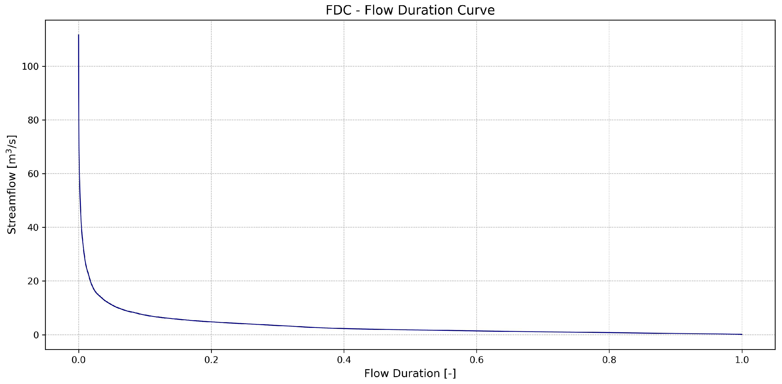
Figure 3 presents the flow duration of the Posina’s catchment, which permits the characterization of the natural hydrologic regime of the basin [27]. The hydrologic regime shows an erratic behavior, typical in a catchment where the mean interarrival between flow-producing rainfall events is larger than the typical duration of resulting flow pulses. A wider range of streamflows is observed between events, and the preferential state of the system is typically lower than the mean [28]. The Posina River may show no discharge in between summer rainfall events.

2.3. Experimental Setup

Before developing and training the models, we pre-processed the dataset to enhance its quality and eliminate inconsistencies or noise that could affect the accuracy of our models. First, we removed out-of-scale values using prior knowledge of the maximum and minimum hourly streamflow of the catchment area. Next, to address missing values, we applied linear interpolation for nearly all features, except for rain and temperature data, due to their nonlinear behavior. The physically based model, developed using HMS software, automatically handles missing sensor values by discarding them and interpolating them through inverse distance weighting (IDW) using data from other sensors. For the autoregressive and deep learning models, we imputed and pre-processed the temperature and rain-related missing data using the same method. This will allow us to give more importance to the sensors closer to the one presenting the missing value. We have fitted all the models using 70% of the dataset and tested the forecasting capabilities on the remaining 30 % except for the HEC-HMS model, where we have included as part of the fitting data also the flood event of October–November 2018 Figure 2b. In order to improve the stability of the LSTM model, we have scaled the data using Min–Max Normalization method. This transformation ensures that the minimum value of each feature becomes 0, the maximum value becomes 1, and all other values are scaled proportionally in between. To emulate the forecasting behavior of the other models with LSTM, we employed a rolling forecasting technique for streamflow prediction. This technique involves a sliding window to iteratively determine streamflow values. Importantly, the model’s predictions were used as input to forecast subsequent hours, allowing the model to capture the hydrological processes going on within the watershed, such as streamflow recessions corresponding to dry days. This approach in turn strongly reduces the LSTM model initial conditions importance, as the model quickly becomes independent by the initial observed values provided as it only uses predicted streamflow values after m prediction instances. A visual simplified explanation of this technique can be found in Figure 4, where (h) and m were set as an example to 6 for an easier visualization. By testing the LSTM model with the rolling window technique, we were able to compare the LSTM model with ARIMAX and the physically based model.

2.4. ARIMAX Model

The ARIMA model is a well-known autoregressive model used for time series forecasting in various contexts. In recent years, it has garnered significant attention in hydrological studies, as highlighted in the introduction Section 1. For this study, we used the extension of this model called ARIMAX, which enables the inclusion of exogenous variables. Models like ARIMAX rely on the assumption of stationarity of the time series under analysis. This does not imply that the series remains unchanged over time, but rather that the way it changes remains consistent over time. To ensure the suitability of ARIMAX modeling, we assessed the stationarity of the streamflow target time series for the Posina catchment using the augmented Dickey–Fuller (ADF) test [29]. The calculated p-value was 8.90 × 10 29 , confirming that the time series is stationary. The ARIMAX model relies on the following parameters: p, representing the autoregressive (AR) component or the number of lag observations in the model; d, denoting the degree of differencing required to achieve stationarity in the time series; and q corresponding to the size of the moving average (MA) window. Given that the streamflow time series passed the augmented Dickey–Fuller (ADF) test for stationarity, the parameter d was set to 0. To determine the values of parameters p and q, we analyzed the autocorrelation (ACF) and partial autocorrelation (PACF) plots to determine the optimal p, d, and q values. A parameter optimization analysis was conducted by comparing the Akaike Information Criterion (AIC) and the Bayesian Information Criterion (BIC) across different combinations of autoregressive (p) and moving average (q) orders. These metrics were used to evaluate the trade-off between model fit and complexity, supporting the selection of the most parsimonious ARIMAX configuration. The resulting evaluation scores are summarized in Table S3 of the Supplementary Materials. These values have also been refined by exploiting the automatic algorithm presented by Rob J. Hyndman and Yeasmin Khandakar in the work “Automatic Time Series Forecasting: The forecast Package for R” [30], which is a step-wise procedure traversing the space of models efficiently. The ARIMAX model parameters p, d, q have been set to 1, 0, 2, respectively. We have chosen to use the extended version of ARIMA, which allows for the inclusion of exogenous variables (the “X” in ARIMAX), we were able to incorporate rain and temperature forecasts as additional inputs for the streamflow predictions. Since ARIMAX is an autoregressive model, the forecasting of the streamflow involves employing a linear combination of past values of the streamflow along with any exogenous variables. The general ARIMAX equation is depicted in (1) where ϕ is the autoregressive term and p is the relative order. y t and y t i , are, respectively, the dependent variable value at time t and the lagged values of the dependent variable. θ is the moving average term with the relative order q. r represents the set of exogenous variables. X k t is the exogenous feature k at time t. β k and ϵ are, respectively, the strength coefficient of the exogenous variables and a random noise between the observed and predicted value.
y t = c + i = 1 p ϕ i y t i + j = 1 q θ j ϵ t j + k = 1 r β k X k t + ϵ t

2.5. Long Short-Term Memory (LSTM) Recurrent Neural Network

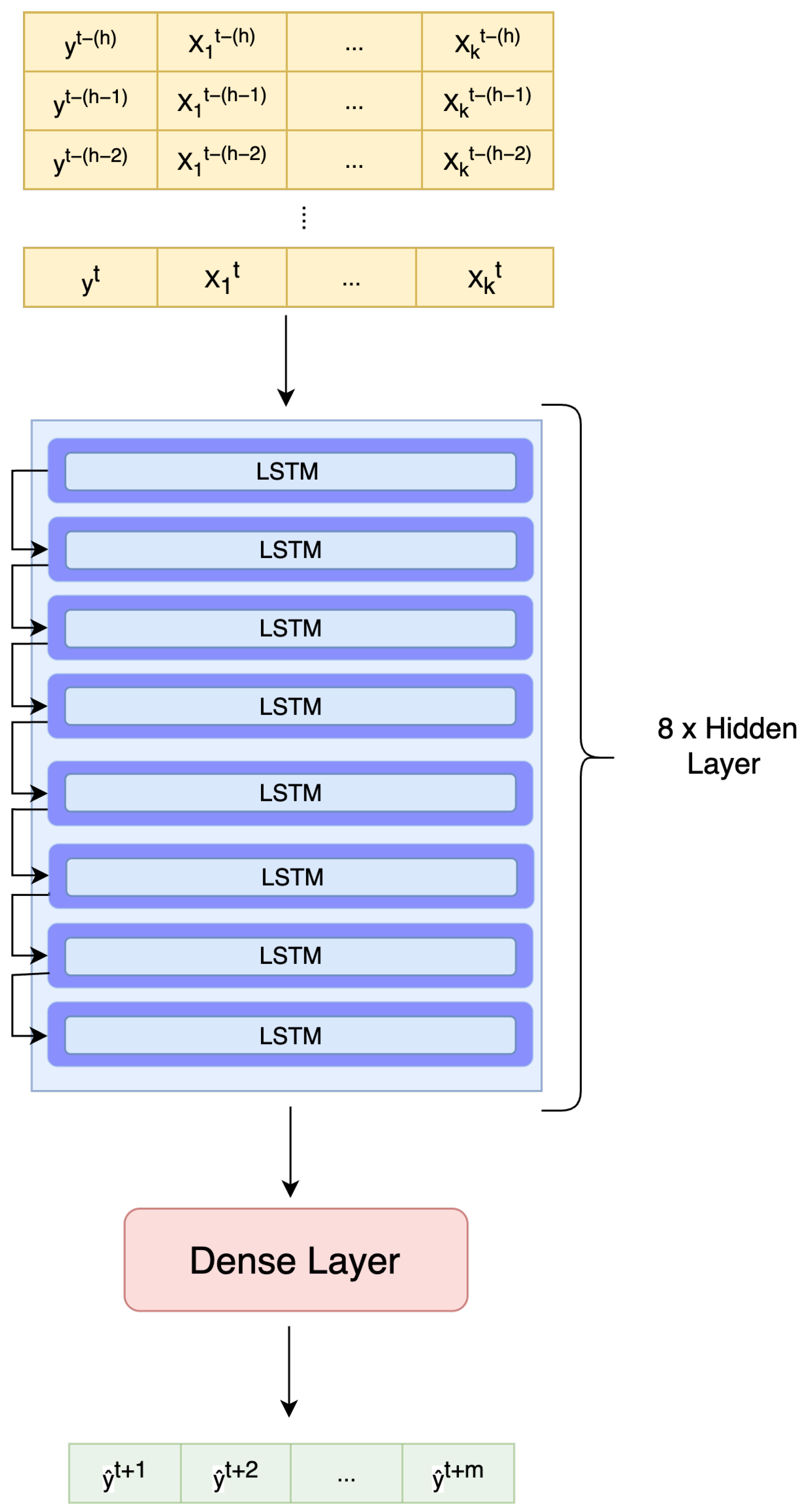
The Long Short-Term Memory (LSTM) model is a specific type of recurrent neural network (RNN) that has received a lot of interest in the hydrological field [16,21]. It has been presented by Hochreiter and Schmidhuber [31], to overcome the limitation of capturing and remembering long-term dependencies in sequential data. Before the training procedure, the constructed dataset was pre-processed to improve the efficiency and generalization of the model [32] as explained in the experimental setup section. Hyperparameter tuning plays a critical role in shaping the learning dynamics of the LSTM model and directly influences its forecasting performance. To identify an optimal configuration, we conducted a manual tuning procedure, systematically testing a range of hyperparameter combinations. The tuning process focused on the following key parameters: the model complexity (i.e., number of hidden layers and number of LSTM units per layer), batch size, initial learning rate, and the temporal structure of the input–output mapping, defined by the number of input hours (h) and predicted hours (m) at each inference step. The model consists of eight LSTM layers comprising 100 units each. A simplified representation of the model architecture is shown in Figure 5. The learning rate was initially set to 1 × 10 3 and dynamically adjusted during training to ensure adequate convergence and generalization. As a loss function, we employed the Mean Absolute Error (MAE) [33], presented in Equation (4), where n denotes the total number of instances, y i denotes the observed streamflow value, and y ^ i denotes the corresponding prediction. To prevent overfitting and improve generalization, an early stopping mechanism was implemented: if the validation loss did not improve for 25 consecutive epochs, the training process was halted and the model weights corresponding to the lowest validation loss were retained. Particular attention was given to exploring the effect of batch size and input sequence length (h). The sensitivity analysis was conducted to assess the impact of varying the batch size and number of input hours (h) on model training with a dynamically adjusted learning rate, and the results are reported in the Supplementary Materials. The resulting loss and learning rate curves for each configuration are shown in Figure S2, while the corresponding performance metrics are summarized in Table S4. Among the tested configurations, the final model was selected based on the best trade-off between training loss and validation loss, ensuring both the fit quality and generalization capability. A summary of the evaluated configurations and associated performance metrics is provided in the Supplementary Materials Table S4. The model was implemented using Python programming language, alongside the machine learning libraries Keras and TensorFlow. Each input to the trained model comprised all recorded streamflow, rainfall, and temperature values for the preceding h hours leading up to the inference instance. Additionally, the model incorporated the recorded hourly rainfall and temperatures for the next m hours forecast as for the exogenous values of the ARIMAX model. We assume that only the streamflow is recurrently predicted, whereas the weather data are the real ones (not predicted) at each time point. After tuning the parameters and hyperparameter tuning, the optimal values for h (previous hours) and m (number of forecast streamflow value at each instance) were determined to be 24, resulting in the model using the last 24 h of data to predict the subsequent 24 h.

2.6. Physically Based Model

Models presented in previous paragraphs were compared with a physically based model which was developed with the software Hydrologic Modelling System (HMS), version 6.11, by the US Army Corps of Engineers Hydrologic Engineering Center (HEC). HEC-HMS allows users to combine various procedures implemented to reproduce hydrological processes and build a customized hydrological model.
In the present application, the hydrological model was set to allow continuous simulations. This choice increases the complexity of the model as several additional processes must be considered than in event-based models, such as evapo-transpiration and soil moisture accounting, for example.
The spatial distribution of many variables influencing the runoff separation process implies the adoption of a spatial scale smaller than the entire watershed to account for such variability (e.g., elevation within the basin, land use, or soil type). The Posina river basin was thus discretized in 34 subcatchments (Figure S1 in Supplementary Materials) with an average size of 3.45 km2, within which spatial variables affecting hydrologic processes can be considered homogeneous. The number of subcatchments was not exaggerated to avoid excessive model complexity. In the proposed hydrological modeling, the soil moisture accounting model (hereinafter SMA) was adopted as it allows for describing the long-term dynamics of water content [34,35]. The SMA model represents the watershed with a series of interconnected storage layers. Current storage contents are calculated during the simulation and vary continuously both during dry or wet periods. Full details of this methodology can be found in the HEC-HMS Technical Reference Manual [36], from which a brief explanation was taken and described below. The different storage layers considered in this application are given as follows:
  • Canopy-interception storage represents the precipitation that is captured on trees, shrubs, and grasses, and does not reach the soil surface. Precipitation is the only inflow. Water in canopy interception storage is removed by evaporation;
  • Surface-interception storage is the volume of water held in shallow surface depressions. Inflows come from precipitation not captured by canopy interception and in excess of the infiltration rate. Outflows can be due to infiltration and to evapotranspiration (ET);
  • Soil-profile storage represents the water stored in the top layer of the soil. Inflow is infiltration from the surface. Outflows include percolation to a groundwater layer and ET. The soil profile is subdivided into two distinct layers. The upper zone is defined as the portion of the soil profile that will lose water to ET and/or percolation. The tension zone is defined as the area that will lose water to ET only. The upper zone represents the water held in the pores of the soil. The tension zone represents the water attached to soil particles. ET occurs from the upper zone first and tension zone last.
  • Groundwater storage layers in the SMA represent horizontal interflow processes. In this application, only one groundwater layer was used. Water percolates into groundwater storage layers from the soil profile. Losses from the groundwater storage layer are due to groundwater flow or to deep percolation. In the latter case, this water is considered lost from the system.
Details on the computation of flows between interconnected storage layers can be found in the HEC-HMS Technical Reference Manual [36].
Evapotranspiration was calculated at an hourly timescale through the Hargreaves method which also allow one to estimate the shortwave radiation from temperature data [37,38].
The hydrological model is completed with modules describing how the model transforms excess precipitation into runoff (transform process) and how the water content stored within the soil and groundwater layer becomes baseflow runoff (baseflow process).
The Transform process to route excess precipitation to the subcatchment outlet was described with the Clark Unit Hydrograph Model [36,39]. This method explicitly represents two critical processes in the transformation of excess precipitation to runoff: (1) the translation (or movement) of excess precipitation from its origin throughout the watershed to the outlet; and (2) the attenuation (or reduction) of the magnitude of the discharge as the excess precipitation is temporarily stored throughout the watershed.
The baseflow process is described by the Linear Reservoir Model, which uses one linear reservoir to simulate the recession of the baseflow after a storm event. According to the model, baseflow magnitude linearly depends on the amount of water stored within the groundwater layer of the SMA model. The linear release of water can be repeated in a waterfall process to increase the baseflow attenuation.
The methods described above provide a full description of the processes occurring at subcatchments which determine how rainfall forcing the system becomes discharges input within the river network. Flows are calculated at the subcatchment outlet and require an additional method to describe what occurs within the channels up to the catchment outlet. The Posina river has a typical mountainous behavior with steep and narrow channels, and as such, any attenuation process can be considered negligible. The methodology adopted for describing the routing process within the river network is the Lag Model, which simply considers that there is a translation of discharge within the river without any attenuation. Translation depends on the travel time within each river reach, which in turn mainly depends on the reach length and slope.
The hydrological model composed as described above requires the definition of several parameters for each subcatchment and river reach characterizing the Posina catchment. A list of the required parameters is provided below.
  • Canopy Interception
    -
    Canopy storage [mm], represents the maximum amount of water that can be held on leaves before through-fall to the surface begins.
  • Surface Interception
    -
    Surface storage [mm] represents the maximum amount of water that can be held on the soil surface before surface runoff begins.
  • Soil Moisture Accounting
    -
    Soil storage [mm], total storage available in the soil layer;
    -
    Tension storage [mm], amount of soil storage that is not drained by percolation but only by evapotranspiration;
    -
    Groundwater storage [mm] represents the total storage in the groundwater layer;
    -
    Impervious percentage [%], percentage of the subcatchment with direct runoff production (no infiltration);
    -
    Maximum infiltration rate [mm/h] sets the upper bound on infiltration from the surface storage into the soil;
    -
    Soil percolation [mm/h] sets the upper bound on percolation from the soil storage into the groundwater;
    -
    Groundwater percolation rate [mm/h] sets the upper bound on deep percolation.
  • Clark Unit Hydrograph
    -
    Time of concentration [h] defines the maximum response time in the sub-basin;
    -
    Storage coefficient [h], accounts for storage effects within the subcatchment surface.
  • Linear Reservoir Baseflow
    -
    Groundwater coefficient [h] is used as the time lag on a linear reservoir for transforming water in storage to become lateral outflow;
    -
    Number of steps [−], which increases the attenuation of baseflow (minimum attenuation with a single step; attenuation increases as the reservoir release is repeated several times).
  • Reach Routing
    -
    Lag [min], time that the inflow hydrograph will be translated.
All parameters listed above were estimated depending on information available at the Posina catchment (soil atlas, soil use) and on the physical features of each element of the river system (reach length, slope and width). Some of these were determined thanks to empirical formulation (time of concentration), while others were obtained by the calibration of the model against observed flows. The model parameters have been calibrated on the same training period of the other models. A single set of parameters was thus adapted. The calibration process focused on a limited set of parameters. Specifically, canopy and surface storage values were calibrated uniformly across the basin within plausible ranges (0–30 mm and 0–50 mm, respectively), reflecting the catchment’s forested land cover. The runoff response was shaped by calibrating the storage and groundwater coefficients of the Clark unit hydrograph and baseflow modules, expressed as multipliers of the time of concentration (Tc). The final values, 16×Tc and 170×Tc, respectively, were selected after iterative tuning to match the observed flood dynamics.
The model also requires initial conditions which, however, have had negligible impact on the model performance, as in long-term continuous simulations, the initial error is forgotten by the system after a rainfall determining soil saturation.

2.7. Performance Evaluation Criteria

All predictions generated by the models have been evaluated and compared using multiple performance criteria. We utilized two well-known metrics widely applied in the hydrological field: the Nash–Sutcliffe Efficiency index (NSE) and the Kling–Gupta Efficiency index (KGE). Additionally, we measured the previously presented mean absolute error (MAE) from Equation (4), not only as a loss function for optimization, but also as an evaluation criterion. To measure MAE, we have exploited the method implemented into the scikit-learn Python library [40]. To compute NSE and and KGE, we have used the hydroeval open source Python library [41].

2.7.1. Nash–Sutcliffe Efficiency Index (NSE)

The Nash–Sutcliffe efficiency index is a widely used and reliable statistic for assessing the goodness-of-fit of hydrologic models. One of its main advantage is that it can be applied to a variety of model types [42].
In Equation (2), y t is the observed value at time t, y ^ t is the predicted value at the same time t, y t ¯ is the mean of the observed values, and n refers to the total number of observation. The NSE value ranges from to 1, where 1 signifies a perfect model with an estimation error variance from the original measurements equal to zero. An NSE value equal to 0 indicates that the model under investigation incorporates the same predictive capabilities as the mean of the forecast time series. Higher NSE values are associated with greater predictive capabilities.
NSE = 1 t = 1 n ( y t y ^ t ) 2 t = 1 n ( y t y ¯ ) 2

2.7.2. Kling–Gupta Efficiency Index (KGE)

The Kling–Gupta efficiency index (KGE) [43] was introduced as an improvement over the NSE, in order to capture an additional aspect of the model such as correlation, bias, and variability. The term r in Equation (3) represent the Pearson correlation coefficient between observed and simulated values. α is the measure of the flow variability error calculated as the ratio between the variance of the simulated time series and the variance of the observed time series. β is the ratio of the mean of the simulated values to the mean of the observed values, also identified as the bias term. Analogous to NSE, KGE = 1 indicates perfect agreement between simulations and observations while KGE = 0 or KGE < 0 indicates that the mean of observations provides better estimates than simulations [44,45].
KGE = 1 ( r 1 ) 2 + ( α 1 ) 2 + ( β 1 ) 2

2.7.3. Mean Absolute Error (MAE)

The mean absolute error (MAE) described by the Formula (4). The main difference of measuring the predictive capabilities of a model with MAE instead of using NSE or KGE, providing a straightforward measure of the absolute accuracy of the model’s predictions [20]. The optimal MAE value is 0, indicating perfect prediction accuracy. Higher values of this index are associated with worse forecasting capabilities.
Since we are computing the absolute difference between the observed and the predicted value, the MAE unit measure is the average (AVG) m3/s measure at each hour.
MAE = 1 n t = 1 n y t y ^ t

3. Results

We evaluated the forecasting performance of all models over the entire testing set by computing the metrics previously described, namely NSE, KGE, and MAE. These metrics were used to assess each model’s predictive accuracy on unseen testing data, and the corresponding results are summarized in Table 1. To provide a visual comparison, we present plots showing predicted versus observed streamflow values. Each plot reports time on the x axis (in dates) and streamflow on the y axis, expressed in average m3/s. In addition to the standard linear scale, we also include plots using the symlog (symmetric logarithmic) scale on the y axis. This scale is particularly useful for representing data that spans several orders of magnitude while retaining sensitivity to low-flow conditions, including near-zero and negative values, without distortion.

3.1. ARIMAX Forecasting Results

The images in Figure 6a,b depict the forecasting results of the ARIMAX model on the testing dataset, using the autoregressive principle discussed in the preceding section. The green line refers to the real observed values, while the red line refers to the predicted simulated values from the model.
Measured values of NSE, MSE, and MAE has been collected in Table 1. The NSE stands at 0.67, indicating that the model’s estimation error variance is lower compared to the variance derived from the mean observed data. However, the KGE value hovers around 0.50 highlighting the imperfect correlation between the observed and predicted values. The average magnitude of errors between predicted and actual values, as measured by the mean absolute error, is 1.16 m3/s.
Figure 6. (a) ARIMAX testing set hourly forecasting. In red, the predicted values from the ARIMAX model, and in green, the original observed values for the same period. (b) ARIMAX testing set hourly forecasting. y axis symlog scaled. The y axis is scaled using the symlog (symmetric log) scale method.
Water 17 02341 g006

3.2. LSTM Forecasting Results

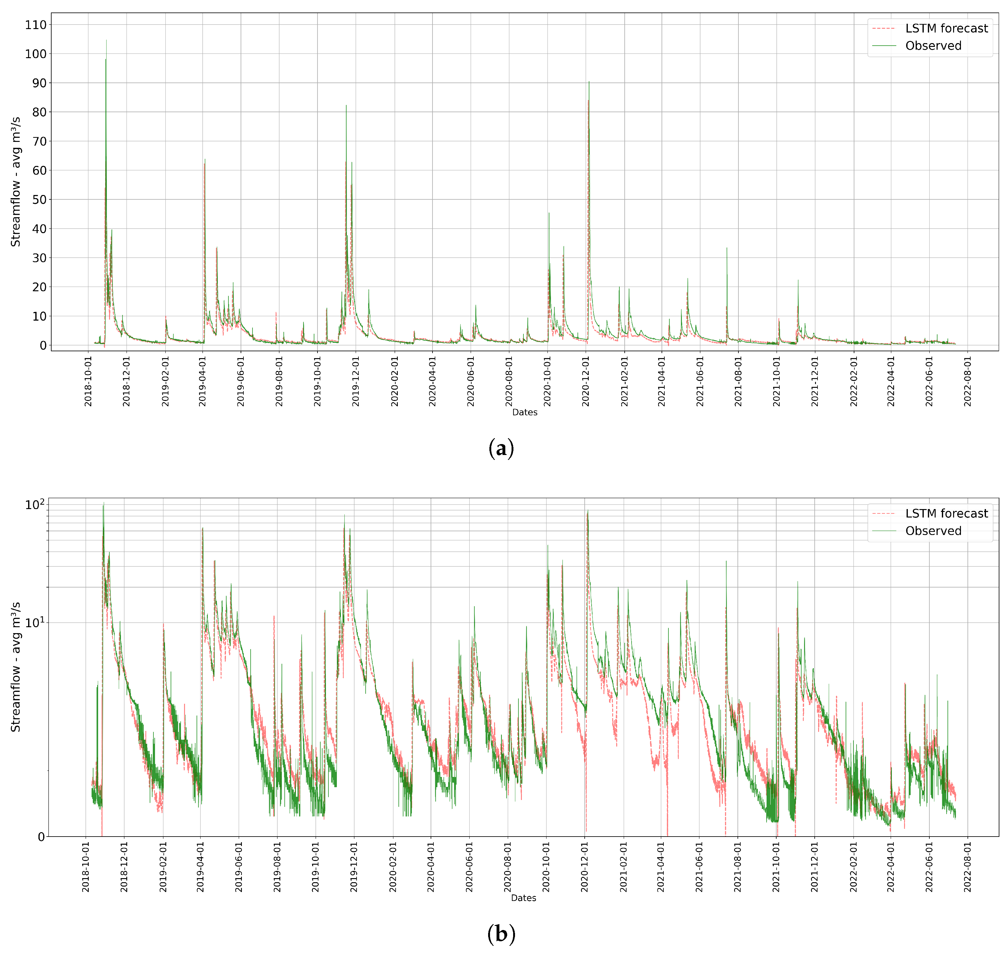
As mentioned earlier, we assessed the predictions produced by our rolling forecasting LSTM model. To do this, we reconstructed the entire testing set by forecasting the next 24 h, advancing one hour at a time in the inference process. We retained only the value forecast for the next hour (t + 1) to reconstruct the entire testing set. At each step, we discarded the forecast values from t + 2 to t + 48. In this way, the model quickly became independent from the initial condition, relying on its own predictions to forecast the subsequent values. For simplicity, the color of the observed and predicted values are again green and red, respectively.
The evaluation metrics values presented in Table 1 reveal that the LSTM model demonstrates proficient predictive capability for the overall testing set, with NSE, KGE, and MAE values of 0.93, 0.82, and 0.75, respectively.
Figure 7. (a) LSTM testing set rolling forecasting. The red line depicts the predicted values of the LSTM model, while the green line represents the original observed values. (b) LSTM testing set rolling forecasting, y axis symlog scaled. The y axis is scaled using the symlog (symmetric log) scale method.
Water 17 02341 g007

3.3. Physically Based Model Forecasting Results
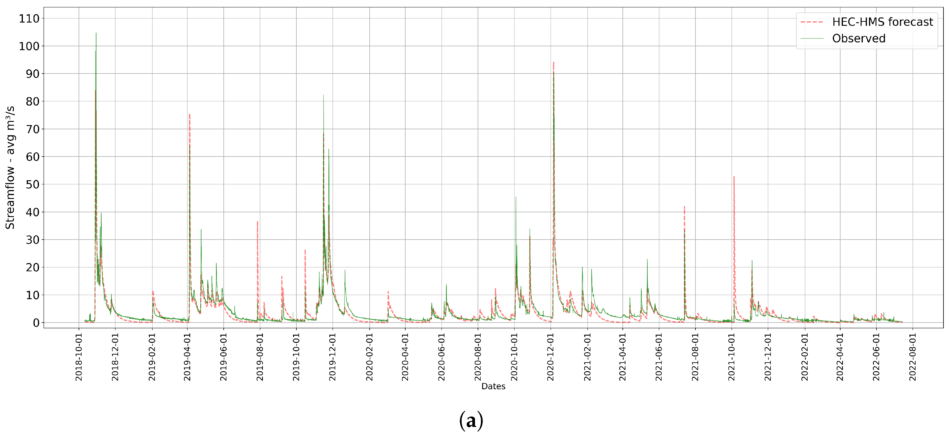
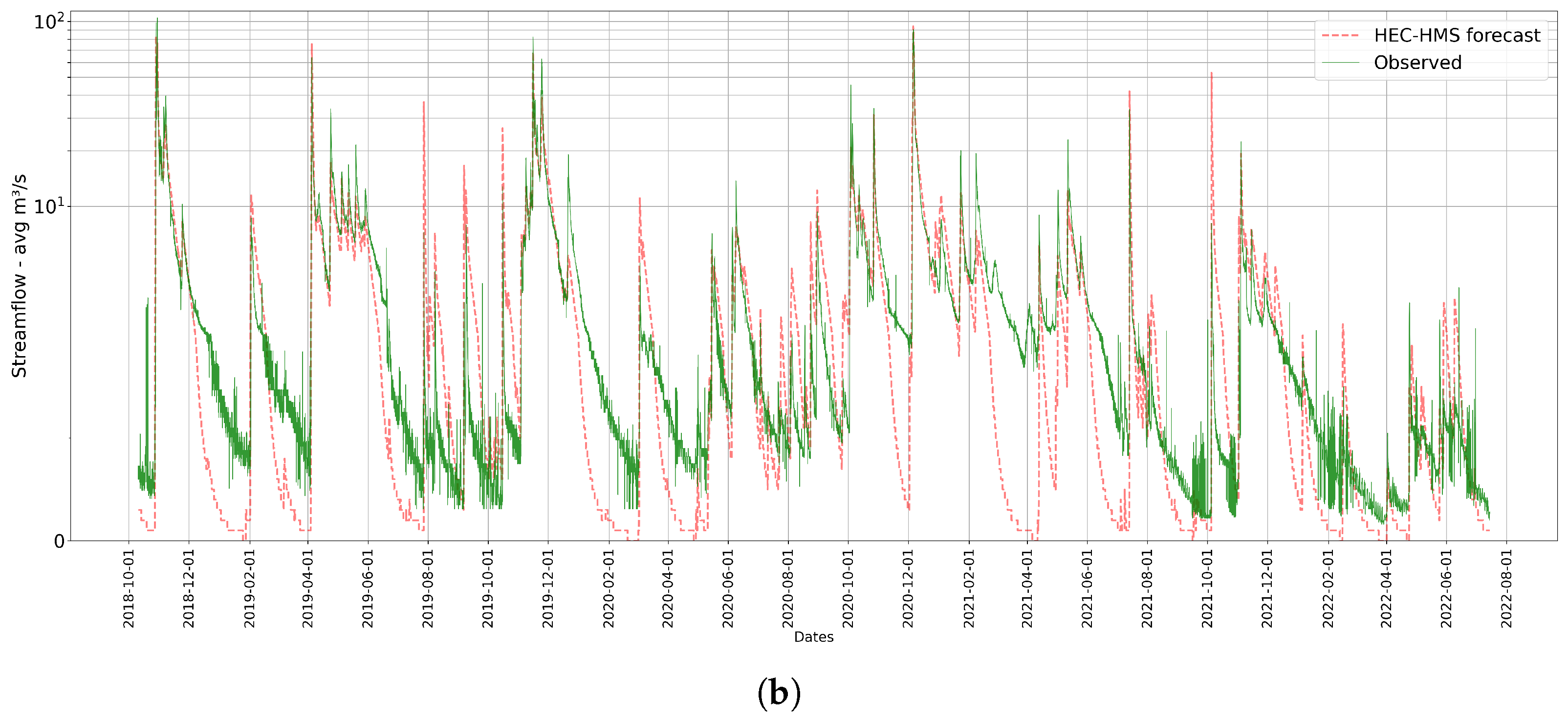
For the same period of testing, we evaluated the prediction capability of the traditional physically based hydrological model. As for the previous images, the green line refers to the original observed values, while the red line refers to the predicted values from the model.
Figure 8. (a) HEC-HMS physically based model prediction on testing set. The red line depicts the predicted values from the physically based model, while the green line shows the original observed values. (b) HEC-HMS physically based model prediction on testing set. y axis symlog scaled. The red line depicts the predicted values from the physically based model, and the green line represents the original observed values.
Water 17 02341 g008aWater 17 02341 g008b
From Table 1, we can see that the physically based model achieved NSE, KGE, and MAE values of 0.82, 0.85, and 1.27, respectively.

3.4. Models Performance During Significant Flood Events

To gain deeper insights into the performance of different models, we investigate their streamflow forecasting capabilities during significant flood events. Specifically, we examine three distinct streamflow conditions available in our dataset, focusing on two significant flood events from 2010 and 2018 and one occasional summer rain event that occurred in July 2021. We selected these three events because they represent a diverse range of hydrological conditions, major floods and a more typical rainfall event, allowing us to test the models’ robustness across different scenarios. This diverse selection helps to ensure a comprehensive evaluation of model capabilities under varying streamflow patterns. In all the images, we represent the streamflow observed values in green, while the red, purple, and yellow refer to the LSTM, ARIMAX, and physically based models forecast values, respectively.

3.4.1. Model Comparison Flood Event October–November 2018
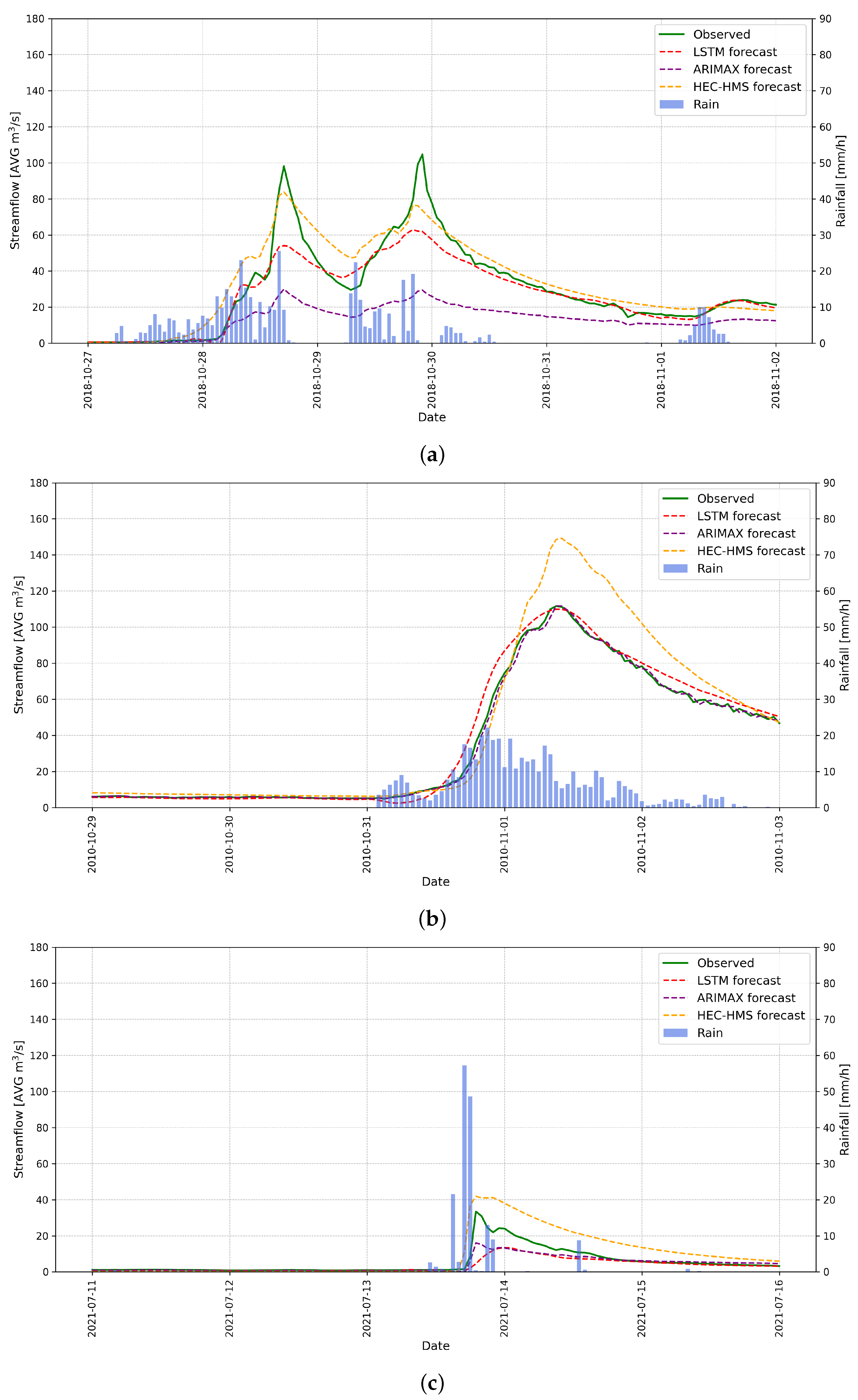
The image in Figure 9a depicts the prediction capabilities of the flood event occurs within the validation set of our dataset, specifically between October and November of 2018, of the three models. The ARIMAX and LSTM models were not trained on this particular event, whereas the traditional physically based model included this event as part of its fitting data. During the flood event, two main streamflow peaks were observed. The first peak occurred on October 28th around 16:00, reaching approximately 100 AVG m3/s, while the second peak was recorded on October 29th at approximately 22:00, with a maximum value close to 105 AVG m3/s. Both ARIMAX and LSTM models showed an underestimation of the observed values. The LSTM model predicted the two peaks with values of approximately 55 AVG m3/s and 62 AVG m3/s, respectively. ARIMAX estimated both peaks at approximately 30 AVG m3/s. The HEC-HMS physically based model estimated the peaks at approximately 85 AVG m3/s and 78 AVG m3/s, respectively, which were closer in magnitude to the observed values. All models showed a generally coherent timing of the peak occurrences, with minimal time shifts relative to the observed values.
Figure 9. Model performance comparison for (a) October–November 2018 flood event. (b) October–November 2010 flood event. (c) Occasional summer rain event of July 2021.
Water 17 02341 g009

3.4.2. Model Comparison Flood Event October–November 2010

Figure 9b illustrates the 3 different model estimations of the October–November 2010 flood event, which is part of the training set. Including this event in the comparison serves to highlight the behavior of the models on data also used during training or calibration. This provides useful insights into their predictive tendencies, such as overfitting or smoothing. During the 2010 flood event, a single pronounced streamflow peak was observed on November 1st around 02:00, reaching approximately 110 AVG m3/s. The LSTM and ARIMAX models predict peak values very close to the observed data, with estimated maxima of approximately 108 AVG m3/s and 110 AVG m3/s, respectively. However, while ARIMAX reproduces the signal with high accuracy due to having been fit on these data, the LSTM model yields a smoother predictive curve. In contrast, the HEC-HMS physically based model significantly overestimated the peak, with a value around 150 AVG m3/s, and exhibited a slower recession phase compared to both the observed data and the other models.

3.4.3. Model Comparison Occasional Rain Event July 2021

Figure 9c shows the performance of the three models during the isolated summer rainfall event of 2021. In this case, the streamflow response exhibited a very sharp rise compared to the other events, with the observed peak reaching approximately 35 AVG m3/s. The HEC-HMS model overestimated the peak with a predicted value of about 42 AVG m3/s, and showed a slower recession phase relative to the observed streamflow. Both LSTM and ARIMAX models underestimated the peak, with predicted values below 20 AVG m3/s. The LSTM model, in particular, produced a smoother streamflow response compared to the observed rapid dynamics.

4. Discussion and Conclusions

In this study, we have compared three different approaches for streamflow forecasting in a challenging Italian natural catchment, characterized by multiple types of soils, intense rainfall periods, and strong seasonal variability. The LSTM and traditional physically based hydrological models have remarkably better capabilities on streamflow forecasting compared to the ARIMAX autoregressive model. Inspecting the images depicted in Figure 6 and reported metrics in Table 1. It is possible to notice that the autoregressive ARIMAX model is capable of catching the overall streamflow trend with sufficient correctness to detect the different streamflow scenarios. However, it struggles with accurately predicting abrupt changes in streamflow, underestimating peaks, and introducing noise over time due to autoregressive prediction behavior. Furthermore, the model introduces noticeable noise in regions near zero streamflow values, and as time progresses, the model seems to accumulate errors, leading to a degradation in prediction accuracy over time. Its performance is significantly lower compared to the LSTM and physically based models in capturing peak values and the dynamics of rapid increases. Being simple to implement due to the low computational cost and the well-known multiple programming libraries available for development, it can be used as a baseline approach to study the attitude of the streamflow under investigation. The LSTM model exhibits excellent performance, as evidenced by the metrics reported in Table 1. NSE and KGE values of 0.93 and 0.82, respectively, highlight the model’s strength in capturing the correlation between observed and predicted values, indicating good agreement in the temporal pattern of the data. Compared to the estimation of the ARIMAX model (Figure 6), LSTM introduces significantly less noise near zero-flow values, as illustrated in Figure 7a,b. Furthermore, the LSTM model operates in a rolling forecast mode, where predicted values are fed back as input for subsequent time steps. This recursive prediction strategy demonstrates the model’s ability to generalize and maintain stability over time, effectively capturing the overall trend of the testing set without external correction. Specifically, it effectively manages most streamflow peaks, even in instances where extreme cases were absent from the training data. The LSTM model shows optimal capabilities in capturing both peak flows and their subsequent recession phases compared to the physically based and ARIMAX models (Figure 6b and Figure 8b). This highlights its enhanced ability to handle rapid hydrological responses typical of fast-responding catchments, delivering sharper and more stable predictions during high-flow conditions. While the training process of the LSTM model can be relatively time-consuming and requires careful parameter and hyperparameter tuning, its overall computational demand remains considerably lower than that of setting up and calibrating a full physically based model. The LSTM model tends to smooth out slightly rapid streamflow changes, but the model’s performance is commendable for streamflow prediction, especially when sufficient training data are available. The physically based model relies on the physical natural behaviors of the catchment which permits an efficient ability to determine the overall streamflow trend, pikes, and rare events that even the other data-driven model may struggle to detect. Despite this, the model shows a tendency to overestimate peak values and often exhibited a rapid decline after peak events, missing the smooth recession observed in actual data (Figure 8b). While the physically based model benefits from its physical basis and ability to incorporate various hydrological processes, it requires careful calibration and may not always generalize well to all events observed within the training and testing sets. These behaviors are also reflected in the analysis of the three representative flood events illustrated in Figure 9. In the 2010 flood event (Figure 9b), all models captured the peak timing consistently, with the LSTM and ARIMAX models predicting peak values close to the observed 110 AVG m3/s. However, the HEC-HMS model significantly overestimated the peak and showed a slower post-peak recession. A similar overestimation by the physically based model is observed during the occasional summer rainfall event of July 2021 (Figure 9c). The particularly high accuracy of the ARIMAX model in this case can be attributed to the fact that this flood event is included in the training set, allowing the model to directly fit the observed dynamics. In contrast, although the LSTM model was also trained on the same period and demonstrates good performance, it employs a rolling forecasting strategy, where its own previous outputs are iteratively used as inputs for subsequent predictions. This approach introduces a degree of compounding uncertainty, which tends to smooth the resulting predictions. In the 2018 flood event (Figure 9a), HEC-HMS produced peak estimates closer to the observed values, although with smoother transitions. This behavior is likely due to the incorporation of physical knowledge calibrated for the basin, combined with the fact that the event data were part of the model’s calibration set. As discussed in the Results section, both the LSTM and ARIMAX models underestimate peak values in certain cases, likely due to their reliance on previously observed data, which results in smoother predictions and reduced sensitivity to sudden flow changes. However, the LSTM model consistently provides more accurate and homogeneous streamflow predictions compared to the ARIMAX model. It has also demonstrated a remarkable ability to handle different hydrological conditions, often achieving performances comparable to, or even exceeding, those of the physically based model. Being trained specifically on the basin under examination, the LSTM model effectively leverages the rolling forecasting approach, using its own predictions iteratively as inputs for future time steps. This characteristic enables the model to maintain high predictive performance over extended forecast horizons. Furthermore, its adaptive nature and reduced need for complex parametrization make it a practical and efficient alternative for real-world streamflow forecasting applications, especially when compared to the more resource-intensive setup and calibration required by traditional physically based models. Despite the promising results achieved, several limitations must be acknowledged. The LSTM model, implemented with a rolling forecasting strategy, is well suited to adapt when trained on a single basin; however, this study focuses on a single catchment with specific hydrological and geomorphological characteristics, which may limit the generalizability of the findings. The Posina basin is a fast-responding alpine catchment characterized by intense rainfall and strong seasonality, and the trained models may have implicitly learned behaviors unique to this context. As a result, further validation across multiple catchments with diverse hydrological regimes is essential to assess the robustness and transferability of the proposed approaches. Additionally, while the LSTM model demonstrated excellent predictive performance, it remains highly dependent on the availability and quality of historical data. Limited data length, or shifts in climate or land use, could impact the model’s effectiveness in real-world applications. Future work will explore the impact of limited data availability and the development of hybrid modeling approaches that integrate the strengths of data-driven and physically based paradigms. Embedding physical constraints or process-based layers within deep learning architectures may improve model interpretability, reduce calibration requirements, and enhance generalization to ungauged or poorly instrumented basins.

Supplementary Materials

The following supporting information can be downloaded at https://www.mdpi.com/article/10.3390/w17152341/s1, Figure S1: Posina river subcatchments. Figure S2: Sensitivity analysis of the LSTM model across batch sizes and input sequence lengths. Table S1: Subbasin parameters. Table S2: River reach parameters. Table S3: ARIMAX sensitivity analysis AIC and BIC. Table S4: LSTM hyperparameter tuning: batch size and input length.

Author Contributions

Conceptualization, D.P., G.L., A.F., P.F. and E.G.; methodology, D.P. and G.L.; software, D.P. and G.L.; validation, D.P., G.L. and E.G.; formal analysis, D.P.; investigation, D.P. and G.L.; resources, D.P.; data curation, D.P., P.F. and E.G.; writing, original draft preparation, D.P.; writing, review and editing, G.L., P.F. and E.G.; visualization, D.P., G.L. and E.G.; supervision, D.P., G.L., A.F., P.F. and E.G.; project administration, D.P. All authors have read and agreed to the published version of the manuscript.

Funding

This research has been supported from PNRR DM352: 38-033-19-DOTT1433495-2235.

Data Availability Statement

As mentioned in the text, meteorological and discharge stations within and nearby the catchment are administered by the Environmental Protection Agency, that makes those data available without any limits of elaboration usage and distribution.

Conflicts of Interest

Authors Diego Perazzolo, Gianluca Lazzaro, Alvise Fiume and Pietro Fanton were employed by the company I4 Consulting S.R.L. The remaining authors declare that the research was conducted in the absence of any commercial or financial relationships that could be construed as a potential conflict of interest.

Abbreviations

The following abbreviations are used in this manuscript:
LSTMLong Short-Term Memory
ARIMAXAutoregressive Integrated Moving Average with Exogenous inputs
RNNRecurrent Neural Network
HEC-HMSHydrologic Engineering Center-Hydrologic Modeling System
NSENash–Sutcliffe Efficiency
KGEKling–Gupta Efficiency
MAEMean Absolute Error
IDFIntensity–Duration–Frequency
SMASoil Moisture Accounting
ETEvapotranspiration
AVGAverage
ADFAugmented Dickey–Fuller
IDWInverse Distance Weighting
FDCFlow Duration Curve

References

  1. Blöschl, G. Predictions in ungauged basins—Where do we stand? Proc. Int. Assoc. Hydrol. Sci. 2016, 373, 57–60. [Google Scholar] [CrossRef]
  2. Troin, M.; Arsenault, R.; Wood, A.W.; Brissette, F.; Martel, J.L. Generating ensemble streamflow forecasts: A review of methods and approaches over the past 40 years. Water Resour. Res. 2021, 57, e2020WR028392. [Google Scholar] [CrossRef]
  3. Devia, G.K.; Ganasri, B.P.; Dwarakish, G.S. A review on hydrological models. Aquat. Procedia 2015, 4, 1001–1007. [Google Scholar] [CrossRef]
  4. Freeze, R.A.; Harlan, R. Blueprint for a physically-based, digitally-simulated hydrologic response model. J. Hydrol. 1969, 9, 237–258. [Google Scholar] [CrossRef]
  5. Kirchner, J.W. Getting the right answers for the right reasons: Linking measurements, analyses, and models to advance the science of hydrology. Water Resour. Res. 2006, 42, W03S04. [Google Scholar] [CrossRef]
  6. Chow, V.T.; Maidment, D.R.; Mays, L.W. Applied Hydrology; McGraw-Hill: New York, NY, USA, 1988. [Google Scholar]
  7. Wood, E.F.; Roundy, J.K.; Troy, T.J.; Van Beek, L.; Bierkens, M.F.; Blyth, E.; de Roo, A.; Döll, P.; Ek, M.; Famiglietti, J.; et al. Hyperresolution global land surface modeling: Meeting a grand challenge for monitoring Earth’s terrestrial water. Water Resour. Res. 2011, 47, 5. [Google Scholar] [CrossRef]
  8. Kratzert, F.; Klotz, D.; Brenner, C.; Schulz, K.; Herrnegger, M. Rainfall–runoff modelling using long short-term memory (LSTM) networks. Hydrol. Earth Syst. Sci. 2018, 22, 6005–6022. [Google Scholar] [CrossRef]
  9. Dorigo, W.; Wagner, W.; Albergel, C.; Albrecht, F.; Balsamo, G.; Brocca, L.; Chung, D.; Ertl, M.; Forkel, M.; Gruber, A.; et al. ESA CCI Soil Moisture for improved Earth system understanding: State-of-the art and future directions. Remote Sens. Environ. 2017, 203, 185–215. [Google Scholar] [CrossRef]
  10. Ochsner, T.E.; Cosh, M.H.; Cuenca, R.H.; Dorigo, W.A.; Draper, C.S.; Hagimoto, Y.; Kerr, Y.H.; Larson, K.M.; Njoku, E.G.; Small, E.E.; et al. State of the art in large-scale soil moisture monitoring. Soil Sci. Soc. Am. J. 2013, 77, 1888–1919. [Google Scholar] [CrossRef]
  11. Teng, J.; Jakeman, A.J.; Vaze, J.; Croke, B.F.; Dutta, D.; Kim, S. Flood inundation modelling: A review of methods, recent advances and uncertainty analysis. Environ. Model. Softw. 2017, 90, 201–216. [Google Scholar] [CrossRef]
  12. Gupta, H.V.; Sorooshian, S.; Yapo, P.O. Status of automatic calibration for hydrologic models: Comparison with multilevel expert calibration. J. Hydrol. Eng. 1999, 4, 135–143. [Google Scholar] [CrossRef]
  13. Beven, K.J. Rainfall-Runoff Modelling: The Primer; John Wiley & Sons: Hoboken, NJ, USA, 2012. [Google Scholar]
  14. Kaur, J.; Parmar, K.S.; Singh, S. Autoregressive models in environmental forecasting time series: A theoretical and application review. Environ. Sci. Pollut. Res. 2023, 30, 19617–19641. [Google Scholar] [CrossRef]
  15. Dimri, T.; Ahmad, S.; Sharif, M. Time series analysis of climate variables using seasonal ARIMA approach. J. Earth Syst. Sci. 2020, 129, 1–16. [Google Scholar] [CrossRef]
  16. Benvenuto, D.; Giovanetti, M.; Vassallo, L.; Angeletti, S.; Ciccozzi, M. Application of the ARIMA model on the COVID-2019 epidemic dataset. Data Brief 2020, 29, 105340. [Google Scholar] [CrossRef]
  17. Myronidis, D.; Ioannou, K.; Fotakis, D.; Dörflinger, G. Streamflow and hydrological drought trend analysis and forecasting in Cyprus. Water Resour. Manag. 2018, 32, 1759–1776. [Google Scholar] [CrossRef]
  18. Moura, R.; Mendes, A.; Cascalho, J.; Mendes, S.; Melo, R.; Barcelos, E. Predicting Flood Events with Streaming Data: A Preliminary Approach with GRU and ARIMA. In Proceedings of the International Conference on Optimization, Learning Algorithms and Applications, Tenerife, Spain, 24–26 July 2024; Springer: Berlin/Heidelberg, Germany, 2024; pp. 319–332. [Google Scholar]
  19. Hewamalage, H.; Bergmeir, C.; Bandara, K. Recurrent neural networks for time series forecasting: Current status and future directions. Int. J. Forecast. 2021, 37, 388–427. [Google Scholar] [CrossRef]
  20. Sabzipour, B.; Arsenault, R.; Troin, M.; Martel, J.L.; Brissette, F.; Brunet, F.; Mai, J. Comparing a long short-term memory (LSTM) neural network with a physically-based hydrological model for streamflow forecasting over a Canadian catchment. J. Hydrol. 2023, 627, 130380. [Google Scholar] [CrossRef]
  21. Ayzel, G.; Heistermann, M. The effect of calibration data length on the performance of a conceptual hydrological model versus LSTM and GRU: A case study for six basins from the CAMELS dataset. Comput. Geosci. 2021, 149, 104708. [Google Scholar] [CrossRef]
  22. Khatun, A.; Chatterjee, C.; Sahu, G.; Sahoo, B. A novel smoothing-based long short-term memory framework for short-to medium-range flood forecasting. Hydrol. Sci. J. 2023, 68, 488–506. [Google Scholar] [CrossRef]
  23. Hu, Y.; Huber, A.; Anumula, J.; Liu, S.C. Overcoming the vanishing gradient problem in plain recurrent networks. arXiv 2018, arXiv:1801.06105. [Google Scholar]
  24. Kratzert, F.; Gauch, M.; Klotz, D.; Nearing, G. HESS Opinions: Never train a Long Short-Term Memory (LSTM) network on a single basin. Hydrol. Earth Syst. Sci. 2024, 28, 4187–4201. [Google Scholar] [CrossRef]
  25. Leščešen, I.; Tanhapour, M.; Pekárová, P.; Miklánek, P.; Bajtek, Z. Long Short-Term Memory (LSTM) Networks for Accurate River Flow Forecasting: A Case Study on the Morava River Basin (Serbia). Water 2025, 17, 907. [Google Scholar] [CrossRef]
  26. De la Fuente, L.A.; Ehsani, M.R.; Gupta, H.V.; Condon, L.E. Toward interpretable LSTM-based modeling of hydrological systems. Hydrol. Earth Syst. Sci. 2024, 28, 945–971. [Google Scholar] [CrossRef]
  27. Lazzaro, G.; Basso, S.; Schirmer, M.; Botter, G. Water management strategies for run-of-river power plants: Profitability and hydrologic impact between the intake and the outflow. Water Resour. Res. 2013, 49, 8285–8298. [Google Scholar] [CrossRef]
  28. Botter, G.; Basso, S.; Rodriguez-Iturbe, I.; Rinaldo, A. Resilience of river flow regimes. Proc. Natl. Acad. Sci. USA 2013, 110, 12925–12930. [Google Scholar] [CrossRef] [PubMed]
  29. Paparoditis, E.; Politis, D.N. The asymptotic size and power of the augmented Dickey–Fuller test for a unit root. Econom. Rev. 2018, 37, 955–973. [Google Scholar] [CrossRef]
  30. Hyndman, R.J.; Khandakar, Y. Automatic time series forecasting: The forecast package for R. J. Stat. Softw. 2008, 27, 1–22. [Google Scholar] [CrossRef]
  31. Hochreiter, S.; Schmidhuber, J. Long short-term memory. Neural Comput. 1997, 9, 1735–1780. [Google Scholar] [CrossRef]
  32. Ali, P.J.M.; Faraj, R.H.; Koya, E.; Ali, P.J.M.; Faraj, R.H. Data normalization and standardization: A technical report. Mach. Learn. Sci. Technol. 2014, 1, 1–6. [Google Scholar]
  33. Botchkarev, A. Performance metrics (error measures) in machine learning regression, forecasting and prognostics: Properties and typology. arXiv 2018, arXiv:1809.03006. [Google Scholar]
  34. Leavesley, G.H. Precipitation-Runoff Modeling System: User’s Manual; US Department of the Interior: Burlington, MA, USA, 1984; Volume 83.
  35. Bennett, T.H. Development and Application of a Continuous Soil Moisture Accounting Algorithm for the Hydrologic Engineering Center Hydrologic Modeling System (HEC-HMS). Master’s Thesis, University of California, Davis, CA, USA, 1998. [Google Scholar]
  36. U.S. Army Corps of Engineers. Hydrologic Modeling System HEC-HMS Technical Reference Manual; Hydrologic Engineering Center: Davis, CA, USA, 2000. [Google Scholar]
  37. Hargreaves, G.H.; Allen, R.G. History and evaluation of Hargreaves evapotranspiration equation. J. Irrig. Drain. Eng. 2003, 129, 53–63. [Google Scholar] [CrossRef]
  38. Hargreaves, G.H.; Samani, Z.A. Reference crop evapotranspiration from temperature. Appl. Eng. Agric. 1985, 1, 96–99. [Google Scholar] [CrossRef]
  39. Clark, C. Storage and the unit hydrograph. Trans. Am. Soc. Civ. Eng. 1945, 110, 1419–1446. [Google Scholar] [CrossRef]
  40. Kramer, O. Scikit-learn. In Machine Learning for Evolution Strategies; Springer: Berlin/Heidelberg, Germany, 2016; pp. 45–53. [Google Scholar]
  41. Hallouin, T. Hydroeval: An Evaluator for Streamflow Time Series in Python. 2021. Available online: https://pypi.org/project/hydroeval/0.0.1.post1/ (accessed on 10 February 2024).
  42. McCuen, R.H.; Knight, Z.; Cutter, A.G. Evaluation of the Nash–Sutcliffe efficiency index. J. Hydrol. Eng. 2006, 11, 597–602. [Google Scholar] [CrossRef]
  43. Gupta, H.V.; Kling, H.; Yilmaz, K.K.; Martinez, G.F. Decomposition of the mean squared error and NSE performance criteria: Implications for improving hydrological modelling. J. Hydrol. 2009, 377, 80–91. [Google Scholar] [CrossRef]
  44. Knoben, W.; Freer, J.; Woods, R. Technical note: Inherent benchmark or not? Comparing Nash-Sutcliffe and Kling-Gupta efficiency scores. Hydrol. Earth Syst. Sci. 2019, 23, 4323–4331. [Google Scholar] [CrossRef]
  45. Fabris, L.; Lazzaro, G.; Buddendorf, W.B.; Botter, G.; Soulsby, C. A general analytical approach for assessing the effects of hydroclimatic variability on fish habitat. J. Hydrol. 2018, 566, 520–530. [Google Scholar] [CrossRef]
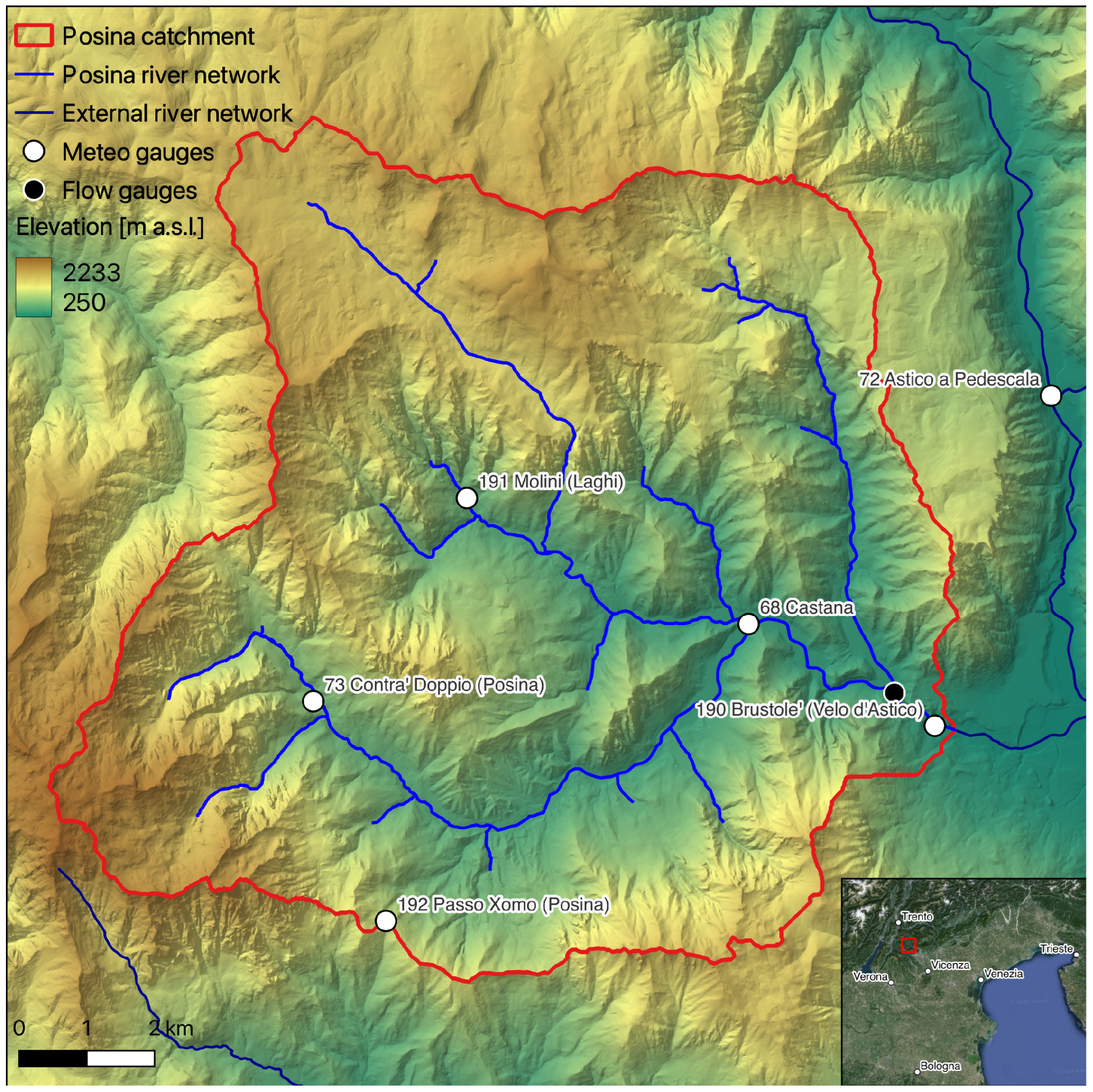
Figure 1. The Posina river network and its catchment.
Water 17 02341 g001
Figure 2. (a) October–November 2010 flood event. (b) October–November 2018 flood event.
Water 17 02341 g002
Figure 3. Long-term flow duration curve (FDC) based on historical data from January 2010 to July 2022.
Water 17 02341 g003
Figure 4. Rolling forecasting image depicts an example of the first four prediction instances of the rolling forecasting procedure that has been implemented. h refers to the previous hours of streamflow values used as input (cells with a red border), while m is the number of instances predicted at each inference (cells in dark and light blue). The green cells correspond to real measured values. The orange ones refer to predicted values used as input. The inference procedure moves as a sliding window. Therefore, at some point, the model will use only predicted values as input to compute the forecast for the next m values. The final forecast is obtained by combining the dark blue predicted values.
Water 17 02341 g004
Figure 5. LSTM model configuration. Yellow boxes show the input y ( t h ) streamflow values observed before the inference instance. X 1 and X k are the additional features used for the preceding h hours (streamflow, rainfall, and temperature) and the prediction of rainfall and temperature for the next m hours. y ^ reflects the streamflow values predicted in the subsequent m hours.
Water 17 02341 g005
Table 1. Models forecasting metrics performances on the testing set.
MetricARIMAXLSTMPhysically Based Hydrological Model
NSE [−]0.670.930.82
KGE [−]0.500.820.85
MAE [AVG m3/s]1.160.751.27
Disclaimer/Publisher’s Note: The statements, opinions and data contained in all publications are solely those of the individual author(s) and contributor(s) and not of MDPI and/or the editor(s). MDPI and/or the editor(s) disclaim responsibility for any injury to people or property resulting from any ideas, methods, instructions or products referred to in the content.