
An Approach to Improve Land–Water Salt Flux Modeling in the San Francisco Estuary


Abstract
1. Introduction
2. Background
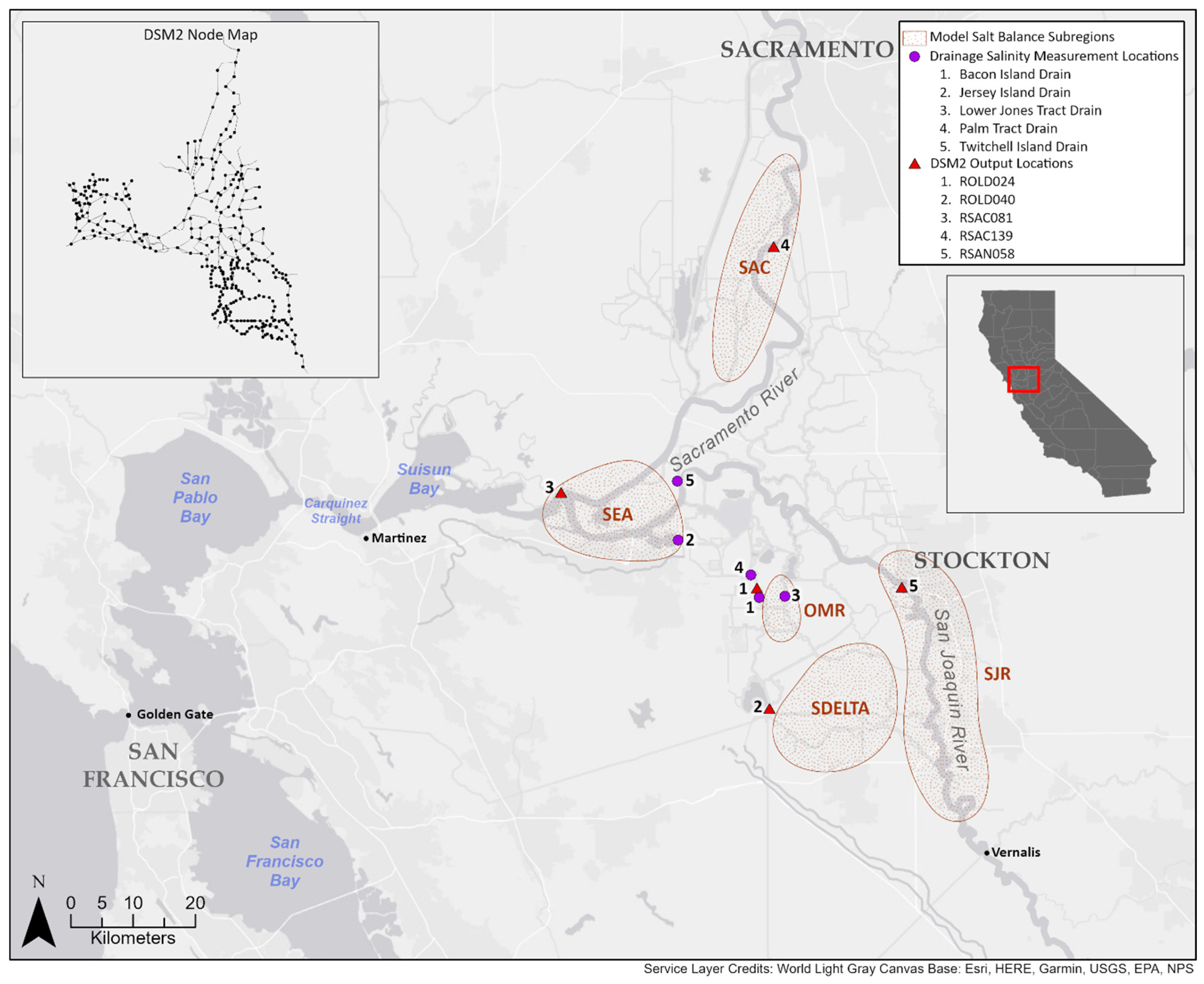
2.1. Study Area
2.2. DSM2 Model and Island Salt Flux Representation
3. Methods
3.1. Model Subregion Delineation
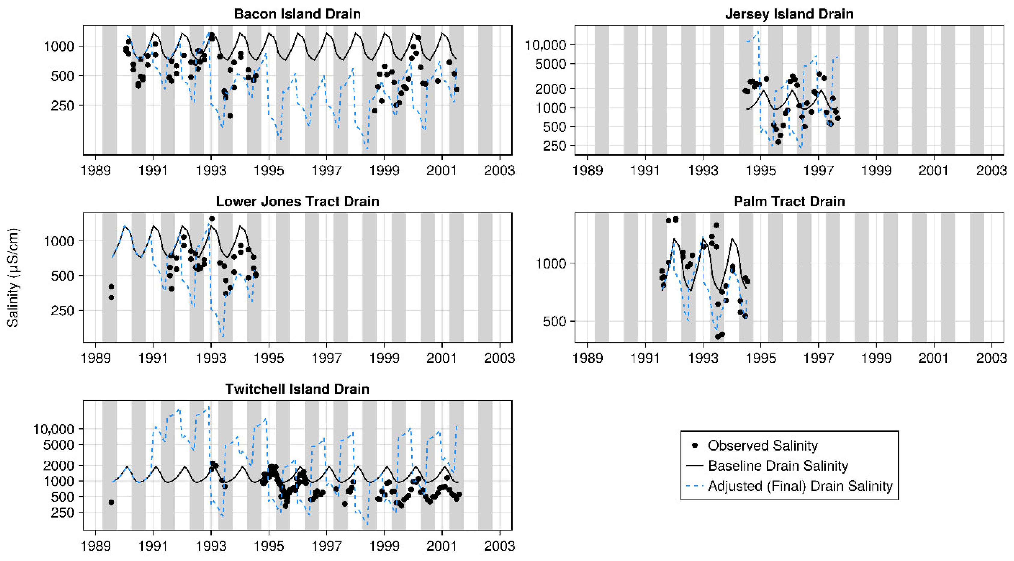
3.2. Observed Drainage Salinity Data
3.3. Modeling Approach
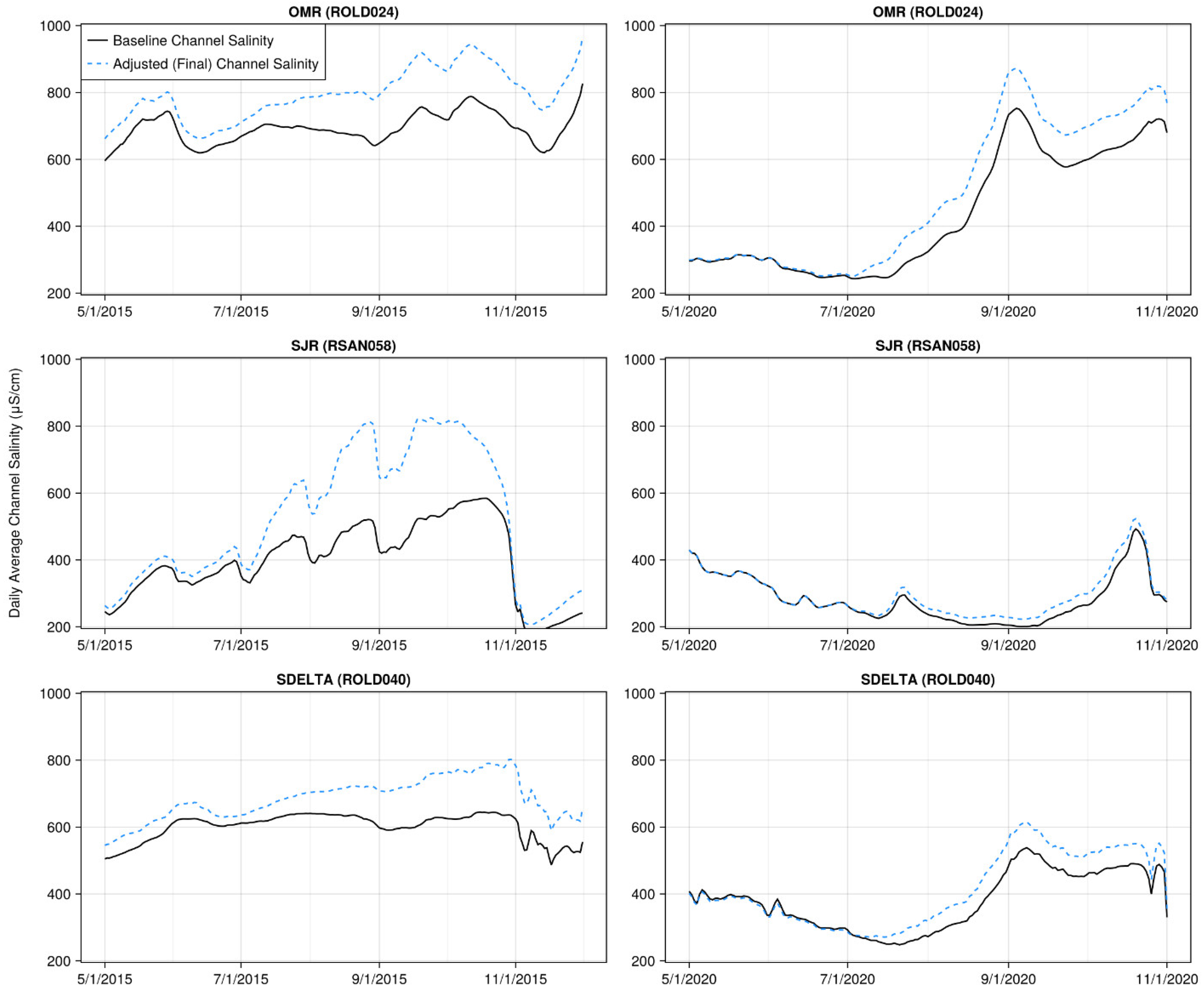
4. Results
5. Discussion
Author Contributions
Funding
Data Availability Statement
Conflicts of Interest
References
- California Department of Water Resources (CDWR). DSM2: Delta Simulation Model II. 2021. Available online: https://water.ca.gov/Library/Modeling-and-Analysis/Bay-Delta-Region-models-and-tools/Delta-Simulation-Model-II (accessed on 20 June 2023).
- Martyr-Koller, R.C.; Kernkamp, H.W.J.; Van Dam, A.; van der Wegen, M.; Lucas, L.V.; Knowles, N.; Jaffe, B.; Fregoso, T.A. Application of an unstructured 3D finite volume numerical model to flows and salinity dynamics in the San Francisco Bay-Delta. Estuar. Coast. Shelf Sci. 2017, 192, 86–107. [Google Scholar] [CrossRef]
- MacWilliams, M.L.; Bever, A.J.; Gross, E.S.; Ketefian, G.S.; Kimmerer, W.J. Three-dimensional modeling of hydrodynamics and salinity in the San Francisco estuary: An evaluation of model accuracy, X2, and the low–salinity zone. San Fr. Estuary Watershed Sci. 2015, 13. [Google Scholar] [CrossRef]
- Ateljevich, E.; Nam, K.; Zhang, Y.J.; Wang, R.; Shu, Q. Bay-delta SELFE calibration overview. In 35th Annual Progress Report to the State Water Resources Control Board, Methodology for Flow and Salinity Estimates in the Sacramento-San Joaquin Delta and Suisun Marsh; CDWR: Sacramento, CA, USA, 2014. [Google Scholar]
- California Water and Environmental Modeling Forum (CWEMF). RMA2–Model Inventory. Prepared for the Delta Stewardship Council. 2018. Available online: https://cwemfwiki.atlassian.net/wiki/spaces/MI/pages/147062807/RMA2 (accessed on 1 April 2025).
- CDWR. Quantity and Quality of Waters Applied to and Drained from the Delta Lowlands, Investigations of the Sacramento-San Joaquin Delta, Report No. 4; CDWR: Sacramento, CA, USA, 1956. [Google Scholar]
- Roy, S.; Hutton, P.; Heidel, K.; Grieb, T.; Tasdighi, A. Integrated Modeling in the Delta: Status, Challenges and a View to the Future, prepared for the Delta Stewardship Council; Delta Stewardship Council: Sacramento, CA, USA, 2020. [Google Scholar]
- Moyle, P.B.; Lund, J.R.; Bennett, W.A.; Fleenor, W.E. Habitat variability and complexity in the upper San Francisco Estuary. San Fr. Estuary Watershed Sci. 2010, 8. [Google Scholar] [CrossRef]
- Cloern, J.E.; Jassby, A.D. Drivers of change in estuarine-coastal ecosystems: Discoveries from four decades of study in San Francisco Bay. Rev. Geophys. 2012, 50. [Google Scholar] [CrossRef]
- Lund, J.; Hanak, E.; Fleenor, W.; Bennett, W.; Howitt, R. Comparing Futures for the Sacramento, San Joaquin Delta; University of California Press: Oakland, CA, USA, 2010; Volume 3. [Google Scholar]
- Deverel, S.J.; Leighton, D.A. Historic, recent, and future subsidence, Sacramento-San Joaquin Delta, California, USA. San Fr. Estuary Watershed Sci. 2010, 8. [Google Scholar] [CrossRef]
- Ariyama, J.; Boisrame, G.F.S.; Brand, M.R. Water Budgets for the Delta Watershed: Putting Together the Many Disparate Pieces. San Fr. Estuary Watershed Sci. 2019, 17. [Google Scholar] [CrossRef]
- Hutton, P.H.; Rath, J.S.; Ateljevich, E.S.; Roy, S.B. Apparent Seasonal Bias in Delta Outflow Estimates as Revealed in the Historical Salinity Record of the San Francisco Estuary: Implications for Delta Net Channel Depletion Estimates. San Fr. Estuary Watershed Sci. J. 2021, 19. [Google Scholar] [CrossRef]
- Amy, G.L.; Thompson, J.M.; Tan, L.; Davis, M.K.; Krasner, S.W. Evaluation of THM Precursor Contributions from Agricultural Drains. J. Am. Water Work. Assoc. 1990, 82, 57–64. [Google Scholar] [CrossRef]
- Hutton, P.H.; Chung, F.I. Simulating THM Formation Potential in Sacramento Delta, Part I., Journal Water Resources Planning and Management. Am. Soc. Civ. Eng. 1992, 118, 530–542. [Google Scholar]
- Hutton, P.H.; Roy, S.B.; Krasner, S.W.; Palencia, L. The Municipal Water Quality Investigations Program: A Retrospective Overview of the Program’s First Three Decades. Water 2022, 14, 3426. [Google Scholar] [CrossRef]
- CDWR. DCD: Delta Channel Depletion. 2018. Available online: https://water.ca.gov/Library/Modeling-and-Analysis/Bay-Delta-Region-models-and-tools/DCD (accessed on 20 June 2023).
- Jung, M. Revision of Representative Delta Island Return Flow Quality for DSM2 and DICU Model Runs, Consultant’s Report Prepared for CDWR’s MWQI Program; Marvin Jung & Associates, Inc.: Sacramento, CA, USA, 2000. [Google Scholar]
- Hutton, P.H.; Sinha, A.; Roy, S.B.; Denton, R.A. A Simplified Approach for Estimating Ionic Concentrations from Specific Conductance Data in the San Francisco Estuary. San Fr. Estuary Watershed Sci. J. 2023, 21. [Google Scholar] [CrossRef]
- Hem, J.D. Study and Interpretation of the Chemical Characteristics of Natural Water, USGS Water Supply Paper 2254, Third Edition. 1985. Available online: https://pubs.usgs.gov/wsp/wsp2254/pdf/wsp2254a.pdf (accessed on 1 April 2025).
- Denton, R.A. Delta Salinity Constituent Analysis, Report Prepared for the State Water Project Contractors Authority, February. 2015. Available online: https://rtdf.info/ (accessed on 10 June 2023).
- Andrews, S.; Gross, E.; Hutton, P.H. Modeling Salt Intrusion in the San Francisco Estuary Prior to Anthropogenic Influence. Cont. Shelf Res. 2017, 146, 58–81. [Google Scholar] [CrossRef]
- Hutton, P.H.; Rath, J.; Chen, L.; Ungs, M.L.; Roy, S.B. Nine Decades of Salinity Observations in the San Francisco Bay and Delta: Modeling and Trend Evaluation. J. Water Resour. Plan. Manag. 2015. [Google Scholar] [CrossRef]
- Hutton, P.H.; Roy, S.B. Characterizing Early 20th Century Delta Outflow and Salinity Intrusion in the San Francisco Estuary. San Fr. Estuary Watershed Sci. J. 2019, 17. [Google Scholar]


| Model Subregion | Acronym | General Description |
|---|---|---|
| Freshwater Boundary | SAC | main stem of the Sacramento River upstream of the confluence with the San Joaquin River |
| Seaward Boundary | SEA | confluence of the Sacramento and San Joaquin Rivers |
| Old-Middle River Export Corridor | OMR | a region uniquely influenced by hydrodynamic patterns driven by State Water Project and Central Valley Project diversions from the Delta |
| San Joaquin River Corridor | SJR | main stem of the San Joaquin River downstream of Vernalis |
| South Delta | SDELTA | a region uniquely influenced by salt loads that enter the Delta at Vernalis, the placement of seasonal in-channel rock barriers, and local sources of salinity (including agricultural drainage and groundwater) |
| Location | Dates | # Data Points |
|---|---|---|
| Twitchell Island Drain | 19 July 1989–6 August 2001 | 127 |
| Jersey Island Drain | 20 June 1994–2 September 1997 | 34 |
| Palm Tract Drain | 31 July 1991–18 July 1994 | 32 |
| Bacon Island Drain | 23 January 1990–3 July 2001 | 78 |
| Lower Jones Tract Drain | 19 July 1989–19 July 1994 | 36 |
| Step | Step Title | Step Description |
|---|---|---|
| 1 | Run hydrodynamic model | Run DSM2 HYDRO module |
| 2 | Run salinity transport model | Run DSM2 QUAL module |
| 3 | Compute subregional salt mass fluxes | For each node in a given subregion, add up the inflowing and outflowing salt masses |
| 4 | Convert EC to mg/L | Based on broad natural water characteristics reported in [20] and local conditions reported in [21] assume 1 μS/cm = 0.6 mg/L |
| 5 | Convert to tons of salt mass | 1 ac × ft of water with 1 mg/L salinity = 0.000815808 t |
| 6 | Compute mass balance deficit | Over 6-month time windows, compute the difference between inflows and outflow salt masses |
| 7 | Adjust deficit by heuristic factors | Multiply a subregion-specific heuristic factor (SAC = 1.3, SEA = 0.95, OMR = 1.1, SJR = 1.0, SDELTA = 1.0) to each salt balance deficit |
| 8 | Update boundary conditions | Distributed the adjusted mass deficit offset uniformly over the 6-month time window |
| 9 | Iterate until approximate convergence | Return to step 2, repeat as necessary until estimates no longer substantially change (4 repetitions were necessary in this case) |
Disclaimer/Publisher’s Note: The statements, opinions and data contained in all publications are solely those of the individual author(s) and contributor(s) and not of MDPI and/or the editor(s). MDPI and/or the editor(s) disclaim responsibility for any injury to people or property resulting from any ideas, methods, instructions or products referred to in the content. |
© 2025 by the authors. Licensee MDPI, Basel, Switzerland. This article is an open access article distributed under the terms and conditions of the Creative Commons Attribution (CC BY) license (https://creativecommons.org/licenses/by/4.0/).
Share and Cite
Rath, J.S.; Hutton, P.H.; Roy, S.B. An Approach to Improve Land–Water Salt Flux Modeling in the San Francisco Estuary. Water 2025, 17, 2278. https://doi.org/10.3390/w17152278
Rath JS, Hutton PH, Roy SB. An Approach to Improve Land–Water Salt Flux Modeling in the San Francisco Estuary. Water. 2025; 17(15):2278. https://doi.org/10.3390/w17152278
Chicago/Turabian StyleRath, John S., Paul H. Hutton, and Sujoy B. Roy. 2025. "An Approach to Improve Land–Water Salt Flux Modeling in the San Francisco Estuary" Water 17, no. 15: 2278. https://doi.org/10.3390/w17152278
APA StyleRath, J. S., Hutton, P. H., & Roy, S. B. (2025). An Approach to Improve Land–Water Salt Flux Modeling in the San Francisco Estuary. Water, 17(15), 2278. https://doi.org/10.3390/w17152278