Figure 1.
Salento peninsula main geology, location of the sampling wells, rain gauges, and stratigraphic.
Figure 1.
Salento peninsula main geology, location of the sampling wells, rain gauges, and stratigraphic.
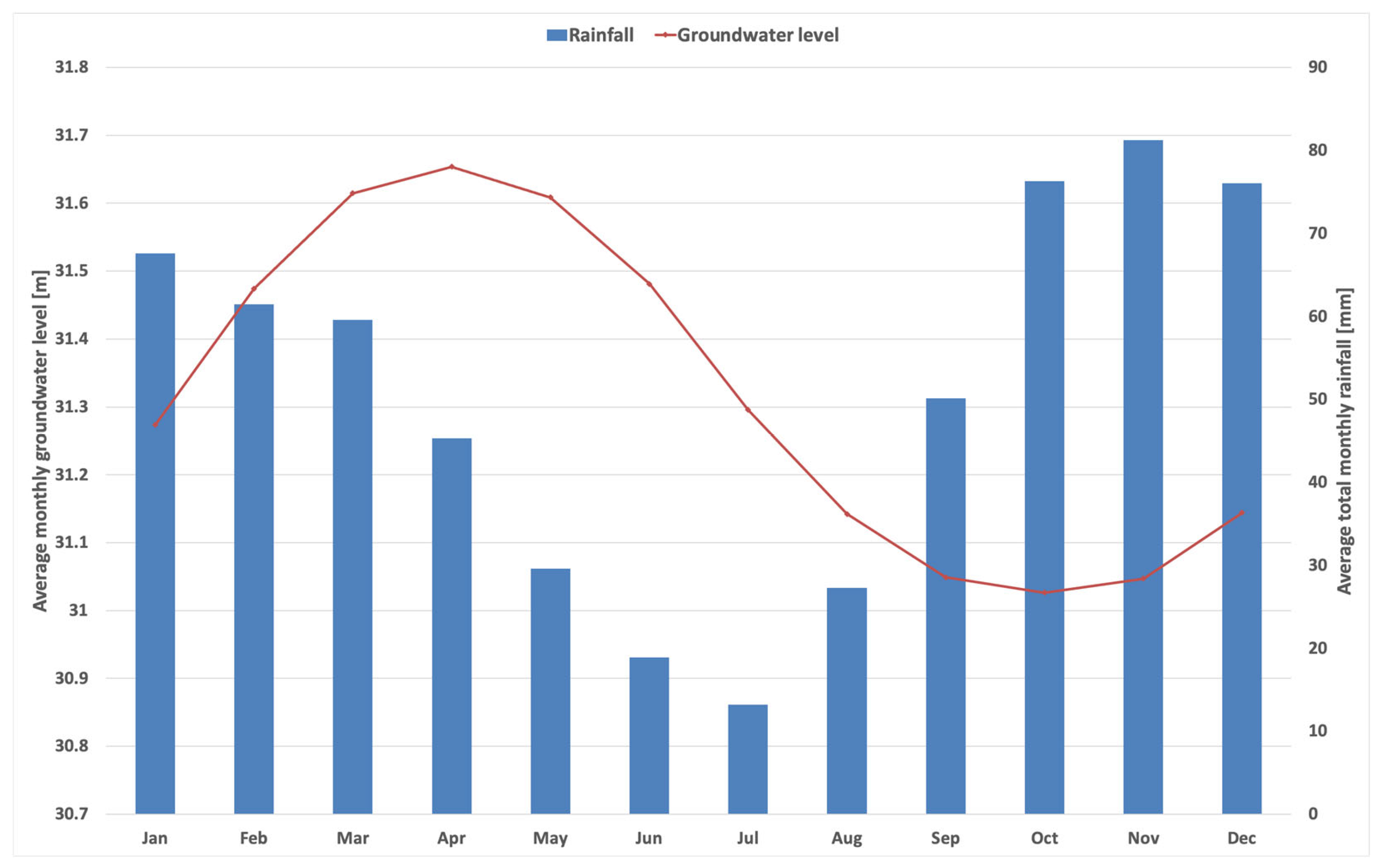
Figure 2.
Average monthly water table levels of Brindisi shallow aquifer and average precipitation of Brindisi rain-gauge station, estimate for the time.
Figure 2.
Average monthly water table levels of Brindisi shallow aquifer and average precipitation of Brindisi rain-gauge station, estimate for the time.
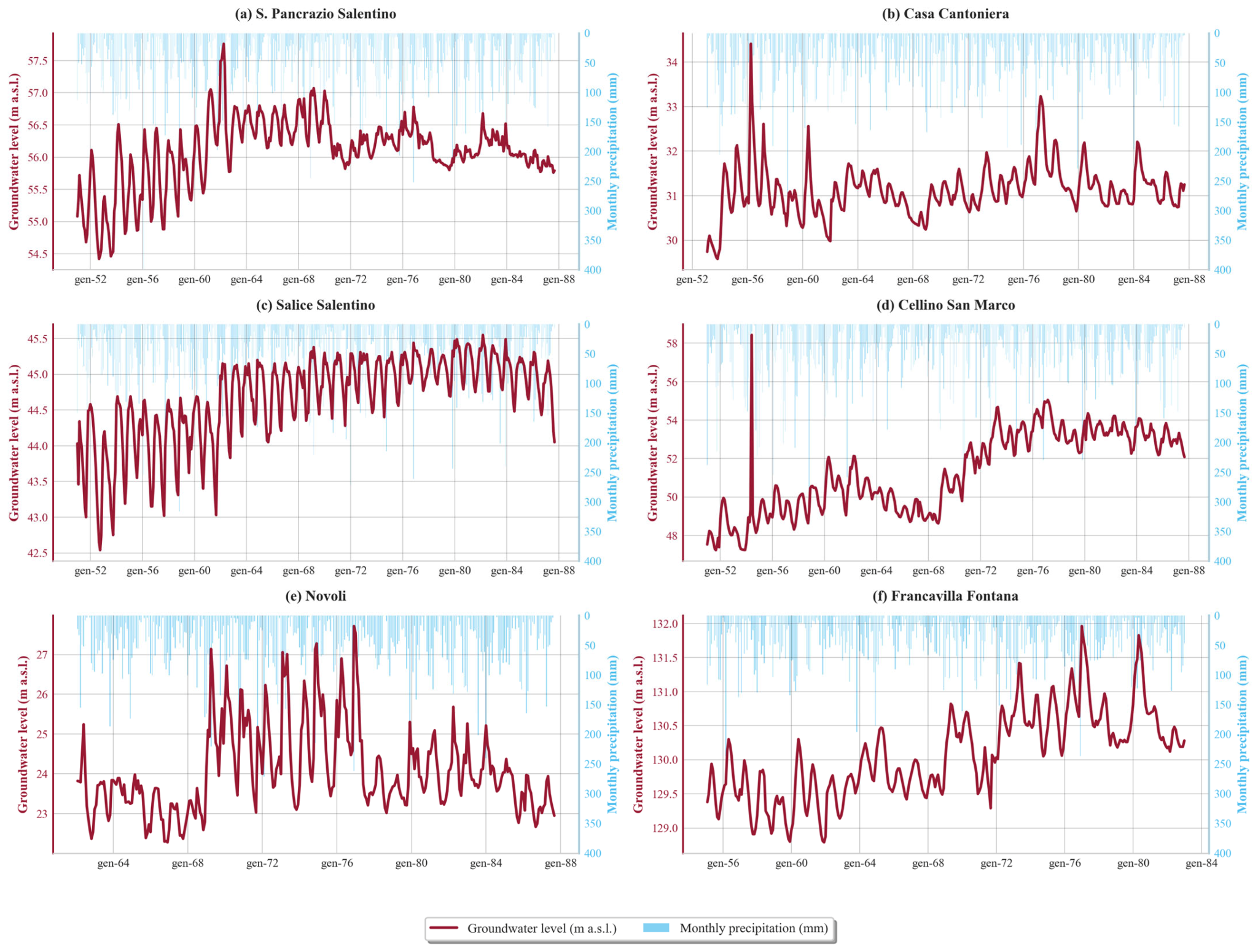
Figure 3.
Historical Groundwater Level and Monthly Precipitation Time Series for the Six Study Wells. Each panel (a–f) shows the long-term variations in groundwater level (red line, left y-axis, measured in meters above sea level (m a.s.l.)) and corresponding monthly precipitation (light blue bars, right y-axis, measured in millimeters [mm]). The toponyms of wells are the following: (a) S. Pancrazio Salentino, (b) Casa Cantoniera, (c) Salice Salentino, (d) Cellino San Marco, (e) Novoli, and (f) Francavilla Fontana.
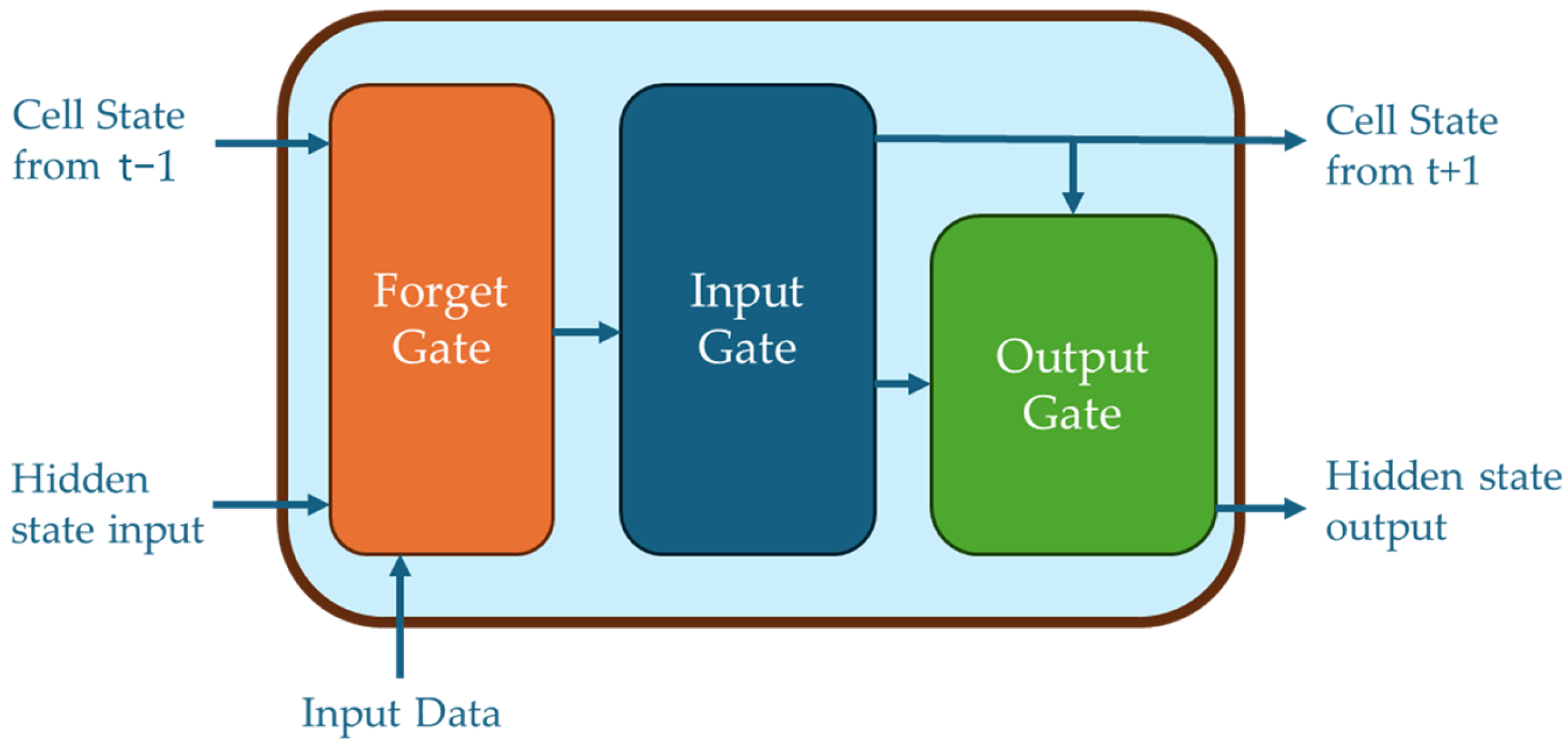
Figure 4.
Schematic representation of an LSTM cell.
Figure 4.
Schematic representation of an LSTM cell.
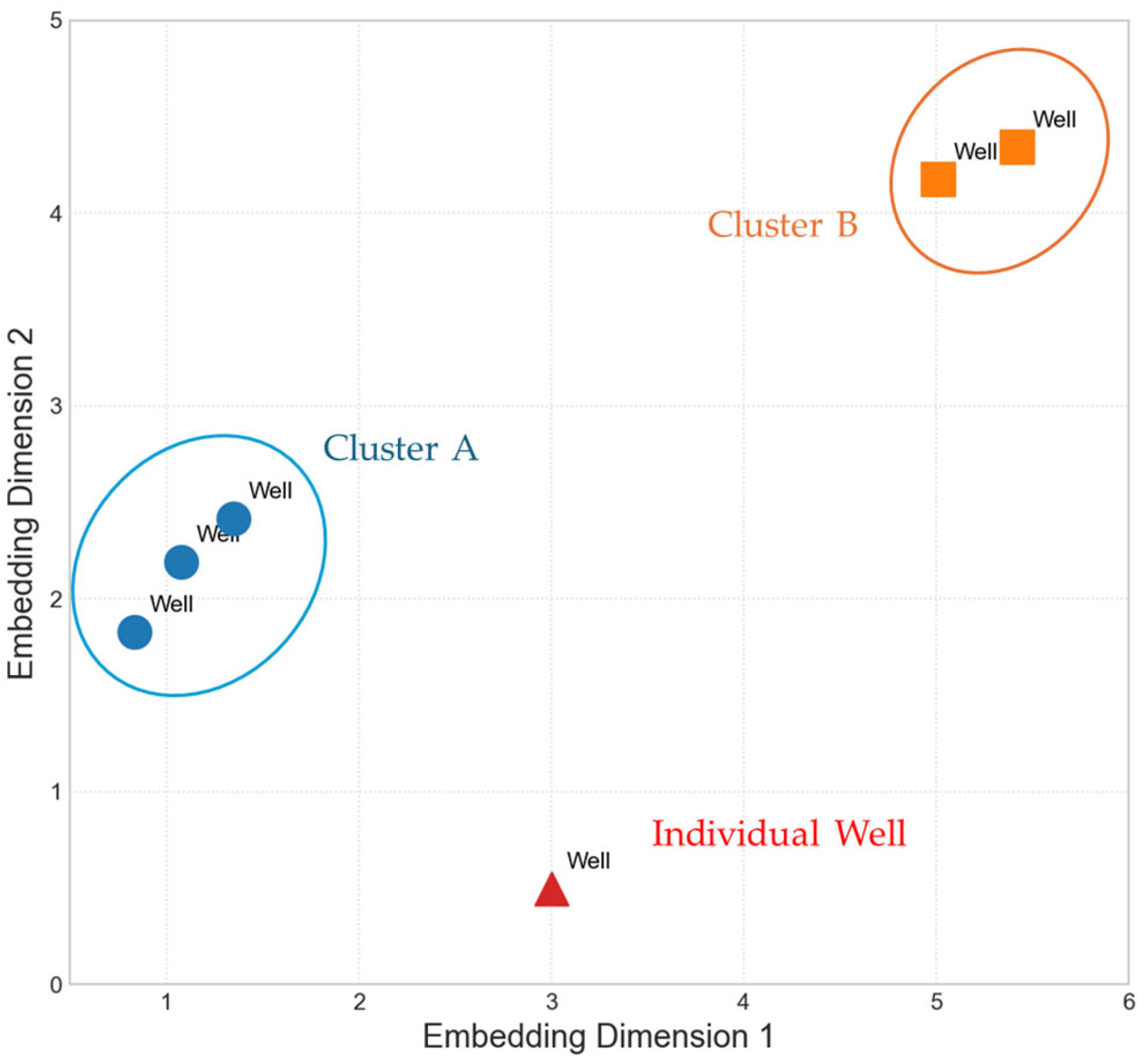
Figure 5.
Example of scatter plot representation of well identifiers in a 2D embedding space. Cluster A (orange circle) wells are grouped due to their learned similarities, while Cluster B wells form another distinct similar group but are distant from Cluster A (blue circle). An Individual Well (red triangle).
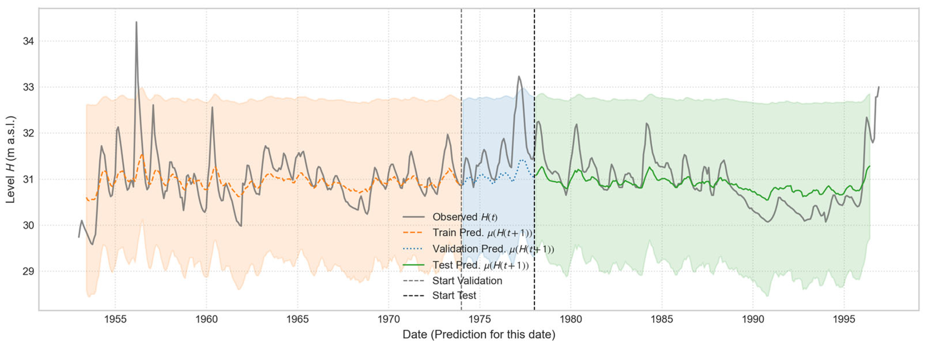
Figure 6.
One month ahead Open-Loop prediction for “Casa Cantoniera” well, generated by the individually trained model.
Figure 6.
One month ahead Open-Loop prediction for “Casa Cantoniera” well, generated by the individually trained model.
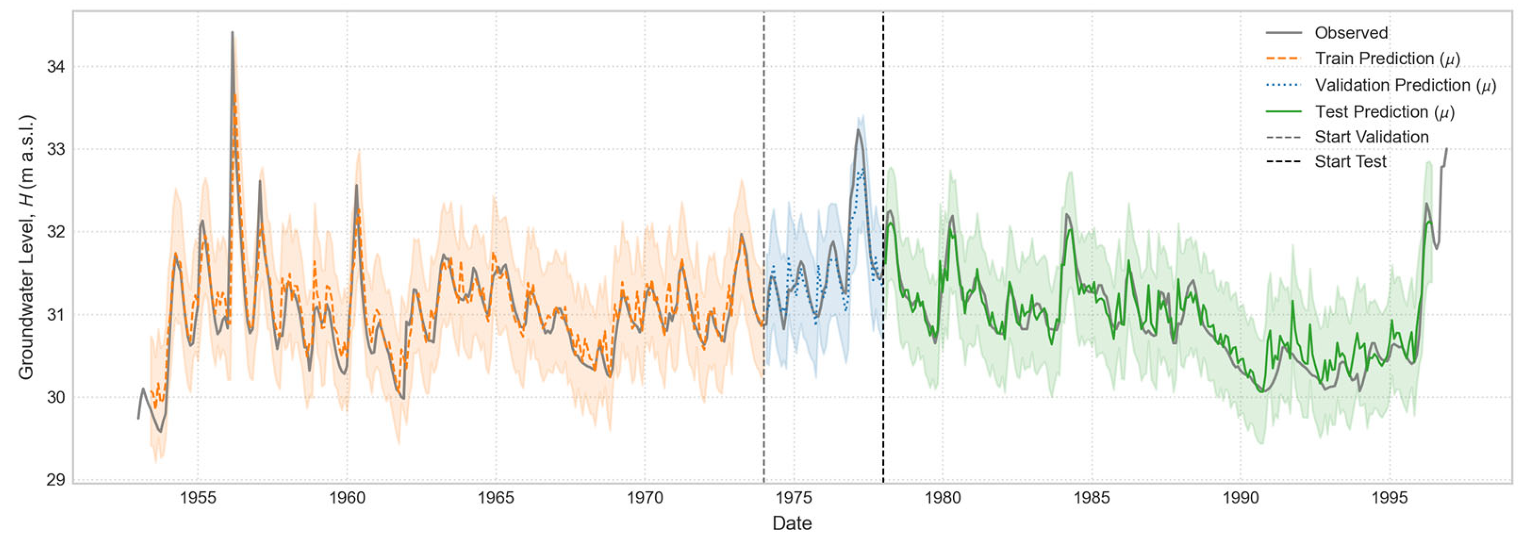
Figure 7.
One month ahead Open-Loop prediction for “Casa Cantoniera” well, generated by the globally trained model.
Figure 7.
One month ahead Open-Loop prediction for “Casa Cantoniera” well, generated by the globally trained model.
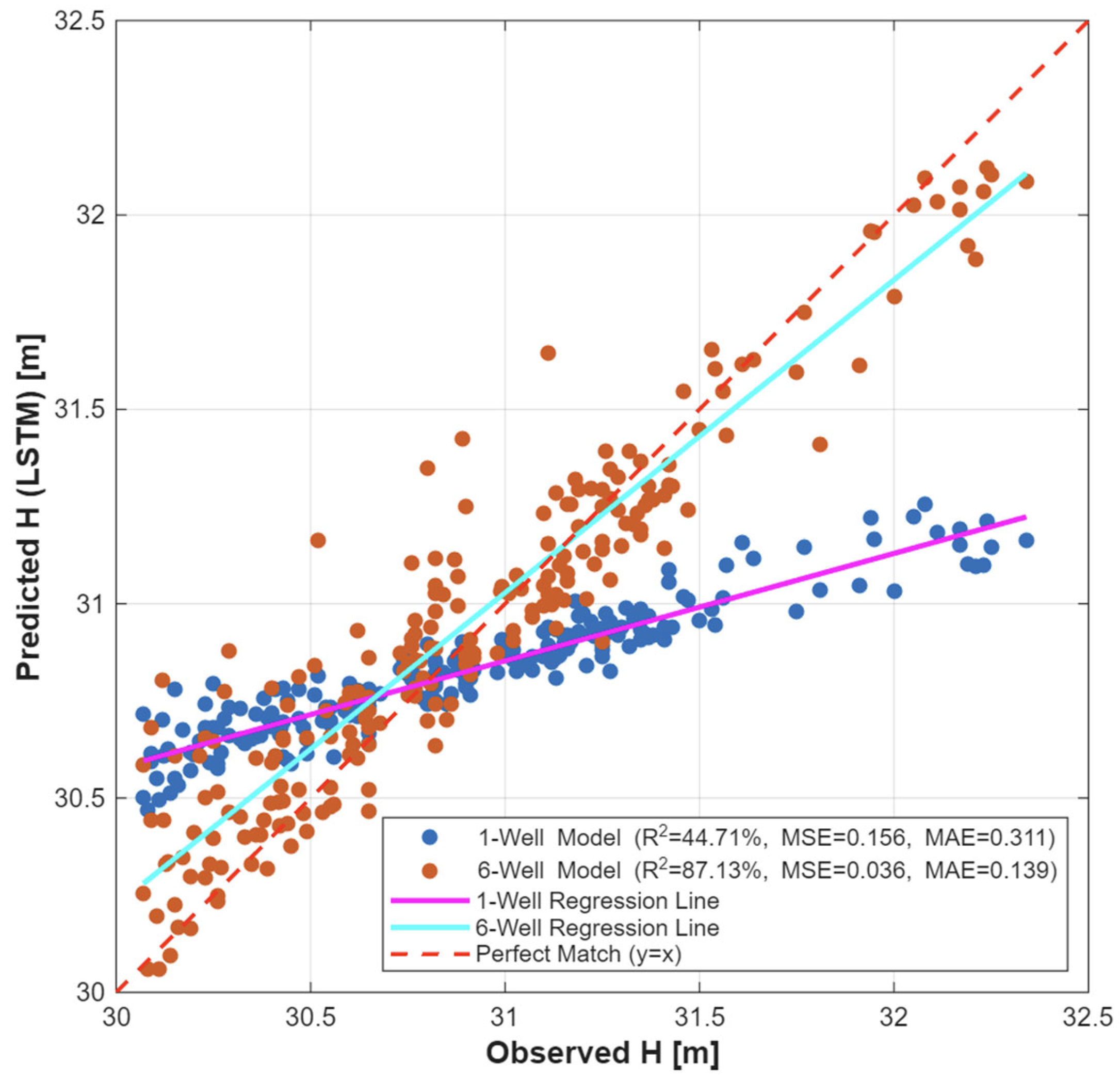
Figure 8.
Scatter plot: In blue, the one month ahead Open-Loop prediction for “Casa Cantoniera” well, generated by the individually trained model; in red, one month ahead Open-Loop prediction for “Casa Cantoniera” well, generated by the globally trained model.
Figure 8.
Scatter plot: In blue, the one month ahead Open-Loop prediction for “Casa Cantoniera” well, generated by the individually trained model; in red, one month ahead Open-Loop prediction for “Casa Cantoniera” well, generated by the globally trained model.
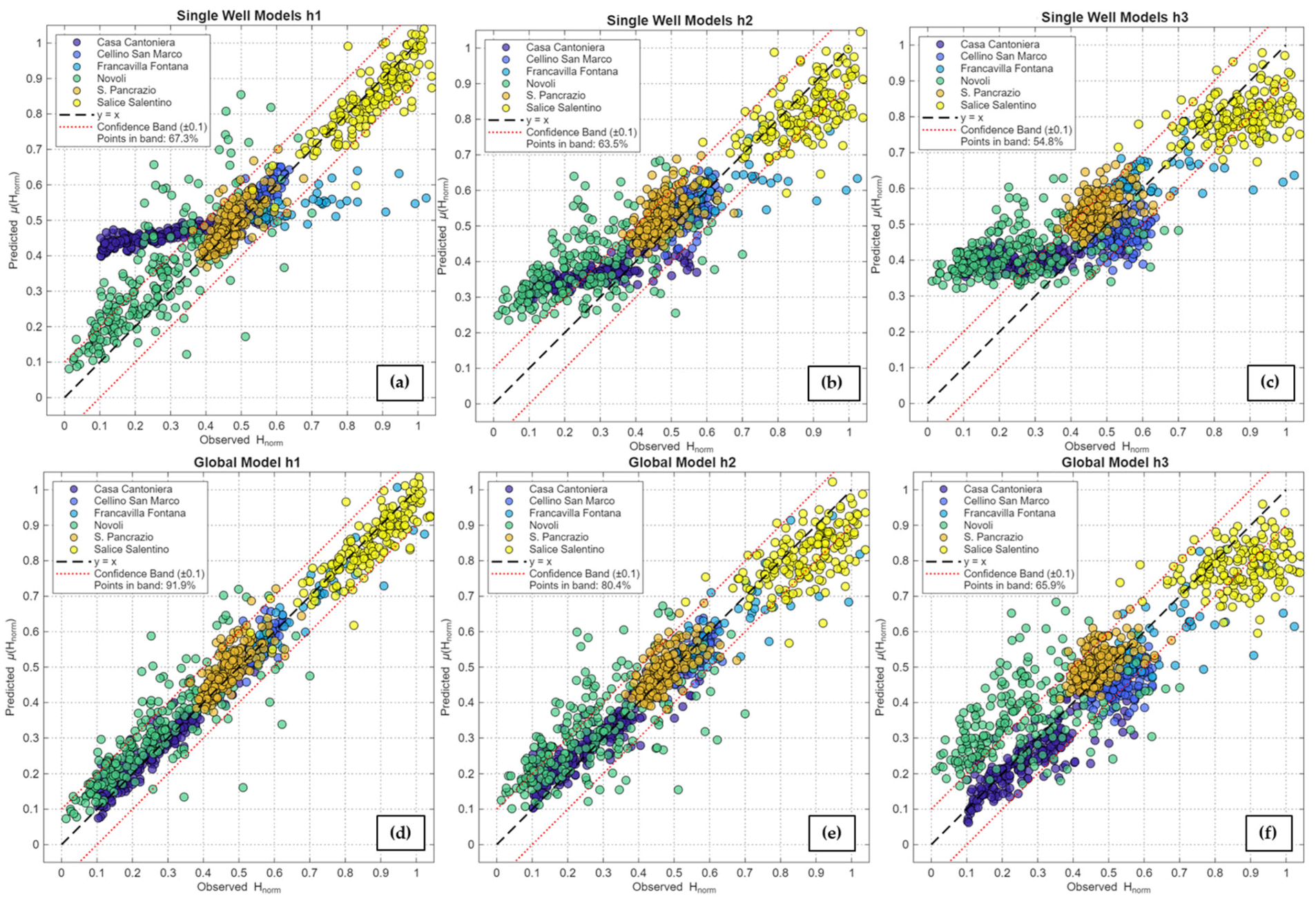
Figure 9.
Scatter plots of the Open-Loop predictions at different forecast horizons (h1, h2, h3). The plots compare the observed normalized groundwater level values (x-axis) with the predicted values (y-axis). The top row (a–c) illustrates the performance of the models trained individually on each well (‘Single Well Models’), while the bottom row (d–f) refers to the global model (‘Global Model’) trained on all wells simultaneously. The columns represent forecast horizons of one (h1), two (h2), and three (h3) months. The black dashed line indicates perfect agreement (y = x), and the red lines define a confidence band of ±0.1.
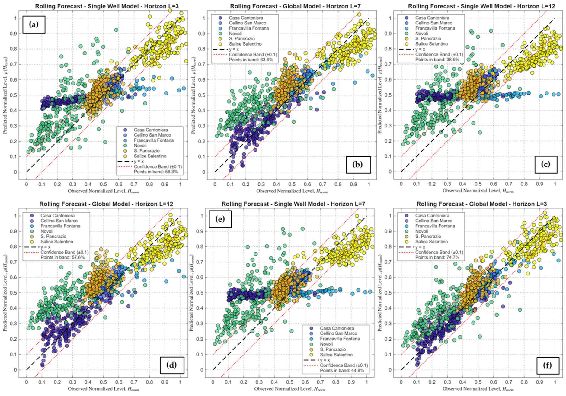
Figure 10.
Scatter plots of the Rolling Forecast predictions at different forecast horizons. Plots (a–c) illustrate the performance of the models trained individually on each well (‘Single Well Model’) for forecast horizons of L = 3, L = 7, and L = 12. Plots (d–f) refer to the global model (‘Global Model’), trained on all wells simultaneously, for the same forecast horizons. The black dashed line indicates perfect agreement (y = x), while the red lines define a confidence band of ±0.1.
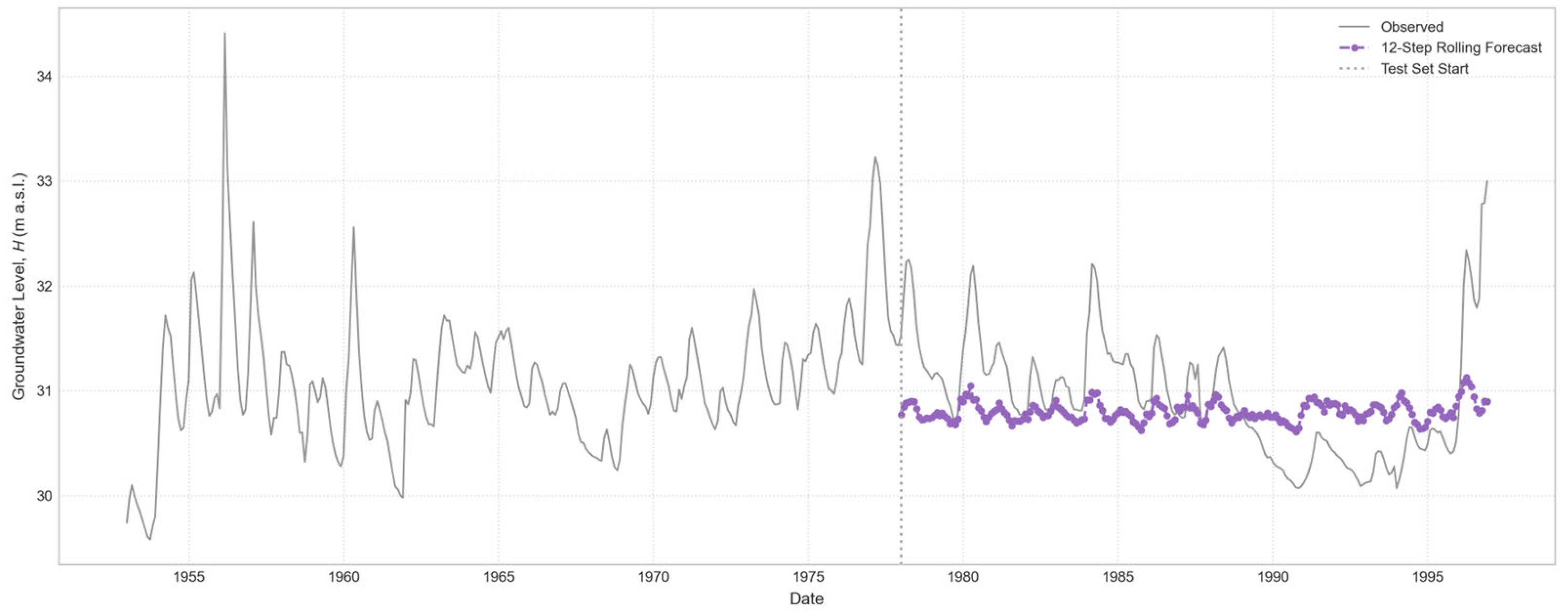
Figure 11.
12-step horizon rolling multi-step forecast for “Casa Cantoniera” well, generated by the individually trained model.
Figure 11.
12-step horizon rolling multi-step forecast for “Casa Cantoniera” well, generated by the individually trained model.
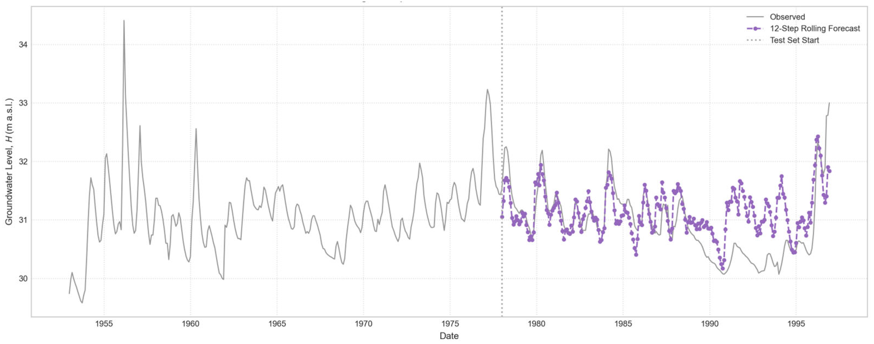
Figure 12.
12-step horizon rolling multi-step forecast for “Casa Cantoniera” well, generated by the globally trained model.
Figure 12.
12-step horizon rolling multi-step forecast for “Casa Cantoniera” well, generated by the globally trained model.
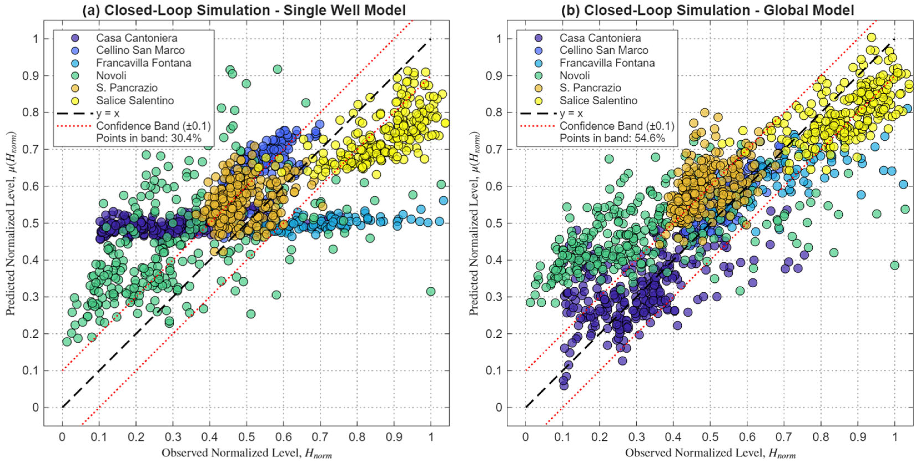
Figure 13.
Scatter plots comparing the performance of the models in Closed-Loop Simulation. The plots show the observed normalized values (Hnorm) on the x-axis versus the predicted values on the y-axis. (a) illustrates the results for the Single Well Model (trained on each well individually), while (b) shows the results for the Global Model (trained on all wells simultaneously). The black dashed line indicates perfect agreement (y = x), and the red lines define a confidence band of ±0.1.
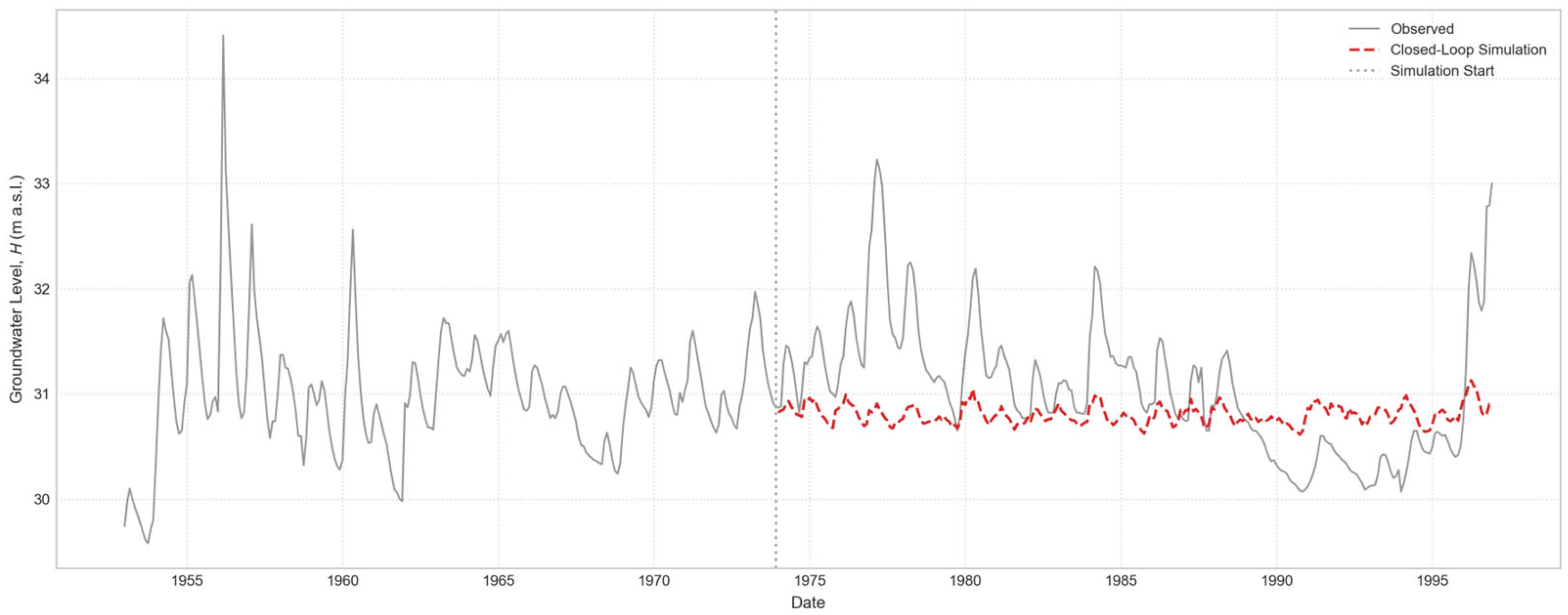
Figure 14.
Closed-Loop simulation forecast for “Casa Cantoniera” well, generated by the individually trained model.
Figure 14.
Closed-Loop simulation forecast for “Casa Cantoniera” well, generated by the individually trained model.
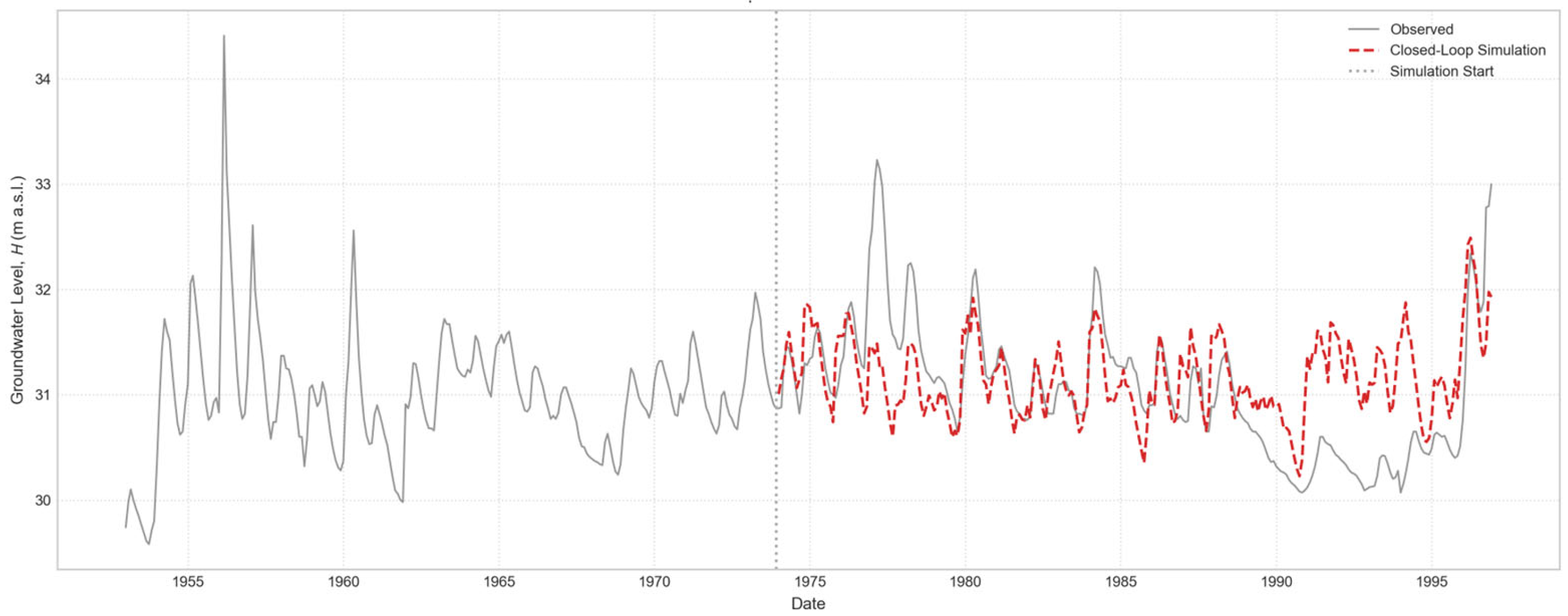
Figure 15.
Closed-Loop simulation forecast for “Casa Cantoniera” well, generated by the globally trained model.
Figure 15.
Closed-Loop simulation forecast for “Casa Cantoniera” well, generated by the globally trained model.
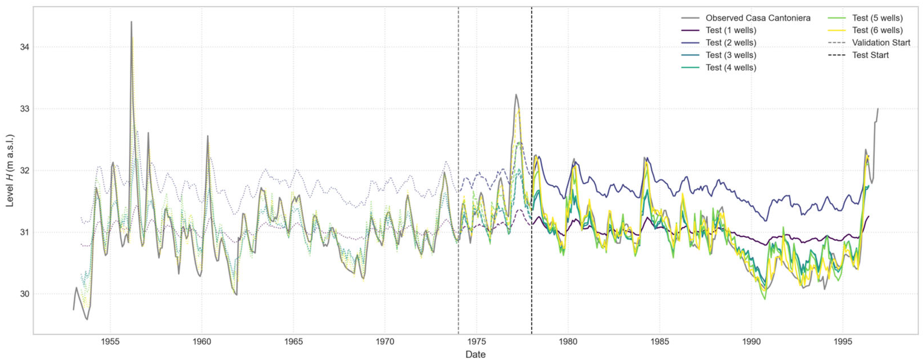
Figure 16.
Comparison of Open-Loop predictions for the “Casa Cantoniera” well, with a 1-month forecast horizon. The plot illustrates the performance of a series of models, each trained using an increasing number of input wells, from one to six.
Figure 16.
Comparison of Open-Loop predictions for the “Casa Cantoniera” well, with a 1-month forecast horizon. The plot illustrates the performance of a series of models, each trained using an increasing number of input wells, from one to six.
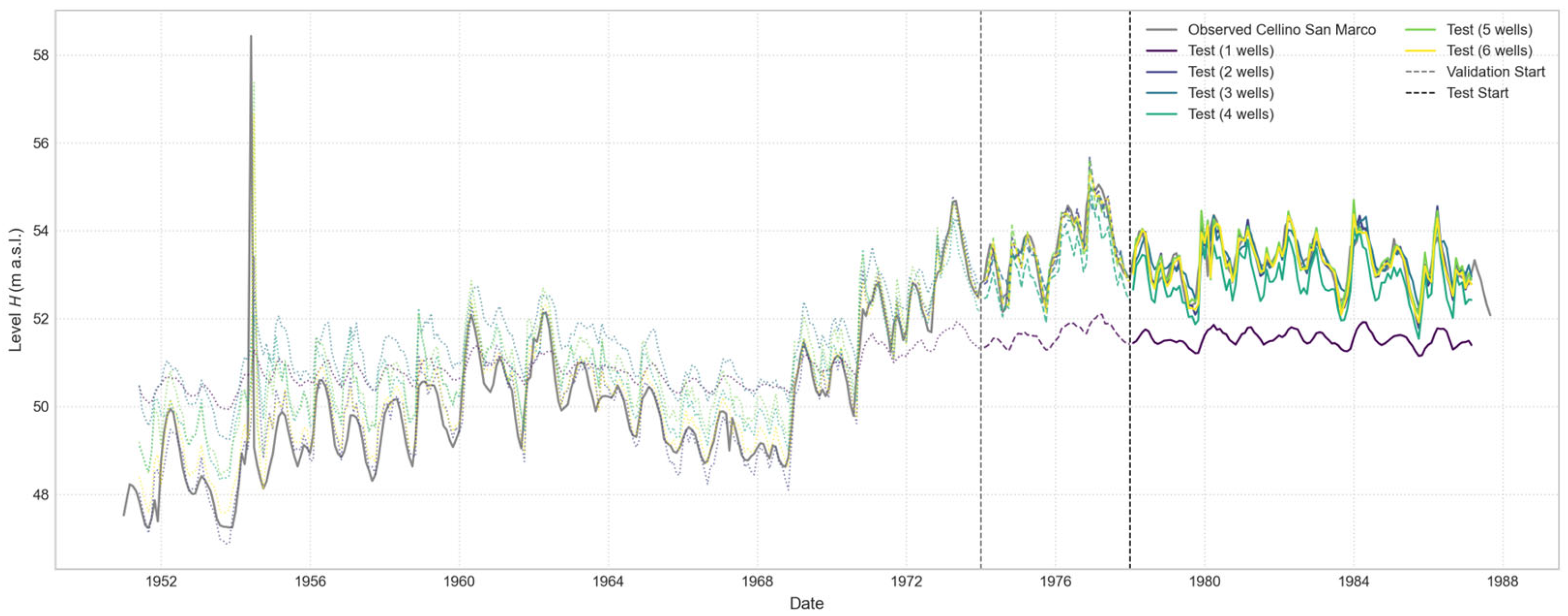
Figure 17.
Comparison of Open-Loop predictions for the “Cellino San Marco” well, with a 1-month forecast horizon. The plot illustrates the performance of a series of models, each trained using an increasing number of input wells, from one to six.
Figure 17.
Comparison of Open-Loop predictions for the “Cellino San Marco” well, with a 1-month forecast horizon. The plot illustrates the performance of a series of models, each trained using an increasing number of input wells, from one to six.
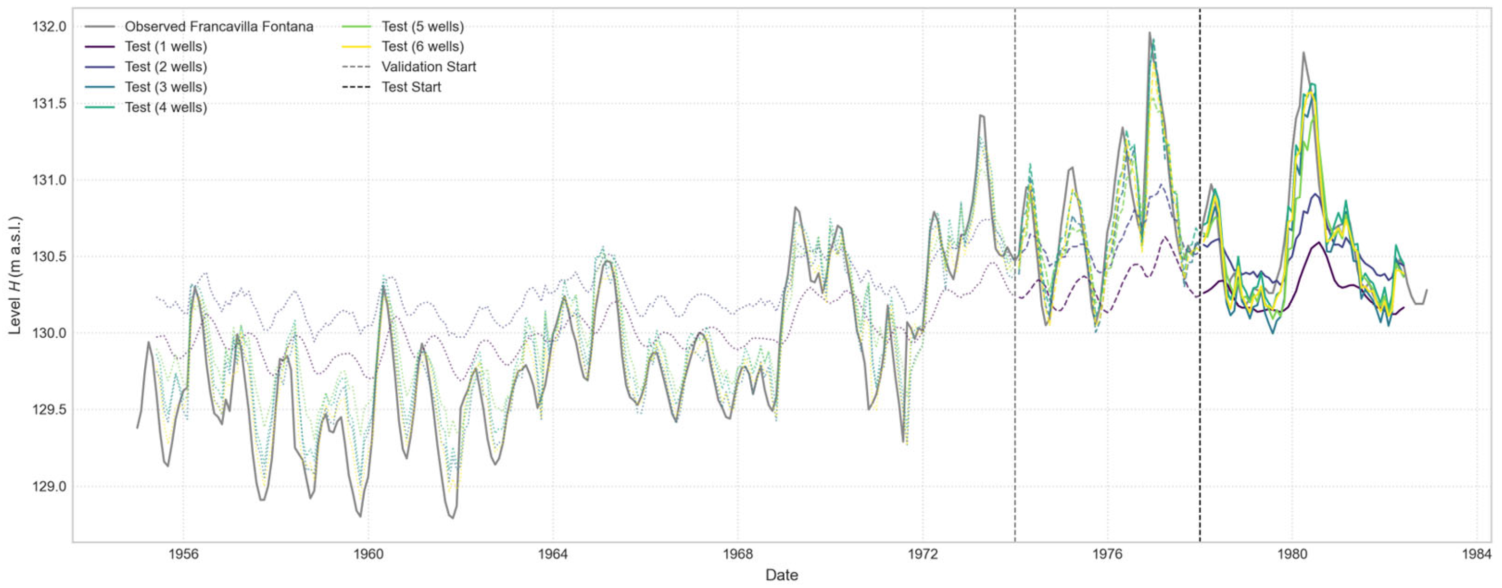
Figure 18.
Comparison of Open-Loop predictions for the “Francavilla Fontana” well, with a 1-month forecast horizon. The plot illustrates the performance of a series of models, each trained using an increasing number of input wells, from one to six.
Figure 18.
Comparison of Open-Loop predictions for the “Francavilla Fontana” well, with a 1-month forecast horizon. The plot illustrates the performance of a series of models, each trained using an increasing number of input wells, from one to six.
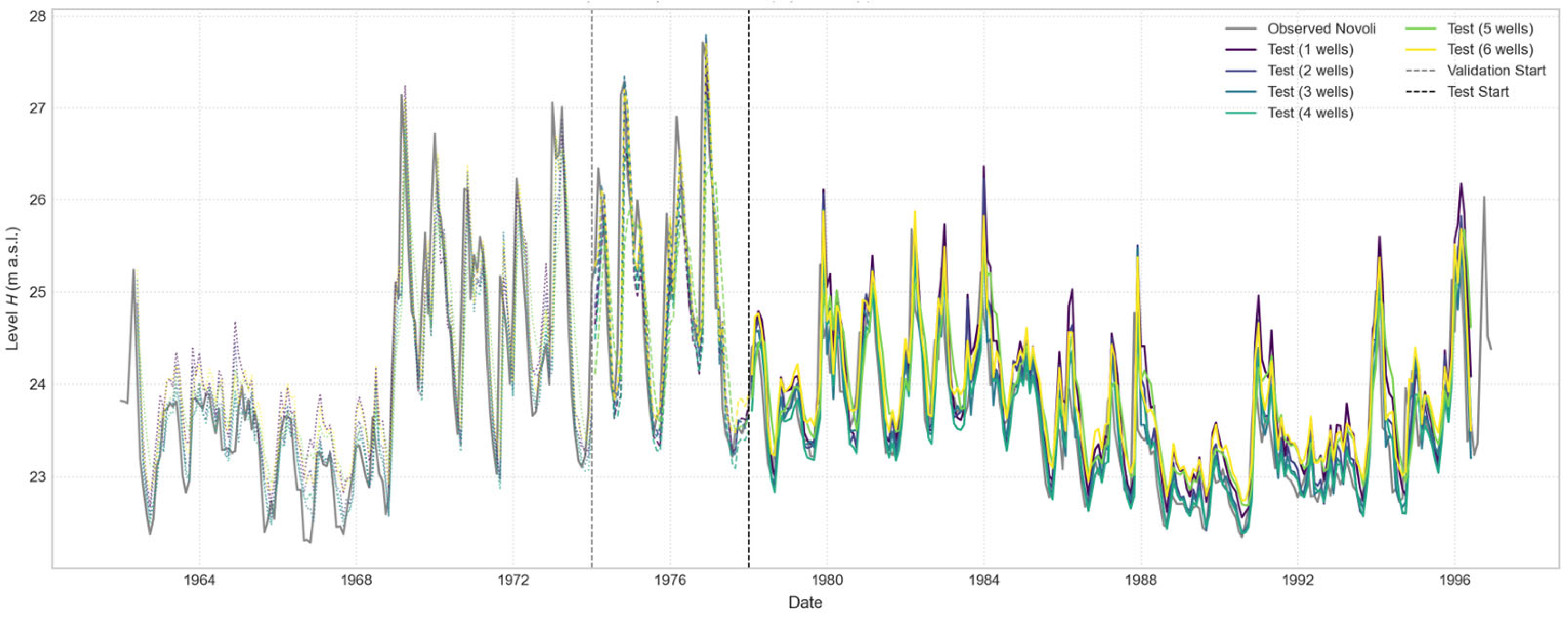
Figure 19.
Comparison of Open-Loop predictions for the “Novoli” well, with a 1-month forecast horizon. The plot illustrates the performance of a series of models, each trained using an increasing number of input wells, from one to six.
Figure 19.
Comparison of Open-Loop predictions for the “Novoli” well, with a 1-month forecast horizon. The plot illustrates the performance of a series of models, each trained using an increasing number of input wells, from one to six.
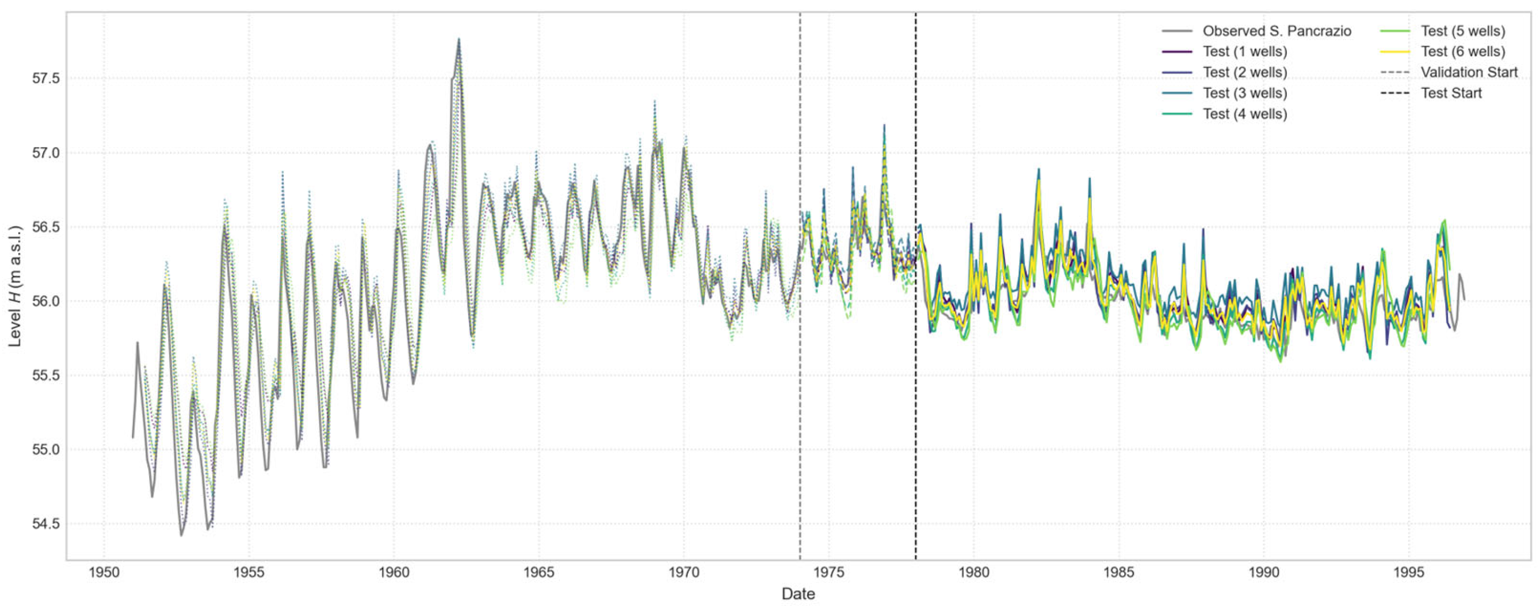
Figure 20.
Comparison of Open-Loop predictions for the “S. Pancrazio” well, with a 1-month forecast horizon. The plot illustrates the performance of a series of models, each trained using an increasing number of input wells, from one to six.
Figure 20.
Comparison of Open-Loop predictions for the “S. Pancrazio” well, with a 1-month forecast horizon. The plot illustrates the performance of a series of models, each trained using an increasing number of input wells, from one to six.
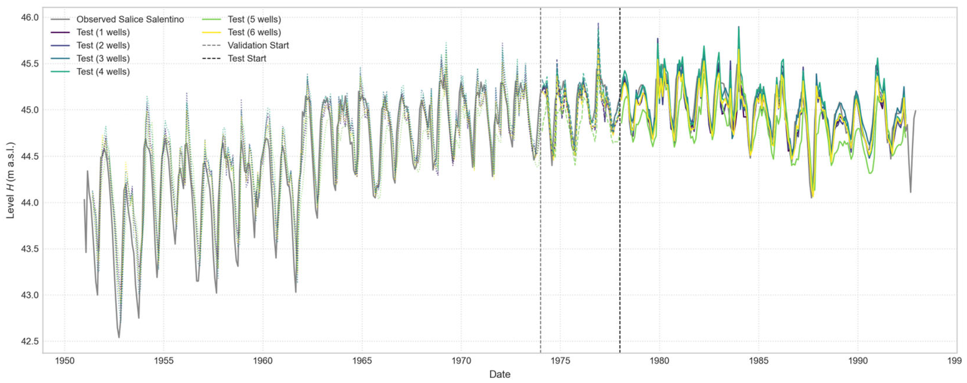
Figure 21.
Comparison of Open-Loop predictions for the Salice Salentino well, with a 1-month forecast horizon. The plot illustrates the performance of a series of models, each trained using an increasing number of input wells, from one to six.
Figure 21.
Comparison of Open-Loop predictions for the Salice Salentino well, with a 1-month forecast horizon. The plot illustrates the performance of a series of models, each trained using an increasing number of input wells, from one to six.
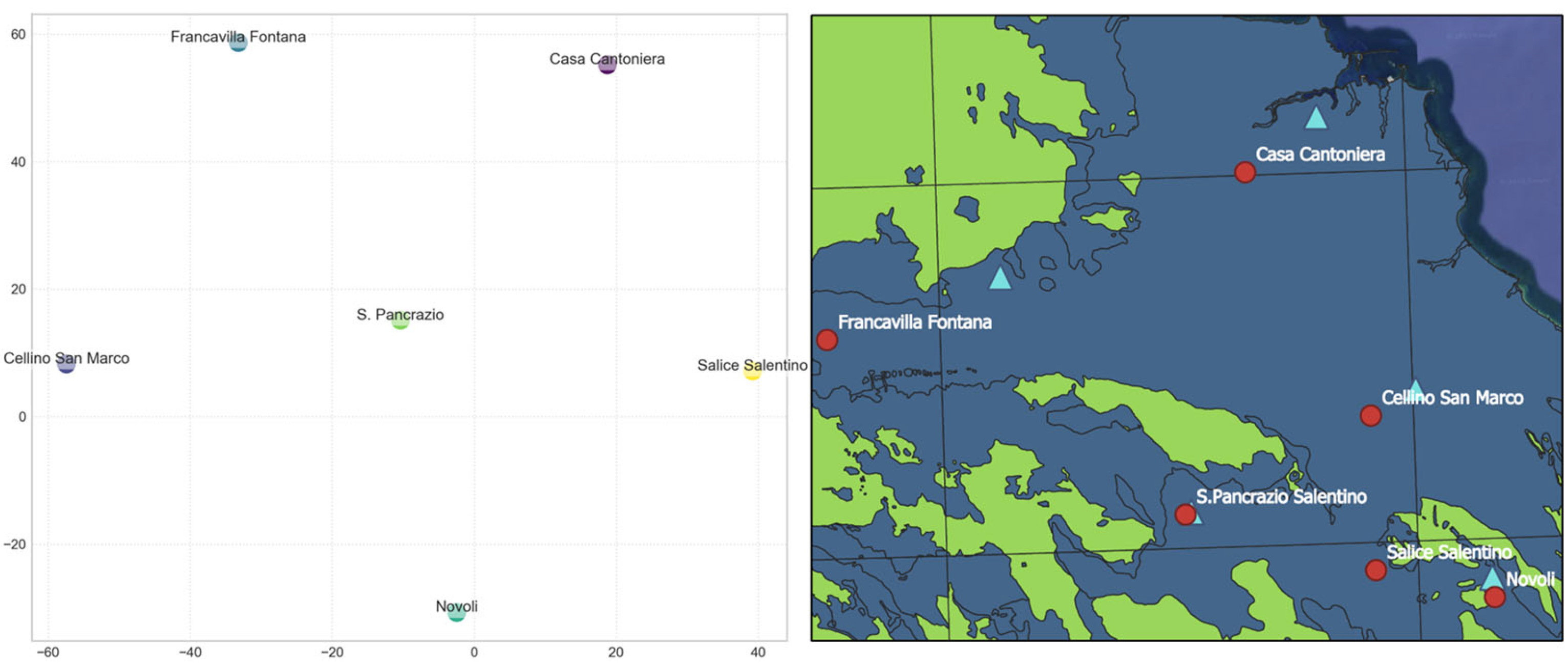
Figure 22.
Correlation between the positioning of the wells in the model’s learned embedding space (left) and their actual geographical layout (right), where in the right figure the red circles correspond to sampling wells, while cyan triangles represent rain gauge stations.
Figure 22.
Correlation between the positioning of the wells in the model’s learned embedding space (left) and their actual geographical layout (right), where in the right figure the red circles correspond to sampling wells, while cyan triangles represent rain gauge stations.
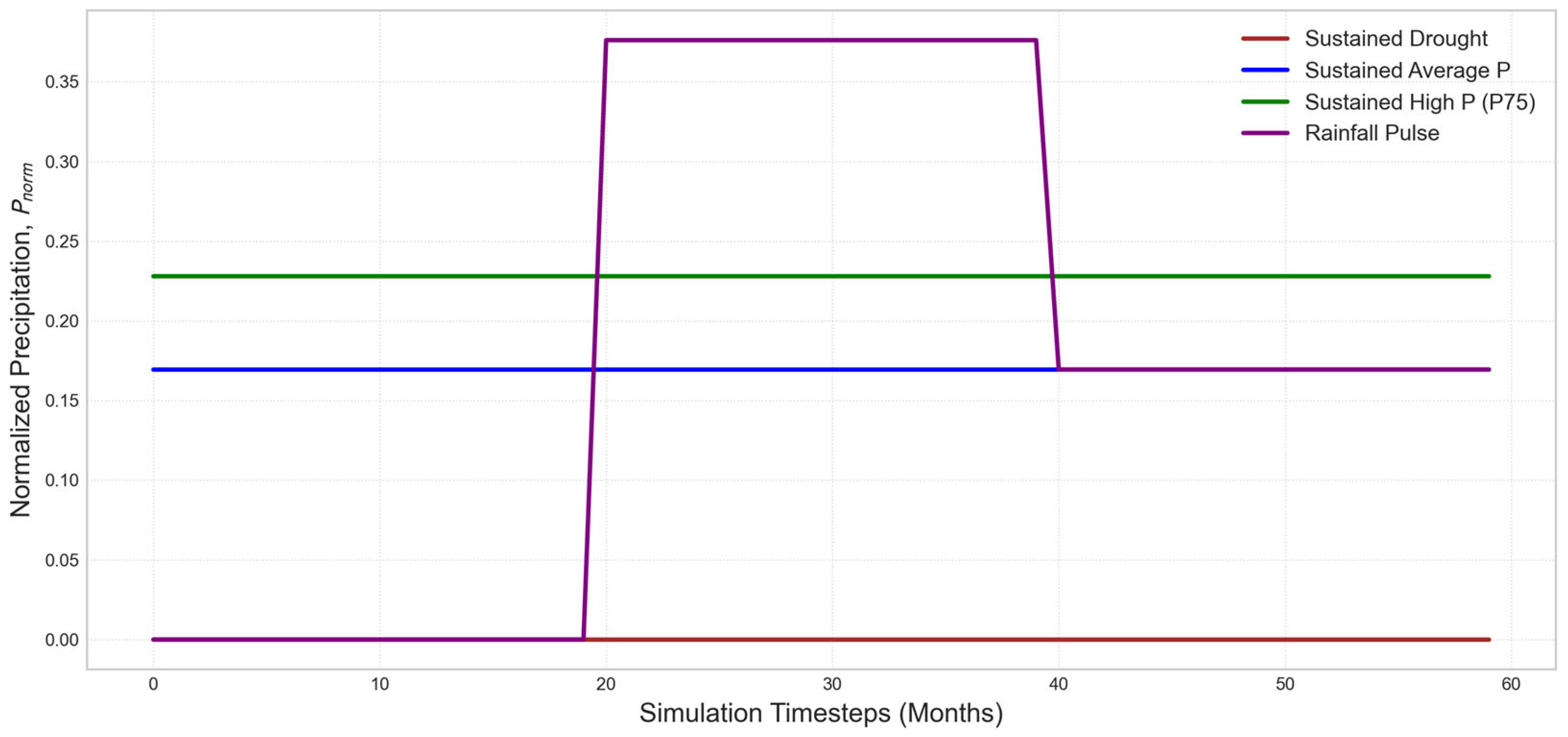
Figure 23.
Graphical representation of the four precipitation scenarios used for model simulations over a 60-month period. Each scenario is defined by a time series of normalized precipitation.
Figure 23.
Graphical representation of the four precipitation scenarios used for model simulations over a 60-month period. Each scenario is defined by a time series of normalized precipitation.
Figure 24.
Groundwater level projections for all six wells, comparing all scenarios. The plots show the predicted mean (solid lines) and uncertainty ranges (shaded areas) for each scenario.
Figure 24.
Groundwater level projections for all six wells, comparing all scenarios. The plots show the predicted mean (solid lines) and uncertainty ranges (shaded areas) for each scenario.
Table 1.
Details of the Investigated Wells.
Table 1.
Details of the Investigated Wells.
| Well Name | Date | Elevation (m a.m.s.l.) | Depth (m) |
|---|
| S. Pacrazio Salentino | 1951–1996 (45 years) | 58 | 2 |
| Casa Cantoniera | 1953–1996 (43 years) | 35 | 4 |
| Salice Salentino | 1951–1992 (41 years) | 46 | 1 |
| Cellino San Marco | 1951–1987 (36 years) | 57 | 6 |
| Novoli | 1962–1996 (34 years) | 35 | 11 |
| Francavilla Fontana | 1955–1982 (27 years) | 136 | 6 |
Table 2.
Summary of framework hyperparameters and configuration settings.
Table 2.
Summary of framework hyperparameters and configuration settings.
| Parameter | Value | Description |
|---|
| SEED | 32 | Seed for random number generators |
| WINDOW_SIZE | 5 | Number of past time steps (e.g., months) used as input |
| HORIZONS | (1, 2, 3) | Future prediction horizons (in time steps) for the model’s output during the open-loop phase |
| LSTM_UNITS | 46 | Number of units in the LSTM layer |
| LSTM_LAYERS | 1 | Number of LSTM layers in the core model |
| EMBEDDING_DIM | 4 | Size of the embedding vector for each well |
| EPOCHS | 150 | Maximum number of training epochs for each model |
| TEST_START_DATE | 1 January 1978 | Start date for the test set for all wells |
| VALIDATION_DURATION_YEARS | 4 | Duration of the validation set in years |
| ROLLING_FORECAST_HORIZONS | (1, 3, 7, 12) | List of horizons (L) to test in ‘Rolling Multi-Step Forecast’ mode during the closed-loop simulation |
Table 3.
Model σ mean for the entire test series. The table presents the forecasted standard deviation (σ) values one, two, and three months ahead, comparing Open-Loop simulation results for individual wells (“1 Well alone”) against models where the target well is supported by five additional wells (“1 Well supported by 5 Wells”).
| Well | σ 1 Month | σ 2 Months | σ 3 Months | σ 1 Months | σ 2 Months | σ 3 Months |
|---|
| | 1 Well Alone | 1 Well Supported by 5 Wells |
|---|
| Casa Cantoniera | 0.921731633 | 1.121058262 | 0.829408957 | 0.337532867 | 0.488939191 | 0.583101378 |
| Cellino San Marco | 2.861131741 | 3.147446002 | 3.115651124 | 0.685021842 | 1.022347641 | 1.240546083 |
| Francavilla Fontana | 1.165261519 | 1.194734437 | 0.816706758 | 0.191408214 | 0.271964254 | 0.347186325 |
| Novoli | 0.757368482 | 1.071530992 | 1.243149763 | 0.552066195 | 0.703314831 | 0.887721345 |
| S. Pancrazio | 0.224041011 | 0.348641935 | 0.422292953 | 0.291580448 | 0.398767864 | 0.506903108 |
| Salice Salentino | 0.229141452 | 0.364612261 | 0.430799924 | 0.259029697 | 0.36862028 | 0.487317109 |
Table 4.
Model performance evaluation, in Open-Loop simulation one month ahead, for individual wells (“1 Well alone”) versus models supported by five additional wells (“1 Well supported by 5 Wells”).
Table 4.
Model performance evaluation, in Open-Loop simulation one month ahead, for individual wells (“1 Well alone”) versus models supported by five additional wells (“1 Well supported by 5 Wells”).
| Well | MSE | MAE | R2 | MSE | MAE | R2 |
|---|
| | 1 Well Alone | 1 Well Supported by 5 Wells |
|---|
| Casa Cantoniera | 0.042076 | 0.187538 | −2.47802 | 0.000986 | 0.023351 | 0.918526 |
| Cellino San Marco | 0.0008 | 0.022094 | 0.608493 | 0.000701 | 0.018652 | 0.657276 |
| Francavilla Fontana | 0.041174 | 0.152356 | −0.60462 | 0.003043 | 0.038853 | 0.881425 |
| Novoli | 0.016188 | 0.100466 | 0.209543 | 0.009164 | 0.075448 | 0.552507 |
| S. Pancrazio | 0.001652 | 0.030518 | 0.344462 | 0.001866 | 0.031845 | 0.259462 |
| Salice Salentino | 0.003361 | 0.04218 | 0.637009 | 0.003012 | 0.041365 | 0.674698 |
Table 5.
Model performance evaluation, in forecast horizons L = 12 simulation, for individual wells (“1 Well alone”) versus models supported by five additional wells (“1 Well supported by 5 Wells”).
Table 5.
Model performance evaluation, in forecast horizons L = 12 simulation, for individual wells (“1 Well alone”) versus models supported by five additional wells (“1 Well supported by 5 Wells”).
| Well | MSE_L12 | MAE_L12 | R2_L12 | MSE_L12 | MAE_L12 | R2_L12 |
|---|
| | Model: 1 Well Alone | Model: 1 Well Supported by 5 Wells |
|---|
| Casa Cantoniera | 0.057432 | 0.217541 | −2.98651 | 0.007049 | 0.062549 | 0.510699 |
| Cellino San Marco | 0.002909 | 0.049205 | −0.35837 | 0.001124 | 0.025329 | 0.475057 |
| Francavilla Fontana | 0.054971 | 0.181728 | −1.25017 | 0.021883 | 0.090293 | 0.104233 |
| Novoli | 0.051709 | 0.199839 | −1.39868 | 0.049527 | 0.203103 | −1.29746 |
| S. Pancrazio | 0.009598 | 0.088073 | −2.80072 | 0.014196 | 0.105775 | −4.62163 |
| Salice Salentino | 0.017778 | 0.120302 | −0.8018 | 0.010472 | 0.089603 | −0.06136 |
Table 6.
Model performance evaluation, full Closed-Loop simulation, for individual wells (“1 Well alone”) versus models supported by five additional wells (“1 Well supported by 5 Wells”).
Table 6.
Model performance evaluation, full Closed-Loop simulation, for individual wells (“1 Well alone”) versus models supported by five additional wells (“1 Well supported by 5 Wells”).
| Well | MSE | MAE | R2 | MSE | MAE | R2 |
|---|
| | 1 Well Alone | 1 Well Supported by 5 Wells |
|---|
| Casa Cantoniera | 0.051167 | 0.20294 | −1.99272 | 0.013089 | 0.086262 | 0.234419 |
| Cellino San Marco | 0.014317 | 0.107462 | −3.60932 | 0.001108 | 0.025084 | 0.643265 |
| Francavilla Fontana | 0.067972 | 0.211615 | −1.46748 | 0.021038 | 0.100068 | 0.236299 |
| Novoli | 0.051417 | 0.193869 | −0.2211 | 0.05477 | 0.208617 | −0.30072 |
| S. Pancrazio | 0.010134 | 0.08682 | −1.40912 | 0.015588 | 0.110489 | −2.7058 |
| Salice Salentino | 0.02366 | 0.140252 | −1.57054 | 0.010815 | 0.090826 | −0.175 |


