A Review of Water Quality Forecasting and Classification Using Machine Learning Models and Statistical Analysis

Abstract

The prediction and management of water quality are critical to ensure sustainable water resources, particularly in regions like Malaysia, where rivers face increasing pollution from industrialisation, agriculture, and urban expansion. This review aims to provide a comprehensive analysis of machine learning (ML) models and statistical methods applied in forecasting and classification of water quality. A particular focus is given to hybrid models that integrate multiple approaches to improve predictive accuracy and robustness. This study also reviews water quality standards and highlights the environmental context that necessitates advanced predictive tools. Statistical techniques such as residual analysis, principal component analysis (PCA), and feature importance assessment are also explored to enhance model interpretability and reliability. Comparative tables of model performance, strengths, and limitations are presented alongside real-world applications. Despite recent advancements, challenges remain in data quality, model interpretability, and integration of spatio-temporal and fuzzy logic techniques. This review identifies key research gaps and proposes future directions for developing transparent, adaptive, and accurate models. The findings can also guide researchers and policymakers towards the development of smart water quality management systems that enhance decision-making and ecological sustainability.

1. Introduction

Water is a vital resource that sustains life, underpins ecosystems, and supports agricultural and industrial activities. Approximately 67.8% of the human body consists of water, making it indispensable for processes such as digestion, circulation, and temperature regulation [1]. Globally, 97% of the Earth’s water is saline, primarily found in oceans and seas [2]. While saline water is unsuitable for direct human use, it plays a crucial role in the global hydrological cycle. Ensuring access to clean and safe water is a cornerstone of public health. According to the World Health Organisation [3], 73% of the world’s population had access to safely managed drinking water services as of 2023. However, water pollution continues to pose a major environmental and public health threat. Industrial effluents, agricultural runoff, and untreated sewage contribute significantly to the degradation of water quality, affecting biodiversity and human livelihoods.

Global water scarcity is intensifying, affecting nearly 40% of the population, and this figure is expected to rise due to urbanisation, climate change, and population growth [4]. The United Nations projects that, by 2025, about 1.8 billion people will live in regions facing absolute water scarcity, while two-thirds of the global population will experience water stress [5]. Pollution-related impacts include reproductive issues in aquatic species due to heavy metals [6], as well as the formation of oxygen-deprived “dead zones” caused by nutrient overload [7]. Moreover, limited access to safe water, particularly in rural and low-income regions, exacerbates the spread of waterborne diseases such as cholera, dysentery, and hepatitis [8].

Although significant progress has been made in developing machine learning models for water quality prediction, most existing reviews focus either on global trends or generalised model performance. This research fills gaps in the literature on machine learning for water quality predictions. Its detailed presentation of statistical methodologies that support robust model construction makes this review different. This review is tailored to Malaysia’s environmental and regulatory framework. It analyses the National Water Quality Index (NWQI) and Department of Environment (DOE) guidelines that control local water management. This review addresses pollution issues resulting from industrialisation, agriculture, and urbanisation to make its findings and recommendations relevant to local researchers, policymakers, and environmental engineers. Then, this review goes beyond machine learning model comparisons. It includes a unique component on statistical analysis in water quality modelling. Other research may focus on predicting accuracy, but this review examines crucial validation techniques for model reliability and interpretability. This includes using residual analysis to evaluate model fit, diagnostic tests to verify assumptions, feature analysis to understand predictor influence, and principal component analysis (PCA) for dimensionality reduction. Statistical analysis gives readers a more holistic framework for creating, verifying, and evaluating water quality management machine learning models.

This review aims to

• Systematically categorise and compare machine learning and statistical models (including regression, classification, hybrid, and ensemble approaches) used in water quality prediction;
• Benchmark model performance using common evaluation metrics such as RMSE, R², accuracy, and F1-score to assess predictive capability;
• Assess the limitations, applicability, and interpretability of these models in the context of Malaysia’s environmental and regulatory requirements;
• Highlight statistical analysis techniques such as residual analysis and PCA that complement machine learning methods in model validation and optimisation;
• Identify current research gaps and propose future directions for the integration of artificial intelligence (AI) and data-driven decision-making in sustainable water quality management.

This review focuses on water quality forecasting and classification for surface water that consists of rivers and lakes. This review is organised into eight sections. Section 1 provides an introduction and the objectives of this review. Section 2 discusses the importance of water quality monitoring to justify why we have completed this review. Section 3 offers a detailed overview of water conditions and water quality standards since the monitoring method can be different for any country. Section 4 examines previous machine learning techniques applied in monitoring water quality, and this section becomes the main focus of this review. Section 5 is a continuation from Section 4, which explores ensemble methods used in developing hybrid models for enhanced forecasting and classification. Section 6 focuses on statistical methods in water quality management, where the previous studies are also compared. Statistical methods are important in analysing water quality to evaluate data tabulation and variation. Section 7 highlights the challenges and limitations of current studies that can assist future researchers in developing new water quality monitoring methods. Finally, Section 8 concludes this review.

2. Water Quality Monitoring

Advanced water quality monitoring is essential for managing environmental health and public safety. With the evolution of sensor technologies, environmental monitoring systems have become more precise, offering real-time data that enhance decision-making. Modern sensors can measure a wide range of physical (e.g., turbidity and temperature), chemical (e.g., pH and dissolved oxygen (DO)), and biological (e.g., pathogen presence) parameters [9,10]. In recent years, smart water quality monitoring systems have emerged by integrating Internet of Things (IoT) devices with artificial intelligence (AI). IoT-enabled sensors collect real-time water quality data, which are then analysed using AI algorithms to detect anomalies and trends [11]. Technologies such as smart buoys and wireless sensor networks have been effectively deployed for monitoring water quality in rivers, lakes, and coastal zones, particularly in large or remote areas where manual sampling is challenging [12,13]. However, their deployment is often constrained by factors such as sensor calibration drift, power supply limitations such as reliance on solar energy, latency in data transmission, and susceptibility to environmental interference. The integration of fuzzy logic into these systems helps manage the uncertainty and imprecision associated with real-time environmental data, enhancing interpretability and decision-making. Fuzzy logic-based decision-making mimics human reasoning and offers nuanced interpretations of water quality states, making it a valuable addition to automated monitoring frameworks [14].

Water quality classification is a critical aspect of environmental monitoring that transforms complex data into actionable categories. These classifications guide environmental policies, identify pollution sources, and aid in public health risk assessments. Traditional classification methods have evolved with the adoption of machine learning (ML) algorithms such as Naive Bayes and multilayer perceptron, which can accurately categorise water bodies based on parameters like pH, DO, turbidity, and ammoniacal nitrogen [15,16]. In addition to classification, forecasting plays a pivotal role in proactive water quality management. Regression techniques such as linear regression and ensemble methods like random forest have shown effectiveness in predicting water quality metrics based on historical data patterns. Random forest stands out for its ability to handle high-dimensional, non-linear datasets and is frequently used for both classification and regression in aquatic systems [17,18]. These approaches support more informed decision-making and help reduce the risk of pollution-related incidents.

3. Water Quality Conditions and Standards

3.1. Comparison of Water Quality Standards (WQSs) Globally

Water quality standards (WQSs) differ significantly across nations due to variations in ecological conditions, legal frameworks, and socio-economic priorities. While many countries align their water regulations with guidelines issued by the World Health Organisation (WHO), national adaptations are necessary to accommodate local environmental challenges [19,20]. For example, in the United States and Canada, WQSs are flexible and regionally adapted, focusing on chemical safety and risk management [21]. Canada has also tailored its standards to protect diverse ecosystems across its vast terrain. In contrast, the European Union enforces unified water directives across member states, promoting cross-border consistency in monitoring and certification processes [22]. In Asia, significant variability exists. Indonesia’s water quality is assessed using both the Pollution Index (PI) and WQI, which can yield conflicting interpretations of pollution severity [23].

Table 1. Comparison of water quality standards across various countries.

Country	Parameters Assessed	Clarification Levels
Global [24]	Drinking and surface water	Varies across regions
Indonesia [23]	PI and WQI	WQI shows “excellent”; PI indicates pollution
China [25]	Microbiological, fluoride, nitrate	89% compliance overall
India [26]	BOD, Total Coliform	High pollution in industrial zone
United States/Canada [24]	Drinking and surface water safety	Flexible, risk-based approach
Europe [27]	WQI, pollutant concentration	Excellent and poor class
Malaysia [28]	Six physicochemical parameters	Class I to V

compares key WQS elements across selected countries.

3.2. Water Conditions in Malaysia

Malaysia’s water supply is primarily derived from two sources: surface water and groundwater. Despite being a country rich in water resources, Malaysia faces increasing challenges to water quality due to rapid industrialisation, urbanisation, and population growth [29]. These developments have intensified environmental stress on rivers and catchments, exacerbated by the limited scope and prioritisation of water resource studies when compared to broader climate-related research [30]. The COVID-19 pandemic further impacted water quality, as lockdowns and the halting of non-essential services, including infrastructure and environmental monitoring projects, resulted in reduced oversight and maintenance [31]. Key contributors to river pollution include untreated domestic sewage, agricultural runoff, and discharges from manufacturing industries. Additionally, groundwater in proximity to agricultural zones, waste dumps, and radioactive landfills has shown elevated levels of arsenic, iron, lead, and other contaminants.

A colourimetric detection system for identifying metal ions in water has been developed to monitor contamination levels in real time [32]. Despite these innovations, recent government assessments highlight continued degradation. According to a report by the Department of Environment (DOE), 29 of 672 rivers across Malaysia were categorised as polluted [33]. In response, calls have been made for a dedicated water enforcement agency to oversee contamination control and regulatory compliance. Policy efforts have since intensified. The Ministry of Energy Transition and Water Transformation (PETRA) launched the Water Sector Transformation 2040 (WST 2040) initiative, which views water not just as a resource but as a strategic economic asset. The program emphasises improved water governance, investment in treatment infrastructure, and public awareness campaigns to ensure long-term water sustainability [34]. These developments reflect the country’s growing commitment to safeguarding both the ecological integrity and socio-economic value of its water systems.

3.3. The National Water Quality Index (NWQI) in Malaysia

The NWQI was established by the Department of Environment in Malaysia in 2020 with the objective of assessing and classifying the quality of surface water in Malaysia [28]. The framework known as the DOE-WQI is frequently cited as a set of standards [35,36,37]. The determination of local water quality and its characteristics was conducted in accordance with the national water quality requirements in Malaysia. The surface water quality and its classification were calculated by the MWQI model, which utilised six standard physicochemical water quality parameters: pH, ammoniacal nitrogen (AN), biochemical oxygen demand (BOD), chemical oxygen demand (COD), total suspended solid (TSS), and dissolved oxygen (DO). The parameters of the model were established through a collective agreement among experts, as shown in

Table 2. Parameters that are used in the NWQI [28,38].

Parameter	Unit	Class
		I	II	III	IV	V
AN	mg/L	<0.1	0.1–0.3	0.3–0.9	0.9–2.7	>2.7
BOD	mg/L	<1	1–3	3–6	6–12	>12
COD	mg/L	<10	10–25	25–50	50–100	>100
DO	mg/L	>7	5–7	3–5	1–3	<1
pH	-	>7.0	6.0–7.0	5.0–6.0	<5.0	>5.0
TSS	mg/L	<25	25–50	50–150	150–300	>300
WQI		>92.7	76.5–92.7	51.9–76.5	31.0–51.9	<31.0

[35].

The categorisation system categorises water into five types based on certain essential quality factors. AN serves as a crucial parameter for identifying pollution, mainly originating from waste sources. Class I denotes levels below 0.1 mg/L, indicating minimal contamination and making it appropriate for delicate aquatic ecosystems. On the other hand, Class V is above the threshold of 2.7 mg/L, which indicates a substantial level of contamination. BOD is an indicator of the amount of organic pollution present in water. In Class I, the BOD is below 1 mg/L, indicating that the water is exceptionally clean. Nevertheless, Classes IV and V exhibit BOD values exceeding 6 mg/L and 12 mg/L, respectively, which suggest elevated quantities of organic waste and diminished water quality.

COD is a measure of the overall quantity of chemicals that can be oxidised. Class I, which has a COD of less than 10 mg/L, indicates a low presence of chemical pollutants. On the other hand, Class V, with a COD above 100 mg/L, indicates a high level of pollution. The levels of DO are vital for the survival of aquatic species. A minimum of 7 mg/L of COD in Class I is necessary to maintain a thriving aquatic ecosystem, whereas less than 1 mg/L of COD in Class V is inadequate to support the health of aquatic animals. The pH level is a crucial element. Class I water maintains a neutral to slightly basic environment with a pH level of more than 7.0, which is ideal for most aquatic life. On the other hand, Class IV and V water has very acidic or alkaline pH levels, which can harm aquatic creatures. The measurement of TSS is used to determine the clarity of water. Class I water has TSS levels below 25 mg/L, indicating clear water. On the other hand, Class V water has TSS levels exceeding 300 mg/L, which indicates high turbidity and significant ecological problems.

The pH is an important water quality parameter to determine the basicity of an aqueous solution. A pH value from 0 to 14 indicates the acidity, neutrality, or alkalinity of the water [39]. An acidic solution has a pH less than 7, and pH~7 indicates a neutral solution. Meanwhile, a pH greater than 7 indicates an alkaline solution. Unreasonably high or low pH of water is not safe for household usage and drinking water [40]. The acceptable pH for consuming and drinking water is from 6.5 to 9 [41]. The measurement of dissolved oxygen (DO) serves as a significant metric for assessing the overall well-being of an aquatic ecosystem. The presence of DO is crucial for the viability of many aquatic creatures since inadequate levels of dissolved oxygen can result in fish mortality and other associated complications.

According to the authors of [42,43], the COD of water is an important indicator of water quality. This metric measures the amount of oxygen required to break down contaminants; hence, it can be a good indicator of the water pollution load. In general, it is recommended to maintain low COD levels for natural waters and effluents that are released into aquatic habitats. Excellent quality, organically uncontaminated natural waters are defined as having a COD value below 50 mg/L. Modestly polluted streams, commonly found in metropolitan areas or due to agricultural runoff, typically have values between 50 and 100 mg/L.

The BOD is a critical measure of the extent to which liquids are polluted with organic substances [44]. The oxygen consumption rate of aerobic bacteria is measured over a set length of time, usually five days at 20 °C, in order to determine the amount of organic debris in water. After standard treatment and disinfection, water is fit for human consumption if its BOD level is less than 3 mg/L, which is a great indicator of purity. Moderately affected bodies of water often have levels between 3 and 6 mg/L, which means that they may need extra treatment before they can be consumed by humans [45].

The TSS concentration is an important metric for water quality assessment. Small particles that cannot settle to the bottom of the water column can cause a cloud to form, which in turn affects aquatic life by making food less accessible and making it harder for aquatic plants to produce oxygen through photosynthesis [46]. An important metric for water quality is AN, abbreviated as NH3-N. Ammonia is a kind of nitrogen that is produced during organic matter breakdown and is a byproduct of wastewater discharge. While there is no universally accepted limit for ammoniacal nitrogen in freshwater systems, it is typically recommended that the level be kept below 0.02 mg/L in order to safeguard aquatic life.

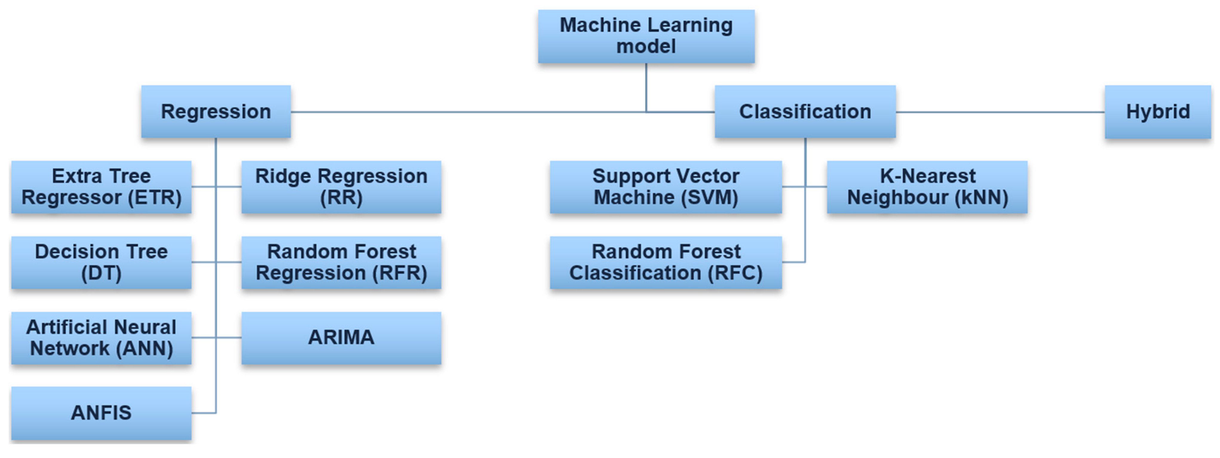
4. Machine Learning Models for Water Quality Forecasting and Classification

4.1. Forecasting-Based Water Quality Management

Forecasting water quality plays a pivotal role in environmental management, enabling proactive interventions to mitigate pollution and preserve aquatic ecosystems. In recent years, both classification and regression-based ML models have been widely adopted for this purpose, owing to their ability to model complex, non-linear interactions among environmental variables [47]. Accurate forecasts not only ensure the availability of clean water for domestic and industrial use but also support biodiversity protection and fisheries management. Traditional methods often fall short by neglecting the influence of diverse factors such as chemical reactions, hydrological processes, and biological dynamics. As a result, advanced techniques, such as artificial neural networks (ANNs), random forests (RFs), Extreme Gradient Boosting (XGBoost), Autoregressive Integrated Moving Average (ARIMA), K-Nearest Neighbours (KNNs), and fuzzy systems, have been proposed to enhance water quality prediction [48].

Several studies highlight the successful application of advanced modelling techniques for water quality prediction. For instance, long short-term memory (LSTM) networks provided high-precision forecasts, although their reliability varied between different river basins [49]. ANNs were also effective in assessing and simulating water quality changes in geographically distinct rivers [50]. In a similar vein, a novel deep learning model known as LTSF-Linear enhanced prediction accuracy in a reservoir case study by better handling complex data patterns [51]. Furthermore, a hybrid VMD-GWO-GRU model significantly outperformed standalone models, especially for longer-term predictions, by improving how the data signal was decomposed [52].

The application of machine learning extends to real-time monitoring and leveraging diverse data sources. One study effectively used AI with Sentinel-2 satellite imagery to forecast coastal water quality, finding that different models like SVMs and ARIMA were better suited for specific parameters [53]. For modelling dissolved oxygen, a Bayesian-Optimised SVR model proved superior and helped identify the most influential environmental factors [54]. Another paper showcased a highly accurate (99.8%) ensemble machine learning model integrated into an autonomous IoT and cloud-based system for real-time water quality monitoring and prediction [55].

Despite these advancements, the studies share common limitations. A primary concern is the dependency on data quality; one study noted issues with missing data and outliers [51], while the accuracy of another depended heavily on the initial field measurements [50]. The scope of these models can also be narrow. For example, research was sometimes limited by a small number of water quality parameters or a small dataset [52,55]. Finally, specific models had their own inherent weaknesses, such as sensitivity to parameter selection [52] or a lack of understanding behind performance variability [49].

The WQI is commonly used as a forecasting target. The WQI quantifies the status of water quality based on core physicochemical parameters, with higher values indicating better water conditions [56]. Classification frameworks derived from WQI scores categorise water as safe, mildly polluted, or highly contaminated [57]. However, manual calculation of the WQI is time-consuming and prone to errors, reinforcing the need for automated, data-driven forecasting systems.

Table 3. Previous studies on machine learning methods for water quality management.

Ref.	Modelling Techniques	Advantages	Disadvantages	Data Size	Water Parameters
[49]	Long Short-Term Memory (LSTM)	High accuracy in predicting water quality indicators across multiple basins.	Model tuning details are limited, reducing reproducibility.	Dataset size is not stated but covers three rivers.	AN, BOD, COD, DO, pH, and total phosphorus (TP).
[50]	Artificial Neural Networks (ANNs)	Employs a novel Absorption Characteristics Recognition (ACR) algorithm, delivering optimal regression performance.	The ACR method lacks detailed performance benchmarks regarding computational cost and robustness.	200 spectral readings.	TP, COD, turbidity, total nitrogen (TN), chlorophyll.
[53]	AI-driven Time Series (SVM and ARIMA) with Satellite Imagery	The hybrid framework combining Sentinel-2 imagery with SVM and ARIMA models increased spatial data coverage.	ARIMA is less optimal for non-seasonal parameters; limited subsurface insight.	Dataset size is not stated.	Chlorophyll, Secchi Depth, Trophic State Index.
[51]	Deep Learning (LTSF-Linear Model)	Linear model baseline outperformed ARIMA, LSTM, and Informer, reducing MSE and MAE by 8.55% and 10.51%.	Limited to three parameters, restricting applicability to more complex multi-parameter models.	Hourly measurements from January 2022 to July 2023	pH, turbidity, DO.
[58]	Proposed chlorine level assessment using IoT system and machine learning.	The random forest model achieved high accuracy with an F1-score of 0.89 for chlorine level classification.	Lacks comparison with more diverse models.	Dataset size is not stated.	Residual chlorine.
[59]	Proposed mass balance model to monitor the water quality at the river.	Provides a robust benchmark with 18,000 scenarios across varied network types.	Limited to chlorine dynamics; not evaluated for other water quality parameters.	18,000 simulation cases.	Chlorine concentration.
[60]	Case study on the effect of lockdown period on surface water pollution and quality.	Uses advanced AI (deep learning, ensemble) to directly predict WQI and water quality classes.	Details on data volume and parameter list are not fully disclosed.	33,612 samples.	BOD, COD, DO, turbidity, heavy metals (e.g., Pb, Zn).
[61]	Predicted the BOD using data from New York Harbor waters.	RMSE was 11.5–17.2% lower than regular matrix-completion approaches and 19.2–25.2% lower than classic machine learning models.	Deep models require extensive data to perform well.	32,323 samples.	BOD, pH, DO, temperature.
[62]	Predicted DO concentration using different water quality parameters.	Best hybrid reduces RMSE by 80% from standalone MLP.	A small dataset size may limit broad applicability.	232 samples.	Chlorine, TDS, pH, temperature.
[63]	Proposed water quality classification using Landsat8 images by CNN.	CNN provided superior classification over traditional ML approaches.	Temporal mismatch between satellite capture and sampling, plus weather variability.	481 samples.	DO, TN, TP, COD and Ammonium
[64]	Proposed the assessment of heavy-metal pollution in water to detect Pb, Cu, and Zn.	CNNs showed strong potential in mapping chlorophyll-a concentration from satellite data.	Deep learning models perform best with large, labelled datasets.	Dataset size is not stated.	Chlorophyll.
[65]	Proposed prediction river WQI for river pollution prevention and management. Algorithm comparison with PSO, GA, LSTM, and SVM.	Hybrid adaptive evolutionary artificial bee colony–backpropagation neural network (AEABC–BPNN) searches more reliably for global optima.	Combining evolutionary algorithms with neural networks adds architectural and training complexity.	Dataset size is not stated.	pH, turbidity, nutrients.
[44]	Prediction of biochemical oxygen demand with GA-based SVR to ensure the quality of water.	SVR optimised via genetic algorithm (GA) outperformed linear regression and MLP, indicating effective feature-selection and parameter tuning.	Reliance on past data and GA tuning might restrict generalizability to new water bodies.	Dataset size is not stated.	AN, TP, TN, pH, DO, COD.
[66]	Proposed dissolved oxygen prediction at rivers using PCA, LSSVM, and improve PSO.	Best model (Gradient Boost) scored R2 ≈ 1.00 and MAE ≈ 0.08, robust across two WWTP datasets.	While tested across two plants, many models may need recalibration for other regions.	Dataset size is not stated.	Flow rate, COD, pH, AN, TSS.
[67]	Proposed water quality prediction model by using ARIMA, LSTM, GRU, and SCINet algorithms.	Utilises state-of-the-art deep learning to model complex temporal patterns.	Limited parameter scope: only three water quality indicators excluding others like microbial or chemical contaminants.	47,448 samples.	pH, turbidity, residual chloride.
[68]	Study assessment and prediction of water quality index using fuzzy logic and ANN models.	Hybrid modelling approach combines fuzzy logic with ANNs, blending interpretability and adaptive prediction.	Dataset specifics unclear, making it difficult to evaluate robustness or representativeness.	Dataset size is not stated.	pH, DO, TSS, nutrients.
[69]	Proposed water quality indicator prediction for wastewater using improve Bald Eagle Search and least-square support vector machine.	Goes beyond point estimates, providing ranges for BOD and AN, enhancing operational safety and risk assessment.	Designed for wastewater effluent; may not generalise to other water systems without recalibration.	Dataset size is not stated.	BOD, AN.

shows various previous studies on the application of machine learning techniques for water quality management. All techniques are reviewed in terms of advantages and disadvantages, data size, and water quality parameters that have been studied.

The emphasis area is shown in Figure 1, which also includes a list of machine learning models for classification, regression, and a hybrid model.

4.2. Regression-Based Prediction Models

Regression methods estimate continuous water quality parameters by learning patterns from historical data. Notable approaches include the following:

4.2.1. Extra Tree Regressor (ETR)

An ensemble learning method known as Extra Tree Regressor (ETR) constructs several DTs using randomised split points. This approach can reduce variance and enhance accuracy when dealing with complex environmental datasets. This model shows strong effectiveness in situations involving high-dimensional data and non-linear patterns, as it averages predictions across many trees to enhance stability [70]. A study demonstrated the effectiveness of ETR in predicting water quality, achieving strong results across different environmental parameters [71]. Another article employed ETR to predict turbidity levels in drinking water treatment facilities, demonstrating that this model can effectively handle the dynamic, non-linear interactions between meteorological and water quality data [72]. The model showed strong performance in predictive accuracy, to improve treatment processes based on environmental inputs. Because of the significant randomness and the numerous trees involved, Extra Trees might be harder to interpret in comparison with individual DTs.

4.2.2. Ridge Regression (RR)

Ridge Regression (RR) is a technique that reduces overfitting by incorporating a penalty for large coefficients. This method is useful for environmental applications where predictors show multicollinearity. This method is used to predict sulphate concentrations in acid mine drainage, where multicollinearity among water chemistry indicators often occurs [73]. RR provided a reliable solution that handled correlated features well, improving the model’s predictive accuracy and making it appropriate for ongoing monitoring of sulphate levels in water bodies affected by mining. A different study utilised RR in a spatial-temporal analysis of coastal water salinity, effectively modelling salinity levels by considering interacting environmental variables such as temperature and dissolved salts [74]. The regularisation of the model contributed to the development of accurate and stable predictions, avoiding the overemphasis on any single factor, which is crucial in complex, multi-parameter coastal systems. RR keeps all predictors, but the penalty can complicate understanding the precise impact of each predictor, since coefficients tend to be biased towards zero.

4.2.3. Decision Tree (DT)

Decision tree (DT) is an intuitive and widely used model for both classification and regression tasks, particularly suitable for data where relationships are non-linear or threshold-based. DT proves to be particularly beneficial in exploratory analysis or in situations where clarity is essential. The DT was used to predict water quality indicators in Malaysia’s Kereh River, comparing its effectiveness with other models and showing how well it captured river conditions based on factors such as turbidity and dissolved oxygen [75]. Another study also utilised DT to evaluate and forecast water quality levels through a WQI, demonstrating that the model successfully classified and quantified quality levels based on environmental parameters [76]. The next decision tree was used to predict the water quality index of groundwater in Mirpurkhas, Pakistan [77]. Some applications showcase the model’s ability to handle intricate, threshold-based water quality data. DT models are utilised to predict changes in surface water quality across various seasons, demonstrating their adaptability in forecasting dynamic water conditions for environmental management [78]. DT models are effective tools for doing classification and regression tasks [79]. This study examined the application of DT in predicting water quality, highlighting its efficacy in modelling intricate environmental data. DT is suitable for non-linear and threshold-based relationships, which makes it effective in environmental contexts where variables interact in complex ways. However, it can be prone to overfitting, particularly when the tree becomes deep and complex.

4.2.4. Random Forest Regression (RFR)

Random forest regression (RFR) is a strong ensemble method that constructs several decision trees and averages their predictions. This approach helps in reducing overfitting and achieving high accuracy for non-linear data. Its application in water-related predictions has demonstrated impressive results. This study utilised RFR to improve WQI and Positive Matrix Factorisation (PMF) models, enhancing their accuracy in predicting water quality by managing complex data relationships [80]. This integration could result in new insights and advancements in understanding the dynamics of water quality and the sources of pollution. This study showed that random forest regression was effective in precisely predicting important water quality indicators such as salinity, pH, dissolved oxygen, and temperature in aquaculture environments [81]. A different study showed that RF was very accurate in predicting groundwater quality, surpassing other models such as SVMs and DTs [77]. The regression trees produced by RFR exhibit a low bias and a high variance profile. The reliability of RF in managing complex environmental data makes it particularly well suited for accurate water quality assessments. Averaging multiple trees leads to high accuracy and stability, which makes RF regression a good choice for complex datasets that might challenge single models. RF regression relies on large datasets to promote diversity among trees, which means that small datasets can restrict its effectiveness.

4.2.5. Artificial Neural Networks (ANNs)

Artificial neural networks (ANNs) are highly effective tools for accurately representing intricate and non-linear connections across extensive datasets, which makes them well suited for implementing aquatic smart decision systems. ANN models are utilised for the prediction of water quality indices, showcasing their efficacy in capturing intricate data patterns [82]. The utilisation of ANNs for predicting water parameters in smart aquaculture was mostly centred around the implementation of random forest models [81]. In addition to evaluating the influence of treated effluent on water quality, an ANN demonstrated its usefulness in environmental assessments [83]. An ANN was employed to simulate the water quality index of the Air Busuk River based on chemical factors [84].

4.2.6. Autoregressive Integrated Moving Average (ARIMA)

Autoregressive Integrated Moving Average (ARIMA) is a widely used time series model that is suitable for predicting environmental data with seasonal trends. A time series refers to a collection of data points that are recorded and arranged in chronological order. Time series analysis encompasses the observation and study of temporal data, with the aim of identifying patterns of change and development, as well as making predictions about future trends. Hasnan et. al [85] introduced an ARIMA and clustering model to predict water quality in a river basin. The ARIMA model is a commonly employed technique for modelling time series data. The ARIMA modelling technique was employed by [86] to facilitate predictive maintenance for the smart toilet, and its performance was subsequently compared to the LSTM model. The model has a strong fit to the data and exhibits minimal prediction error. A different study employs ARIMA and Transfer Function ARIMA (TFARIMA) models to examine water quality parameters such as turbidity, colour, and iron in a drinking water supply system located in Bogota, Colombia [87]. This analysis encompasses the system’s river, reservoir, and treatment plant. TFARIMA shows that there is a limited direct influence between water sources, which aids in identifying and managing temporary or persistent water quality issues. ARIMA is effective for analysing single-variable time series, like temperature or turbidity in a specific water source, where the past values of one parameter can forecast its future states.

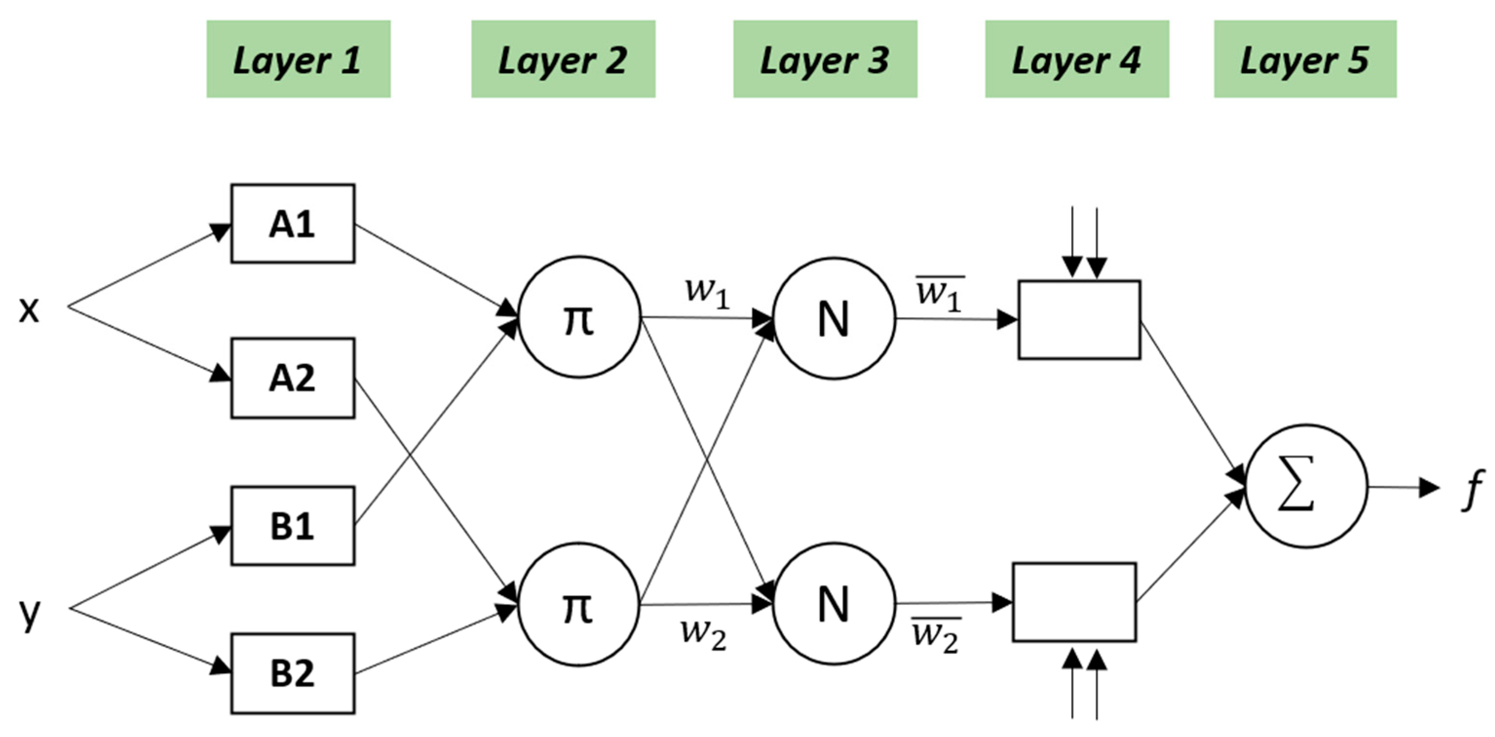
4.2.7. Adaptive Neuro-Fuzzy Inference System (ANFIS)

Article [88] asserts that the Adaptive Neuro-Fuzzy Inference System (ANFIS) is an effective water decision-making system tool due to its utilisation of fuzzy logic to deal with ambiguous and imprecise data and neural networks for learning. Recent studies have utilised ANFIS for various water prediction purposes, demonstrating its adaptability in domains tangentially linked to environmental science and water management. ANFIS serves as a predictive tool for optimising wastewater reuse in agriculture, ensuring the maintenance of water quality, as illustrated in Figure 2 [89]. Layer 1 utilises fuzzy membership functions to evaluate the inputs ($x$ and $y$) and ascertain their degree of membership within the fuzzy sets (A1, A2, B1, and B2). Layer 2 calculates the firing strengths ($\pi$) of each fuzzy rule by multiplying the input membership degrees. In Layer 3, the firing strengths are normalised ($N$) to establish relativity across rules. Layer 4 computes the weighted outputs ($\overline{w_1}{f}_1$, $\overline{w_2}{f}_2$) through the application of normalised firing strengths to functions that are specific to each rule. Layer 5 aggregates the weighted outputs ($\Sigma$) to yield the final classification result ($f$).

4.3. Classification-Based Prediction Models

Classification methods in machine learning categorise data into predefined classes or groups, which are essential for predictive analytics in various domains. These methods work by analysing labelled training data and subsequently predicting the class label of new, unseen data according to the patterns that have been learnt. These models classify water quality into predetermined categories, such as “safe” or “unsafe”. Classification entails utilising past water quality data to train the algorithm to identify trends and make categorical forecasts regarding new data. The authors of [90] employed logistic regression in conjunction with principal component regression to categorise water quality, emphasising its usefulness in the field of environmental science. The simplicity and efficacy of logistic regression make it a great tool for analysing correlations between variables in classifying water quality.

4.3.1. Support Vector Machines (SVMs)

Support vector machines (SVMs) are robust supervised learning models for regression and classification methods. SVMs can classify data or predict continuous values by identifying the hyperplane that achieves this most effectively. Ultra-precision machining uses SVMs to forecast surface roughness, proving the technology’s usefulness in environmental data modelling [91]. Sufficient capacity to deal with complicated and high-dimensional data makes SVMs a good choice to obtain precise results. Predicting and classifying river water quality using SVMs demonstrates their efficacy in dealing with various datasets [92]. The classification capabilities of SVMs enabled the precise parameter-based categorisation of water quality measures. The accuracy and stability of the hybrid water quality prediction model were enhanced by integrating SVMs with other approaches [93]. The model improved its predictive abilities by integrating SVMs with Wavelet decomposition and GRU, among other techniques. Article [94] found that an SVM was a useful technique for incorporating remote sensing data into water quality predictions due to its capacity to manage big and complicated datasets. Article [95] showed that an SVM achieved superior performance compared to other models, such as decision trees and ANNs, in the prediction of river water quality. The method highlights the effectiveness of SVMs as a tool for classifying environmental data. Logistic regression is a statistical technique used for binary classification. It predicts the likelihood of a binary result by considering one or more predictor factors.

4.3.2. K-Nearest Neighbours (KNNs)

K-nearest neighbour (KNN) is a straightforward and non-parametric technique employed for classification. It involves determining the k-nearest data points to a particular query point and making predictions based on the values of these neighbouring points. In their study, the authors of [96] suggested a hybrid classification model that integrates KNN with PCA and voting classification algorithms to enhance the accuracy of water quality prediction. The simplicity and efficacy of KNN in capturing local data patterns make it an excellent tool for environmental monitoring. KNN was utilised for classifying water samples according to the WQI, showing its effectiveness in distinguishing between categories such as “safe” and “unsafe” for consumption [76]. KNN may not have reached the highest accuracy in comparison with random forest, but it offers dependable classification in a simple and understandable way. A different study applied KNN in a water quality monitoring system using IoT, classifying water samples as either polluted or clean, based on sensor data [97]. The model reached an accuracy of 94%, showing that it was suitable for real-time applications with continuous data streams. KNN was used to classify groundwater quality based on physicochemical properties, showing that KNN can accurately categorise the data into quality levels, even though its performance was slightly lower than SVMs in terms of accuracy [98]. The model effectively adapts to non-linear boundaries in environmental data, making it suitable for complex, multi-parameter groundwater datasets. KNN stores the entire dataset and computes distances for every prediction, making it computationally expensive, particularly with large datasets or high-dimensional data. KNN tends to be less efficient when dealing with large-scale water quality databases or streaming data.

4.3.3. Random Forest Classification (RFC)

Random Forest Classification (RFC) depends on several decision trees, with each tree trained on a unique bootstrapped sample of the dataset. The capability of RFC to manage high-dimensional data and model non-linear relationships is particularly useful in situations where many features influence classification results. The RF classification algorithm is employed to forecast water quality after desalination, proficiently managing variables such as pH, hardness, and solids [99]. The method’s capacity to manage extensive datasets with a high number of dimensions makes it valuable for environmental applications. RFC is employed to classify water quality in surface water bodies utilising satellite imagery [100]. The model rated regions as safe or dangerous by spectral data analysis, with 94% accuracy and surpassing other models (KNN, SVM, DT, and NB) in distant water quality monitoring. A different study showed how RFC can effectively predict river water quality by integrating various water quality indicators [92]. This study demonstrates that RFC effectively manages various features, including turbidity, pH, and dissolved oxygen, resulting in precise classifications throughout different sections of the river. The ensemble method of RFC produces high accuracy because the combined output from multiple trees is less affected by the errors of individual models, which helps to reduce overfitting and enhances generalisability.

4.4. Hybrid Machine Learning Models

The objective of hybrid machine learning models in water quality prediction is to improve accuracy and provide a more comprehensive analysis by integrating multiple algorithms that serve different functions. These models combine the strengths of various techniques, such as using one model for capturing trends and another for classifying categories, to better manage the complexity of environmental data. For instance, a combination of artificial neural networks (ANNs) for regression and random forests for classification has been applied to predict solar power generation [101]. This integration addresses the unpredictability of solar energy, which is often influenced by changing weather conditions [102]. Similarly, other researchers have used ARIMA for capturing time-dependent trends and paired it with support vector machines and random forests for classification tasks [103]. This combination allows the model to capture both linear temporal patterns and complex categorical distinctions, offering more robust forecasting in dynamic systems.

A different study explored the use of a hybrid deep learning model that incorporates ensemble learning with randomised low-rank approximation to improve both prediction and classification of water quality [104]. By combining dimensionality reduction techniques with ensemble strategies, the model enhances both precision and generalisation. An innovative model integrates artificial neural networks with evolutionary polynomial regression to improve the prediction of water quality in distribution networks, particularly for Bogota’s municipal water system [105]. This approach helps improve both the reliability and interpretability of the results in urban-scale applications. Another proposed method, known as AEABC-BPNN, combines an artificial bee colony optimisation technique with a backpropagation neural network to predict the water quality index [65]. This study shows that this hybrid model converges in just 14 iterations and performs better than other models such as support vector machines, genetic algorithms, and long short-term memory networks.

In another example, researchers proposed an IPSO-LSSVM model that uses improved particle swarm optimisation and a least-square support vector machine to estimate dissolved oxygen levels in the Yangtze River in Shanghai [106]. This data-driven model benefits from the optimisation algorithm’s ability to fine-tune parameters, improving regression accuracy for environmental prediction. A common theme across these studies is the use of hybrid structures to manage both regression and classification tasks, which are often required in water quality systems where both continuous values and categorical risk levels must be interpreted simultaneously. The flexibility of hybrid models makes them suitable for complex environmental applications where accurate prediction, interpretability, and adaptability to changing conditions are all critical.

However, the process of fine-tuning multiple parameters across different algorithms remains a challenge. It often requires specialised knowledge and increased computational resources. Despite this, hybrid models offer valuable contributions to sustainable water management and public health monitoring by improving the reliability of data-driven decision-making.

4.5. Model Benchmarking and Comparative Performance Evaluation

This part gives a structured benchmarking of both regression and classification models using metrics that are consistent and interpretable. The purpose of this section is to provide a rigorous and transparent evaluation of the performance of the model. RMSE, MAE, and R² are the metrics that are utilised in the evaluation of regression models, whereas accuracy, precision, recall, and F1-score are utilised in the evaluation of classification models. The overall performance evaluation is shown in

Table 4. Performance benchmarking of regression models.

Model	RMSE	MAE	R2
ETR [66]	1.55	0.69	0.99
RR [107]	0.05	0.04	0.96
DT [66]	2.76	1.19	0.97
RFR [66]	1.71	0.74	0.99
ANN [108]	0.08	0.06	0.98
ANFIS [109]	0.14	0.09	0.97
ARIMA [110]	301.99	220.14	-

and

Table 5. Performance benchmarking of classification models.

Model	Accuracy	Precision	Recall	F1-Score
RFC [111]	98.2	0.98	0.98	0.98
KNN [112]	97.4	0.97	0.98	0.97
SVM [111]	97.9	0.98	0.98	0.98

. This standardised technique makes it possible to do a comparison of the capabilities and limitations of the model that is more useful. The benchmarking not only includes the reporting of performance statistics, but it also emphasises how each model behaves under a variety of different scenarios. For example, neural-based models (ANNs and ANFIS) and ensemble trees (ETR and RFR) regularly perform well in regression tasks, with high R² values and low error rates. These models can continuously achieve excellent performance. The Random Forest Classifier is the one that displays the finest overall balance across all measures when it comes to classification. In contrast, the ARIMA statistical method, which is a classic approach, has significantly greater error levels, which indicates that it is not suitable for highly dynamic or non-linear data. The readers will have a better understanding of which models are most suitable for achieving particular predicted goals in water quality monitoring if they align all of the models under a consistent evaluation framework with one another.

Based on the findings, it appears that ensemble methods and hybrid neural approaches are more robust when applied to a wide variety of circumstances. In the field of water quality forecasting, for instance, the Extra Tree Regressor (ETR) and the Random Forest Regressor (RFR) demonstrate high levels of predictive consistency and low levels of error. Ridge Regression (RR), on the other hand, provides a very low error rate for more straightforward linear trends. RFC achieves the highest overall accuracy in classification tasks; however, KNNs and SVMs also exhibit strong performance depending on the feature space and sample size. RFC is the most accurate classification method. The significance of these characteristics lies in the fact that it is essential to select models not just on the basis of their overall accuracy but also on the specific nature of the prediction task at hand, such as whether the objective is to forecast trends, identify outliers, or classify risks.

4.6. Small-Scale Implementation Using Malaysian Water Quality Data

To demonstrate the practical application of selected models in a Malaysian context, a small-scale implementation was conducted using a synthetically generated dataset based on the DOE WQI classification guidelines (as shown in Table 2). The dataset includes 50 samples of water quality readings constructed to reflect realistic environmental conditions across the five WQI classes. The six DOE standard parameters include pH, DO, BOD, COD, TSS, and ammoniacal nitrogen and are used as input features. The objective is to predict both WQI values (regression) and classify them into water quality classes (classification). Regression models such as Random Forest Regressor and ANNs achieve R² scores of 0.97 and 0.96, respectively, with low RMSE values. For classification, the Random Forest Classifier shows 96.7% accuracy, followed by KNNs and SVMs. These results validate the models’ ability to generalise effectively when applied to Malaysian-standard water quality data. Even in a small-scale, synthetic setup, these findings suggest that machine learning models are feasible for practical integration into real-time water quality monitoring systems.

5. Ensemble Learning Methods

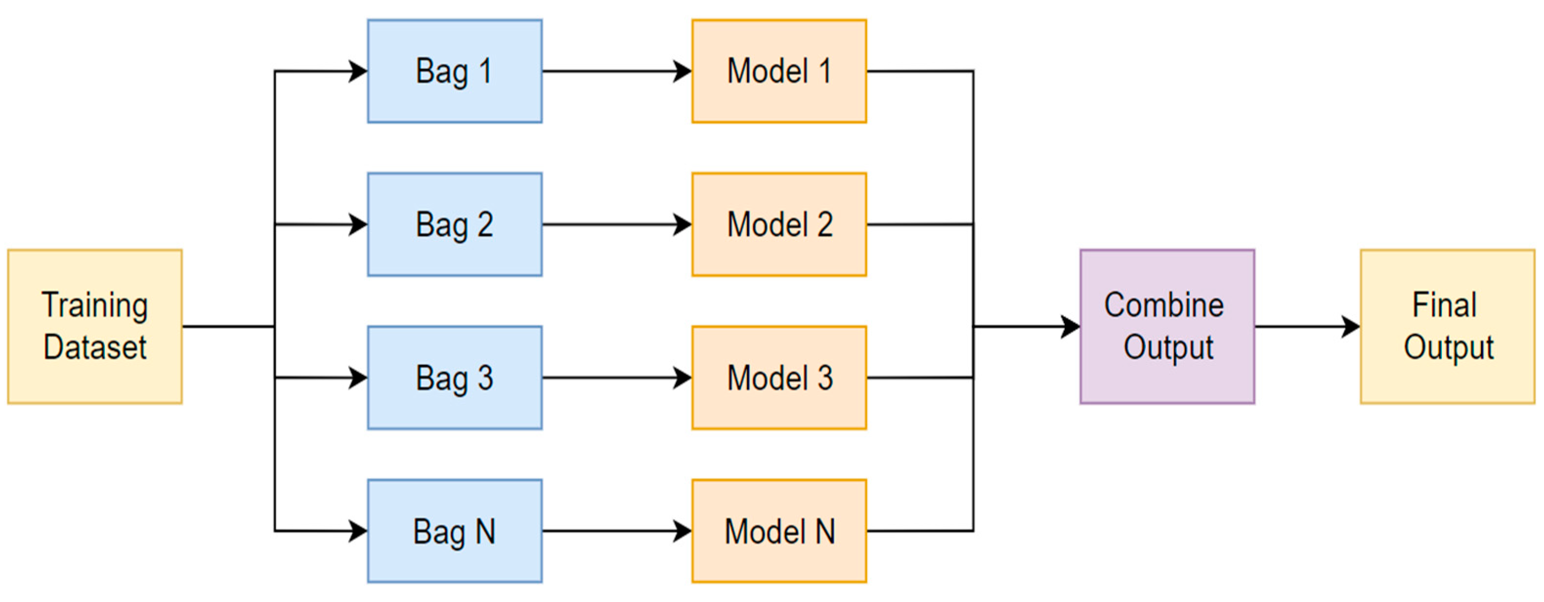
Ensemble learning refers to the use of multiple machine learning models working together to improve predictive accuracy, stability, and generalisation performance compared to using a single model [113]. This method helps reduce overfitting and minimises errors by combining the strengths of different algorithms. Boosting, bagging, and stacking are the three primary ensemble techniques, each with unique mechanisms for constructing and combining models [114]. Understanding the differences in how each ensemble method operates is important when selecting the most appropriate approach for specific data challenges, especially in environmental modelling.

5.1. Bagging Method

Bagging, which stands for bootstrap aggregating, involves generating multiple datasets through resampling from the original dataset and training base learners on these samples [115]. The goal is to reduce variance by averaging the outputs of models trained on different versions of the data. Figure 3 illustrates the bagging process, where samples are passed into several base models and their results are combined either by majority vote for classification or by averaging for regression tasks [116]. Bagging is particularly effective for high-variance models like decision trees, which are sensitive to data fluctuations. By averaging their predictions, bagging creates a more stable and consistent ensemble output.

5.2. Boosting Method

Boosting is a sequential ensemble approach that builds models one after another, with each new model focusing on correcting the mistakes made by the previous one [117]. This process continues until the overall error is minimised, often leading to improved accuracy. In contrast to bagging, boosting gives more weight to misclassified examples, which directs the model to learn difficult patterns. The new model naturally emphasises the findings that have been the hardest to align up until now. This makes the learner better and less biased by the end of the process [118]. Figure 4 shows the boosting framework, where new learners are trained on adjusted data that include previously misclassified examples [119]. Well-known algorithms such as AdaBoost and Gradient Boosting are widely used in many fields [120]. This focus on correcting errors makes boosting suitable for structured data and time-series prediction, although it requires careful parameter tuning to avoid overfitting.

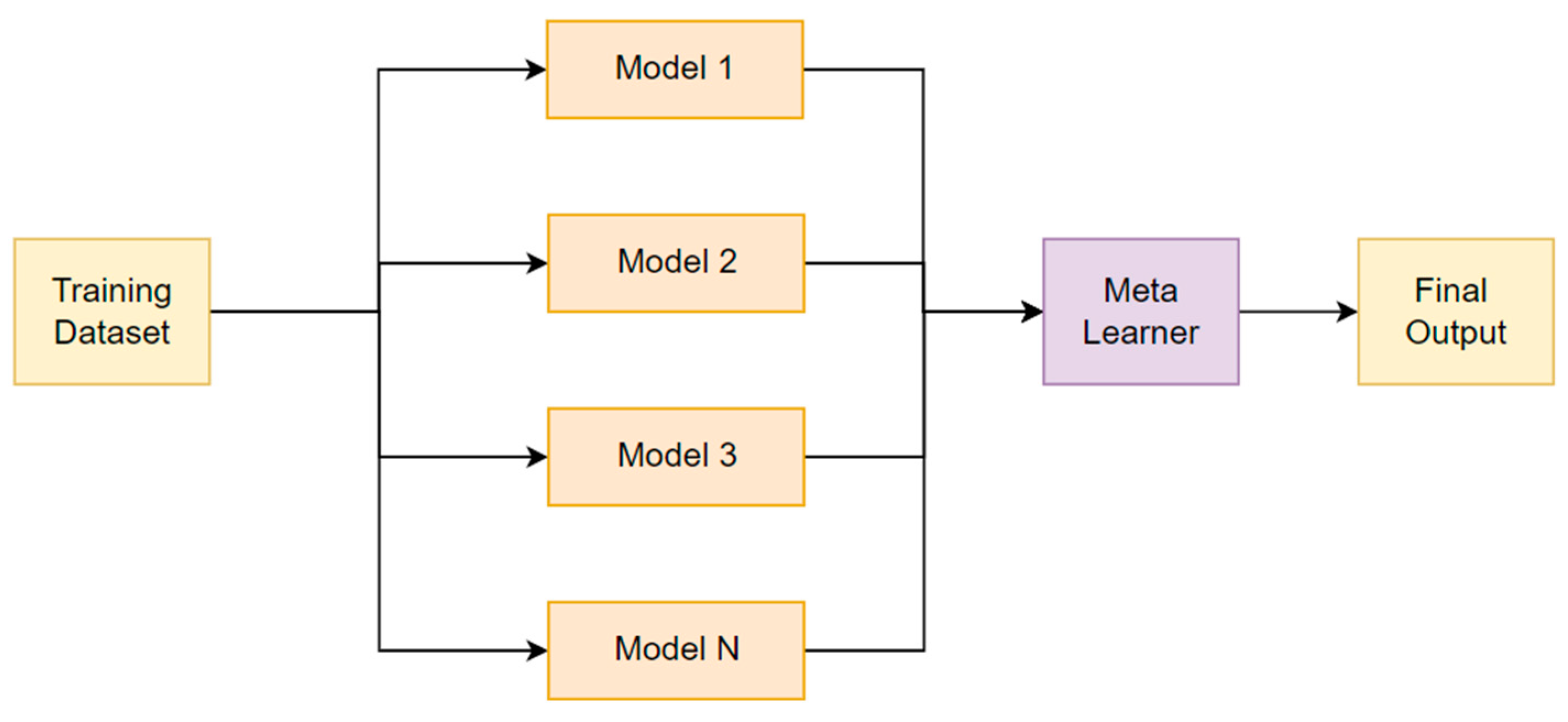
5.3. Stacking Method

Stacking refers to an assembly method where one or more base-level classifiers are combined with a meta-learner classifier. The stacking ensemble model is used to classify skin diseases [121]. The stacking model outperforms traditional classifiers, improving diagnostic accuracy. Stacking is used to estimate crop yield by integrating various machine learning models [122]. A combination of decision trees, random forest, and Gradient Boosting yielded the best prediction results for agricultural productivity. A stacking ensemble is used to predict heart disease risk from multiple datasets [123]. Stacking outperformed individual classifiers in medical diagnostics. The metaclassifier is used to estimate both the input and output of each model, along with the weights [113]. The models that perform the best are selected, while the others are not accepted. Stacking uses a metaclassifier to combine several base classifiers that have been trained with various learning methods on one dataset. Model predictions are combined with inputs from each successive layer to create a new set of predictions [124]. Ensemble stacking refers to mixing since all data is combined to generate a forecast or categorisation. Multi-linear response (MLR) and probability distribution (PD) stacking represent the most advanced techniques available. It is widely recognised that combining multiple base-level classifiers, even with weakly connected predictions, tends to yield effective results. The framework for the stacking approach is illustrated in Figure 5. Various models are applied to the input dataset, and the meta-learner utilises the outputs from all the models to generate the final predictions.

While ensemble methods such as bagging, boosting, and stacking are widely recognised for improving model accuracy, their specific application to water quality modelling, particularly WQI classification, has also been demonstrated. Recent studies have demonstrated the effectiveness of ensemble learning methods, especially in WQI modelling and water quality prediction. For instance, an ISE Europe study deployed random forest (RF) and Gradient Boosting (GB) to forecast the WQI in Malaysia’s Johor River basin, using just three key water parameters. The ensemble models achieved R² values of 0.86 (RF) and 0.85 (GB), achieving correct WQI class prediction in ~96% of cases [125]. Similarly, the authors of [126] applied various tree-based ensembles bagging, RF, Extra Trees, AdaBoost, and XGBoost for data from Vietnam’s An Kim Hai irrigation system. Among them, RF was the top performer for WQI estimation. On a broader scale, a recent study set in Europe devised an optimised ensemble WQI model (combining LR, RF, and XGB) that outperformed traditional methods by exhibiting RMSE = 0.0034, R² ≈ 1.00, and strong robustness to outliers [127]. These studies illustrate the empirical value of ensemble models in water-related contexts and validate their inclusion in environmental ML pipelines.

6. Statistical Analysis of Water Quality

Datasets on water quality often exhibit non-normality, the presence of outliers, missing data, low values that fall below detection thresholds, and serial dependence. To ensure the validity of results and the formulation of practical suggestions in the field of water prediction, it is imperative to employ appropriate statistical methodologies when analysing data pertaining to water quality. There is a wide range of statistical analyses available for the analysis of water quality data. Statistical techniques in machine learning offer a complete framework for evaluating the resilience, efficiency, and dependability of models. These techniques are crucial for assessing the performance of models, identifying possible problems, and guaranteeing correct predictions when the models are used with real-world data.

Graphing, trend analysis, correlation analysis, regression analysis, and time series analysis are among the frequently utilised statistical procedures [128]. Graphs are valuable tools for visually summarising data, as they offer a concise and lucid representation of essential information inherent in the data under analysis [129]. The necessity for more comprehensive models can be evaluated by visual examination utilising methods such as boxplots, scatter plots, and Q-Q plots [130]. In this chapter, five methods are reviewed, which include residual analysis, diagnostic and assumption tests, feature importance, learning curve analysis, and principal component analysis (PCA).

6.1. Residual Analysis

Residual analysis and error analysis are closely related analyses; both measure a distance (deviation or error) [131]. Residual analysis is a crucial component of regression analysis, serving as a diagnostic tool to evaluate the appropriateness of a model’s fit to the observed data [132]. It is crucial to evaluate the validity of the assumptions that underlie the regression analysis when using a regression model to predict outcomes based on predictor variables. The main assumptions consist of linearity, independence, homoscedasticity, and normality of residuals [133]. The method commences by computing the residuals, which represent the discrepancies between the observed values and the values anticipated by the model. Subsequently, these residuals are graphed against the expected values in order to visually examine any discernible trends. An ideal model should have a random distribution of residuals along the horizontal axis, indicating that it accurately captures the underlying pattern without any systematic errors.

6.2. Diagnostic and Assumption Tests

Diagnostic and assumption tests validate the suitability of statistical models by checking assumptions such as normality, multicollinearity, and autocorrelation, using methods like the Shapiro–Wilk test for normality or the Breusch–Pagan test for homoscedasticity [134]. The presence of patterns in this plot, such as curved relationships or a spread that resembles a fan shape, can be indicative of issues such as non-linearity or heteroscedasticity, respectively. Statistical tests enhance and supplement these visual examinations. The Shapiro–Wilk test is frequently employed to evaluate the normality of the residuals [135]. The assumption of normality is crucial in numerous regression models that employ the least-square estimation approach, as it forms the foundation for ensuring the statistical tests for coefficients are accurate.

To assess homoscedasticity, statistical procedures such as the Breusch–Pagan test or White’s test are utilised to verify that the residual variance remains constant across various levels of anticipated values [136]. Having a consistent variance in predictions ensures that the coefficient estimation remains reliable and stable throughout the whole range of data. A different study utilises the Breusch–Pagan test for random effects to determine whether to select the random-effect regression or the ordinary least-square regression [137]. The test results indicate a preference for random-effect generalised least-square regression.

6.3. Feature Importance

Feature importance provides insights into the influence of predictors on the target variable, helping to simplify models and improve interpretability. The evaluation of feature importance serves as a crucial analytical technique used after the initial deployment of a model to determine the input factors that have a substantial impact on the model’s predictions [138]. For classification tasks, this impurity is often measured using Gini impurity, while for regression tasks, it is measured by the reduction in variance. The feature analysis indicates that the number of trademark authorisations significantly influences prediction accuracy, demonstrating the practical application of feature importance for optimising algorithm models in economic forecasting [139]. A different study discusses feature importance analysis, indicating that band values and vegetation indices significantly influence classification results [140]. The Marginal Contribution Feature Importance (MCI) metric quantifies the individual impact of features while addressing complex inter-feature correlations, which is useful in regression contexts [141]. Additionally, another article examines the role of feature importance in explainable AI, utilising contextual importance methods to clarify how features influence both regression and classification outcomes, thereby enhancing model transparency [142]. These studies demonstrate the critical role of feature importance analysis in improving model interpretability and predictive accuracy across various domains.

6.4. Learning Curve Analysis

Learning curve analysis is crucial for assessing the efficiency of a model’s learning process as the quantity of training data grows [143]. It can determine whether augmenting the dataset, escalating the intricacy of the model, or simplifying the model can improve performance. The learning curves are applied to optimise regression algorithms in wireless sensor networks (WSNs), providing insights into high-bias and variance issues in statistical modelling [144]. In healthcare, learning curve analysis is utilised to evaluate emergency physicians’ skill development in point-of-care ultrasound (POCUS), identifying the steep acquisition phase and the levelling-off point as experience increases [145]. Additionally, another study introduces a novel method for ranking normalised entropy curves in automated machine learning systems, showcasing how learning curve analysis optimises model configurations and enhances decision-making [146]. These applications highlight the versatility of learning curve analysis in improving modelling efficiency, understanding skill progression, and optimising computational resources. The relationship between the size of the training set and the error rates can be better understood by looking at the learning curve, which helps to uncover patterns in the data.

6.5. Principal Component Analysis (PCA)

Principal component analysis (PCA) is a technique employed to decrease the number of dimensions in extensive datasets, hence enhancing comprehensibility while minimising the loss of information [147]. It converts the initial variables into a different set of variables, known as principal components, that are linear combinations of the original variables. This strategy is very advantageous for improving the effectiveness and productivity of machine learning models by concentrating on the most important features. The utilisation of data analysis techniques is advantageous in discerning the fundamental framework of the data and determining the factors that have the utmost significance [148].

A recent study introduced the PCA test R package (version 2.1.2) to statistically assess the significance of PCA results, enabling robust applications in ecological and evolutionary datasets [149]. Similarly, PCA’s importance in chemometrics was highlighted for analysing trends in large datasets by reducing complexity in variables and objects [150]. A different study utilised spatio-temporal PCA to address dependencies in multivariate datasets, optimising variance and integrating spatial indices for social sciences [151].

PCA proves essential in integrating with other methodologies. The combination of PCA with Data Envelopment Analysis (DEA) aimed to enhance efficiency measurement indices in state financial management [152]. Additionally, PCA was utilised alongside Fuzzy Subtractive Clustering for enhanced clustering outcomes in high-dimensional datasets [153]. These examples illustrate PCA’s versatility, spanning ecological studies and chemometrics to financial management and machine learning applications, establishing it as an indispensable tool for extracting actionable insights from complex datasets.

Table 6. Previous studies on statistical methods for monitoring water quality.

Ref.	Method	Advantages	Disadvantages	Data Size	Water Parameters
[154]	PCA	In-depth analysis, including national legal compliance and enhancing relevance for management.	Limited to a single lake; results may not generalise to other water bodies.	5-year period (2020–2024).	Temperature, turbidity, pH, conductivity, total alkalinity, total hardness
[54]	Feature Importance (using SHAP)	Uses SHAP for feature contributions, providing insight into key drivers.	Model accuracy declines over longer forecasting horizons (though still R2 > 0.75 up to 30 days).	Dataset size is not stated.	DO, temperature
[155]	Residual Analysis	Achieved high empirical model fits (R2: DO = 0.948, NO3 = 0.858, TP = 0.779).	Based on one-day sampling at 17 sites, limits temporal representativeness.	Dataset size is not stated.	TSS, turbidity, DO, nitrate, TP
[156]	Diagnostic and Assumption Test (Durbin–Watson)	Provides actionable insights with sensitivity analysis (e.g., impacts of rainfall, materials, transport).	Does not evaluate direct water quality parameters.	Dataset size is not stated.	No water-quality analytes
[157]	Learning Curve Analysis	Compares 7 machine learning models, with ensemble Gradient Boosting delivering highest accuracy	Focus on water quality classification, not continuous concentration estimation.	Dataset from 2005 to 2020.	DO, BOD, AN, pH, TSS, COD

summarises recent applications of key statistical analysis techniques in machine learning-based water quality research. It highlights how methods such as PCA are used to reduce complex datasets and identify the most influential water quality parameters. Statistical techniques play a crucial role in enhancing the interpretability and reliability of water quality prediction models. For example, SHAP (SHapley Additive exPlanations) is increasingly used to interpret black-box models by attributing contributions of input features like temperature and pH. However, SHAP can be computationally expensive for complex models and may produce inconsistent explanations when features are highly correlated. Similarly, residual analysis is used to detect systematic errors in regression models, while diagnostic tests such as the Durbin–Watson test help verify assumptions like autocorrelation in time series datasets. Principal component analysis (PCA) is commonly applied to reduce feature dimensionality and highlight key influencing parameters, such as DO or NH₃-N. Additionally, learning curve analysis is useful for assessing model convergence and preventing overfitting during training.

7. Challenges in Machine Learning-Based WQI Modelling and Limitations in Current Studies

7.1. Interpretability, Data Availability, and Complexity of Machine Learning Models

Despite the growing adoption of machine learning (ML) techniques in water quality prediction, several challenges hinder their widespread implementation. One major obstacle is the availability and quality of data. In Malaysia, water quality datasets are often incomplete, inconsistent, or limited to specific locations, especially in rural and under-monitored areas. This presents difficulties for training and validating ML models that require large and well-structured datasets. Moreover, environmental data are subject to seasonal variability, sensor drift, and irregular sampling intervals, which introduce additional noise and uncertainty into modelling efforts.

Another significant challenge is model interpretability. While models such as artificial neural networks (ANNs) and random forests (RF) have demonstrated high predictive accuracy, their internal mechanisms are often opaque, making it difficult for stakeholders to understand how predictions are derived. This “black-box” nature restricts the acceptance of such models by decision-makers who require justifiable outputs. Furthermore, hybrid and deep learning models are computationally intensive, requiring advanced expertise and high-performance computing resources, which may not be accessible to all water management agencies.

Overfitting is another issue, especially in models trained on site-specific data. Such models may perform well within a particular region but fail to generalise to different rivers or catchments due to variations in environmental conditions. Lastly, the lack of standardised frameworks for model evaluation—such as common metrics, validation procedures, and benchmark datasets—makes it difficult to compare results across studies and establish best practices for the Malaysian context.

A review of the existing literature reveals several limitations in ML applications in water quality prediction. First, there is limited integration of Internet of Things (IoT) technologies with predictive models. Although real-time sensor networks are emerging, few studies incorporate live data streams for continuous prediction and anomaly detection. This represents a missed opportunity for proactive water quality management. Another gap lies in the narrow focus on physicochemical parameters alone. Most ML models rely solely on variables such as pH, DO, BOD, COD, and TSS, without considering other relevant data sources like meteorological conditions, land use, or socio-economic activities. Incorporating these additional factors could significantly enhance model accuracy and practical relevance.

Spatial and temporal modelling is also underdeveloped. Many models treat water quality data as static or purely time-based, ignoring the geographical dynamics that influence river systems. The absence of spatio-temporal modelling limits the ability to simulate pollution patterns across river basins. Moreover, explainable AI (XAI) techniques such as SHAP values or decision rule extraction are rarely applied in the Malaysian context, even though they offer clear benefits in improving stakeholder trust and model transparency. Lastly, fuzzy logic-based systems are underutilised in decision-making platforms. While fuzzy logic is well suited to handle uncertainty and vagueness in environmental data, it is seldom integrated into real-time water quality monitoring systems or dashboards. This represents a valuable opportunity for further development in intelligent environmental management tools.

7.2. Cost–Benefit Considerations in Resource-Limited Settings

While complex models such as ANNs, hybrid systems, or ensemble techniques provide superior accuracy, their practical deployment in resource-limited regions raises important feasibility questions. These models often require significant computational resources, regular maintenance, and skilled personnel to operate, factors that may not be present in rural or low-income areas.

Simpler models, such as decision trees or Ridge Regression, may offer lower predictive accuracy but are more accessible for routine monitoring and deployment using low-cost hardware. For instance, microcontrollers such as Raspberry Pi (Cambridge, UK) or Arduino (Monza, Italy) can effectively run lightweight models for on-site water quality assessment with minimal infrastructure. Therefore, model selection should consider not only performance metrics but also long-term sustainability, cost-efficiency, and maintenance requirements.

A balanced approach could involve deploying simpler models for rapid field assessment while reserving complex models for centralised, high-stakes analysis or integration with government-level dashboards. This tiered strategy can help bridge the gap between technical capability and real-world implementation, especially in the context of environmental applications where resources are unevenly distributed.

7.3. Practical Concerns: Data Privacy, Sensor Calibration, and Infrastructure Gaps

Although machine learning offers great potential in water quality prediction, real-world deployment needs to account for several operational risks. First, data privacy becomes a concern in centralised monitoring systems where geotagged or time-sensitive water quality data are continuously streamed. Ensuring compliance with local data governance policies and protecting sensitive ecosystem or industrial information is critical, especially if third-party cloud services are involved.

Second, the accuracy and consistency of raw sensor data are heavily influenced by proper sensor calibration. Inaccurate readings due to uncalibrated or degraded sensors can mislead ML models, causing incorrect predictions or false alerts. This is especially problematic in long-term deployments where manual recalibration is resource-intensive. Automated calibration, quality control routines, or redundancy in sensor systems should be considered during system design.

Finally, infrastructure limitations such as unstable power supply, weak internet connectivity in remote regions, and hardware maintenance pose major constraints for deploying ML-powered systems. Even the most accurate models will fail if the sensors feeding them are unreliable or disconnected. Designing systems with offline capability, edge processing, and minimal maintenance requirements becomes essential, especially for rural or underfunded regions. Addressing these real-world constraints is vital for translating ML research into sustainable environmental monitoring solutions.

8. Conclusions

This review comprehensively examines the integration of machine learning (ML) and statistical methodologies for forecasting and classifying water quality, with particular focus on the Malaysian context. It demonstrates how advancements in ML, including classification, regression, and hybrid models, have significantly enhanced the ability to monitor, assess, and predict water quality parameters. Models such as random forest, support vector machines, ANNs, ARIMA, and ensemble approaches have shown promising accuracy in handling complex, non-linear environmental datasets.

Statistical techniques like residual analysis, learning curve evaluation, PCA, and feature importance further reinforce model validity and interpretability. These tools ensure that models are not only predictive but also explainable and reliable, addressing the critical need for transparency in decision-support systems, particularly in environmental governance.

However, challenges persist that include data quality issues, model generalizability, computational demands, and a lack of real-time, spatially aware data integration. Notably, the limited deployment of explainable AI (XAI), fuzzy logic, and real-time IoT-enabled predictive platforms constrains practical adoption in water management strategies. The black-box nature of some high-performing models also limits trust among policymakers and practitioners. To bridge these gaps, this review calls for strategic interdisciplinary collaborations among environmental scientists, data engineers, and policymakers. Establishing standardised datasets, benchmarking protocols, and adopting transparent modelling frameworks are vital next steps. Furthermore, integrating ML with smart sensors, remote sensing, and cloud-based systems can enable real-time, adaptive water quality monitoring solutions. Ultimately, this study affirms that while ML techniques hold transformative potential for sustainable water management, their success depends on robust data infrastructure, interdisciplinary cooperation, and the adoption of explainable and inclusive technologies. As Malaysia and other nations face growing water security challenges, the future of water quality management will increasingly rely on the effective fusion of AI-driven analytics with policy and environmental insight.

To overcome the current limitations and build more robust and useful water quality prediction systems, several future directions are proposed. First, national agencies and academic institutions should collaborate to develop open-access benchmark datasets and standardised evaluation protocols. This would ensure consistency, facilitate model comparison, and accelerate research progress in the Malaysian context. Second, interdisciplinary model design should be promoted. Collaborations between hydrologists, environmental scientists, computer engineers, and machine learning experts can lead to more accurate, interpretable, and policy-relevant models. Future research should also explore the integration of explainable AI (XAI) techniques to improve transparency and acceptance, especially in public sector applications. Thus, the next generation of ML-based water quality models should prioritise accuracy, interpretability, adaptability, and qualities that are essential for ensuring sustainable water management.

References

1. Munteanu, C.; Teoibas-Serban, D.; Iordache, L.; Balaurea, M.; Blendea, C.D. Water intake meets the Water from inside the human body—Physiological, cultural, and health perspectives—Synthetic and Systematic literature review. Balneo PRM Res. J. 2021, 12, 196–209. [Google Scholar] [CrossRef]
2. Angelakis, A.N.; Valipour, M.; Choo, K.-H.; Ahmed, A.T.; Baba, A.; Kumar, R.; Toor, G.S.; Wang, Z. Desalination: From Ancient to Present and Future. Water 2021, 13, 2222. [Google Scholar] [CrossRef]
3. World Health Organization. Drinking-Water. Available online: https://www.who.int/news-room/fact-sheets/detail/drinking-water (accessed on 7 June 2024).
4. He, C.; Liu, Z.; Wu, J.; Pan, X.; Fang, Z.; Li, J.; Bryan, B.A. Future global urban water scarcity and potential solutions. Nat. Commun. 2021, 12, 4667. [Google Scholar] [CrossRef]
5. Kumar, S. The Looming Threat of Water Scarcity. Vital Signs 2013, 20, 96–100. [Google Scholar] [CrossRef]
6. TayyabZahid, A.M.; Munir, A.; Falk, M.; Muazim, M.; Umair, M.; Qasim, S.; Khan, D.G. Chronic Effect of Heavy Metal Exposure on Poultry Health and Performance. Biol. Times 2024, 3, 1–2. [Google Scholar]
7. Limburg, K.E. Deoxygenation—Coming to a water body near you. Front. Ecol. Environ. 2024, 22, e2812. [Google Scholar] [CrossRef]
8. Mutono, N.; Wright, J.; Mutembei, H.; Muema, J.; Thomas, M.; Mutunga, M.; Thumbi, S.M. The nexus between improved water supply and water-borne diseases in urban areas in Africa: A scoping review protocol. AAS Open Res. 2020, 3, 1–17. [Google Scholar] [CrossRef] [PubMed]
9. Park, J.; Kim, K.T.; Lee, W.H. Recent Advances in Information and Communications Technology (ICT) and Sensor Technology for Monitoring Water Quality. Water 2020, 12, 510. [Google Scholar] [CrossRef]
10. Ghiță, S.; Stanciu, I.; Sabău, A. Assessment of the Quality of the Aquatic Environment in the Areas Bordering the Development of Fishing Activities. J. Mar. Technol. Environ. 2023, 2, 32–37. [Google Scholar] [CrossRef]
11. Nagothu, S.K.; Sri, P.B.; Anitha, G.; Vincent, S.; Kumar, O.P. Advancing aquaculture: Fuzzy logic-based water quality monitoring and maintenance system for precision aquaculture. Aquac. Int. 2025, 33, 32. [Google Scholar] [CrossRef]
12. Nasution, S.F.; Harmadi, H.; Suryadi, S.; Widiyatmoko, B. Development of River Flow and Water Quality Using IOT-based Smart Buoys Environment Monitoring System. J. ILMU Fis. Univ. Andalas 2023, 16, 1–12. [Google Scholar] [CrossRef]
13. Dewangan, S.K.; Toppo, D.N.; Kujur, A. Investigating the Impact of pH Levels on Water Quality: An Experimental Approach. Int. J. Res. Appl. Sci. Eng. Technol. 2023, 11, 756–759. [Google Scholar] [CrossRef]
14. Dada, M.A.; Majemite, M.T.; Obaigbena, A.; Daraojimba, O.H.; Oliha, J.S.; Nwokediegwu, Z.Q.S. Review of smart water management: IoT and AI in water and wastewater treatment. World J. Adv. Res. Rev. 2024, 21, 1373–1382. [Google Scholar] [CrossRef]
15. Abuzir, S.Y.; Abuzir, Y.S. Machine learning for water quality classification. Water Qual. Res. J. 2022, 57, 152–164. [Google Scholar] [CrossRef]
16. Yan, X.; Zhang, T.; Du, W.; Meng, Q.; Xu, X.; Zhao, X. A Comprehensive Review of Machine Learning for Water Quality Prediction over the Past Five Years. J. Mar. Sci. Eng. 2024, 12, 159. [Google Scholar] [CrossRef]
17. Sahu, P.; Londhe, S.N.; Kulkarni, P.S. Modelling water quality parameters using model tree, random forest, and non-linear regression for Mula-Mutha River, Pune, India. Environ. Monit. Assess. 2024, 196, 1047. [Google Scholar] [CrossRef]
18. Jude, P.S.V.; Brighty, S.P.S.; Gandhi, R.R.; Balamurguan, K.; Krishnakumar, R. Water Quality Prediction Using Random Forest Algorithm. In Proceedings of the 2nd International Conference on Futuristic Technologies (INCOFT), Joondalup, Australia, 24–26 November 2023; Institute of Electrical and Electronics Engineers: Piscataway, NJ, USA, 2023. [Google Scholar] [CrossRef]
19. Li, Z.; Fantke, P. Toward harmonizing global pesticide regulations for surface freshwaters in support of protecting human health. J. Environ. Manag. 2022, 301, 113909. [Google Scholar] [CrossRef] [PubMed]
20. Graham, D.J.; Bierkens, M.F.P.; van Vliet, M.T.H. Impacts of droughts and heatwaves on river water quality worldwide. J. Hydrol. 2024, 629, 130590. [Google Scholar] [CrossRef]
21. Mitchell, E.J.; Frisbie, S.H. A comprehensive survey and analysis of international drinking water regulations for inorganic chemicals with comparisons to the World Health Organization’s drinking-water guidelines. PLoS ONE 2023, 18, e0287937. [Google Scholar] [CrossRef] [PubMed]
22. Tyurina, I.A.; Ya, L.-S.; Manaeva, E.S. Legislation of the countries of the European Region on the drinking water quality management (overview). Vodosnabzhenie Sanit. Teh. 2022, 10, 14–22. [Google Scholar] [CrossRef]
23. Hendrayana, H.; Riyanto, I.A.; Nuha, A. River water quality variability in the young volcanic areas in Java, Indonesia. J. Degrad. Min. Lands Manag. 2023, 10, 4467–4478. [Google Scholar] [CrossRef]
24. Van Winckel, T.; Cools, J.; Vlaeminck, S.E.; Joos, P.; Van Meenen, E.; Borregán-Ochando, E.; Steen, K.V.D.; Geerts, R.; Vandermoere, F.; Blust, R. Towards harmonization of water quality management: A comparison of chemical drinking water and surface water quality standards around the globe. J. Environ. Manag. 2021, 298, 113447. [Google Scholar] [CrossRef]
25. Wang, X.; Xu, X.Q.; Gao, C.H.; Li, L.H.; Liu, Y.; Zhang, N.; Xia, Y.; Fang, X.; Zhang, X.G. Assessing the drinking water quality in the Inner Mongolia Autonomous Region from 2014 to 2018. J. Water Health 2022, 20, 610–619. [Google Scholar] [CrossRef]
26. Karmakar, B.; Singh, M.K. Assessment of water quality status of water bodies using water quality index and correlation analysis in and around industrial areas of west District, Tripura, India. Nat. Environ. Pollut. Technol. 2021, 20, 551–559. [Google Scholar] [CrossRef]
27. Enea, A.; Hapciuc, O.-E.; Iosub, M.; Minea, I.; Romanescu, G. Water quality assessment in three mountainous watersheds from Eastern Romania (Suceava, Ozana and Tazlau rivers). Environ. Eng. Manag. J. 2017, 16, 605–614. Available online: https://eemj.eu/index.php/EEMJ/article/view/3211 (accessed on 2 November 2024). [CrossRef]
28. DOE. National Water Quality Standards and Water Quality Index—Department of Environment. Available online: https://www.doe.gov.my/en/national-river-water-quality-standards-and-river-water-quality-index/ (accessed on 12 April 2024).
29. Goi, C.L. The river water quality before and during the Movement Control Order (MCO) in Malaysia. Case Stud. Chem. Environ. Eng. 2020, 2, 100027. [Google Scholar] [CrossRef]
30. Yeoh, R.S.Y.; Wong, K.Y. Water’s role in ensuring food security: An analysis of Malaysia from 1991 to 2020. In Proceedings of the 12th International Conference on Business, Accounting, Finance and Economics (BAFE 2024), Kampar, Malaysia, 23 October 2024. [Google Scholar]
31. Najah, A.; Teo, F.Y.; Chow, M.F.; Huang, Y.F.; Latif, S.D.; Abdullah, S.; Ismail, M.; El-Shafie, A. Surface water quality status and prediction during movement control operation order under COVID-19 pandemic: Case studies in Malaysia. Int. J. Environ. Sci. Technol. 2021, 18, 1009–1018. [Google Scholar] [CrossRef]
32. Alberti, G.; Zanoni, C.; Magnaghi, L.R.; Biesuz, R. Low-cost, disposable colourimetric sensors for metal ions detection. J. Anal. Sci. Technol. 2020, 11, 30. [Google Scholar] [CrossRef]
33. Bernama 29 Polluted Rivers Identified in 2022|MalaysiaNow. 2023. Available online: https://www.malaysianow.com/news/2023/06/13/29-polluted-rivers-identified-in-2022 (accessed on 21 August 2023).
34. Bernama—WST 2040 to Boost Malaysia’s GDP and Water Sector Growth—DPM Fadillah. Bernama. 2024. Available online: https://www.bernama.com/tv/news.php?id=2357799 (accessed on 30 October 2024).
35. Sakke, N.; Jafar, A.; Dollah, R.; Asis, A.H.B.; Mapa, M.T.; Abas, A. Water Quality Index (WQI) Analysis as an Indicator of Ecosystem Health in an Urban River Basin on Borneo Island. Water 2023, 15, 2717. [Google Scholar] [CrossRef]
36. Mamat, N.; Razali, S.F.M.; Hamzah, F.B. Enhancement of water quality index prediction using support vector machine with sensitivity analysis. Front. Environ. Sci. 2023, 10, 1061835. [Google Scholar] [CrossRef]
37. Fadzillah, N.; Salim, A.; Kasmin, H. Study on the Water Quality Index (WQI) of Parit Besar River in Batu Pahat. J. Adv. Environ. Solut. Resour. Recovery 2022, 2, 8–14. [Google Scholar] [CrossRef]
38. Kamarudin, M.K.A.; Wahab, N.A.; Jalil, N.A.A.; Sunardi; Saad, M.H.M. Water quality issues in water resources management at Kenyir Lake, Malaysia. J. Teknol. 2020, 82, 1–11. [Google Scholar] [CrossRef]
39. Encinas, C.; Ruiz, E.; Cortez, J.; Espinoza, A. Design and implementation of a distributed IoT system for the monitoring of water quality in aquaculture. In Proceedings of the 2017 Wireless Telecommunications Symposium, Chicago, IL, USA, 26–28 April 2017; Institute of Electrical and Electronics Engineers: Piscataway, NJ, USA, 2017. [Google Scholar] [CrossRef]
40. De Zuane, J. Handbook of Drinking Water Quality; Wiley: Hoboken, NJ, USA, 1996. [Google Scholar] [CrossRef]
41. Division, E.S. Drinking Water Quality Standard Malaysia; Ministry of Health Malaysia: Putrajaya, Malaysia, 2016. [Google Scholar]
42. Al-Tameemi, H.J.; Jabbar, M. BOD: COD Ratio as Indicator for Wastewater and Industrial Water Pollution. Int. J. Spec. Educ. 2022, 3, 2164–2171. Available online: https://www.researchgate.net/publication/362053527_BOD_COD_Ratio_as_Indicator_for_Wastewater_and_Industrial_Water_Pollution (accessed on 22 April 2024).
43. Liu, Y.Z.; Chen, Z. Prediction of biochemical oxygen demand with genetic algorithm-based support vector regression. Water Qual. Res. J. 2023, 58, 87–98. [Google Scholar] [CrossRef]
44. Mekaoussi, H.; Heddam, S.; Bouslimanni, N.; Kim, S.; Zounemat-Kermani, M. Predicting biochemical oxygen demand in wastewater treatment plant using advance extreme learning machine optimized by Bat algorithm. Heliyon 2023, 9, e21351. [Google Scholar] [CrossRef]
45. Qi, M.; Han, Y.; Zhao, Z.; Li, Y. Integrated determination of chemical oxygen demand and biochemical oxygen demand. Pol. J. Environ. Stud. 2021, 30, 1785–1794. [Google Scholar] [CrossRef]
46. Adjovu, G.E.; Stephen, H.; James, D.; Ahmad, S. Measurement of Total Dissolved Solids and Total Suspended Solids in Water Systems: A Review of the Issues, Conventional, and Remote Sensing Techniques. Remote Sens. 2023, 15, 3534. [Google Scholar] [CrossRef]
47. Wu, J.; Wang, Z. A Hybrid Model for Water Quality Prediction Based on an Artificial Neural Network, Wavelet Transform, and Long Short-Term Memory. Water 2022, 14, 610. [Google Scholar] [CrossRef]
48. Shams, M.Y.; Elshewey, A.M.; El-kenawy, E.S.M.; Ibrahim, A.; Talaat, F.M.; Tarek, Z. Water quality prediction using machine learning models based on grid search method. Multimed. Tools Appl. 2024, 83, 35307–35334. [Google Scholar] [CrossRef]
49. Fang, P.; Wang, Y.; Zhao, Y.; Kang, J. Analysis of Prediction Confidence in Water Quality Forecasting Employing LSTM. Water 2025, 17, 1050. [Google Scholar] [CrossRef]
50. Abushandi, E. Water Quality Assessment and Forecasting Along the Liffey and Andarax Rivers by Artificial Neural Network Techniques Toward Sustainable Water Resources Management. Water 2025, 17, 453. [Google Scholar] [CrossRef]
51. Chen, J.; Wei, X.; Liu, Y.; Zhao, C.; Liu, Z.; Bao, Z. Deep Learning for Water Quality Prediction—A Case Study of the Huangyang Reservoir. Appl. Sci. 2024, 14, 8755. [Google Scholar] [CrossRef]
52. Li, B.; Sun, F.; Lian, Y.; Xu, J.; Zhou, J. A Variational Mode Decomposition—Grey Wolf Optimizer—Gated Recurrent Unit Model for Forecasting Water Quality Parameters. Appl. Sci. 2024, 14, 6111. [Google Scholar] [CrossRef]
53. Sukkuea, A.; Akkajit, P.; Suwannarat, K.; Foithong, P.; Afsarimanesh, N.; Alahi, E.E. AI-Driven Time Series Forecasting of Coastal Water Quality Using Sentinel-2 Imagery: A Case Study in the Gulf of Thailand. Water 2025, 17, 1798. [Google Scholar] [CrossRef]
54. Li, Q.; He, J.; Mu, D.; Liu, H.; Li, S. Dissolved Oxygen Modeling by a Bayesian-Optimized Explainable Artificial Intelligence Approach. Appl. Sci. 2025, 15, 1471. [Google Scholar] [CrossRef]
55. Bin Shahid, S.; Rifat, H.R.; Uddin, A.; Islam, M.; Mahmud, Z.; Sakib, K.H.; Roy, A. Hypertuning-Based Ensemble Machine Learning Approach for Real-Time Water Quality Monitoring and Prediction. Appl. Sci. 2024, 14, 8622. [Google Scholar] [CrossRef]
56. Verma, N.; Bhardwaj, D.; Scholar, M.T. Research Paper on Analysing impact of Various Parameters on Water Quality Index. Int. J. Adv. Res. Comput. Sci. 2017, 8, 2496–2498. [Google Scholar]
57. Malek, N.H.A.; Yaacob, W.F.W.; Nasir, S.A.M.; Shaadan, N. Prediction of Water Quality Classification of the Kelantan River Basin, Malaysia, Using Machine Learning Techniques. Water 2022, 14, 1067. [Google Scholar] [CrossRef]
58. Chinnappan, C.V.; William, A.D.J.; Nidamanuri, S.K.C.; Jayalakshmi, S.; Bogani, R.; Thanapal, P.; Syed, S.; Venkateswarlu, B.; Masood, J.A.I.S. IoT-Enabled Chlorine Level Assessment and Prediction in Water Monitoring System Using Machine Learning. Electronics 2023, 12, 1458. [Google Scholar] [CrossRef]
59. Bentley, C.; Junqueira, T.; Dove, A.; Vriens, B. Mass-Balance Modeling of Metal Loading Rates in the Great Lakes. Environ. Res. 2022, 205, 112557. [Google Scholar] [CrossRef]
60. Haghnazar, H.; Cunningham, J.A.; Kumar, V.; Aghayani, E.; Mehraein, M. COVID-19 and urban rivers: Effects of lockdown period on surface water pollution and quality—A case study of the Zarjoub River, north of Iran. Environ. Sci. Pollut. Res. 2022, 29, 27382–27398. [Google Scholar] [CrossRef]
61. Ma, J.; Ding, Y.; Cheng, J.C.P.; Jiang, F.; Xu, Z. Soft detection of 5-day BOD with sparse matrix in city harbor water using deep learning techniques. Water Res. 2020, 170, 115350. [Google Scholar] [CrossRef]
62. Zounemat-Kermani, M.; Seo, Y.; Kim, S.; Ghorbani, M.A.; Samadianfard, S.; Naghshara, S.; Kim, N.W.; Singh, V.P. Can Decomposition Approaches Always Enhance Soft Computing Models? Predicting the Dissolved Oxygen Concentration in the St. Johns River, Florida. Appl. Sci. 2019, 9, 2534. [Google Scholar] [CrossRef]
63. Pu, F.; Ding, C.; Chao, Z.; Yu, Y.; Xu, X. Water-Quality Classification of Inland Lakes Using Landsat8 Images by Convolutional Neural Networks. Remote Sens. 2019, 11, 1674. [Google Scholar] [CrossRef]
64. Kumar, V.; Sharma, A.; Kumar, R.; Bhardwaj, R.; Thukral, A.K.; Rodrigo-Comino, J. Assessment of heavy-metal pollution in three different Indian water bodies by combination of multivariate analysis and water pollution indices. Hum. Ecol. Risk Assess. 2018, 26, 1–16. [Google Scholar] [CrossRef]
65. Chen, L.; Wu, T.; Wang, Z.; Lin, X.; Cai, Y. A novel hybrid BPNN model based on adaptive evolutionary Artificial Bee Colony Algorithm for water quality index prediction. Ecol. Indic. 2023, 146, 109882. [Google Scholar] [CrossRef]
66. Fang, Z.; Wang, Y.; Peng, L.; Hong, H. Predicting flood susceptibility using LSTM neural networks. J. Hydrol. 2021, 594, 125734. [Google Scholar] [CrossRef]
67. Im, Y.; Song, G.; Lee, J.; Cho, M. Deep Learning Methods for Predicting Tap-Water Quality Time Series in South Korea. Water 2022, 14, 3766. [Google Scholar] [CrossRef]
68. Trach, R.; Trach, Y.; Kiersnowska, A.; Markiewicz, A.; Lendo-Siwicka, M.; Rusakov, K. A Study of Assessment and Prediction of Water Quality Index Using Fuzzy Logic and ANN Models. Sustainability 2022, 14, 5656. [Google Scholar] [CrossRef]
69. Zhou, M.; Zhang, Y.; Wang, J.; Shi, Y.; Puig, V. Water Quality Indicator Interval Prediction in Wastewater Treatment Process Based on the Improved BES-LSSVM Algorithm. Sensors 2022, 22, 422. [Google Scholar] [CrossRef]
70. Ghazwani, M.; Begum, M.Y. Computational intelligence modeling of hyoscine drug solubility and solvent density in supercritical processing: Gradient boosting, extra trees, and random forest models. Sci. Rep. 2023, 13, 1–11. [Google Scholar] [CrossRef]
71. Hoque, J.M.Z.; Nor, N.A.; Alelyani, S.; Mohana, M.; Hosain, M. Improving Water Quality Index Prediction Using Regression Learning Models. Int. J. Environ. Res. Public Health 2022, 19, 13702. [Google Scholar] [CrossRef]
72. Alvarez, V.F.; Salazar, D.G.; Figueroa, C.; Corrales, J.C.; Casanova, J.F. Estimation of Water Turbidity in Drinking Water Treatment Plants Using Machine Learning Based on Water and Meteorological Data. Environ. Sci. Proc. 2023, 25, 89. [Google Scholar] [CrossRef]
73. Hasrod, T.; Nuapia, Y.B.; Tutu, H. Comparison of individual and ensemble machine learning models for prediction of sulphate levels in untreated and treated Acid Mine Drainage. Environ. Monit. Assess. 2024, 196, 1–27. [Google Scholar] [CrossRef]
74. Sudhakara, B.; Priyadarshini, R.; Bhattacharjee, S.; Kamath, S.S.; Pruthviraj, U.; Gangadharan, K.V.; Ghosh, S.K. Spatio-Temporal Analysis and Modeling of Coastal Areas for Water Salinity Prediction. In Proceedings of the 2023 IEEE International Students’ Conference on Electrical, Electronics and Computer Science, SCEECS, Bhopal, India, 18–19 February 2023; Institute of Electrical and Electronics Engineers: Piscataway, NJ, USA, 2023. [Google Scholar] [CrossRef]
75. Nasaruddin, N.; Ahmad, A.; Zakaria, S.F.; Ul-Saufie, A.Z.; Osman, M.S. Predicting Kereh River’s Water Quality: A comparative Study of Machine Learning Models. Environ. Behav. Proc. J. 2023, 8, 213–219. [Google Scholar] [CrossRef]
76. Abirami, K.; Radhakrishna, P.C.; Venkatesan, M.A. Water Quality Analysis and Prediction using Machine Learning. In Proceedings of the 2023 12th IEEE International Conference on Communication Systems and Network Technologies (CSNT), Bhopal, India, 8–9 April 2023; Institute of Electrical and Electronics Engineers: Piscataway, NJ, USA, 2023; pp. 241–245. [Google Scholar] [CrossRef]
77. Abbas, F.; Cai, Z.; Shoaib, M.; Iqbal, J.; Ismail, M.; Ullah, A. Uncertainty Analysis of Predictive Models for Water Quality Index: Comparative Analysis of XGBoost, Random Forest, SVM, KNN, Gradient Boosting, and Decision Tree Algorithms. Artif. Intell. Mach. Learn. 2024; in press. [Google Scholar] [CrossRef]
78. Jena, P.; Rahaman, S.M.; DasMohapatra, P.K.; Barik, D.P.; Patra, D.S. Surface Water Quality Assessment, Prediction & Modelling of River Daya in Odisha. Res. Sq. 2022; in press. [Google Scholar] [CrossRef]
79. Gai, R.; Yang, J. Summary of Water Quality Prediction Models Based on Machine Learning. In Proceedings of the 2021 IEEE 23rd International Conference on High Performance Computing & Communications; 7th International Conference on Data Science & Systems; 19th International Conference on Smart City; 7th International Conference on Dependability in Sensor, Cloud & Big Data Systems & Application (HPCC/DSS/SmartCity/DependSys), Haikou, China, 20–22 December 2021; Institute of Electrical and Electronics Engineers: Piscataway, NJ, USA, 2021; pp. 2338–2343. [Google Scholar] [CrossRef]
80. Zhang, H.; Ren, X.; Chen, S.; Xie, G.; Hu, Y.; Gao, D.; Tian, X.; Xiao, J.; Wang, H. Deep optimization of water quality index and positive matrix factorization models for water quality evaluation and pollution source apportionment using a random forest model. Environ. Pollut. 2024, 347, 123771. [Google Scholar] [CrossRef]
81. Swetha, P.; Rasheed, A.H.K.P.; Harigovindan, V.P. Random Forest Regression based Water Quality Prediction for Smart Aquaculture. In Proceedings of the 4th International Conference on Computing and Communication Systems (I3CS), Shillong, India, 16–18 March 2023; Institute of Electrical and Electronics Engineers: Piscataway, NJ, USA, 2023. [Google Scholar] [CrossRef]
82. Tejaswi, T.; Manoj, C.; Naidu, P.V.D.; Santhosh, T.; Akhil, P.V.S.; Ganesan, V. Nexus of Water Quality prediction by ANN. In Proceedings of the 2022 International Conference on Innovative Computing, Intelligent Communication and Smart Electrical Systems (ICSES), Chennai, India, 15–16 July 2022; Institute of Electrical and Electronics Engineers: Piscataway, NJ, USA, 2022. [Google Scholar] [CrossRef]
83. Mohammed, R.; Al-Obaidi, B. Treatability influence of municipal sewage effluent on surface water quality assessment based on Nemerow pollution index using an artificial neural network. IOP Conf. Ser. Earth Environ. Sci. 2021, 877, 012008. [Google Scholar] [CrossRef]
84. Hasnan, M.I.; Jaffar, A.; Thamrin, N.M.; Misnan, M.F.; Yassin, A.I.M.; Ali, M.S.A.M. NARX-based water quality index model of Air Busuk River using chemical parameter measurements. Indones. J. Electr. Eng. Comput. Sci. 2021, 23, 1663–1673. [Google Scholar] [CrossRef]
85. Wu, J.; Zhang, J.; Tan, W.; Lan, H.; Zhang, S.; Xiao, K.; Wang, L.; Lin, H.; Sun, G.; Guo, P. Application of Time Serial Model in Water Quality Predicting. Comput. Mater. Contin. 2023, 74, 67–82. [Google Scholar] [CrossRef]
86. Lokman, A.; Ramasamy, R.K.; Ting, C.Y. Scheduling and Predictive Maintenance for Smart Toilet. IEEE Access 2023, 11, 17983–17999. [Google Scholar] [CrossRef]
87. Zafra-Mejía, C.A.; Rondón-Quintana, H.A.; Urazán-Bonells, C.F. ARIMA and TFARIMA Analysis of the Main Water Quality Parameters in the Initial Components of a Megacity’s Drinking Water Supply System. Hydrology 2024, 11, 10. [Google Scholar] [CrossRef]
88. Ibrahim, H.; Yaseen, Z.M.; Scholz, M.; Ali, M.; Gad, M.; Elsayed, S.; Khadr, M.; Hussein, H.; Ibrahim, H.H.; Eid, M.H.; et al. Evaluation and Prediction of Groundwater Quality for Irrigation Using an Integrated Water Quality Indices, Machine Learning Models and GIS Approaches: A Representative Case Study. Water 2023, 15, 694. [Google Scholar] [CrossRef]
89. Shah, S.M.H.; Yaseen, M.A.; Abba, S.I.; Lawal, D.U.; Aliyu, F.; Al-Qadami, W.H.H.; Mustaffa, Z.; Pande, C.B.; Sammen, S.S.; Aliundi, I.H. Treated Wastewater Assessment to Optimize Agricultural Water Reuse in Al-Qatif Region Saudi Arabia Using Hybrid Machine Learning Techniques. Water Sci. Technol. 2024; in press. [Google Scholar] [CrossRef]
90. Khan, M.S.I.; Islam, N.; Uddin, J.; Islam, S.; Nasir, M.K. Water quality prediction and classification based on principal component regression and gradient boosting classifier approach. J. King Saud Univ. Comput. Inf. Sci. 2022, 34, 4773–4781. [Google Scholar] [CrossRef]
91. Adizue, U.L.; Tura, A.D.; Isaya, E.O.; Farkas, B.Z.; Takács, M. Surface quality prediction by machine learning methods and process parameter optimization in ultra-precision machining of AISI D2 using CBN tool. Int. J. Adv. Manuf. Technol. 2023, 129, 1375–1394. [Google Scholar] [CrossRef]
92. Nair, J.P.; Vijaya, M.S. River Water Quality Prediction and index classification using Machine Learning. J. Phys. Conf. Ser. 2022, 2325, 012011. [Google Scholar] [CrossRef]
93. Zhou, S.; Song, C.; Zhang, J.; Chang, W.; Hou, W.; Yang, L. A Hybrid Prediction Framework for Water Quality with Integrated W-ARIMA-GRU and LightGBM Methods. Water 2022, 14, 1322. [Google Scholar] [CrossRef]
94. Sarma, A.; Shiney, O.J. An Analysis on the Techniques for Water Quality Prediction from Remotely Sensed data. In Proceedings of the IEEE International Conference on Recent Trends in Electronics and Communication: Upcoming Technologies for Smart Systems (ICRTEC 2023), Mysore, India, 10–11 February 2023; Institute of Electrical and Electronics Engineers: Piscataway, NJ, USA, 2023. [Google Scholar] [CrossRef]
95. Shamsuddin, I.I.S.; Othman, Z.; Sani, N.S. Water Quality Index Classification Based on Machine Learning: A Case from the Langat River Basin Model. Water 2022, 14, 2939. [Google Scholar] [CrossRef]
96. Lilhore, U.K.; Singh, R.I. Water Quality Prediction Using Hybrid Classification Model. In Proceedings of the International Conference on Electrical, Computer, Communications and Mechatronics Engineering (ICECCME), Tenerife, Spain, 19–21 July 2023; Institute of Electrical and Electronics Engineers: Piscataway, NJ, USA, 2023. [Google Scholar] [CrossRef]
97. AlZubi, A.A. IoT-based automated water pollution treatment using machine learning classifiers. Environ. Technol. 2024, 45, 2299–2307. [Google Scholar] [CrossRef]
98. Maulani, J.; Sari, M. Komparasi Metode K-Nearest Neighbor (Knn) Dengan Support Vector Machine (Svm) Terhadap Tingkat Akurasi Klasifikasi Kualitas Air. Smart Comp Jurnalnya Orang Pint. Komput. 2023, 12, 430–435. [Google Scholar] [CrossRef]
99. Yang, Q.; Li, Y.; Gao, J. An effective model based on machine learning for water quality prediction after desalination. In Proceedings of the International Conference on Electronic Information Engineering and Data Processing (EIEDP 2023), Nanchang, China, 17–19 March 2023; Volume 12700, pp. 810–814. [Google Scholar] [CrossRef]
100. Pardeshi, S.; Gandre, P.; Poojari, N.; Pansare, S.; Alte, B. Water Quality Analysis from Satellite Images. In Proceedings of the 2023 International Conference on Data Science and Network Security (ICDSNS), Tiptur, India, 28–29 July 2023; Institute of Electrical and Electronics Engineers: Piscataway, NJ, USA, 2023. [Google Scholar] [CrossRef]
101. Abumohsen, M.; Owda, A.Y.; Owda, M.; Abumihsan, A. Hybrid machine learning model combining of CNN-LSTM-RF for time series forecasting of Solar Power Generation. E-Prime Adv. Electr. Eng. Electron. Energy 2024, 9, 100636. [Google Scholar] [CrossRef]
102. Ahmed, R.; Sreeram, V.; Mishra, Y.; Arif, M.D. A review and evaluation of the state-of-the-art in PV solar power forecasting: Techniques and optimization. Renew. Sustain. Energy Rev. 2020, 124, 109792. [Google Scholar] [CrossRef]
103. Le, T. Enhancing Predictive Capabilities of Arima Models by Hybridization—A Case Study on Omxh25 Index. Master’s Thesis, LUT University, Lappeenranta, Finland, 2024. [Google Scholar]
104. Harini, R.S.S.; Amudha, V.; Lakshmi, S.V. Deep Ensemble-based Water Quality Index Prediction and Classification using Randomized Low-Rank Approximation. In Proceedings of the 2023 2nd International Conference on Augmented Intelligence and Sustainable Systems (ICAISS), Trichy, India, 23–25 August 2023; Institute of Electrical and Electronics Engineers: Piscataway, NJ, USA, 2023; pp. 434–439. [Google Scholar] [CrossRef]
105. Enriquez, L.; Saldarriaga, J.; Berardi, L.; Laucelli, D.; Giustolisi, O. Using artificial intelligence models to support water quality prediction in water distribution networks. IOP Conf. Ser. Earth Environ. Sci. 2023, 1136, 012009. [Google Scholar] [CrossRef]
106. Li, Y.; Li, X.; Xu, C.; Tang, X. Dissolved Oxygen Prediction Model for the Yangtze River Estuary Basin Using IPSO-LSSVM. Water 2023, 15, 2206. [Google Scholar] [CrossRef]
107. Jo, J.; Kwak, C.; Kim, J.; Kim, S. Deriving Optimal Analysis Method for Road Surface Runoff with Change in Basin Geometry and Grate Inlet Installation. Water 2022, 14, 3132. [Google Scholar] [CrossRef]
108. Onga, L.; Kattel-Salusoo, E.; Trapido, M.; Preis, S. Oxidation of Aqueous Dexamethasone Solution by Gas-Phase Pulsed Corona Discharge. Water 2022, 14, 467. [Google Scholar] [CrossRef]
109. Saba, E.; Kalwar, I.H.; Unar, M.A.; Memon, A.L.; Pirzada, N. Fuzzy Logic-Based Identification of Railway Wheelset Conicity Using Multiple Model Approach. Sustainability 2021, 13, 10249. [Google Scholar] [CrossRef]
110. Zeng, Y.; Xu, W.; Wang, H.; Zhao, D.; Ding, H. Nitrogen and Phosphorus Removal Efficiency and Denitrification Kinetics of Different Substrates in Constructed Wetland. Water 2022, 14, 1757. [Google Scholar] [CrossRef]
111. Basack, S.; Goswami, G.; Dai, Z.H.; Baruah, P. Failure-Mechanism and Design Techniques of Offshore Wind Turbine Pile Foundation: Review and Research Directions. Sustainability 2022, 14, 12666. [Google Scholar] [CrossRef]
112. Sanchez, R.; Rodriguez, L. Transboundary Aquifers between Baja California, Sonora and Chihuahua, Mexico, and California, Arizona and New Mexico, United States: Identification and Categorization. Water 2021, 13, 2878. [Google Scholar] [CrossRef]
113. Latha, C.B.C.; Jeeva, S.C. Improving the accuracy of prediction of heart disease risk based on ensemble classification techniques. Inform. Med. Unlocked 2019, 16, 100203. [Google Scholar] [CrossRef]
114. Tanuku, S.R.; Kumar, A.A.; Somaraju, S.R.; Dattuluri, R.; Reddy, M.V.K.; Jain, S. Liver Disease Prediction Using Ensemble Technique. In Proceedings of the 8th International Conference on Advanced Computing and Communication Systems (ICACCS), Coimbatore, India, 25–26 March 2022; Institute of Electrical and Electronics Engineers: Piscataway, NJ, USA, 2022; pp. 1522–1525. [Google Scholar] [CrossRef]
115. Ganaie, M.A.; Hu, M.; Malik, A.K.; Tanveer, M.; Suganthan, P.N. Ensemble deep learning: A review. Eng. Appl. Artif. Intell. 2021, 115, 105151. [Google Scholar] [CrossRef]
116. Mahajan, P.; Uddin, S.; Hajati, F.; Moni, M.A. Ensemble Learning for Disease Prediction: A Review. Healthcare 2023, 11, 1808. [Google Scholar] [CrossRef] [PubMed]
117. Sarmah, U.; Borah, P.; Bhattacharyya, D.K. Ensemble Learning Methods: An Empirical Study. SN Comput. Sci. 2024, 5, 924. [Google Scholar] [CrossRef]
118. Ramesh, D.; Katheria, Y.S. Ensemble method based predictive model for analyzing disease datasets: A predictive analysis approach. Health Technol 2019, 9, 533–545. [Google Scholar] [CrossRef]
119. Mienye, I.D.; Sun, Y. A Survey of Ensemble Learning: Concepts, Algorithms, Applications, and Prospects. IEEE Access 2022, 10, 99129–99149. [Google Scholar] [CrossRef]
120. Verma, A.K.; Pal, S.; Kumar, S. Comparison of skin disease prediction by feature selection using ensemble data mining techniques. Inform. Med. Unlocked 2019, 16, 100202. [Google Scholar] [CrossRef]
121. Jaiyeoba, O.; Ogbuju, E.; Yomi, O.T.; Oladipo, F. Development of a Model to Classify Skin Diseases using Stacking Ensemble Machine Learning Techniques. J. Comput. Theor. Appl. 2024, 2, 22–38. [Google Scholar] [CrossRef]
122. Umamaheswari, K.; Madhumathi, R. Predicting Crop Yield Based on Stacking Ensemble Model in Machine Learning. In Proceedings of the 8th International Conference on I-SMAC (IoT in Social, Mobile, Analytics and Cloud) (I-SMAC 2024), Kirtipur, Nepal, 3–5 October 2024; Institute of Electrical and Electronics Engineers: Piscataway, NJ, USA, 2024; pp. 1831–1836. [Google Scholar] [CrossRef]
123. Wu, Y.; Xia, Z.; Feng, Z.; Huang, M.; Liu, H.; Zhang, Y. Forecasting Heart Disease Risk with a Stacking-Based Ensemble Machine Learning Method. Electronics 2024, 13, 3996. [Google Scholar] [CrossRef]
124. Singh, N.; Singh, P. A Stacked Generalization Approach for Diagnosis and Prediction of Type 2 Diabetes Mellitus. Adv. Intell. Syst. Comput. 2020, 990, 559–570. [Google Scholar] [CrossRef]
125. Sidek, L.M.; Mohiyaden, H.A.; Marufuzzaman, M.; Noh, N.S.M.; Heddam, S.; Ehteram, M.; Kisi, O.; Sammen, S.S. Developing an ensembled machine learning model for predicting water quality index in Johor River Basin. Environ. Sci. Eur. 2024, 36, 67. [Google Scholar] [CrossRef]
126. Nguyen, H.D.; Phan, T.T.H. Investigating Ensemble Learning Methods for Predicting Water Quality Index. Lect. Notes Data Eng. Commun. Technol. 2023, 188, 3–12. [Google Scholar] [CrossRef]
127. Rahman, A.; Syeed, M.M.M.; Karim, M.R.; Fatema, K.; Khan, R.H.; Uddin, M.F. An optimized ensemble ML-WQI model for reliable water quality prediction by minimizing the eclipsing and ambiguity issues. Appl. Water Sci. 2025, 15, 1–27. [Google Scholar] [CrossRef]
128. Schreiber, S.G.; Schreiber, S.; Tanna, R.N.; Roberts, D.R.; Arciszewski, T.J. Statistical tools for water quality assessment and monitoring in river ecosystems—A scoping review and recommendations for data analysis. Water Qual. Res. J. 2022, 57, 40–57. [Google Scholar] [CrossRef]
129. Statswork. Applications of Statistical Analyses on Water Quality Data and Its Recent Research Trends. Pioneer Statistical Consulting. Available online: https://statswork.com/blog/applications-of-statistical-analyses-on-water-quality-data-and-its-recent-research-trends/ (accessed on 13 November 2023).
130. Fu, L.; Wang, Y.-G. Statistical Tools for Analyzing Water Quality Data. 2012. Available online: www.intechopen.com (accessed on 26 May 2025).
131. Benko, Ľ.; Munkova, D.; Munk, M.; Benkova, L.; Hajek, P. The use of residual analysis to improve the error rate accuracy of machine translation. Sci. Rep. 2024, 14, 9293. [Google Scholar] [CrossRef] [PubMed]
132. Soleimani, F.; Hajializadeh, D. Bridge seismic hazard resilience assessment with ensemble machine learning. Structures 2022, 38, 719–732. [Google Scholar] [CrossRef]
133. Wang, X.; Mazumder, R.K.; Salarieh, B.; Salman, A.M.; Shafieezadeh, A.; Li, Y. Machine Learning for Risk and Resilience Assessment in Structural Engineering: Progress and Future Trends. J. Struct. Eng. 2022, 148, 03122003. [Google Scholar] [CrossRef]
134. Ohaegbulem, E.U.; Iheaka, V.C. On Remedying the Presence of Heteroscedasticity in a Multiple Linear Regression Modelling. Afr. J. Math. Stat. Stud. 2024, 7, 225–261. [Google Scholar] [CrossRef]
135. Yulia, Y.; Helvira, R.; Tunisa, J. Impact Analysis of Inflation, ROA, FDR, and Financing on Non-Performing Financing in Indonesian Islamic Banks. Dinar J. Ekon. Dan Keuang. Islam 2024, 11, 222–235. [Google Scholar] [CrossRef]
136. Saariniemi, J. Case-study: Twitter Data Analysis by Linear Regression Modelling. 2023. Available online: https://lutpub.lut.fi/handle/10024/166121 (accessed on 17 October 2024).
137. Wang, W.; Melnyk, L.; Kubatko, O.; Kovalov, B.; Hens, L. Economic and Technological Efficiency of Renewable Energy Technologies Implementation. Sustainability 2023, 15, 8802. [Google Scholar] [CrossRef]
138. Zheng, Z.; Yang, Y.; Zhou, J.; Gu, F. Research on Time Series Data Prediction Based on Machine Learning Algorithms. In Proceedings of the 2024 IEEE 2nd International Conference on Control, Electronics and Computer Technology, ICCECT 2024, Jilin, China, 26–28 April 2024; pp. 680–686. [Google Scholar] [CrossRef]
139. Qu, X.; Zhao, F.; Gao, L.; Zhang, Z. The application of machine learning regression algorithms and feature engineering in practical application. In Proceedings of the 2022 10th International Conference on Information Systems and Computing Technology, ISCTech 2022, Guilin, China, 28–30 December 2022; pp. 259–263. [Google Scholar] [CrossRef]
140. Zheng, Z.; Yuan, J.; Yao, W.; Kwan, P.; Yao, H.; Liu, Q.; Guo, L. Fusion of UAV-Acquired Visible Images and Multispectral Data by Applying Machine-Learning Methods in Crop Classification. Agronomy 2024, 14, 2670. [Google Scholar] [CrossRef]
141. Catav, A.; Fu, B.; Zoabi, Y.; Meilik, A.L.W.; Shomron, N.; Ernst, J.; Sankararaman, S.; Gilad-Bachrach, R. Marginal Contribution Feature Importance—An Axiomatic Approach for Explaining Data. In Proceedings of the 38th International Conference on Machine Learning, Online, 18–24 July 2021; Volume 139, p. 1324. Available online: https://pmc.ncbi.nlm.nih.gov/articles/PMC8460841/ (accessed on 17 November 2024).
142. Framling, K. Feature Importance versus Feature Influence and What It Signifies for Explainable AI. Commun. Comput. Inf. Sci. 2023, 1901, 241–259. [Google Scholar] [CrossRef]
143. Oukhouya, H.; El Himdi, K. A comparative study of ARIMA, SVMs, and LSTM models in forecasting the Moroccan stock market. Int. J. Simul. Process Model. 2023, 20, 125–143. [Google Scholar] [CrossRef]
144. Verma, V.K.; Kumar, V. Optimization of Regression algorithms using Learning curve in WSN. In Proceedings of the 2021 International Conference on Advance Computing and Innovative Technologies in Engineering, ICACITE 2021, Greater Noida, India, 4–5 March 2021; pp. 379–382. [Google Scholar] [CrossRef]
145. Hannula, O.; Hällberg, V.; Meuronen, A.; Suominen, O.; Rautiainen, S.; Palomäki, A.; Hyppölä, H.; Vanninen, R.; Mattila, K. Self-reported skills and self-confidence in point-of-care ultrasound: A cross-sectional nationwide survey amongst Finnish emergency physicians. BMC Emerg. Med. 2023, 23, 23. [Google Scholar] [CrossRef]
146. Liu, H.; Yang, S.; Qi, F.; Wang, S. Learning to Rank Normalized Entropy Curves with Differentiable Window Transformation. 2023. Available online: https://arxiv.org/abs/2301.10443v1 (accessed on 17 November 2024).
147. Lu, J.; Gu, J.; Han, J.; Xu, J.; Liu, Y.; Jiang, G.; Zhang, Y. Evaluation of Spatiotemporal Patterns and Water Quality Conditions Using Multivariate Statistical Analysis in the Yangtze River, China. Water 2023, 15, 3242. [Google Scholar] [CrossRef]
148. Ma, X.; Wang, L.; Yang, H.; Li, N.; Gong, C. Spatiotemporal Analysis of Water Quality Using Multivariate Statistical Techniques and the Water Quality Identification Index for the Qinhuai River Basin, East China. Water 2020, 12, 2764. [Google Scholar] [CrossRef]
149. Camargo, A. PCAtest: Testing the statistical significance of Principal Component Analysis in R. PeerJ 2022, 10, e12967. [Google Scholar] [CrossRef]
150. Brereton, R.G. Principal components analysis with several objects and variables. J. Chemom. 2023, 37, e3408. [Google Scholar] [CrossRef]
151. Krzyśko, M.; Nijkamp, P.; Ratajczak, W.; Wołyński, W.; Wenerska, B. Spatio-temporal principal component analysis. Spat Econ. Anal. 2024, 19, 8–29. [Google Scholar] [CrossRef]
152. Mohammed, A.H.; Ashour, M.A.H. Improving the efficiency measurement index using principal component analysis (PCA). Int. J. Health Sci. 2022, 6, 6584–6600. [Google Scholar] [CrossRef]
153. Haryati, A.E.; Sugiyarto. Clustering with Principal Component Analysis and Fuzzy Subtractive Clustering Using Membership Function Exponential and Hamming Distance. In Proceedings of the 5th International Conference on Information Technology and Digital Applications (ICITDA 2020), Yogyakarta, Indonesia, 13–14 November 2020; IOP Conference Series: Materials Science and Engineering. IOP Publishing Ltd.: Bristol, UK, 2021; Volume 012019, p. 1077. [Google Scholar] [CrossRef]
154. Abalasei, M.E.; Toma, D.; Teodosiu, C. Monitoring and Evaluation of Water Quality from Chirita Lake, Romania. Water 2025, 17, 1844. [Google Scholar] [CrossRef]
155. Padilla-Mendoza, C.; Torres-Bejarano, F.; Campo-Daza, G.; González-Márquez, L.C. Potential of Sentinel Images to Evaluate Physicochemical Parameters Concentrations in Water Bodies—Application in a Wetlands System in Northern Colombia. Water 2023, 15, 789. [Google Scholar] [CrossRef]
156. Zhao, Z.; Liu, C.; Xie, H.; Li, Y.; Zhu, C.; Liu, M. Carbon Accounting and Carbon Emission Reduction Potential Analysis of Sponge Cities Based on Life Cycle Assessment. Water 2023, 15, 3565. [Google Scholar] [CrossRef]
157. Korchagin, S.; Grigoriev, S.; Nguyen, H.V.; Byeon, H. Prediction of Parkinson’s Disease Depression Using LIME-Based Stacking Ensemble Model. Mathematics 2023, 11, 708. [Google Scholar] [CrossRef]
Figure 1. The machine learning models for regression, classification, and hybrid models.
Water 17 02243 g001
Figure 2. The ANFIS model structure for wastewater.
Water 17 02243 g002
Figure 3. Steps taken in the bagging methods.
Water 17 02243 g003
Figure 4. The framework used in the boosting method.
Water 17 02243 g004
Figure 5. The framework used in the stacking methods.
Water 17 02243 g005