The Impact of Hydrogeological Properties on Mass Displacement in Aquifers: Insights from Implementing a Mass-Abatement Scalable System Using Managed Aquifer Recharge (MAR-MASS)

Abstract

This study examines the use of a mass-abatement scalable system with managed aquifer recharge (MAR-MASS) as a sustainable solution for restoring salinized aquifers and improving water quality by removing dissolved salts. It offers a practical remediation approach for aquifers affected by salinization in coastal regions, agricultural areas, and contaminated sites, where variable-density flow poses a challenge. Numerical simulations assessed hydrogeological properties such as hydraulic conductivity, anisotropy, specific yield, mechanical dispersion, and molecular diffusion. A conceptual model integrated hydraulic conditions with spatial and temporal discretization using the FLOPY API for MODFLOW 6 and the IFM API for FEFLOW 10. Python algorithms were run within the high-performance computing (HPC) server, executing simulations in parallel to efficiently process a large number of scenarios, including both preprocessing input data and post-processing results. The study simulated 6950 scenarios, each modeling flow and transport processes over 3000 days of method implementation and focusing on mass extraction efficiency under different initial salinity conditions (3.5 to 35 kg/m³). The results show that the MAR-MASS effectively removed salts from aquifers, with higher hydraulic conductivity prolonging mass removal efficiency. Of the scenarios, 88% achieved potability (0.5 kg/m³) in under five years; among these, 79% achieved potability within two years, and 92% of cases with initial concentrations of 3.5–17.5 kg/m³ reached potability within 480 days. This study advances scientific knowledge by providing a robust model for optimizing managed aquifer recharge, with practical applications in rehabilitating salinized aquifers and improving water quality. Future research may explore MAR-MASS adaptation for diverse hydrogeological contexts and its long-term performance.

1. Introduction

Groundwater management faces critical challenges due to increasing water demand, aquifer salinization, and the effects of climate change [1,2]. Overexploitation, driven by population growth and agricultural expansion, has led to declining water table levels, water quality deterioration, and saline intrusion in coastal aquifers [3,4,5]. Human activities have often exacerbated aquifer salinization, affecting the availability of drinking water, agriculture, and biodiversity.

Managed aquifer recharge (MAR) has emerged as a sustainable strategy for restoring underground reserves and improving water quality through induced filtration [6]. This technique enhances resilience to extreme climatic events and balances water supply and demand [7]. In particular, MAR is an effective solution for mitigating aquifer salinization by enabling the controlled injection of treated water, such as purified wastewater or rainwater, to displace saline water and improve the quality of the resources that are available for human consumption and agriculture [8].

However, implementing MAR techniques presents significant challenges that may limit their effectiveness. One of the main issues is the flow dynamics of water with different densities due to aquifer salinization. This phenomenon leads to the formation of the saline wedge, which naturally develops in coastal aquifers at the interface with the ocean or arises artificially when freshwater injection attempts to displace saline water. Insufficient knowledge about the interaction between saline water and injected freshwater under certain hydrogeological conditions can compromise the efficiency of MAR systems in improving water quality and ensuring a reliable supply [9].

Moreover, adapting these techniques to the specific conditions of each aquifer is crucial. Hydrogeological properties such as hydraulic conductivity, anisotropy, specific yield, mechanical dispersion, and molecular diffusion vary significantly between regions, making it essential to develop customized strategies that optimize the efficiency of MAR systems [10,11].

This research proposes a new approach to managed aquifer recharge, the MAR-MASS method (mass-abatement scalable system using MAR), which is designed to optimize the removal of dissolved salts from groundwater. Through modular configurations, MAR-MASS combines controlled injections and extractions to enhance mass transport dynamics in aquifers affected by salinization.

Compared to traditional MAR strategies, such as positive, negative, or mixed hydraulic barriers, the MAR-MASS introduces significant innovation by enabling vertically distributed injection and extraction. This configuration improves the control of the hydraulic front and enhances the uniform displacement of dense saline masses along the entire aquifer thickness [9,12,13]. While conventional methods often face limitations under variable-density flow conditions, such as inefficient salt mass removal, excessive energy demand, or stagnation in heterogeneous media, the MAR-MASS demonstrates greater operational efficiency compared to standard approaches [14], extending its applicability even to aquifers with low permeability or strong anisotropy [11,15]. The modular and scalable design of the MAR-MASS also addresses key shortcomings of traditional pump-and-treat systems, which frequently underperform in heterogeneous environments [16,17]. By promoting faster remediation, reducing energy requirements, and avoiding pressure overload, the MAR-MASS provides a more sustainable alternative for salinized groundwater recovery.

The primary objective of this study is to assess the effectiveness of the MAR-MASS method in salt removal under different scenarios of hydraulic conductivity, anisotropy, initial salt concentrations, specific yield, mechanical dispersion, and molecular diffusion. A robust conceptual model integrated hydraulic properties, boundary conditions, and appropriate spatial and temporal discretization to achieve this goal. A total of 6950 scenarios were analyzed using numerical models developed in both FEFLOW and MODFLOW, with Python algorithms handling data preprocessing and post-processing. This approach enabled the generation and evaluation of various recharge configurations, the optimization of mass extraction, and the development of practical solutions to mitigate aquifer salinization. The findings of this research reinforce the need for innovative and sustainable approaches in water resource management, promoting practices that enhance water resilience and global sustainable development. Additionally, the finding also lay the groundwork for future hydrogeological research, contributing to the implementation of more efficient strategies for aquifer protection and recovery.

2. Materials and Methods

The method developed in this study is an alternative to the traditional calibration of hydrogeological numerical models based on recent advances in processing capabilities. The process is grounded in parallel simulations of a wide range of hydrodynamic properties for the same numerical model, representing a hypothetical aquifer under the operation of a managed recharge and extraction system for the statistical analysis of the influence of hydrodynamic variables. The methodological steps included developing the conceptual model, creating the base numerical model and tools for processing parallel simulations, and statistically evaluating the results.

2.1. Conceptual Model

The conceptual model’s development began with a review of the literature on managed aquifer recharge, hydrogeological numerical models, the hydraulic properties of porous aquifers, the aquifer storage coefficient, and high-performance computing.

Numerical and analytical solutions are needed to describe the complex interaction processes between fresh and saline water in aquifers [18]. These interactions are influenced by hydrodynamic properties, which can vary spatially.

In a homogeneous aquifer, the properties are uniform, and water flows evenly beneath the surface. In a heterogeneous aquifer, hydrodynamic properties vary according to the location within the aquifer [10,11]. As heterogeneity drastically increases the number of variables to simulate, the method considered a homogeneous aquifer for its simulation scenarios.

Aquifers are further characterized by anisotropy, where hydraulic conductivity varies with direction. Isotropic homogeneous aquifers have equal hydraulic conductivities in all directions, while anisotropic homogeneous aquifers exhibit hydraulic conductivities that vary depending on the flow direction. Anisotropy significantly influences flow patterns and transport in aquifers. If horizontal hydraulic conductivity is much higher than vertical conductivity, preferential flow will occur in the horizontal direction [19]. In a salinized aquifer, anisotropy can affect the spatial arrangement of the interface between fresh and saline water. Due to anisotropy, a narrower and deeper saline water interface (SWI) tends to form in aquifers with the highest conductivity in the vertical direction. In contrast, a broader and shallower SWI tends to form if the aquifer is isotropic or has higher conductivity in the horizontal direction [20].

Understanding these differences is essential in accurately modeling groundwater flow and predicting changes in groundwater levels in response to various scenarios [10]. This study evaluates the method’s application in both isotropic and anisotropic homogeneous media to validate the aquifer’s flow surface and mass transport.

The selection of hydrodynamic variables responds to their influence on managed recharge systems in salinized aquifers. Based on the gathered information, the specific yield, hydraulic conductivity, vertical anisotropy, mechanical dispersion, and molecular diffusion on mass displacement in aquifers were selected.

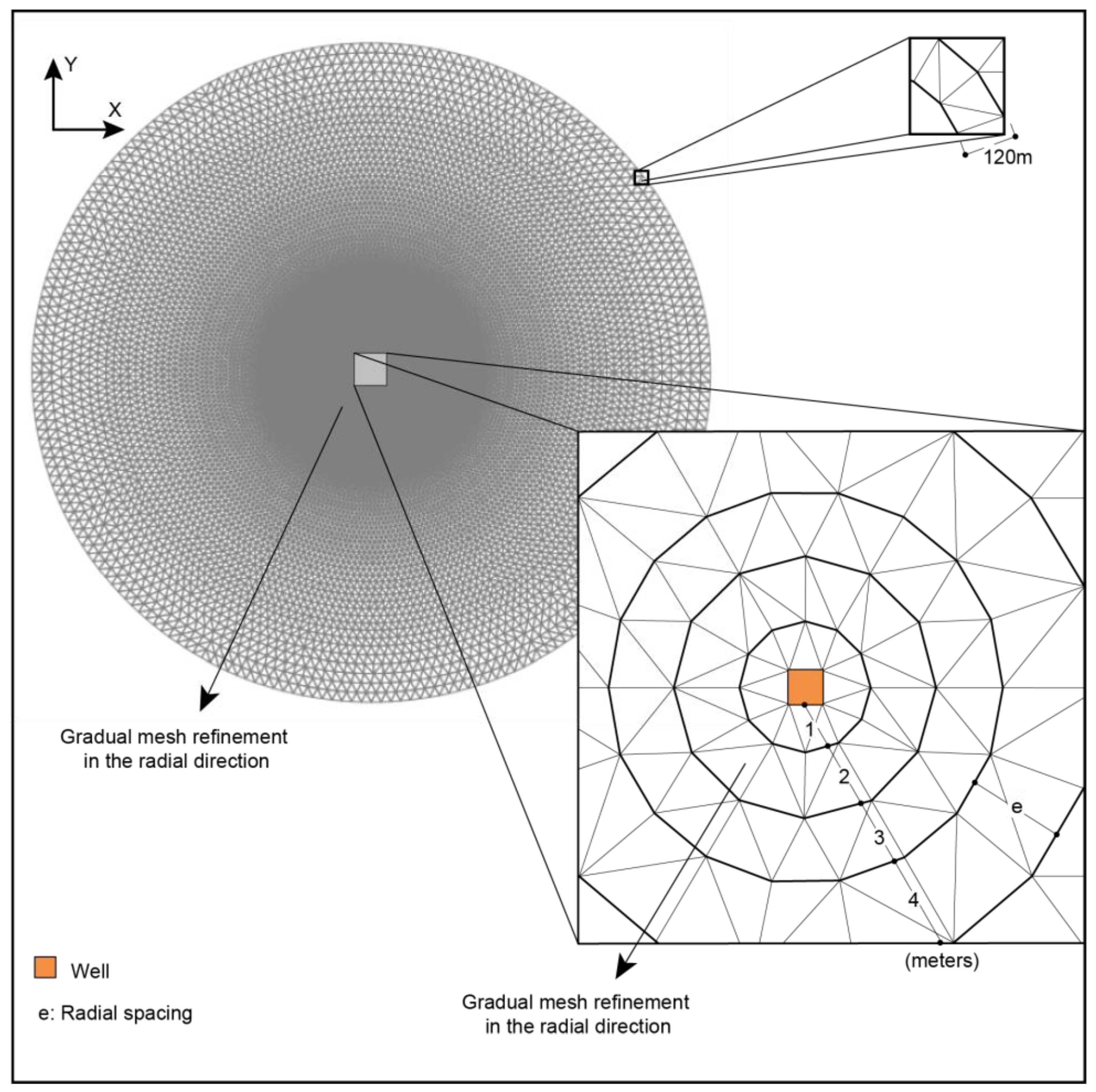
2.1.1. Numerical Model Structural Characteristics

Modeling the water quality extracted during the operation of a managed aquifer recharge (MAR) system in a salinized aquifer required three-dimensional flow simulations with variable density to evaluate the effects of pumping rate, the quality of the freshwater, and the thickness of the aquifer [18,21]. Thus, this method involved creating a base model of a prototype aquifer with an initial salt concentration through three-dimensional numerical flow modeling and describing its main structural and hydrogeological characteristics.

The cylindrical domain represented the unstructured meshes with progressive radial refinement towards the center, forming circular sectors that are subdivided into triangles that decrease in size as they approach the center (Figure 1). At the model’s center, a 1 m square cell contained the extraction well, which spanned the entire aquifer.

2.1.2. Numerical Model Boundary Conditions and Characteristics

In the model, a first-type boundary condition (Dirichlet condition), i.e., the load, was applied to represent the hydraulic head along the lateral walls and the mass sources on the model’s side walls, which remain constant and independent of groundwater flow. These combined conditions represent an infinite mass input to the model through its boundaries.

Additionally, a second-type boundary condition (Neumann condition) was employed at the extraction well located in the central cell, where a specified flow rate was imposed.

2.1.3. Initial Configuration of Aquifer Hydrodynamic Parameters

The assessment of the suitability and effectiveness of the MAR-MASS in transporting mass in aquifers is crucial for sustainable water resource management. Mass in groundwater can result from the natural or anthropogenic dissolution of minerals, the overexploitation of coastal aquifers, saline intrusion, and the discharge of domestic or industrial wastewater. In this context, and in this study, we used 6960 scenarios to assist in building a deep understanding of the underlying dynamics of aquifers, mass transport, and their responses to various hydrogeological conditions.

The transport model considered the parameters of hydraulic conductivity, the vertical anisotropy of hydraulic conductivity, storativity, specific yield, initial salt concentration, molecular diffusion, and mechanical dispersion. The selected values, units, and justifications with the following bibliographical references are presented in

Table 1. Parameters and initial conditions used in numerical simulations.

Parameter	Unit	Set of Selected Values	Justification
Horizontal conductivity (Kh)	m/d	5, 10, 20, 40, 60, 80, 100	Varies from 5 to 100 m/d depending on the geological material [22].
Vertical anisotropy (Kh/Kv)	Dimensionless	1, 10, 20, 30	1 for isotropic aquifers, and other values based on the saltwater intrusion simulation studies [20,23].
Specific storage (Ss)	1/m	1 × 10–5	This value is representative of unconfined aquifers composed of unconsolidated materials, with Kh between 1 and 100 m/d, porosity ranging from 5% to 35%, and thickness varying from 25 to 75 m [24].
Specific yield (Sy)	Dimensionless (%)	15, 20, 25, 30, 35	Sy varies according to the effective porosity—dependent on the type of geological material [25]—and the hydraulic conductivity (see Table 2).
Initial concentration (C)	kg/m3	35, 17.5, 10.5, 7, 3.5	This method considers maximum 35 kg/m3, which is the reference value of seawater, as the initial concentration.
Molecular diffusion coefficient (Dm)	m2/d	0, 0.5702, 1.269	A value of 0 was used for scenarios without molecular diffusion, while the other two values were taken from [26,27].
Longitudinal dispersivity in the horizontal direction (αL)	m	0, 10, 20, 40	This study employs these values to encompass scenarios of average and extreme dispersion within a 7 km domain—interpreted as the diameter in a cylindrical model or the length in a cubic model—based on the equation [28].
Transverse dispersivity in the horizontal direction (αTH)	m	0, 1, 2, 4	αTH is considered 10% of the αL, a typical ratio for this parameter [15,17].
Transverse dispersivity in the vertical direction (αTV)	m	0, 0.1, 0.2, 0.4	This study considers αTV values of 1% of the αL [17].

. The hydraulic heads and mass concentrations in the model were constant and defined through boundary conditions representing the perimeter of the domain area.

Table 2. Specific yield values (S_y) based on material type and hydraulic conductivity (K).

Material			K (m/d)	Sy
				0.15	0.20	0.25	0.30	0.35
Sand and gravel		Medium sand	5	•	•	•	•
			10	•	•	•	•
	Coarse Sand		20	•	•	•	•	•
			40		•	•	•	•
			60		•	•	•	•
			80		•	•	•	•
			100		•	•	•	•

Note(s): Adapted from [22,25]. The symbol “•” indicates combinations of K and Sy values used in the simulation.

shows the specific yield (Sy) values determined using hydraulic conductivity and material classification. Four to five scenarios were used with varying Sy values for each hydraulic conductivity value.

2.2. Numerical Model

2.2.1. Number of Scenarios and Simulations

The set of models analyzed in these studies began with the association of each selected value for the specific yield parameter with the selected values for hydraulic conductivity, resulting in 29 scenarios. In these initial scenarios, four values were selected for mechanical dispersion, three for molecular diffusion, five for salt concentrations in the initial concentration and boundary conditions, and four for vertical anisotropy, resulting in 6960 scenarios.

2.2.2. Temporal Discretization

Temporal discretization determines the time compartments in which the differential equations will solve the phenomena represented in numerical modeling. In the context of salinized aquifers, the MAR-MASS method aims to evaluate the mass removal in the first 2 years of operation and the total mass removal capacity from the aquifer in 5 years, equivalent to 1800 days. The initial tests with temporal discretization of 1, 7, 15, and 30 days resulted in associated mass discrepancies of less than 1%, which were associated exclusively with the model’s hydrodynamic and structural parameters, indicating that the influence of temporal discretization is insignificant.

The results indicated an optimized temporal discretization of 30 days. The 6960 scenarios were simulated for 3000 days, at 30-day intervals, to observe the correlation between extracted mass, hydraulic conductivity, and specific yield.

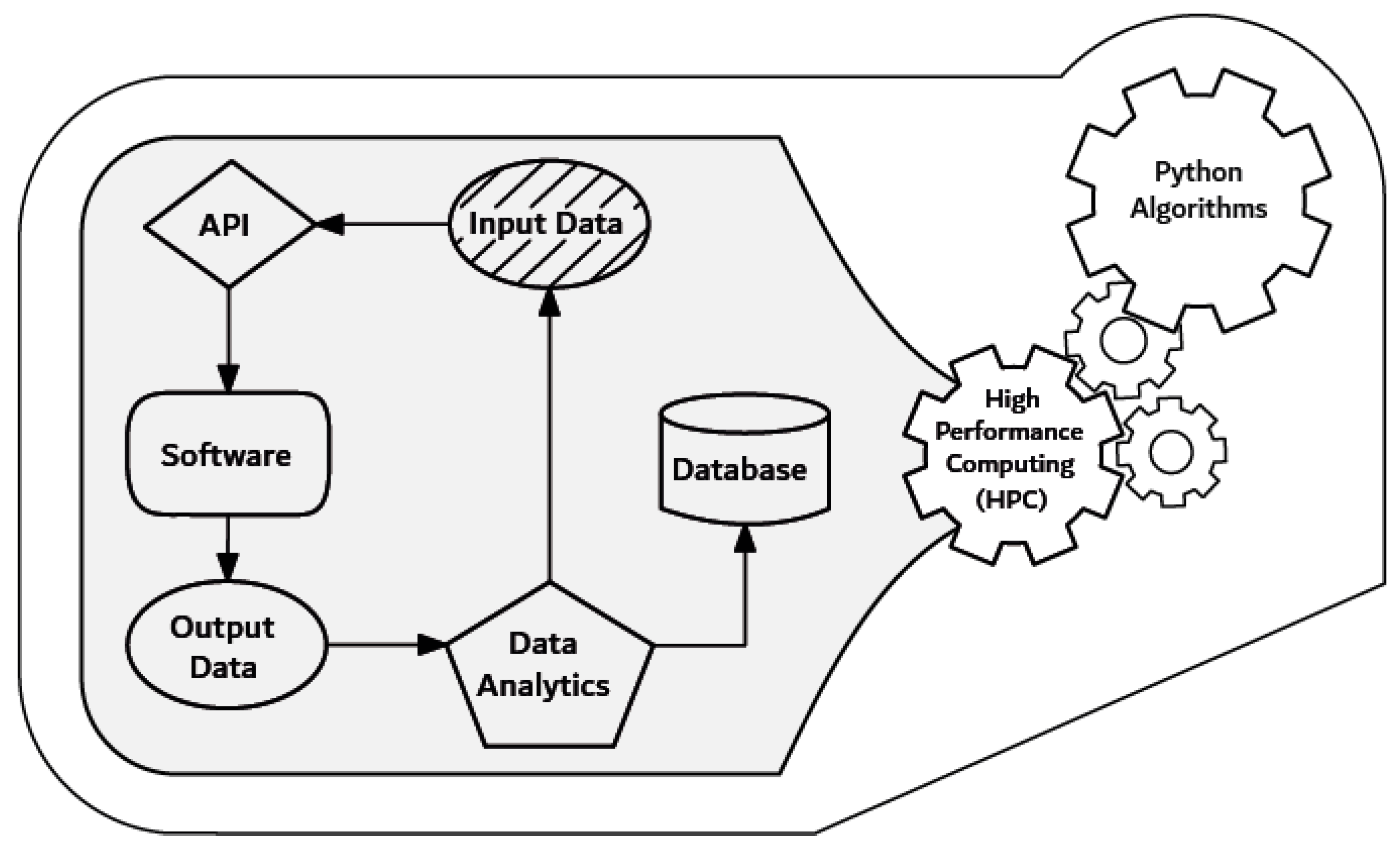
2.2.3. Software Selection, Application Programming Interface (API), and Processors

The selected software packages were MODFLOW 6 and FEFLOW 10, and the application programming interface (API) used was FloPy 3.9.3 for MODFLOW 6 and SEAWAT 4, and IFM 10 for FEFLOW 10. All Python-based scripts were developed using Python 3.13.2. APIs are powerful tools for faster interaction with these software packages through scripts and Python programs. These tools are essential for streamlining the setup processes for the thousands of simulations involved in the MAR-MASS.

Conducting 6960 simulation scenarios through parallel processing requires high-performance computing (HPC). This study used the HPC system resources at the “Centro Nacional de Processamento de Alto Desempenho em São Paulo (CENAPAD-SP)”, with six 128-core processors and 512 GB of memory; here, 6960 simulations were completed in approximately 36 h, making it the selected resource for applying this method.

2.2.4. Workflow

The API processes input data through Python algorithms and fed them into the software. The software performed multiple simulations, storing the results on the workstation. The quality of the results was evaluated based on the criteria of convergence, mass balance, numerical discrepancy, hydraulic gradient, and the drawdown and rise in levels in injection and extraction wells. The redirection of unsatisfactory results to the input dataset restarted the cycle for these models with modifications suggested from a predefined list of options in the algorithm. Finally, the generated information was stored as points that fed into regression, enabling model conditioning, facilitating process interactivity, and reducing the number of simulations required to achieve the objectives. Figure 2 shows the simulation process flow within an HPC system driven by Python algorithms.

The initial objective was to establish a model structure that could meet the hydrogeological conditions required for steady-state flow. An extraction well was simulated in the domain under different flow rates, well screen positions, and varying hydraulic conductivity values. During this phase, the necessary domain extent and depth were determined for each parameter combination, resulting in the geometry of a domain that met a range of solution envelopes. The goal was to create a prototype domain in which the applied boundary conditions would not interfere with the maximum hydraulic gradient generated by the proposed scenarios.

The second step was to validate the MAR-MASS approach through Python algorithms by testing the prototype aquifer. These tests assessed the appropriate injection and extraction well configurations under specific hydrogeological conditions.

The final objective was to statistically analyze the correlation between critical variables, including hydraulic conductivity, specific yield, vertical anisotropy, mechanical dispersion, and molecular diffusion.

2.2.5. Spearman Correlation and Significance Tests

The Spearman correlation coefficient is a non-parametric measure for assessing the rank relationship between two variables. It determines whether there is a monotonic association between the variables, meaning that one tends to increase or decrease as the other does. However, to establish whether the observed relationship is statistically significant, a significance test is necessary to determine whether the correlation coefficient is significantly different from zero [29].

The calculated statistic t approximately follows a Student’s t-distribution when the null hypothesis of no significant relationship is valid. Determining statistical significance involves comparing the calculated t-value with the critical values from the Student’s t-distribution. The p-value associated with this statistic indicates the probability of obtaining a value as extreme or more extreme than the one observed if the null hypothesis was true [30]. If the p-value is less than the established significance level (for example, p < 0.05), then the null hypothesis is rejected, indicating a significant correlation between the variables. Conversely, when the p-value exceeds the significance threshold, insufficient evidence exists for rejecting the null hypothesis. This approach to significance testing is justified by a permutation argument, which asserts that if observations were randomly permuted, then the distribution of correlation coefficients from those permutations would follow a Student’s t-distribution under the null hypothesis of no relationship existing between the variables [31]. This approach justifies the calculated t-value in a dataset as a reliable estimate of the significance of the observed correlation.

To calculate the probability (p) in a two-sided test, this study used the inverse cumulative distribution function of the Student’s t-test [32]. The cumulative probability of the t-distribution is given by Equation (1):

$$p=P\left(T\ge \left|t\right|\right)$$

(1)

where $P\left(T\ge \left|t\right|\right)$ represents the probability that the observed value of t is greater than or equal to the absolute value of t under the Student’s t-distribution with the specified degrees of freedom; T is the variable that follows a Student’s t-distribution; and t is the Student’s t-distribution with n − 2 degrees of freedom under the null hypothesis.

Using the t-statistic and the degrees of freedom (n − 2), one can calculate the probability value with functions available in software like Excel, specifically the T.DIST.2T (t, n − 2) function. If the p-value was less than 0.05, then the null hypothesis was rejected, and we concluded that there was a significant correlation between the variables.

3. Results

The 6960 proposed scenarios provided a comprehensive framework for analyzing the interaction between critical variables, including hydraulic conductivity, specific yield, vertical anisotropy, mechanical dispersion, and molecular diffusion. This analysis identified behavior patterns when implementing the method, such as the amount of extracted mass, the extraction efficiency, the propagation of injected freshwater, the residual concentration in the intervention area at the end of the peak efficiency period, and the system’s operation time for each scenario to remove the mass from the intervention area until a residual concentration that is safe for drinking was reached.

3.1. Amount of Mass Extracted for a Simulation Period of 3000 Days for the Injection Extraction Scenario

At the end of 3000 simulation days, a correlation was observed between the extracted mass, hydraulic conductivity, and specific yield when analyzed. The Spearman correlation coefficient was used in this analysis to measure the strength and direction of the relationship between the different variables.

Table 3. Spearman values for extracted mass with different initial concentrations at the end of 3000 simulation days.

Parameter	All Data	Initial Concentration (kg/m3)
		35.0	17.5	10.5	7.0	3.5
Initial concentration	0.95
K	0.21	0.86	0.79	0.71	0.64	0.58
Sy	0.25	0.61	0.72	0.80	0.86	0.91
Mechanical Dispersion	0.03	0.04	0.06	0.07	0.08	0.08
Molecular Diffusion	0.02	−0.14	−0.04	0.04	0.1	0.16
Anisotropy	−0.04	−0.18	−0.19	−0.19	−0.16	−0.07

summarizes the correlation coefficient results for all parameters at all initial concentrations and for concentrations of 35, 17.5, 10.5, 7, and 3.5 kg/m³. When examining the behavior of mass extraction with these parameters, a clear and prominent correlation emerged. This correlation was identified as the relationship between mass extraction and the initial concentration of the medium, observed consistently across all initial concentration data, with a correlation coefficient of 0.95. This value indicated a direct association between the initial concentration and the extracted mass, suggesting that as the initial concentration rises, so does the mass extracted, although this does not necessarily occur in a proportional manner. In addition to the initial concentration, hydraulic conductivity and specific yield were significant factors in mass extraction.

Specific yield refers to a fraction of the volume of water that can be naturally released from the aquifer. Four to five Sy scenarios were simulated for each hydraulic conductivity value (Table 2), suggesting a correlation between hydraulic conductivity and specific yield (Table 3). Increasing the volume of water extraction resulted in a greater mass being removed from the aquifer. The amount of mass extracted was proportional to the solute concentration in the water.

A positive Spearman correlation coefficient between the extracted mass and hydraulic conductivity indicated a direct relationship with the amount of mass extracted. Table 3 suggests that as the initial concentration increased, the correlation between hydraulic conductivity and the amount of mass extracted also increased. For an initial concentration of 35 kg/m³, the Spearman correlation coefficient for hydraulic conductivity was 0.86, indicating a moderately strong positive correlation between the initial concentration, extracted mass, and hydraulic conductivity. The correlation coefficients indicated weaker positive correlations as the initial concentration decreased, diminishing the importance of hydraulic conductivity concerning the extracted mass.

An inverse phenomenon to hydraulic conductivity occurred in the case of specific yield. For an initial concentration of 35 kg/m³, the correlation coefficient was 0.61, showing a moderate positive correlation. As the initial concentration decreased, the correlation increased to a strong positive correlation between the extracted mass and the specific yield, with a value of 0.91 for an initial concentration of 3.5 kg per cubic meter (Table 3).

Vertical anisotropy, mechanical dispersion, and molecular diffusion exhibited small values with minor fluctuations, making correlation coefficients unreliable as a statistical analysis tool for these parameters (Table 3). For mechanical dispersion and molecular diffusion, Spearman correlation coefficients remained relatively low across all concentrations (≤0.16; Table 3). However, significance testing (

Table 4. Significance test summary from Spearman values.

Parameter	All Data	Initial Concentration (kg/m3)
		35.0	17.5	10.5	7.0	3.5
Initial concentration	0
K	4 × 10−70	0	0	0	0	0
Sy	1 × 10−99	0	0	0	0	0
Mechanical Dispersion	0.012	0.14 **	0.025	0.009	0.003	0.003
Molecular Diffusion	0.095 **	2 × 10−7	0.14 **	0.14 **	2 × 10−4	2 × 10−9
Anisotropy	8 × 10−4	1 × 10−11	9 × 10−13	9 × 10−13	2 × 10−9	0.009

Note(s): ** Bold values indicate p > 0.05 (not statistically significant).

) revealed that in specific concentration subsets, namely, ≤17.5 kg/m³ for mechanical dispersion and ≤7 kg/m³ for molecular diffusion, the p-values fell below 0.05. This indicated that, despite their low magnitude, these correlations were statistically significant, suggesting that even subtle variations in dispersion and diffusion can meaningfully affect mass extraction under certain hydrodynamic conditions. Vertical anisotropy exhibited consistently negative Spearman values (from −0.07 to −0.19, Table 3), suggesting that higher anisotropy tended to reduce mass extraction efficiency. Despite the low magnitude of the Spearman values, the p-values were statistically significant (p < 0.01 across all concentrations, Table 4), reinforcing the reliability of this trend. These results indicated that vertical anisotropy, while exerting a minor effect compared to hydraulic conductivity and specific yield, plays a significant role in mass transport dynamics within the MAR-MASS method.

Table 4 presents the significance values (p-values), which are the t-Student values that were previously calculated. The t-Student calculations used the Spearman values in Table 3, with 6950 observed values (n) for the entire dataset and 1390 for each initial concentration. Values less than 1 × 10⁻¹⁰⁰ were recorded as zero in the table. A p-value greater than 0.05 indicates insufficient evidence to reject the null hypothesis, meaning the correlation between the variables is not statistically significant at the 5% significance level. Conversely, p-values below 0.05 support rejecting the null hypothesis, suggesting that the observed correlation is statistically significant, even if its magnitude is low.

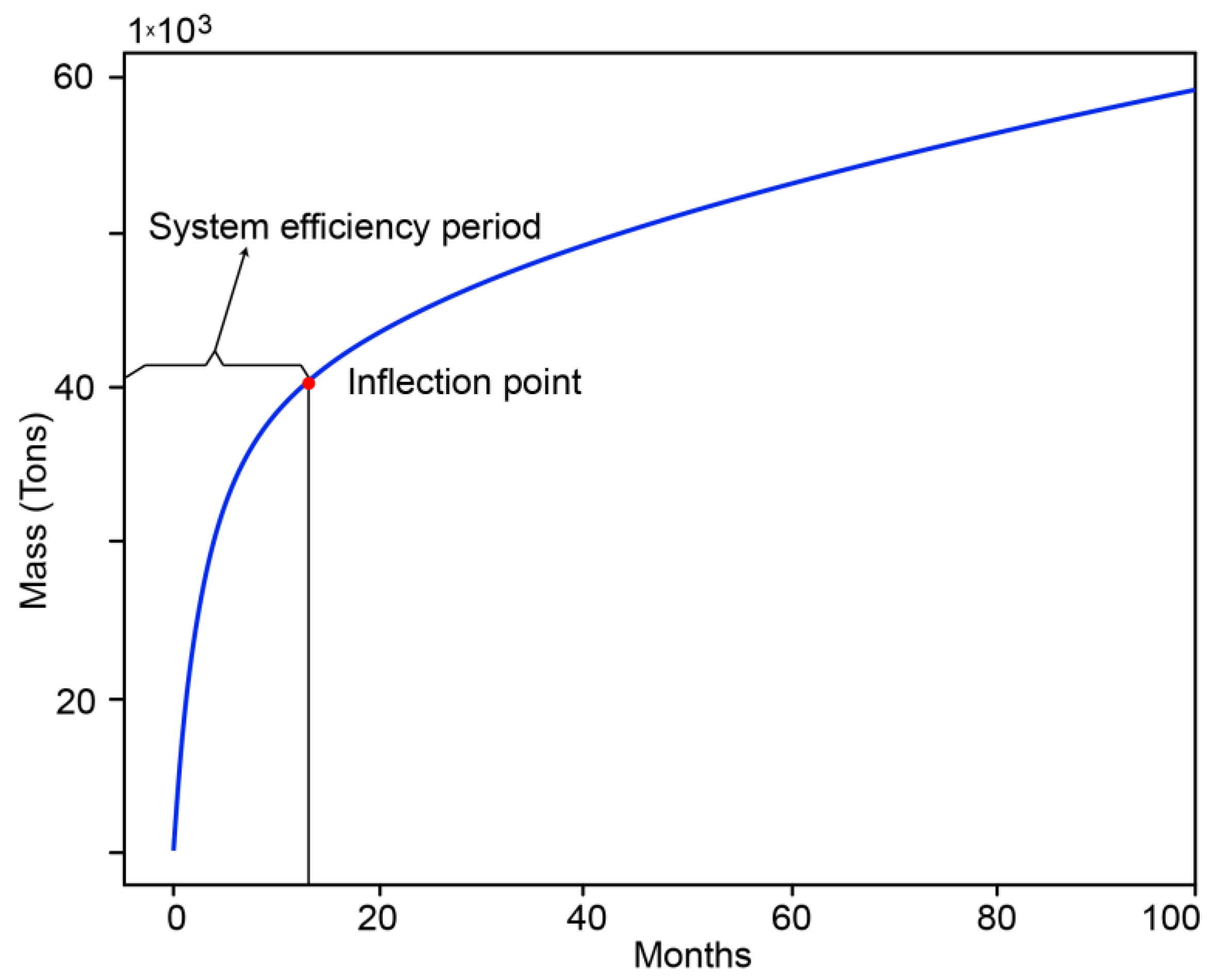
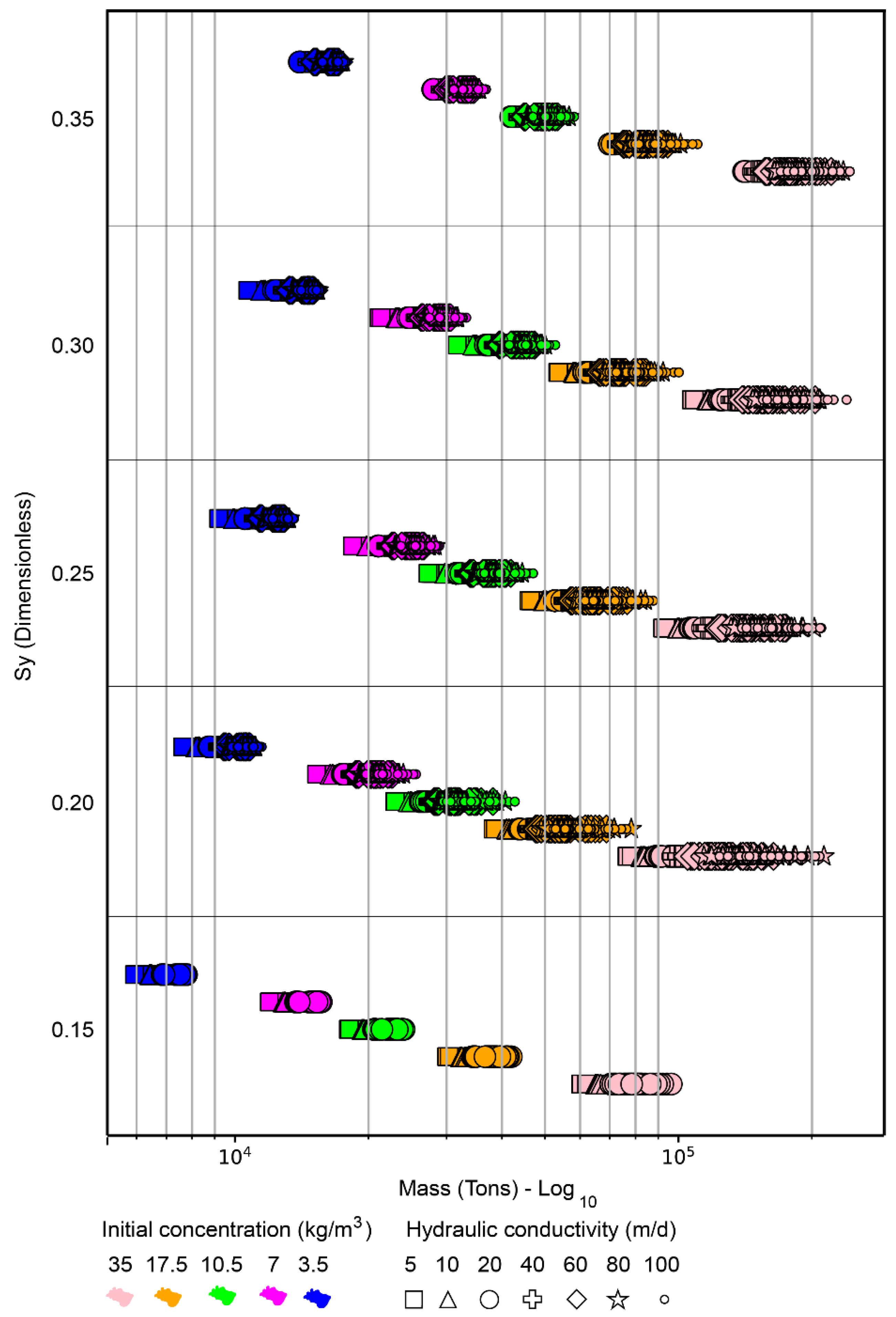
3.2. System Efficiency Period and Mass Extraction Values According to the Parameters Analyzed

A direct correlation existed between Sy and mass extraction in the aquifer, as evidenced in the simulations. However, this relationship is not universally consistent, since the extracted mass is influenced by multiple interacting factors beyond Sy and the initial concentration, such as hydraulic conductivity, vertical anisotropy, mechanical dispersion, and molecular diffusion. To better analyze this behavior, it is useful to reference when mass extraction in the system loses efficiency.

Figure 3 illustrates an example of this behavior among the 6970 simulated scenarios, representing a 50 m thick aquifer with an initial concentration of 10.5 kg/m³, a hydraulic conductivity of 20 m/d, 30% specific yield, 10% vertical anisotropy, 10 m longitudinal dispersivity, and a molecular diffusion coefficient of 0.5703 m²/d. The system was more efficient up to 14 months, which marked the inflection point. This value was determined mathematically using the Python library KneeLocator. The code tested different combinations of configurations, analyzed the fitted curve, and calculated the point where the second derivative was most pronounced, indicating the highest relative curvature.

The efficiency period and the mass extracted during this period varied according to the initial concentrations and the mentioned hydrodynamic parameters. The correlation between the specific yield, the initial concentration, and the mass extracted was evident during this system efficiency period. According to

Table 5. Spearman correlation values for the extracted mass at different initial concentrations in all scenarios during the efficiency period.

Parameter	All Data	Initial Concentration (kg/m3)
		35.0	17.5	10.5	7.0	3.5
Initial concentration	0.95
K	0.18	0.80	0.65	0.59	0.57	0.57
Sy	0.27	0.73	0.87	0.91	0.92	0.93
Mechanical Dispersion	−0.04	−0.15	−0.14	−0.15	−0.15	−0.15
Molecular Diffusion	−0.01	0.00	0.03	0.03	0.03	0.03
Anisotropy	−0.01	−0.13	−0.12	−0.08	−0.04	0.00

, the level of correlation increased for specific yield and initial concentration compared to Table 3 at the end of 3000 simulation days. For each initial concentration, the correlation levels for specific yield became more pronounced than those for hydraulic conductivity as the initial concentrations decreased.

Table 6. Significance test summary from data presented in Table 5.

Parameter	All Data	Initial Concentration (kg/m3)
		35.0	17.5	10.5	7.0	3.5
Initial concentration	0
K	1 × 10−51	0	0	0	0	0
Sy	0	0	0	0	0	0
Mechanical Dispersion	8 × 10−4	2 × 10−8	2 × 10−7	2 × 10−8	2 × 10−8	2 × 10−8
Molecular Diffusion	0.4 **	1 **	0.26 **	0.26 **	0.26 **	0.26 **
Anisotropy	0.4 **	1 × 10−6	7 × 10−6	0.003	0.14 **	1 **

Note(s): ** Bold values indicate p > 0.05 (not statistically significant).

highlights the correlation between the extracted mass during the efficiency period and parameters such as vertical anisotropy, mechanical dispersion, and molecular diffusion, which remained very low compared to hydraulic conductivity and specific yield. Mechanical dispersion exhibited consistently low Spearman correlation coefficients across all concentration levels (Table 5); however, these correlations were statistically significant (p < 0.001, Table 6). In contrast, molecular diffusion showed high p-values (p > 0.05), indicating no statistically significant correlation during the efficiency period. Vertical anisotropy presented low-magnitude correlation coefficients but statistically significant p-values at higher initial concentrations (10.5 to 35.0 kg/m³), suggesting that even subtle relationships may influence mass extraction under specific conditions. The calculations of the significance values (p-values) in Table 6 followed the MAR-MASS approach, as outlined in Table 4, using the values provided in Table 5 and treating p-values below 1 × 10⁻¹⁰⁰ as zero.

The mass extracted during the peak efficiency period showed a strong correlation with the initial concentration in a general sense across all evaluated scenarios. For aquifers with a thickness of 50 m, it was possible to estimate the probable maximum and minimum ranges of the mass extracted during this period, considering variations in specific yield and initial concentration. Figure 4 shows that the accumulated mass extracted in the system was directly proportional to the concentration. For instance, a specific yield of 30% and a concentration of 3.5 kg/m³ resulted in an accumulated mass of approximately 16,000 tons. The mass extracted was ten times greater at 35 kg/m³. The extracted mass gradually increased with a higher specific yield. Additionally, as the initial concentration rose, the influence of hydraulic conductivity became more pronounced, accelerating transport and enhancing the total mass recovered, as shown in Figure 4.

Longitudinal dispersion may directly relate to mechanical dispersion through specific dispersion parameters, considering the porous medium’s heterogeneity. These parameters may include longitudinal and transverse dispersivities, which measure the extent of dispersion in the direction of flow and perpendicular to the flow, respectively. Hydrogeological modeling software such as MODFLOW 6, SEAWAT 4, and FEFLOW 10 can incorporate this direct relationship between mechanical and longitudinal dispersion in their calculations. Mechanical dispersion affects longitudinal dispersion through spatial variations in flow velocity that promote solute mixing and transport. When the porous medium presents significant heterogeneity, mechanical dispersion increases, leading to greater longitudinal dispersion of contaminants. While one might assume that such dispersion improves remediation by increasing the area in which contaminants interact with extraction zones, the results indicated the opposite. Greater mechanical dispersion, especially at higher concentrations, hindered effective mass extraction. This was not only a visual trend in Figure 5, but a clear quantitative result supported by Table 5, which shows a negative correlation between longitudinal dispersivity and the extracted mass. This suggested that increased dispersion promotes dilution and spatial dispersion, ultimately reducing the mass of contaminants available for recovery at a given location.

The MAR-MASS method aimed to efficiently extract the mass in the aquifer using injection and extraction flow rates, which, according to the method, increased according to hydraulic conductivity. As observed in Figure 6, the increase in conductivity provided a more extended period of efficiency in mass extraction, which was accentuated in the presence of higher mass concentrations in the aquifer. Increasing the specific yield in hydraulic conductivities from 5 to 20 m/d could extend the period of mass extraction efficiency, which, based on the injected and extracted flow rates, enables mass extraction at greater distances in the presence of higher specific yield values. However, for conductivities of 40 to 100 m/d, where higher flow rates were implied than those used for conductivities of 5 to 20 m/d, the increase in specific yield led to a decrease in efficiency time due to the more rapid depletion of available mass in the storage within the intervened zone, which became more noticeable at higher aquifer concentrations. The estimated efficiency period for mass extraction for initial concentrations between 3.5 and 17.5 kg/m³ ranged from 420 to 480 days for 90% of the scenarios proposed, while this efficiency period was only possible in 60% of scenarios with an initial concentration of 35.0 kg/m³.

3.3. Propagation of Fresh Water Injected Within the Proposed Method’s Efficiency Period

After implementing the MAR-MASS approach, understanding the mass distribution within the intervention area is crucial for evaluating its efficiency. Residual concentration refers to the dissolved mass in the groundwater within the intervention area after the method’s implementation. Analyzing this concentration at the end of the maximum efficiency period for mass extraction in each proposed scenario revealed a strong correlation with the aquifer’s initial concentration (Figure 7). The decrease in residual concentration in the intervention area for each concentration was, in turn, associated with the increase in hydraulic conductivity. For the same concentration, a slight increase in residual concentrations was observed as the specific yield increased, and it was noticeable when the hydraulic conductivity decreased, indicating that mass transport continues to be influenced by the specific yield. Analyzing the minimum residual values for each concentration revealed no appreciable change for different specific yield values, allowing us to infer that all the mass present in the storage that could be removed reached its maximum threshold in this period of maximum efficiency according to the adopted configuration. Values lower than these minimums and maximums could be achieved by reducing the distance between wells or increasing the intervention time, knowing that the extraction of mass would be less efficient but still significant with the application of the method. The method could have several objectives motivating the extraction of mass in an aquifer; one could be extracting mass to the point where the intervention area reaches potability with a concentration of 0.5 kg/m³, as suggested by the National Secondary Drinking Water Regulations of the Environmental Protection Agency [33]. Pursuing this objective would mean that for initial concentrations of 3.5 to 17.5 kg/m³, 92% of the proposed scenarios would achieve potability within the maximum efficiency period. Achieving potability within a period equal to or less than 480 days was possible for these scenarios. For scenarios with initial concentrations of 35 kg/m³, only 14% of the scenarios would fall within the potability range, and the highest residual concentration value reached in that efficiency period would be 2.8 kg/m³, representing a maximum value equivalent to 8% of the initial concentration.

The influence of mechanical dispersion on the residual concentration at the end of the maximum efficiency period was significant. In Figure 8, for each initial concentration, it can be seen that for the condition where mechanical dispersion was not considered, the minimum values can be up to ten times lower than the maximum values when considering the highest longitudinal dispersion value; 90% of scenarios with zero mechanical dispersion would reach the potability range at the end of the maximum efficiency period, while 71% achieved this when considering a longitudinal dispersion of 40 m. When molecular diffusion was zero, its impact represented only a 5% increase in cases that would reach potability under conditions of zero mechanical dispersion.

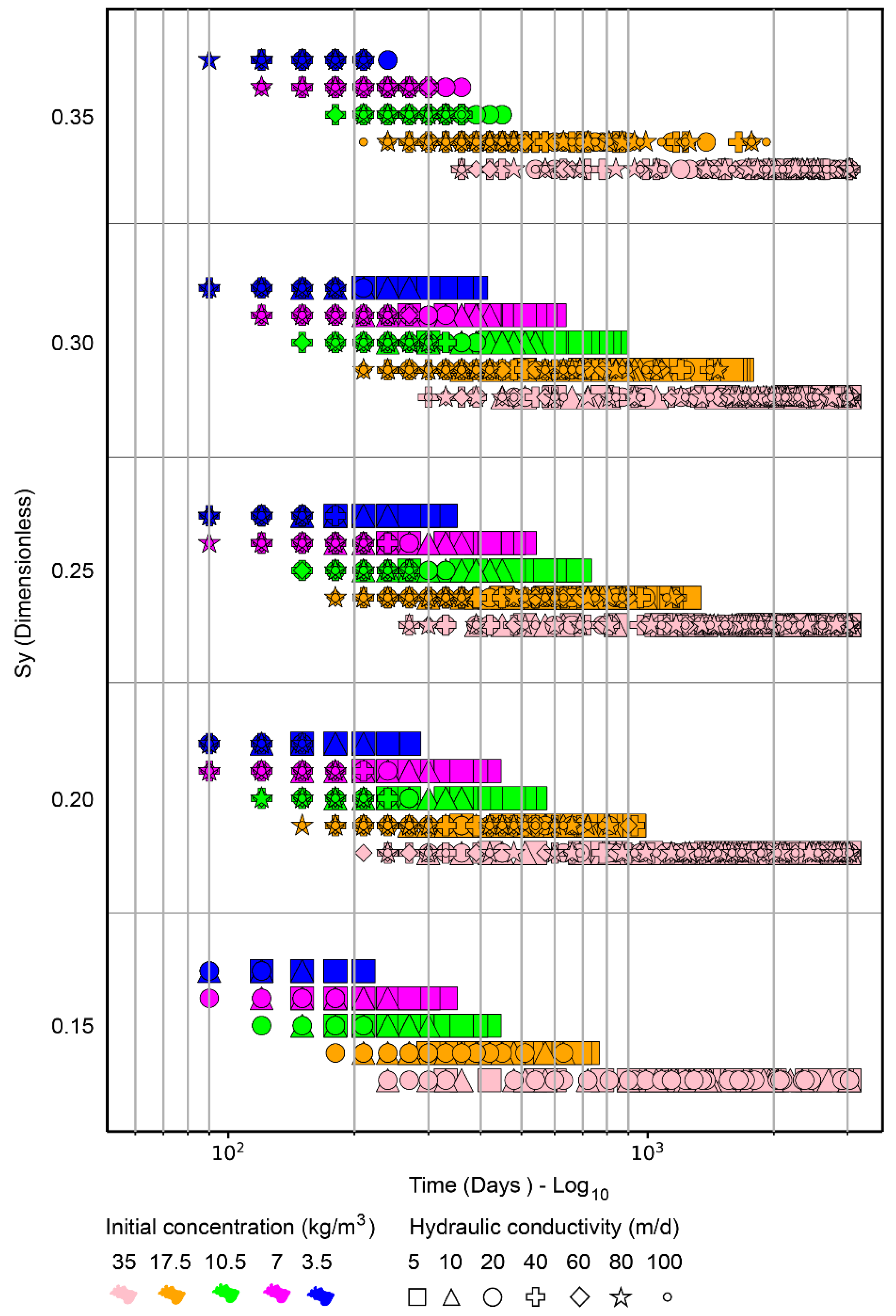
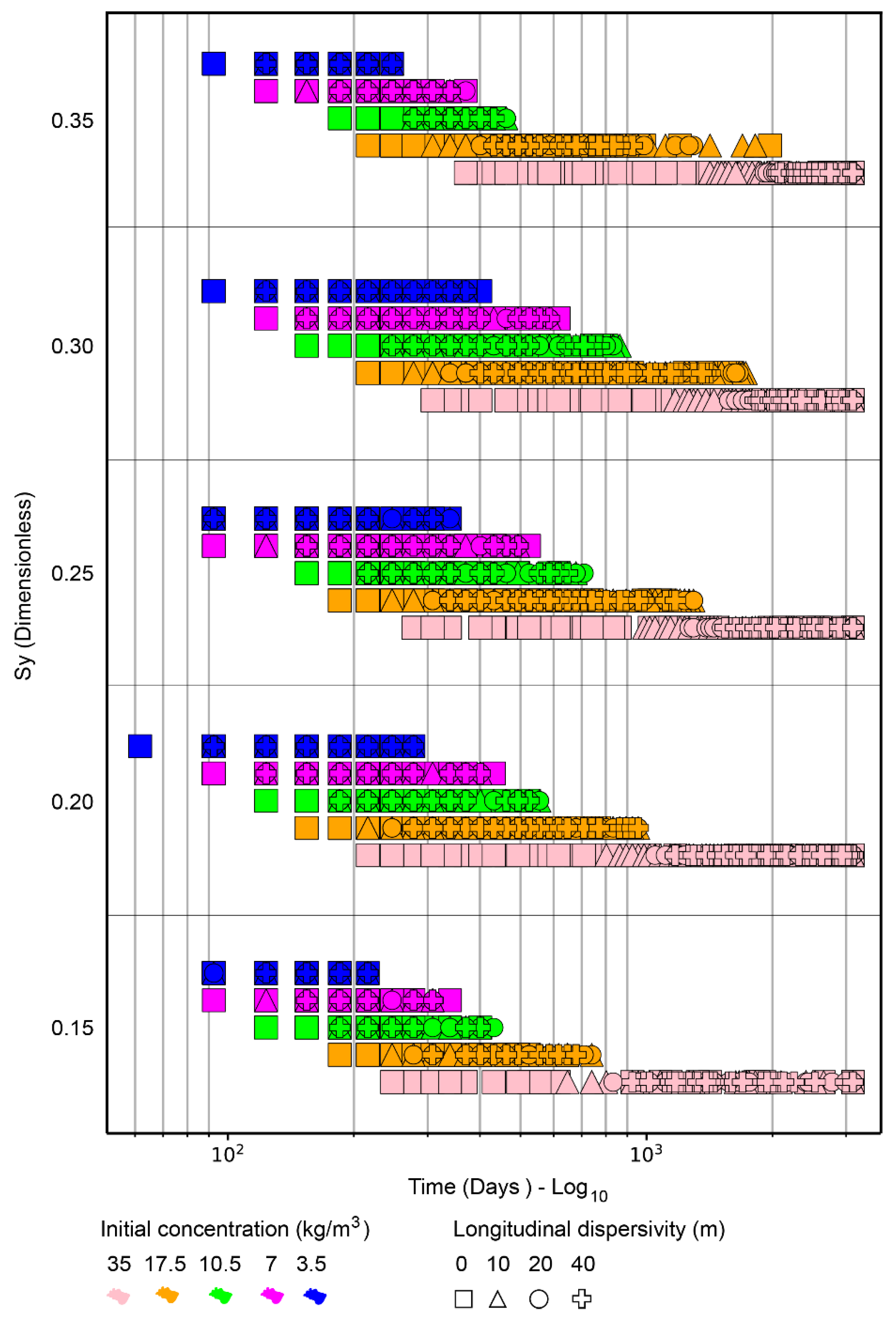
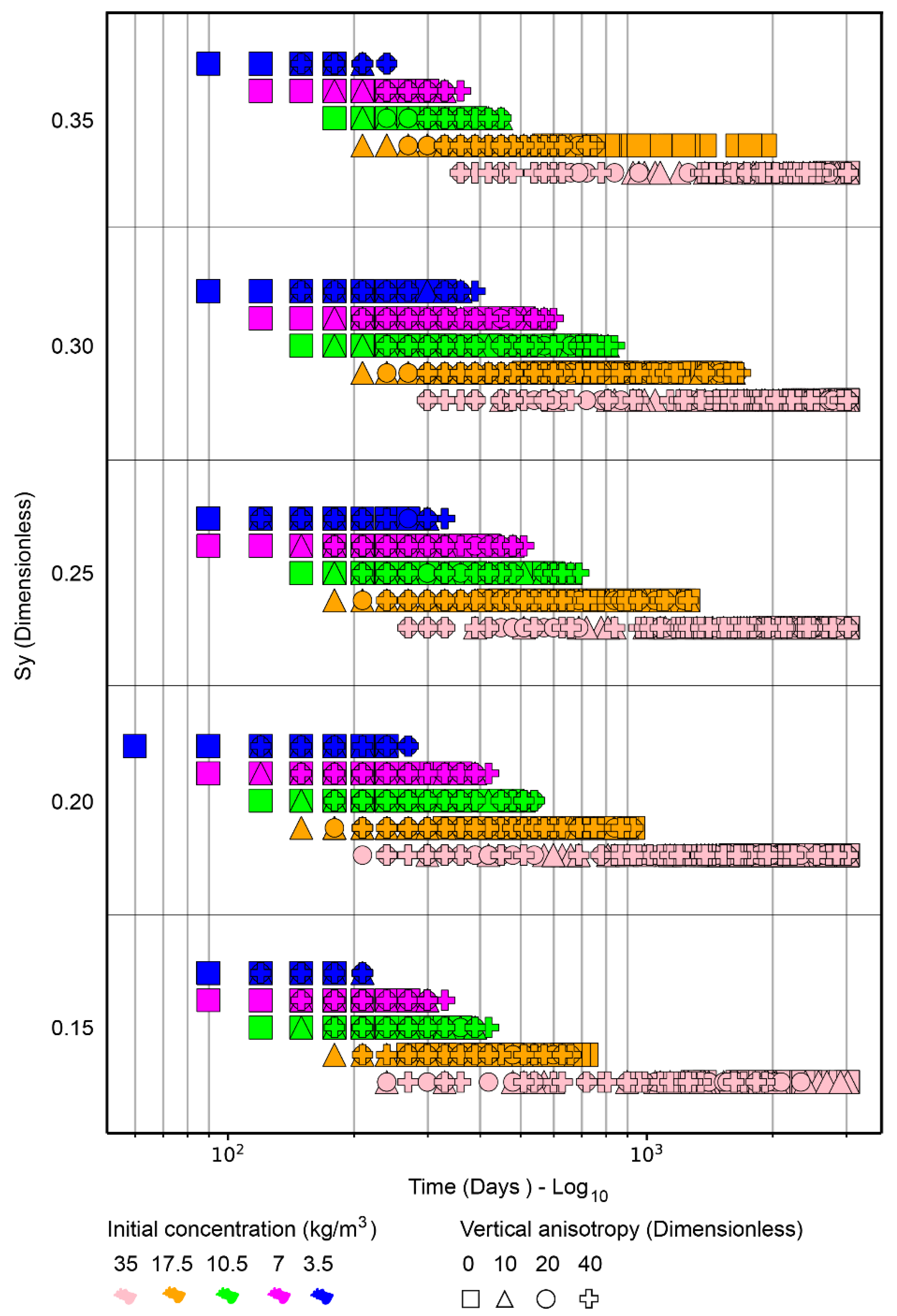
3.4. System Operation Time to Purify Salinized Areas Until Reaching Safe Levels for Drinking Water Consumption

The MAR-MASS method could be designed to achieve target outcomes, such as mass removal, until specific residual concentrations are reached. A goal could be to attain a residual concentration for aquifer remediation to the extent that the water stored in the aquifer is safe for drinking, at least under certain salinity conditions.

Up to 3000 days of simulation were carried out to analyze the behavior of the proposed scenarios beyond the maximum efficiency period and calculate the time it would take for each scenario to reach a target residual concentration of 0.5 kg/m³. During this extended time, the effect of hydraulic conductivity on the days when potabilization is achieved could be observed. Figure 9 shows that for initial concentrations from 3.5 to 10.5 kg/m³, there was a reduction in the number of days as the hydraulic conductivity increased, partly influenced by the increase in the extraction and injection flow in the method. However, this effect weakened at a concentration of 17.5 kg/m³ and was imperceptible for the 35.0 kg/m³ concentration, highlighting a strong correlation between the initial aquifer concentrations and mass displacement. Figure 9 reveals several findings regarding the transport of mass for different hydraulic conductivities. On a logarithmic scale, the time required to achieve potabilization became evident. Analyzing the time associated with each initial concentration revealed a consistent pattern. One can observe that although there was a fivefold difference in concentrations, such as 3.5 and 17.5 kg/m³, for specific yields less than 0.3, this proportion needed to be reflected in the number of days required to achieve potabilization at these concentrations. When observing initial concentrations from 3.5 to 17.5 kg/m³ individually, concerning the specific yield, an increase in the number of days for potabilization was noted. This increase maintained a linear pattern seen from a logarithmic scale for specific yields less than or equal to 0.3. For specific yields equal to 0.35, which is a high yield value, there was a significant reduction in the number of days taken to achieve potabilization for the proposed scenarios due to the accelerated depletion of the mass in storage in the intervention area. For all specific yield values, there were 1880 scenarios where potabilization could be achieved in a short period between 90 and 120 days. However, scenarios where the specific yield was 0.3 could be considered to be the most critical. More challenging potabilization time ranges could be estimated in this set of scenarios. For initial concentrations of 3.5 kg/m³, potabilization could be achieved in a maximum time of 390 days; for 7 kg/m³, the maximum time would be 600 days; for 10.5 kg/m³, the maximum time would be 840 days; and for 17.5 kg/m³, the maximum time would be 1920 days. For initial concentrations of 35 kg/m³, 33% of the scenarios did not achieve potabilization within 3000 days, ending with an average residual concentration in these scenarios of 0.64 kg/m³. This method was designed to facilitate efficient mass extraction for 1 to 5 years. As depicted in Figure 6, 92% of these scenarios accomplished this within a time frame equal to or less than 480 days. However, under stricter potabilization conditions for the adopted configuration, 62% of the scenarios achieved it within a year, while 17% did so in the second year. Between the second and third years, the proportion of scenarios meeting the more stringent potability criteria decreased sharply to 4%; by the fourth year, this percentage further declined to 3%, and by the fifth year, only 2% of the scenarios achieved this condition. Overall, 88% of the scenarios reached potabilization within five years, with 79% doing so within the first two years. Due to the scalability and adaptability of the method, a reduction in the potabilization time in the most critical scenarios could be achieved solely by reducing the spacing of the wells.

Mechanical dispersion influences the critical scenarios in terms of mass extraction. According to Figure 10, the correlation between mechanical dispersion and the time required for a scenario to reach a residual concentration of 0.5 kg/m³ became stronger as the initial concentration increased. This phenomenon, produced by mechanical dispersion, became more noticeable at the concentration of 35 kg/m³, with its effect increasing linearly with specific yield when analyzed on a logarithmic scale.

The influence of vertical anisotropy on the potabilization time depends on its interaction with other hydrogeological parameters. Although Table 5 shows a weak negative correlation between vertical anisotropy and extracted mass, particularly at higher initial concentrations, this effect was not consistently observed across all scenarios and was not statistically significant for initial concentrations equal to or below 7.5 kg/m³ (Table 6). Likewise, while vertical anisotropy can influence mass displacement within the aquifer, especially in deeper zones, its impact on the time required to reach potable concentrations (0.5 kg/m³) was less evident at initial concentrations above 10.5 kg/m³ (Figure 11).

4. Discussion

For an extended simulation period, high hydraulic conductivity values were associated with a greater volume of extracted salt mass when linked to high initial concentrations, as expected. However, this increase in mass was not proportional to hydraulic conductivity. During the peak efficiency period, the increase in extracted mass was slightly related to hydraulic conductivity for initial concentrations between 3.5 and 10.5 kg/m³, and the influence of hydraulic conductivity became significant for initial concentrations starting from 17.5 kg/m³. The period of maximum efficiency extended with higher conductivity due to the flow increase configuration as conductivity rose in the method. This efficiency time increase was more pronounced for initial concentrations of 17.5 and 35 kg/m³ and hydraulic conductivities between 40 and 100 m/day. This depended on the specific performance since lower specific yield values led to a more significant time to reach equilibrium. The residual concentration in the intervention area at the end of the peak efficiency period decreased as hydraulic conductivity increased. The time required to reach a residual concentration of 0.5 kg/m³ notably decreased with increasing hydraulic conductivity for concentrations between 3.5 and 10.5 kg/m². However, this effect weakened at an initial concentration of 17.5 kg/m³ and was imperceptible for 35 kg/m³. Analyzing the specific yield over an extended simulation period revealed a strong influence of specific yield on the extracted mass in the presence of initial concentrations between 3.5 and 10.5 kg/m³, diminishing for higher concentrations. When specific yield was analyzed during the peak efficiency period, a gradual increase in extracted mass was observed as specific yield rose. The peak efficiency time slightly increased with a higher specific yield for initial concentrations between 3.5 and 10.5 kg/m³ and a hydraulic conductivity of 5 to 20 m/day. The residual concentration at the end of the peak efficiency period gradually increased with higher specific yield, and this increase was more pronounced as hydraulic conductivity values decreased. As specific yield increased, there was also a gradual increase in the time required to reach a residual concentration of 0.5 kg/m³.

Vertical anisotropy plays a significant role in mass displacement from one point to another, which was particularly noticeable with initial concentrations above 10.5 kg/m³. This displacement effect may be more evident at the aquifer base and could influence the desalination time in that zone. However, when considering mass extraction across the intervention area, no identifiable pattern of vertical anisotropy emerged; this was due to hydraulic conductivity and specific yield exerting more significant influences on mass extraction, followed by mechanical dispersion. The extracted mass values could be similar for different vertical anisotropies when evaluating the combinations of hydraulic conductivity and specific yield values. Potential coincidences in these results could increase when involving different mechanical dispersion values.

On the other hand, increased mechanical dispersion led to a decrease in the extracted mass during the peak efficiency period in most cases. This effect was noticeable when observing the residual concentration at the end of the peak efficiency period, where differences of up to 10 times in residual concentration values could be observed for a longitudinal dispersion coefficient of 40 m compared to scenarios without mechanical dispersion. Consequently, increased mechanical dispersion led to more days being taken to reach a target residual concentration of 0.5 kg/m³. Although molecular diffusion barely influenced mass extraction through the method, scenarios lacking diffusion formed part of the 5% group of cases achieving a target residual concentration of 0.5 kg/m³ by the end of the efficiency period.

From an operational perspective, the proposed MAR-MASS method provides practical benefits for groundwater remediation in complex aquifer systems. This approach enhances control over the hydraulic front and improves efficiency in environments that are heterogeneous or have low permeability. Such conditions often cause traditional pump-and-treat methods to underperform [11,15]. By optimizing flow distribution, it reduces resistance in deeper zones and facilitates the upward migration of fresher water. Its modular and scalable design allows it to adapt to areas of interest efficiently. As a result, remediation times are shortened, and the overall effectiveness of the process increases.

Furthermore, the MAR-MASS method enables a more precise design of pumping configurations by identifying the threshold values of key parameters such as hydraulic conductivity and specific yield. It also allows for better allocation of resources. Additionally, the limited influence of certain parameters, such as molecular diffusion and vertical anisotropy, in specific scenarios suggests that the complexity of the conceptual and numerical model can be reduced without compromising accuracy.

Importantly, reducing the operational duration and energy consumption directly contributes to lowering the carbon footprint of remediation activities. This aspect makes the MAR-MASS method particularly relevant in projects focused on sustainability, where energy efficiency and climate considerations are critical [16,34]. Nevertheless, it is essential to recognize that current results are based on numerical simulations. Therefore, applying the MAR-MASS method in real-world situations requires field validation. Such validation must account for site-specific hydrogeological conditions, infrastructure constraints, and long-term system behavior to ensure that the actual performance aligns with the predicted outcomes.

5. Conclusions

During an extended simulation analysis, the effects of hydraulic conductivity were noticeable when evaluating the period of maximum mass extraction efficiency. For initial concentrations below 17.5 kg/m³, the amount of mass extracted showed greater sensitivity to hydraulic conductivity than at higher concentrations. Furthermore, the time required to reach potability in the intervention area was shorter for initial concentrations below 17.5 kg/m³ and was influenced by the increase in hydraulic conductivity. The effect of hydraulic conductivity was inconclusive when evaluating initial concentrations of 35 kg/m³.

The specific yield effect on extracted mass is highly relevant; however, this effect was more pronounced for initial concentrations below 17.5 kg/m³ and hydraulic conductivities less than or equal to 20 m/d. The increased significance of this effect can be attributed to the system configuration applied in the method. The analysis did not reveal a consistent relationship between the variation in vertical anisotropy and the total mass extracted during 3000 simulated days. An increase in mechanical dispersion enhanced the mass extraction efficiency but also extended the time required to reach the desired residual concentrations. In applying the method, vertical anisotropy did not exert dominant control over the system performance at initial concentrations above 10.5 kg/m³; its effects were attenuated by the more prominent influence of hydraulic conductivity and specific yield. Molecular diffusion had a minimal effect on the extraction process. Understanding these influences is imperative in enhancing extraction procedures and efficiently attaining the desired concentration levels.

From a practical perspective, these findings provide valuable guidance for stakeholders engaged in groundwater quality restoration. Identifying the optimal hydrogeological conditions for efficient mass extraction supports the strategic planning of well placement, pumping rates, and anticipated remediation timelines. Furthermore, by highlighting which parameters critically influence system behavior and which have a lesser impact, this study contributes to the development of more targeted and cost-effective approaches for managing salinized groundwater systems.

References

1. Gorelick, S.M.; Zheng, C. Global change and the groundwater management challenge. Water Resour. Res. 2015, 51, 3031–3051. [Google Scholar] [CrossRef]
2. Calvin, K.; Dasgupta, D.; Krinner, G.; Mukherji, A.; Thorne, P.W.; Trisos, C.; Romero, J.; Aldunce, P.; Barrett, K.; Blanco, G.; et al. Climate Change 2023: Synthesis Report, Summary for Policymakers. Contribution of Working Groups I, II and III to the Sixth Assessment Report of the Intergovernmental Panel on Climate Change; Core Writing Team, Lee, H., Romero, J., Eds.; IPCC: Geneva, Switzerland, 2023; pp. 1–42. [Google Scholar]
3. Watson, R.T.; Zinyowera, M.C.; Moss, R.H.; Dokkeng, D.J. The Regional Impacts of Climate Change: An Assessment of Vulnerability: A Special Report of IPCC Working Group II; Published for Intergovernmental Panel on Climate Change; Cambridge University Press: Cambridge, UK, 1998; Available online: https://www.ipcc.ch/site/assets/uploads/2020/11/The-Regional-Impact.pdf (accessed on 15 July 2025).
4. Ferguson, G.; Gleeson, T. Vulnerability of coastal aquifers to groundwater use and climate change. Nat. Clim. Change 2012, 2, 342–345. [Google Scholar] [CrossRef]
5. Richardson, C.M.; Davis, K.L.; Ruiz-González, C.; Guimond, J.A.; Michael, H.A.; Paldor, A.; Moosdorf, N.; Paytan, A. The impacts of climate change on coastal groundwater. Nat. Rev. Earth Environ. 2024, 5, 100–119. [Google Scholar] [CrossRef]
6. Stefan, C.; Ansems, N. Web-based global inventory of managed aquifer recharge applications. Sustain. Water Resour. Manag. 2018, 4, 153–162. [Google Scholar] [CrossRef]
7. Levintal, E.; Kniffin, M.L.; Ganot, Y.; Marwaha, N.; Murphy, N.P.; Dahlke, H.E. Agricultural managed aquifer recharge (Ag-MAR)—A method for sustainable groundwater management: A review. Crit. Rev. Environ. Sci. Technol. 2023, 53, 291–314. [Google Scholar] [CrossRef]
8. Dillon, P.J. (Ed.) Management of Aquifer Recharge for Sustainability, 1st ed.; CRC Press: Boca Raton, FL, USA, 2020. [Google Scholar] [CrossRef]
9. Pool, M.; Carrera, J. Dynamics of negative hydraulic barriers to prevent seawater intrusion. Hydrogeol. J. 2010, 18, 95–105. [Google Scholar] [CrossRef]
10. Ward, J.D.; Simmons, C.T.; Dillon, P.J. Variable-density modelling of multiple-cycle aquifer storage and recovery (ASR): Importance of anisotropy and layered heterogeneity in brackish aquifers. J. Hydrol. 2008, 356, 93–105. [Google Scholar] [CrossRef]
11. Yu, X.; Michael, H.A. Mechanisms, configuration typology, and vulnerability of pumping-induced seawater intrusion in heterogeneous aquifers. Adv. Water Resour. 2019, 128, 117–128. [Google Scholar] [CrossRef]
12. Todd, D.K. Salt-Water Intrusion and Its Control. J. Am. Water Work. Assoc. 1974, 66, 180–187. Available online: https://awwa.onlinelibrary.wiley.com/doi/abs/10.1002/j.1551-8833.1974.tb01999.x (accessed on 12 July 2025). [CrossRef]
13. Maliva, R.G. Anthropogenic Aquifer Recharge: Wsp Methods in Water Resources Evaluation Series No. 5; Springer International Publishing: Berlin/Heidelberg, Germany, 2020; Available online: http://link.springer.com/10.1007/978-3-030-11084-0 (accessed on 10 October 2024).
14. Lu, C.; Werner, A.D.; Simmons, C.T.; Robinson, N.I.; Luo, J. Maximizing Net Extraction Using an Injection-Extraction Well Pair in a Coastal Aquifer. Groundwater 2012, 51, 219–228. [Google Scholar] [CrossRef]
15. Abarca, E.; Carrera, J.; Sánchez-Vila, X.; Dentz, M. Anisotropic dispersive Henry problem. Adv. Water Resour. 2007, 30, 913–926. [Google Scholar] [CrossRef]
16. Guo, Z.; Brusseau, M.L.; Fogg, G.E. Determining the Long-Term Operational Performance of Pump and Treat and the Possibility of Closure for a Large TCE Plume. J. Hazard. Mater. 2019, 365, 796–803. [Google Scholar] [CrossRef]
17. Gelhar, L.W.; Welty, C.; Rehfeldt, K.R. A critical review of data on field-scale dispersion in aquifers. Water Resour. Res. 1992, 28, 1955–1974. [Google Scholar] [CrossRef]
18. Lu, C.; Xin, P.; Kong, J.; Li, L.; Luo, J. Analytical solutions of seawater intrusion in sloping confined and unconfined coastal aquifers. Water Resour. Res. 2016, 52, 6989–7004. [Google Scholar] [CrossRef]
19. Kalakan, C.; Motz, L. Saltwater Intrusion and Recirculation of Seawater in Isotropic and Anisotropic Coastal Aquifers. J. Hydrol. Eng. 2018, 23, 04018049. [Google Scholar] [CrossRef]
20. Qu, W.; Li, H.; Wan, L.; Wang, X.; Jiang, X. Numerical simulations of steady-state salinity distribution and submarine groundwater discharges in homogeneous anisotropic coastal aquifers. Adv. Water Resour. 2014, 74, 318–328. [Google Scholar] [CrossRef]
21. Abd-Elhamid, H. A Simulation-Optimization Model to Study the Control of Seawater Intrusion in Coastal Aquifers Using ADR Methodology. Ph.D. Thesis, University of Exeter, Exeter, UK, 2010. Available online: https://ore.exeter.ac.uk/repository/handle/10036/3054 (accessed on 12 July 2025).
22. Kruseman, G.P.; de Ridder, N.A.; Verweij, J.M. Analysis and Evaluation of Pumping Test Data; ILRI: Nairobi, Kenya, 1994; Available online: https://books.google.com.br/books?id=7vNstgAACAAJ (accessed on 15 July 2025).
23. Zheng, T.; Li, M.; Xia, L.; Li, X.; Fang, Y.; Zheng, X. Influence of pH on bioclogging in porous media during managed aquifer recharge (MAR): Effectiveness and mechanism. J. Contam. Hydrol. 2023, 252, 104119. [Google Scholar] [CrossRef]
24. Kuang, X.; Jiao, J.J.; Zheng, C.; Cherry, J.A.; Li, H. A review of specific storage in aquifers. J. Hydrol. 2020, 581, 124383. [Google Scholar] [CrossRef]
25. Johnson, A.I. Specific Yield: Compilation of Specific Yields for Various Materials; Número 1662; US Government Printing Office: Washington, DC, USA, 1967. [Google Scholar]
26. Henry, H.R. Effects of dispersion on salt encroachment in coastal aquifers, in “Seawater in Coastal Aquifers”. US Geol. Surv. Water-Supply Pap. 1964, 1613, C70–C80. Available online: https://pubs.usgs.gov/wsp/1613c/report.pdf (accessed on 15 July 2025).
27. Voss, C.; Souza, W. Variable Density Flow and Solute Transport Simulation of Regional Aquifer Containing a Narrow Freshwater-Saltwater Transition Zone. Water Resour. Res. 1987, 23, 1851–1866. [Google Scholar] [CrossRef]
28. Xu, M.; Eckstein, Y. Use of weighted least-squares method in evaluation of the relationship between dispersivity and field scale. Groundwater 1995, 33, 905–908. [Google Scholar] [CrossRef]
29. Gravetter, F.J.; Wallnau, L.B.; Forzano, L.-A.B.; Witnauer, J.E. Essentials of Statistics for the Behavioral Sciences, 10th ed.; Cengage: Boston, MA, USA, 2021. [Google Scholar]
30. Howell, D.C. Statistical Methods for Psychology; Thomson Wadsworth: Belmont, CA, USA, 2007; Available online: https://books.google.com.br/books?id=-bmMPwAACAAJ (accessed on 12 July 2025).
31. Kendall Maurice, G. The Advanced Theory Of Statistics; Charles Griffin And Company Limited: London, UK, 1946; Section 21.41; Volume 2, Available online: http://archive.org/details/in.ernet.dli.2015.233840 (accessed on 12 July 2025).
32. Walpole, R.E.; Myers, R.H.; DeShannon, J.; Ye, K. Probability & Statistics for Engineers & Scientists, 9th ed.; Global Edition; Pearson Education Limited: London, UK, 2016. [Google Scholar]
33. USEPA; USEP. Secondary Drinking Water Standards: Guidance for Nuisance Chemicals (NSDWRs). 2023. Available online: https://www.epa.gov/sdwa/secondary-drinking-water-standards-guidance-nuisance-chemicals (accessed on 12 July 2025).
34. Song, Z.; Wang, Y.; Wang, J.; Huan, H.; Li, H. Design of Pump-and-Treat Strategies for Contaminated Groundwater Remediation Using Numerical Modeling: A Case Study. Water 2024, 16, 3665. [Google Scholar] [CrossRef]
Figure 1. Top view of the numerical mesh refinement in a cylindrical domain.
Water 17 02239 g001
Figure 2. Flowchart of the processes within an HPC driven by Python algorithms. API: application programming interface.
Water 17 02239 g002
Figure 3. Example of system efficiency period.
Water 17 02239 g003
Figure 4. Extracted mass values vs. specific yield, with initial concentration (color) and hydraulic conductivity (geometric shape) during peak efficiency.
Water 17 02239 g004
Figure 5. Extracted mass values vs. specific yield, with initial concentration (color) and variation in longitudinal dispersivity (geometric shape) during peak efficiency.
Water 17 02239 g005
Figure 6. Efficiency time of the MAR-MASS in extracting mass vs. specific yield, with initial concentration (color) and hydraulic conductivity (geometric shape).
Water 17 02239 g006
Figure 7. Residual concentration vs. specific yield, with initial concentration (color) and hydraulic conductivity (geometric shape) at the end of the peak efficiency period.
Water 17 02239 g007
Figure 8. Residual concentration vs. specific yield, with initial concentration (color) and variation in longitudinal dispersivity (symbol shape) at the end of the peak efficiency period.
Water 17 02239 g008
Figure 9. Time necessary to reach a residual concentration equal to 0.5 k/m3 vs. specific yield, with initial concentration (color) and hydraulic conductivity (geometric shape).
Water 17 02239 g009
Figure 10. Time to reach a residual concentration of 0.5 kg/m3 as a function of specific yield, with initial concentration (color) and longitudinal dispersivity (geometric shape).
Water 17 02239 g010
Figure 11. Time necessary to reach a residual concentration equal to 0.5 k/m3 vs. specific yield, with initial concentration (color) and vertical anisotropy (geometric shape).
Water 17 02239 g011