
Flood Hazard Assessment Through AHP, Fuzzy AHP, and Frequency Ratio Methods: A Comparative Analysis


Abstract
1. Introduction
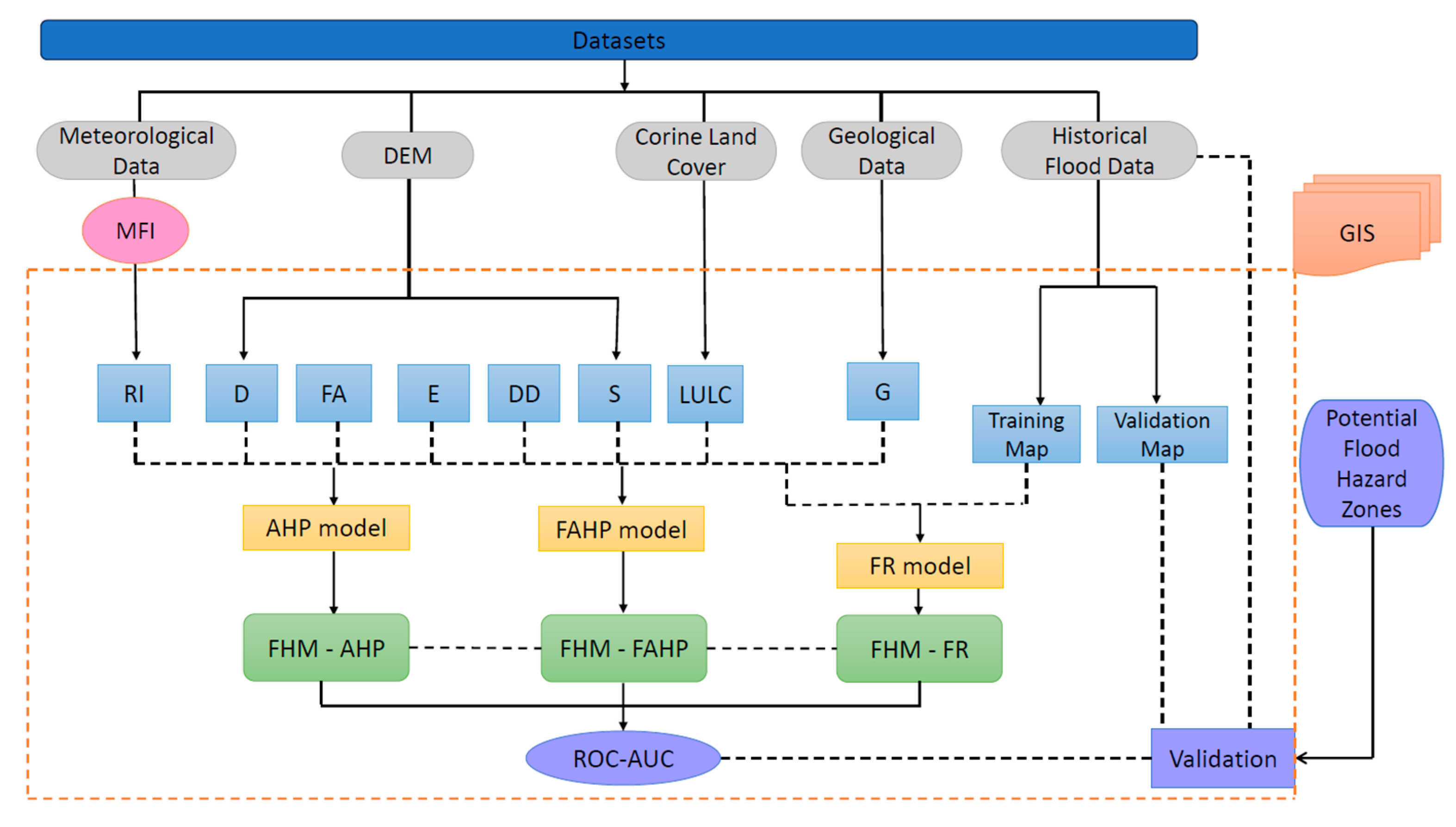
2. Materials and Methods
2.1. Study Area and Datasets
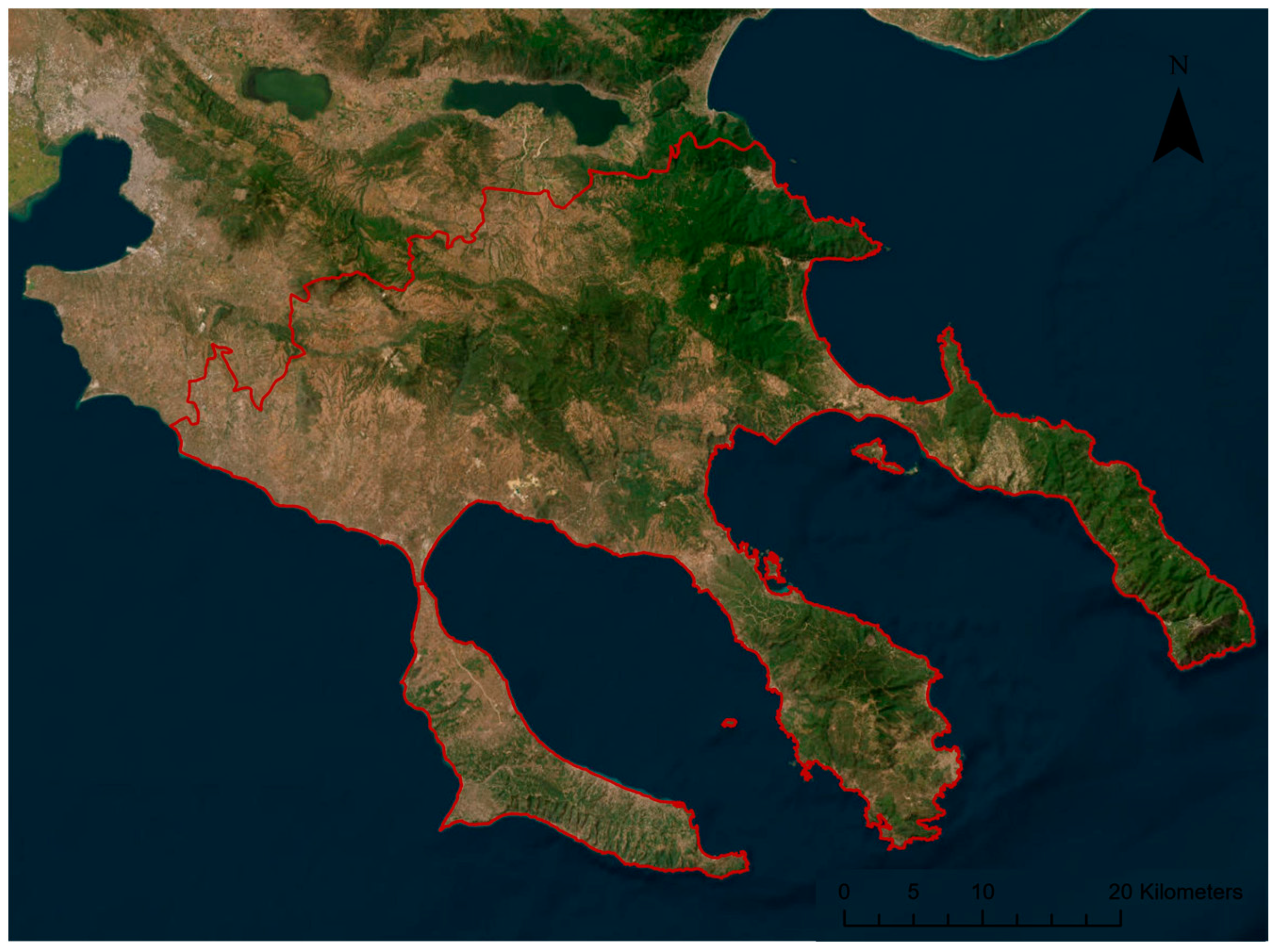
2.1.1. Study Area
2.1.2. Datasets
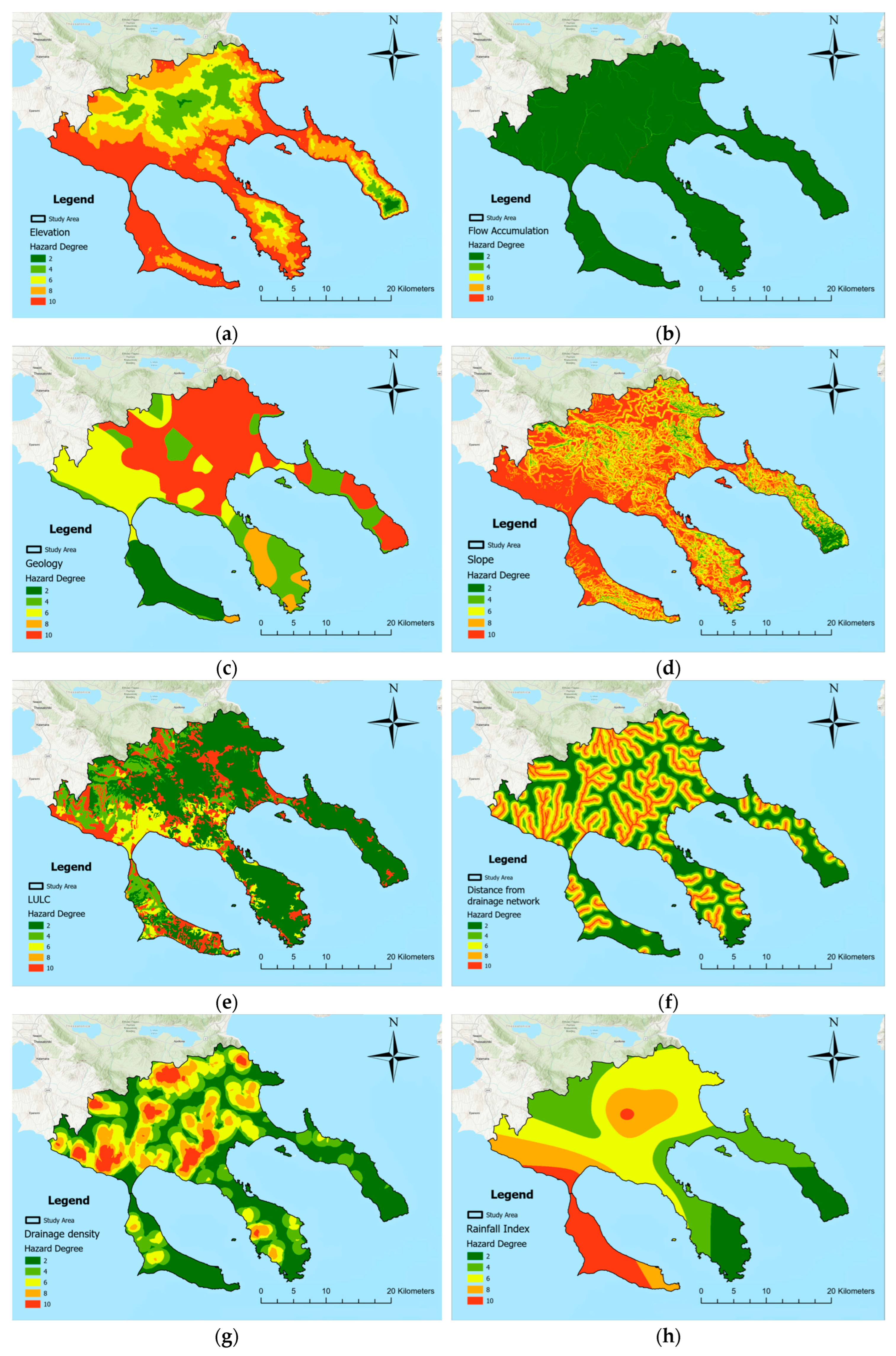
2.1.3. Flood Criteria
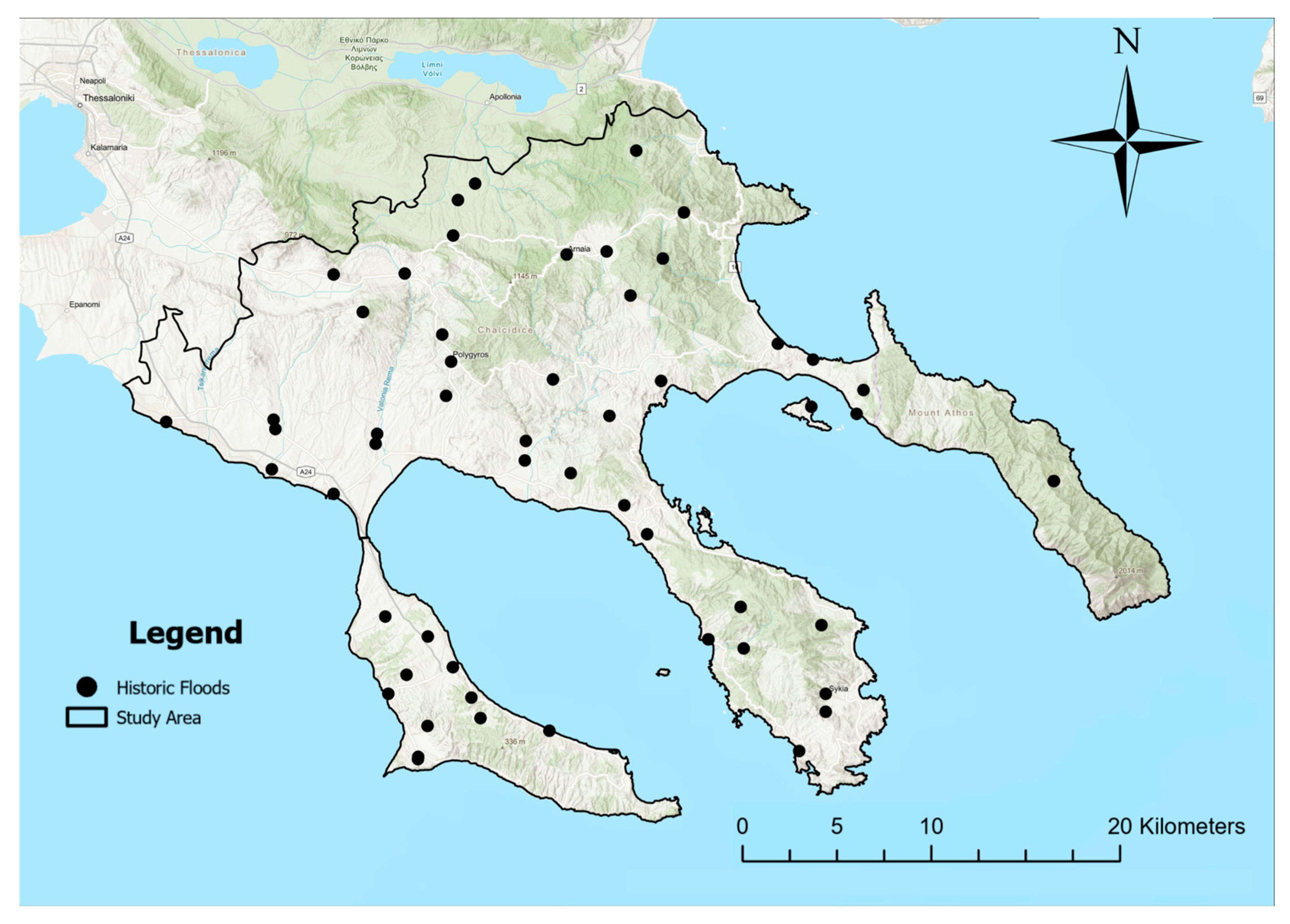
2.1.4. Flood Inventory Map
2.2. AHP
2.3. Fuzzy Sets and FAHP
2.4. Frequency Ratio (FR)
3. Results
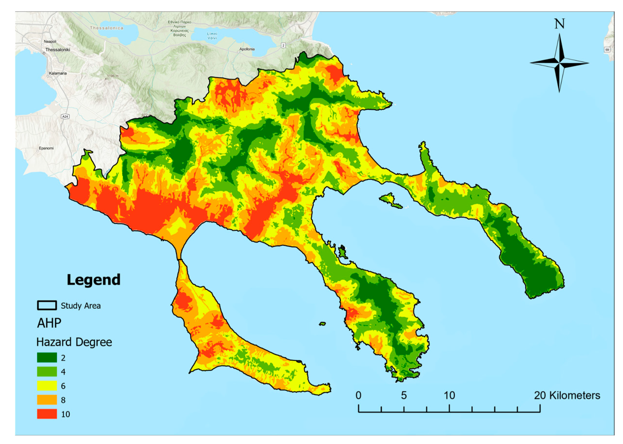
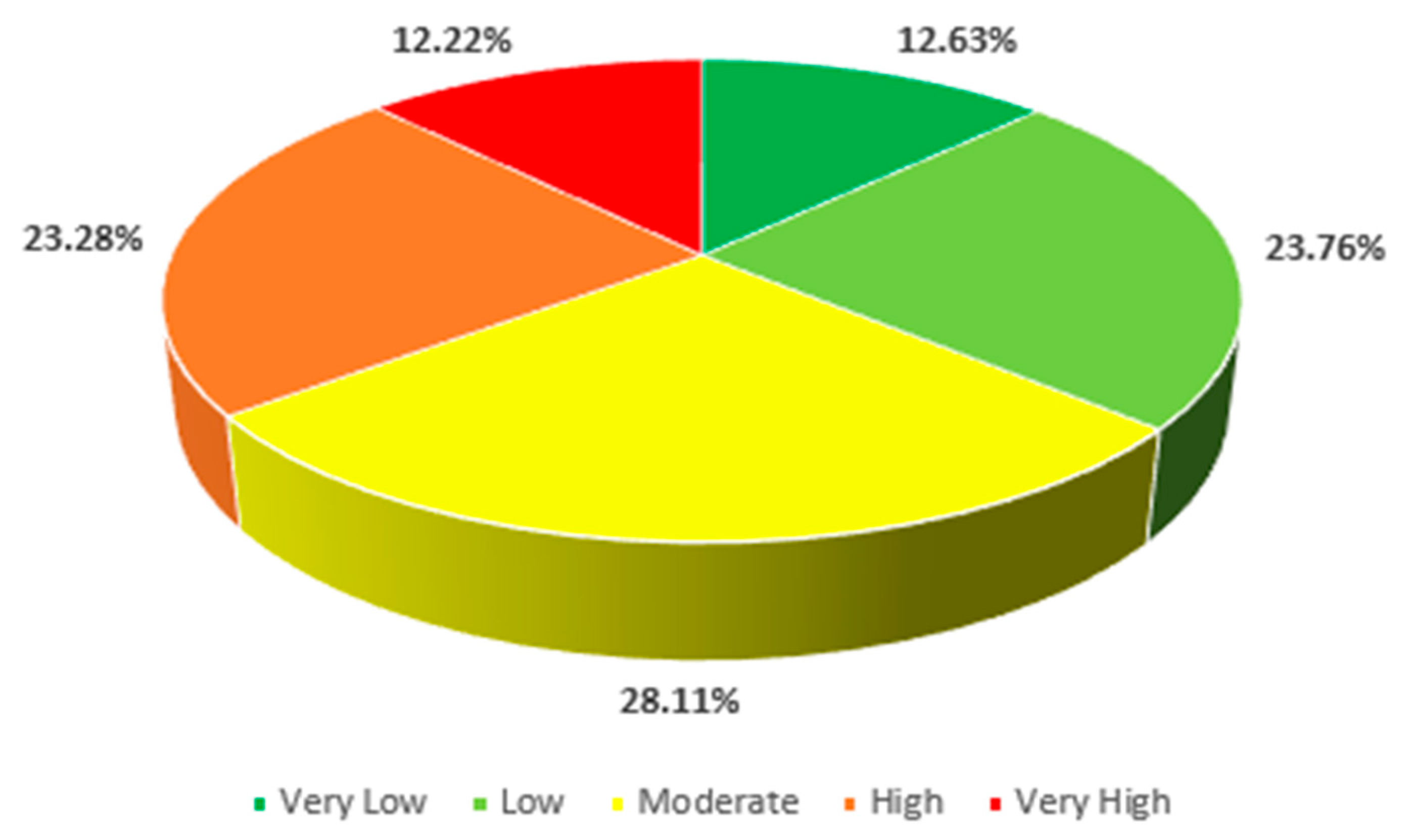
3.1. AHP Outcomes
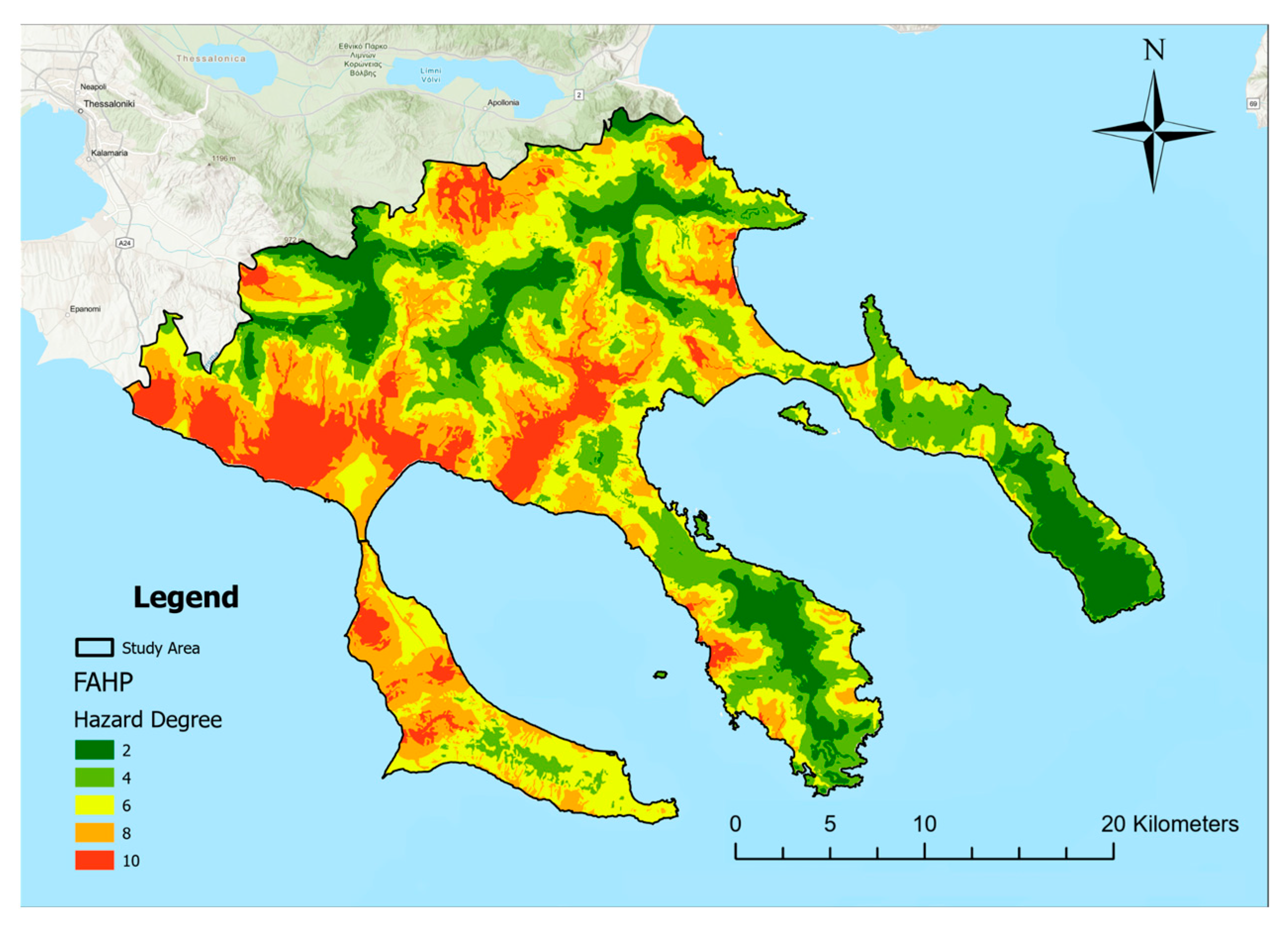
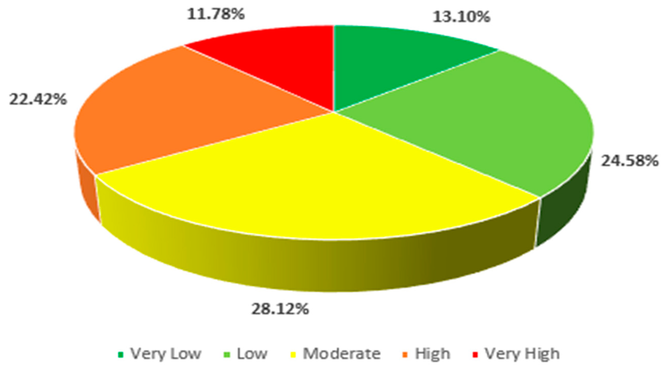
3.2. FAHP Outcomes
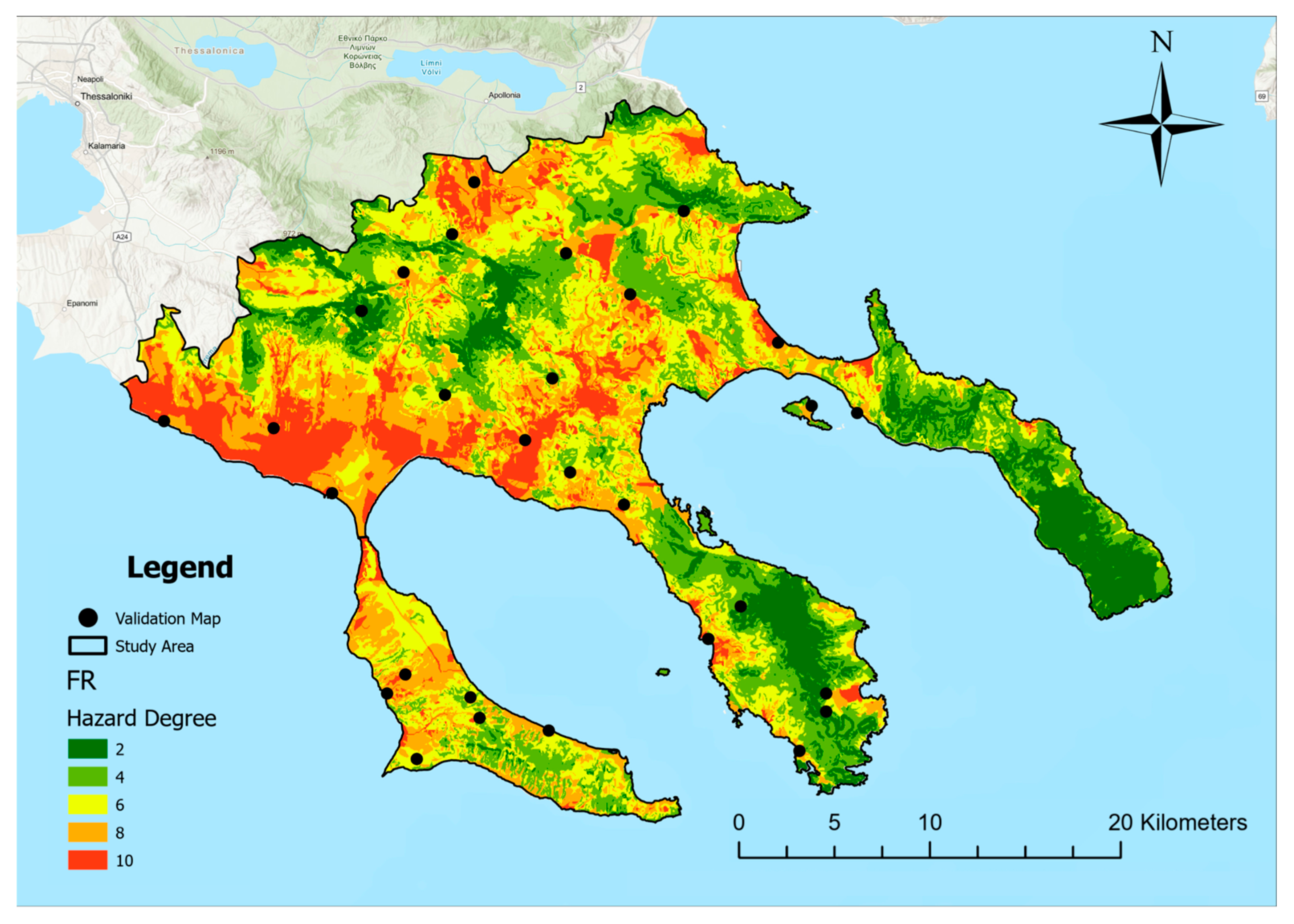
3.3. FR Model Outcomes
3.4. Validation of Flood Hazard Maps
3.4.1. FR Model Validation
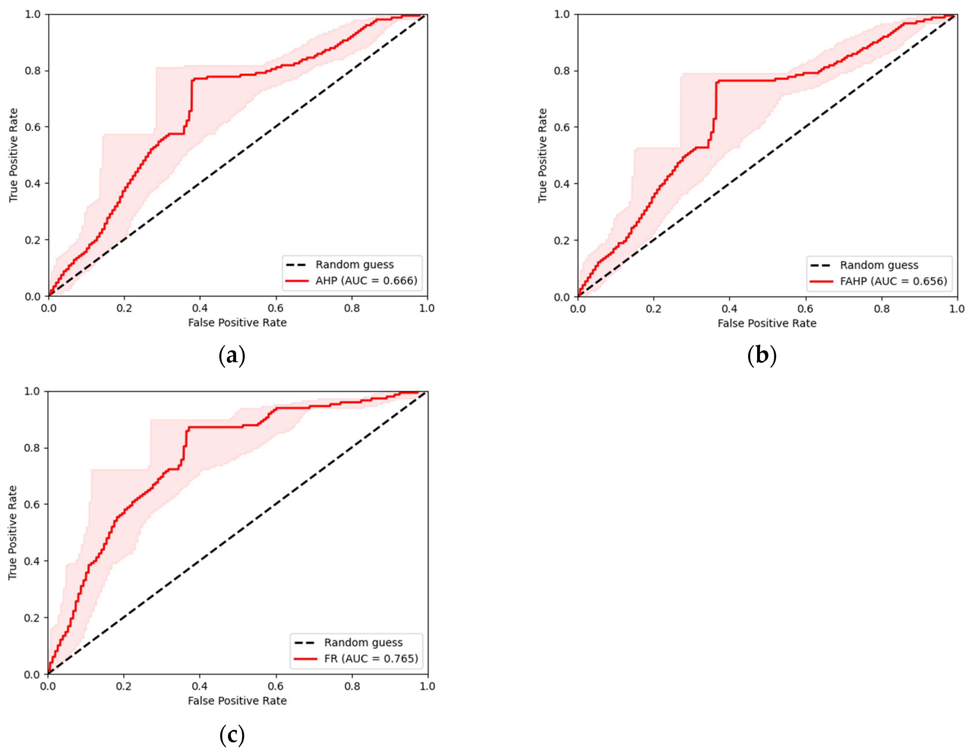
3.4.2. ROC-AUC
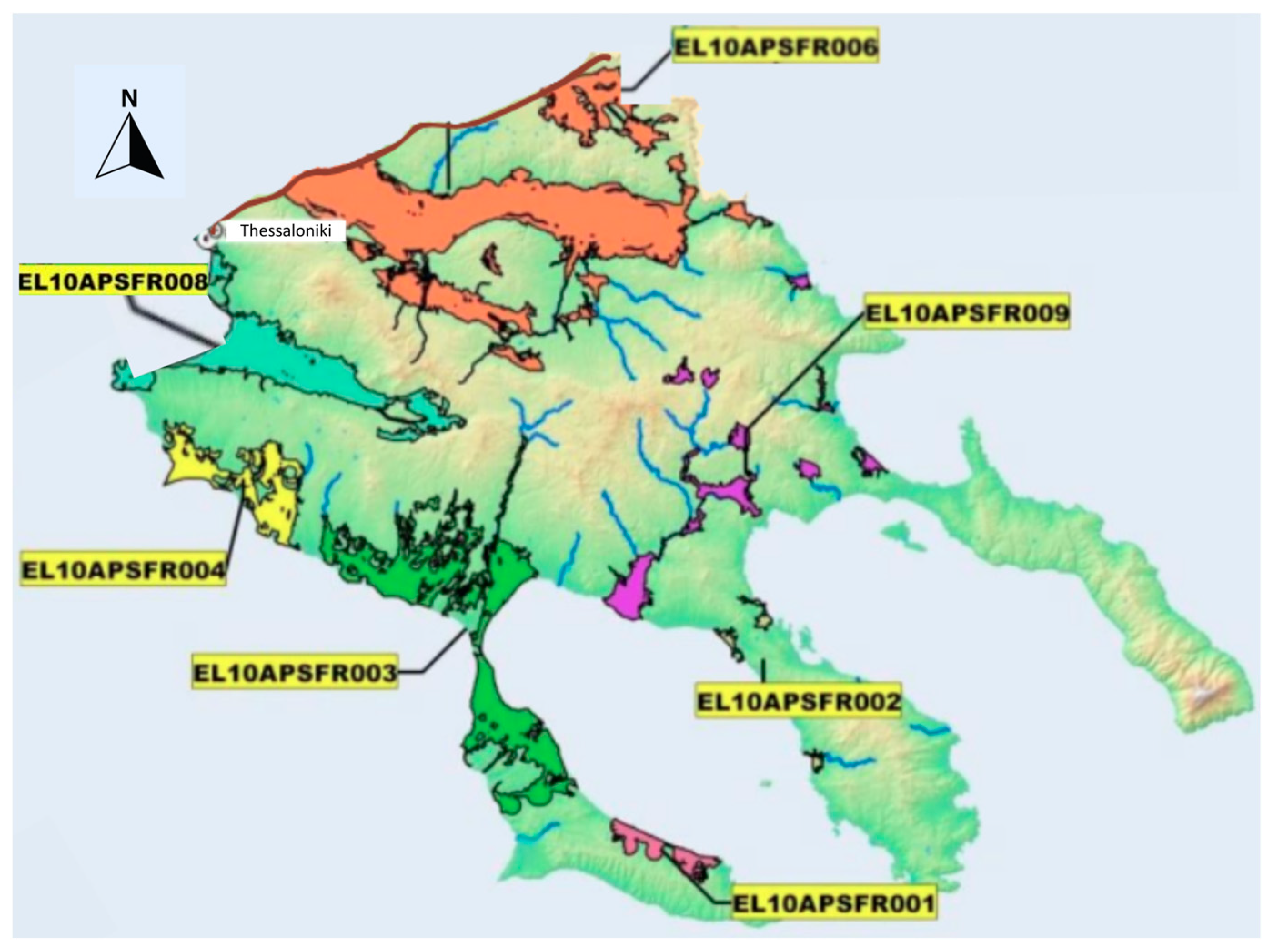
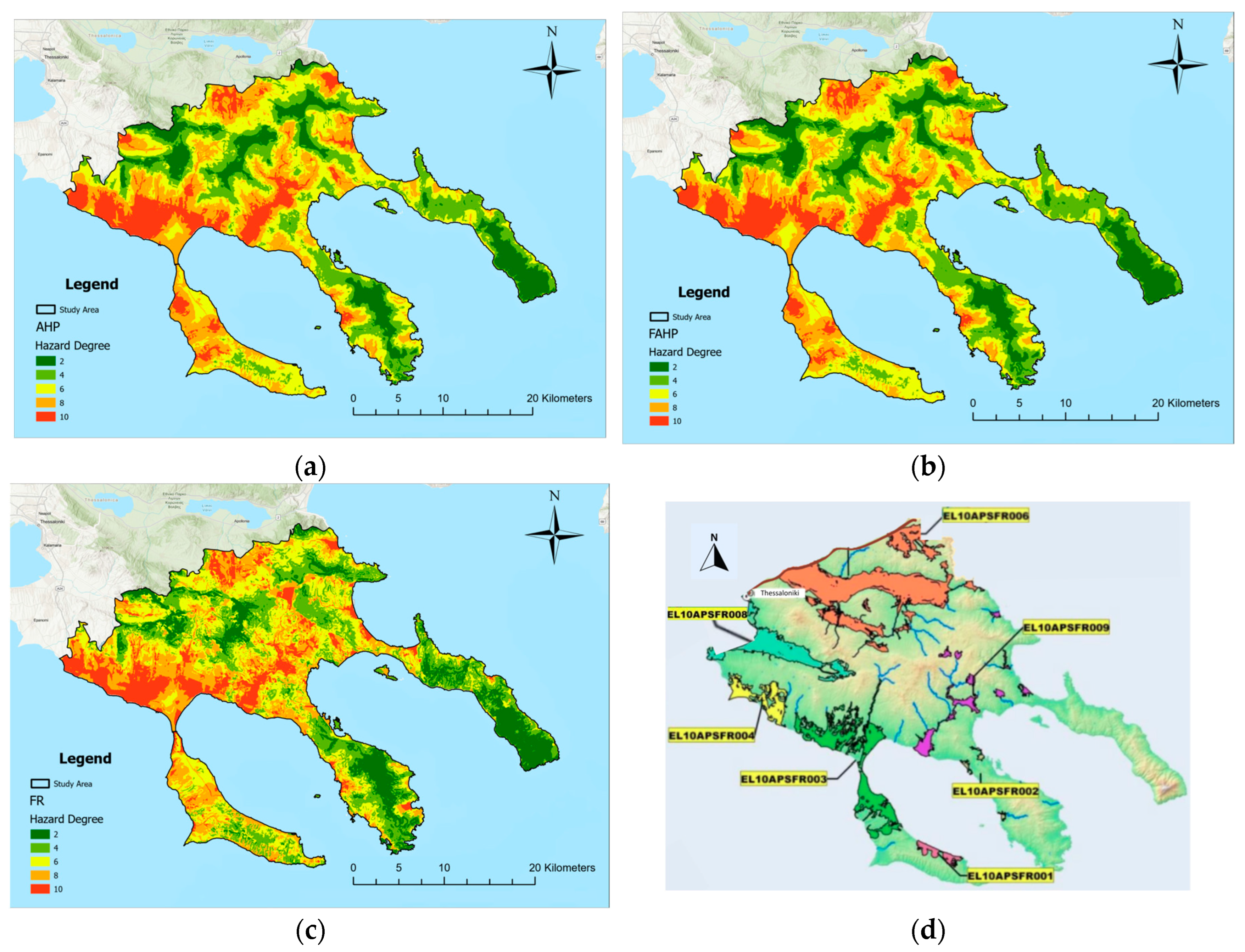
3.4.3. Comparison of the Flood Hazard Maps and the National Flood Risk Management Plans
- EL10APSFR001—The Coastal Zone of Chanioti-Polydrosso Areas of the Southern Kassandra Peninsula;
- EL10APSFR002—The Coastal Zone of Agios Nikolaos Area and other low-lying areas of Western Sithonia;
- EL10APSFR003—The Low Zone of Stream Basins of Moudania, Agios Mamas, and Northern Part of Kassandra Peninsula, Chalkidiki;
- EL10APSFR004—The Low Zone of Stream Basins of Nea Irakleia Prefecture—Kallikrateia Prefecture and Coastal zone of Epanomi;
- EL10APSFR006—Low-lying areas of the lakes Koroneia—Volvis and the Richios River watershed;
- EL10APSFR008—The Low-lying basin zone of the T66 regional ditch, the Loudias and Axios rivers, including the area of the former Lake Artzan and Gallikos, lakeshore areas of Lake Doirani, low-lying zone of the Thessaloniki urban complex, and Anthemountas stream;
- EL10APSFR009—Lowland zones of the Chavrias catchment basin and streams of the Municipality of Aristotelis.
3.4.4. Dice Similarity Coefficient (DSC)
4. Discussion
- 57% of the historical flood events occurred in areas designated as high or very high hazard by the AHP model;
- 52% of all recorded flood events took place in regions classified as high or very high hazard by the FAHP model;
- 72% of historical floods within the study area are located in zones identified as high and very high hazard by the FR model.
- According to the AHP model, 35.5% of the study area is classified as very high and high flood hazard, 36.39% as very low and low hazard, while 28.11% of the study area falls under moderate hazard.
- Based on the FAHP model, very high and high flood hazard zones cover 34.2% of the study area, very low and low hazard zones account for 37.68%, and 28.12% of the area is categorized as moderate hazard.
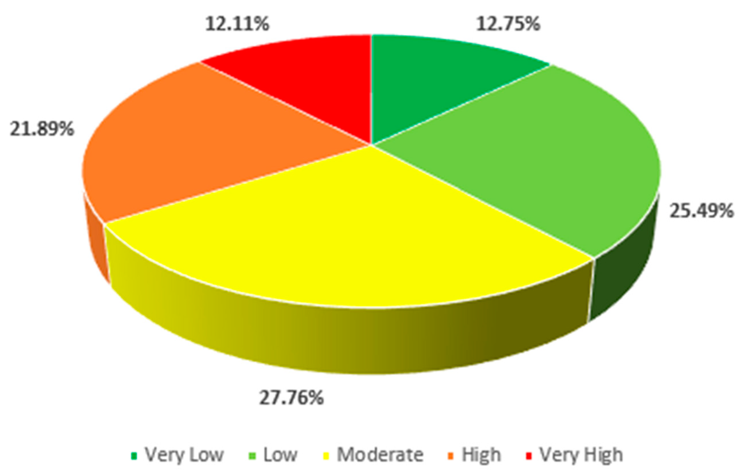
- Based upon the FR model, 34% of the study area is designated as very high and high hazard, 38.24% as low and very low hazard, and 27.76% is classified as moderate hazard.
5. Conclusions
Author Contributions
Funding
Data Availability Statement
Conflicts of Interest
Abbreviations
| GIS | Geographic Information Systems |
| MCDM | Multi-Criteria Decision Making |
| DEM | Digital Elevation Model |
| MFI | Modified Fournier Index |
| FHM | Flood Hazard Map |
| E | Elevation |
| FA | Flow Accumulation |
| DD | Drainage Density |
| RI | Rainfall Index |
| D | Distance from the drainage network |
| LULC | Land Use/Land Cover |
| G | Geology |
| S | Slope |
| AHP | Analytic Hierarchy Process |
| FAHP | Fuzzy Analytic Hierarchy Process |
| FR | Frequency Ratio |
| FL | Fuzzy Logic |
| TFN | Triangular Fuzzy Numbers |
| AUC | Area Under the Curve |
| ROC | Receiver Operating Characteristic |
References
- Weday, M.A.; Tabor, K.W.; Gemeda, D.O. Flood hazards and risk mapping using geospatial technologies in Jimma City, southwestern Ethiopia. Heliyon J. 2023, 9, e14617. [Google Scholar] [CrossRef] [PubMed]
- Zheng, Q.; Shen, S.-L.; Zhou, A.; Lyu, H.-M. Inundation risk assessment based on G-DEMATEL-AHP and its application to Zhengzhou flooding disaster. Sustain. Cities Soc. 2022, 86, 104138. [Google Scholar] [CrossRef]
- Munir, A.; Ghufran, M.A.; Ali, S.M.; Majeed, A.; Batool, A.; Khan, M.B.A.S.; Abbasi, G.H. Flood Susceptibility Assessment Using Frequency Ratio Modelling Approach in Northern Sindh and Southern Punjab, Pakistan. Pol. J. Environ. Stud. 2022, 31, 3249–3261. [Google Scholar] [CrossRef] [PubMed]
- Sarkar, D.; Saha, S.; Mondal, P. GIS-based frequency ratio and Shannon’s entropy techniques for flood vulnerability assessment in Patna district, Central Bihar, India. Int. J. Environ. Sci. Technol. 2022, 19, 8911–8932. [Google Scholar] [CrossRef]
- Cao, C.; Xu, P.; Wang, Y.; Chen, J.; Zheng, L.; Niu, C. Flash Flood Hazard Susceptibility Mapping Using Frequency Ratio and Statistical Index Methods in Coalmine Subsidence Areas. Sustainability 2016, 8, 948. [Google Scholar] [CrossRef]
- World Economic Forum. The Global Risks Report 2025. Available online: https://www.weforum.org/publications/global-risks-report-2025/ (accessed on 15 July 2025).
- Panging, A.; Koduru, S.R.; Simhachalam, A.; Baruah, L. Application of frequency ratio model for flood hazard zonation in the Dikhow River basin, Northeast India. Nat. Hazards 2025, 121, 9963–9993. [Google Scholar] [CrossRef]
- Ekmekcioğlu, Ö.; Koc, K.; Özger, M. Towards flood risk mapping based on multi-tiered decision making in a densely urbanized metropolitan city of Istanbul. Sustain. Cities Soc. 2022, 80, 103759. [Google Scholar] [CrossRef]
- Ritchie, H.; Rosado, P.; Roser, M. “Natural Disasters” Published Online at OurWorldinData.org. Available online: https://ourworldindata.org/natural-disasters (accessed on 15 July 2025).
- Tehrany, M.S.; Pradhan, B.; Jebur, M.N. Flood susceptibility analysis and its verification using a novel ensemble support vector machine and frequency ratio method. Stoch. Environ. Res. Risk Assess. 2015, 29, 1149–1165. [Google Scholar] [CrossRef]
- Pham, B.T.; Jaafari, A.; Van Phong, T.; Yen, H.P.H.; Tuyen, T.T.; Van Luong, V.; Nguyen, H.D.; Le, H.V.; Foong, L.K. GIS Based Hybrid Computational Approaches for Flash Flood Susceptibility Assessment. Geosci. Front. 2021, 12, 101105. [Google Scholar] [CrossRef]
- Rana, S.M.S.; Habib, S.M.A.; Sharifee, M.N.H.; Nasrin, S.; Rahman, S.H. Flood risk mapping of the flood-prone Rangpur division of Bangladesh using remote sensing and multi-criteria analysis. Nat. Hazards Res. 2024, 4, 20–31. [Google Scholar] [CrossRef]
- Ghorbani, M.K.; Talebbeydokhti, N.; Hamidifar, H.; Samadi, M.; Nones, M.; Rezaeitavabe, F.; Heidarifar, S. Application of Multi-Criteria Decision-Making Models for Assessment of Education Quality in Water Resources Engineering. Algorithms 2025, 18, 12. [Google Scholar] [CrossRef]
- Baalousha, H.M.; Younes, A.; Yassin, M.A.; Fahs, M. Comparison of the Fuzzy Analytic Hierarchy Process (F-AHP) and Fuzzy Logic for Flood Exposure Risk Assessment in Arid Regions. Hydrology 2023, 10, 136. [Google Scholar] [CrossRef]
- Khan, N.A.; Alzahrani, H.; Bai, S.; Hussain, M.; Tayyab, M.; Ullah, S.; Ullah, K.; Khalid, S. Flood risk assessment in the Swat river catchment through GIS-based multi-criteria decision analysis. Front. Environ. Sci. 2025, 13, 1567796. [Google Scholar] [CrossRef]
- Ibrahim, M.; Huo, A.; Ullah, W.; Ullah, S.; Xuantao, Z. An integrated approach to flood risk assessment using multi-criteria decision analysis and geographic information system. A case study from a flood-prone region of Pakistan. Front. Environ. Sci. 2025, 12, 1476761. [Google Scholar] [CrossRef]
- Hagos, Y.G.; Andualem, T.G.; Yibeltal, M.; Mengie, M.A. Flood hazard assessment and mapping using GIS integrated with multi-criteria decision analysis in upper Awash River basin, Ethiopia. Appl. Water Sci. 2022, 12, 148. [Google Scholar] [CrossRef]
- Maru, D.R.; Kumar, V.; Sharma, K.V.; Pham, Q.B.; Patel, A. Integrating GIS, MCDM, and Spatial Analysis for Comprehensive Flood Risk Assessment and Mapping in Uttarakhand, India. Geol. J. 2025; early view. [Google Scholar] [CrossRef]
- Feloni, E.; Mousadis, I.; Baltas, E. Flood vulnerability assessment using a GIS-based multi-criteria approach—The case of Attica region. J. Flood Risk Manag. 2020, 13, e12563. [Google Scholar] [CrossRef]
- Ghosh, A.; Roy, M.B.; Roy, P.K. Flood Susceptibility Mapping Using the Frequency Ratio (FR) Model in the Mahananda River Basin, West Bengal, India. In India II: Climate Change Impacts, Mitigation and Adaptation in Developing Countries; Islam, M.N., Amstel, A.V., Eds.; Springer: Cham, Switzerland, 2022; pp. 73–96. [Google Scholar] [CrossRef]
- Forson, E.D.; Amponsah, P.O.; Hagan, G.B.; Sapah, M.S. Frequency ratio-based flood vulnerability modeling over the greater Accra Region of Ghana. Model. Earth Syst. Environ. 2023, 9, 2081–2100. [Google Scholar] [CrossRef]
- Mokhtari, E.; Abdelkebir, B.; Djenaoui, A.; Hamdani, N.E.H. Integrated analytic hierarchy process and fuzzy analytic hierarchy process for Sahel watershed flood susceptibility assessment, Algeria. Water Pract. Technol. 2024, 19, 453. [Google Scholar] [CrossRef]
- Okafor, G.U.; Oriakhi, O. Flood Susceptibility Modelling Using GIS-Based Analytical Hierarchy Process (AHP) in Benin City, Nigeria. NIPES-J. Sci. Technol. Res. 2024, 6, 229–242. [Google Scholar] [CrossRef]
- Taoukidou, N.; Georgiou, P.; Karpouzos, D. Application of an A.H.P.-G.I.S. Technique for Flood Hazard Assessment in the Chalkidiki Region. Water Util. J. 2023, 32, 45–62. [Google Scholar]
- Samanta, S.; Pal, D.K.; Palsamanta, B. Flood susceptibility analysis through remote sensing, GIS and frequency ratio model. Appl. Water Sci. 2018, 8, 66. [Google Scholar] [CrossRef]
- Yaseen, Z.M. Flood hazards and susceptibility detection for Ganga river, Bihar state, India: Employment of remote sensing and statistical approaches. Results Eng. 2024, 21, 101665. [Google Scholar] [CrossRef]
- Mukhtar, M.A.; Shangguan, D.; Ding, Y.; Anjum, M.N.; Banerjee, A.; Butt, A.Q.; Yadav, N.; Li, D.; Yang, Q.; Khan, A.A.; et al. Integrated flood risk assessment in Hunza-Nagar, Pakistan: Unifying big climate data analytics and multi-criteria decision-making with GIS. Front. Environ. Sci. 2024, 12, 1337081. [Google Scholar] [CrossRef]
- Cikmaz, B.A.; Yildirim, E.; Demir, I. Flood susceptibility mapping using fuzzy analytical hierarchy process for Cedar Rapids, Iowa. Int. J. River Basin Manag. 2022, 23, 1–13. [Google Scholar] [CrossRef]
- Megahed, H.A.; Abdo, A.M.; AbdelRahman, M.A.E.; Scopa, A.; Hegazy, M.N. Frequency Ratio Model as Tools for Flood Susceptibility Mapping in Urbanized Areas: A Case Study from Egypt. Appl. Sci. 2023, 13, 9445. [Google Scholar] [CrossRef]
- Vojtek, M.; Vojteková, J.; Costache, R.; Pham, Q.B.; Lee, S.; Arshad, A.; Sahoo, S.; Linhk; Thuy, N.T.; Anh, D.T. Comparison of multi-criteria-analytical hierarchy process and machine learning-boosted tree models for regional flood susceptibility mapping: A case study from Slovakia. Geomat. Nat. Hazards Risk 2021, 12, 1153–1180. [Google Scholar] [CrossRef]
- Bedada, B.A.; Dibaba, W.T. Geoinformatics and AHP multi criteria decision making integrated flood hazard zone mapping over Modjo catchment, Awash river basin, central Ethiopia. Discov. Appl. Sci. 2025, 7, 284. [Google Scholar] [CrossRef]
- Borah, P.B.; Handique, A.; Dutta, C.K.; Bori, D.; Acharjee, S.; Longkumer, L. Assessment of flood susceptibility in Cachar district of Assam, India using GIS-based multi-criteria decision-making and analytical hierarchy process. Nat. Hazards 2025, 121, 7625–7648. [Google Scholar] [CrossRef]
- Saikia, J.; Saikia, S.; Hazarika, A. An assessment of flood susceptibility using AHP and frequency ratio (FR) in the Lakhimpur district of Assam, India. Environ. Dev. Sustain. 2024. [Google Scholar] [CrossRef]
- Malla, S.; Ohgushi, K. Flood vulnerability map of the Bagmati River basin, Nepal: A comparative approach of the analytical hierarchy process and frequency ratio model. Smart Constr. Sustain. Cities 2024, 2, 16. [Google Scholar] [CrossRef]
- Ashfaq, S.; Tufail, M.; Niaz, A.; Muhammad, S.; Alzahrani, H.; Tariq, A. Flood susceptibility assessment and mapping using GIS-based analytical hierarchy process and frequency ratio models. Glob. Planet. Chang. 2025, 251, 104831. [Google Scholar] [CrossRef]
- Mattas, C.; Karpouzos, D.; Georgiou, P.; Tsapanos, T. Two-Dimensional Modelling for Dam Break Analysis and Flood Hazard Mapping: A Case Study of Papadia Dam, Northern Greece. Water 2023, 15, 994. [Google Scholar] [CrossRef]
- Isma, F.; Kusuma, M.S.B.; Nugroho, E.O.; Adityawan, M.B. Flood hazard assessment in Kuala Langsa village, Langsa city, Aceh Province-Indonesia. Case Stud. Chem. Environ. Eng. 2024, 10, 100861. [Google Scholar] [CrossRef]
- Mandal, S.P.; Chakrabarty, A. Flash flood risk assessment for upper Teesta river basin: Using the hydrological modeling system (HEC-HMS) software. Model. Earth Syst. Environ. 2016, 2, 59. [Google Scholar] [CrossRef]
- El-Bagoury, H.; Gad, A. Integrated Hydrological Modeling for Watershed Analysis, Flood Prediction, and Mitigation Using Meteorological and Morphometric Data, SCS-CN, HEC-HMS/RAS, and QGIS. Water 2024, 16, 356. [Google Scholar] [CrossRef]
- Randa, O.T.; Krhoda, O.G.; Atela, O.J.; Akala, H. Review of flood modelling and models in developing cities and informal settlements: A case of Nairobi city. J. Hydrol. Reg. Stud. 2022, 43, 101188. [Google Scholar] [CrossRef]
- Vojtek, M.; Moradi, S.; Petroselli, A.; Vojteková, J. Comparative analysis of hydraulic and GIS-based Height Above the Nearest Drainage model for fluvial flood hazard mapping: A case of the Gidra River, Slovakia. Stoch. Environ. Res. Risk Assess. 2025, 39, 2657–2675. [Google Scholar] [CrossRef]
- Fenicia, F.; Kavetski, D.; Savenije, H.H.G.; Clark, M.P.; Schoups, G.; Pfister, L.; Freer, J. Catchment properties, function, and conceptual model representation: Is there a correspondence? Hydrol. Process. 2014, 28, 2451–2467. [Google Scholar] [CrossRef]
- Adlyansah, A.L.; Husain, S.L.; Pachri, H. Analysis of Flood Hazard Zones Using Overlay Method with Figused-Based Scoring Based on Geographic Information Systems: Case Study In Parepare City South Sulawesi Province. IOP Conf. Ser. Earth Environ. Sci. 2019, 280, 012003. [Google Scholar] [CrossRef]
- ESRI. Available online: https://doc.arcgis.com/en/sharepoint/latest/workflows/classification-methods.htm (accessed on 15 July 2025).
- ESRI. Available online: https://support.esri.com/en-us/gis-dictionary/digital-elevation-model (accessed on 15 July 2025).
- Kazakis, N.; Kougias, I.; Patsialis, T. Assessment of flood hazard areas at a regional scale using an index-based approach and Analytical Hierarchy Process: Application in Rhodope-Evros region, Greece. Sci. Total Environ. 2015, 538, 555–563. [Google Scholar] [CrossRef] [PubMed]
- Vojtek, M.; Vojteková, J. Flood Susceptibility Mapping on a National Scale in Slovakia Using the Analytical Hierarchy Process. Water 2019, 11, 364. [Google Scholar] [CrossRef]
- Ikirri, M.; Faik, F.; Echogdali, F.Z.; Antunes, I.M.H.R.; Abioui, M.; Abdelrahman, K.; Fnais, M.S.; Wanaim, A.; Id-Belqas, M.; Boutaleb, S.; et al. Flood Hazard Index Application in Arid Catchments: Case of the Taguenit Wadi Watershed, Lakhssas, Morocco. Land 2022, 11, 1178. [Google Scholar] [CrossRef]
- Ogato, G.S.; Bantider, A.; Abebe, K.; Geneletti, D. Geographic information system (GIS)-Based multicriteria analysis of flooding hazard and risk in Ambo Town and its watershed, West shoa zone, oromia regional State, Ethiopia. J. Hydrol. Reg. Stud. 2020, 27, 100659. [Google Scholar] [CrossRef]
- Wibowo, R.C.; Sarkowi, M.; Setiawan, A.F.; Yudamson, A.; Asrafil; Kurniawan, M.; Arifianto, I. Flash flood hazard areas assessment in Bandar Negeri Suoh (B.N.S.) region using an index based approaches and analytical hierarchy process. J. Phys. Conf. Ser. 2020, 1434, 012006. [Google Scholar] [CrossRef]
- Carlston, C.W. Drainage Density and Streamflow; Geological Survey Professional Paper, 422(C); U.S. Government Printing Office: Washington, DC, USA, 1963; pp. C1–C8. [CrossRef]
- Kourgialas, N.N.; Karatzas, G.P. Flood management and a GIS modelling method to assess flood-hazard areas—A case study. Hydrol. Sci. J.–J. Des. Sci. Hydrol. 2011, 56, 212–225. [Google Scholar] [CrossRef]
- Chetia, L.; Paul, S.K. Spatial Assessment of Flood Susceptibility in Assam, India: A Comparative Study of Frequency Ratio and Shannon’s Entropy Models. J. Indian Soc. Remote Sens. 2024, 52, 343–358. [Google Scholar] [CrossRef]
- Ramesh, V.; Iqbal, S.S. Urban flood susceptibility zonation mapping using evidential belief function, frequency ratio and fuzzy gamma operator models in GIS: A case study of Greater Mumbai, Maharashtra, India. Geocarto Int. 2020, 37, 581–606. [Google Scholar] [CrossRef]
- Sharma, A.; Poonia, M.; Rai, A.; Biniwale, R.B.; Tügel, F.; Holzbecher, E.; Hinkelmann, R. Flood Susceptibility Mapping Using GIS-Based Frequency Ratio and Shannon’s Entropy Index Bivariate Statistical Models: A Case Study of Chandrapur District, India. ISPRS Int. J. Geo-Inf. 2024, 13, 297. [Google Scholar] [CrossRef]
- Dey, H.; Shao, W.; Moradkhani, H.; Keim, B.D.; Peter, B.G. Urban flood susceptibility mapping using frequency ratio and multiple decision tree-based machine learning models. Nat. Hazards 2024, 120, 10365–10393. [Google Scholar] [CrossRef]
- Elsadek, W.M.; Wahba, M.; Al-Arifi, N.; Kanae, S.; El-Rawy, M. Scrutinizing the performance of GIS-based analytical Hierarchical process approach and frequency ratio model in flood prediction–Case study of Kakegawa, Japan. Ain Shams Eng. J. 2024, 15, 102453. [Google Scholar] [CrossRef]
- Tehrany, M.S.; Kumar, L.; Jebur, M.N.; Shabani, F. Evaluating the application of the statistical index method in flood susceptibility mapping and its comparison with frequency ratio and logistic regression methods. Geomat. Nat. Hazards Risk 2019, 10, 79–101. [Google Scholar] [CrossRef]
- Lahiri, N.; Contact Arjun, B.M.; Nongkynrih, J.M. Flood susceptibility mapping using Sentinel 1 and frequency ratio technique in Jinjiram River watershed, India. Environ. Monit. Assess. 2024, 196, 103. [Google Scholar] [CrossRef] [PubMed]
- Saaty, T.L. How to make a decision: The Analytic Hierarchy Process. Eur. J. Oper. Res. 1990, 48, 9–26. [Google Scholar] [CrossRef]
- Ajjur, S.B.; Mogheir, Y.K. Flood hazard mapping using a multi-criteria decision analysis and GIS (case study Gaza Governorate, Palestine). Arab. J. Geosci. 2020, 13, 44. [Google Scholar] [CrossRef]
- Saaty, T.L. A scaling method for priorities in hierarchical structures. J. Math. Psychol. 1977, 15, 234–281. [Google Scholar] [CrossRef]
- Mu, E.; Pereyra-Rojas, M. Chapter 2. Understanding the Analytic Hierarchy Process. In Practical Decision Making: An Introduction to the Analytic Hierarchy Process (AHP) Using Super Decisions; Springer: Berlin/Heidelberg, Germany, 2016; Volume 2, pp. 7–22. [Google Scholar]
- Lyu, H.M.; Zhou, W.H.; Shen, S.L.; Zhou, A.N. Inundation risk assessment of metro system using AHP and TFN-AHP in Shenzhen. Sustain. Cities Soc. 2020, 56, 102103. [Google Scholar] [CrossRef]
- Bokhari, B.F.; Tawabini, B.; Baalousha, H.M. A fuzzy analytical hierarchy process -GIS approach to flood susceptibility mapping in NEOM, Saudi Arabia. Front. Water 2024, 6, 1388003. [Google Scholar] [CrossRef]
- Yang, X.; Ding, J.; Hou, H. Application of a triangular fuzzy AHP approach for flood risk evaluation and response measures analysis. Nat. Hazards 2013, 68, 657–674. [Google Scholar] [CrossRef]
- Meshram, S.G.; Alvandi, E.; Singh, V.P.; Meshram, C. Comparison of AHP and fuzzy AHP models for prioritization of watersheds. Soft Comput. 2019, 23, 13615–13625. [Google Scholar] [CrossRef]
- Van Laarhoven, P.J.M.; Pedrycz, W. A fuzzy extension of Saaty’s priority theory. Fuzzy Sets Syst. 1983, 11, 229–241. [Google Scholar] [CrossRef]
- Chang, D.-Y. Applications of the extent analysis method on fuzzy AHP. Eur. J. Oper. Res. 1996, 95, 649–655. [Google Scholar] [CrossRef]
- Buckley, J.J. Fuzzy Hierarchical Analysis. Fuzzy Sets Syst. 1985, 17, 233–247. [Google Scholar] [CrossRef]
- Boender, C.G.E.; Graan, J.G.; Lootsma, F.A. Multi-criteria decision analysis with fuzzy pairwise comparisons. Fuzzy Sets Syst. 1989, 29, 133–143. [Google Scholar] [CrossRef]
- Senan, C.P.C.; Ajin, R.S.; Danumah, J.H.; Costache, R.; Arabameri, A.; Rajaneesh, A.; Sajinkumar, K.S.; Kuriakose, S.L. Flood vulnerability of a few areas in the foothills of the Western Ghats: A comparison of AHP and F-AHP models. Stoch. Environ. Res. Risk Assess. 2023, 37, 527–556. [Google Scholar] [CrossRef] [PubMed]
- Jovčić, S.; Průša, S.; Samson, J.; Lazarević, D. A fuzzy-AHP approach to evaluate the criteria of third-party logistics (3PL) service provider. Int. J. Traffic Transp. Eng. 2019, 9, 280–289. [Google Scholar] [CrossRef]
- Murty, R.L.N.; Kondamudi, S.G.; Suryanarayana, M.V.; Giribabu, P. Application of Buckley’s Fuzzy AHP to identify the most Important Factor Affecting the Unorganized Micro-Entrepreneurs’ Borrowing Decision. Int. J. Manag. 2020, 11, 665–674. [Google Scholar] [CrossRef]
- Zadeh, L.A. Fuzzy Sets. Inf. Control 1965, 8, 338–353. [Google Scholar] [CrossRef]
- Zhou, X. Fuzzy analytical network process implementation with matlab. In MATLAB-A Fundamental Tool for Scientific Computing and Engineering Applications; InTech: Rijeka, Croatia, 2012; Volume 3. [Google Scholar] [CrossRef]
- Rahmati, O.; Pourghasemi, H.R.; Zeinivand, H. Flood Susceptibility Mapping Using Frequency Ratio and Weights-of-Evidence Models in the Golastan Province, Iran. Geocarto Int. 2016, 31, 42–70. [Google Scholar] [CrossRef]
- Majeed, M.; Lu, L.; Anwar, M.M.; Tariq, A.; Qin, S.; El-Hefnawy, M.E.; El-Sharnouby, M.; Li, Q.; Alasmari, A. Prediction of flash flood susceptibility using integrating analytic hierarchy process (AHP) and frequency ratio (FR) algorithms. Front. Environ. Sci. 2023, 10, 1037547. [Google Scholar] [CrossRef]
- Sarkar, D.; Modal, P. Flood vulnerability mapping using frequency ratio (FR) model: A case study on Kulik river basin, Indo-Bangladesh Barind region. Appl. Water Sci. 2020, 10, 17. [Google Scholar] [CrossRef]
- Lee, M.J.; Kang, J.; Jeon, S. Application of frequency ratio model and validation for predictive flooded area susceptibility mapping using GIS. In Proceedings of the 2012 IEEE International Geoscience and Remote Sensing Symposium, Munich, Germany, 22–27 July 2012; IEEE: Piscataway, NJ, USA, 2012; pp. 895–898. [Google Scholar] [CrossRef]
- Tehrany, M.S.; Pradhan, B.; Jebur, M.N. Spatial prediction of flood susceptible areas using rule based decision tree (DT) and a novel ensemble bivariate and multivariate statistical models in GIS. J. Hydrol. 2013, 504, 69–79. [Google Scholar] [CrossRef]
- Abdo, H.G.; Zeng, T.; Alshayeb, M.J.; Prasad, P.; Mohamed Ahmed, M.F.; Albanai, J.A.; Alharbi, M.M.; Mallick, J. Multi-criteria analysis and geospatial applications-based mapping flood vulnerable areas: A case study from the eastern Mediterranean. Nat. Hazards 2025, 121, 1003–1031. [Google Scholar] [CrossRef]
- Varma, A.K.; Dhote, A.; Mathew, A.; Naresh, C.; Shekar, P.R. Flood hazard zonation using remote sensing, geographic information system, and analytic hierarchy process in the Bhagirathi River Basin, Uttarakhand, India. Results Earth Sci. 2025, 3, 100105. [Google Scholar] [CrossRef]
- Ali, Z.; Dahri, N.; Vanclooster, M.; Mehmandoostkotlar, A.; Labbaci, A.; Ben Zaied, M.; Ouessar, M. Hybrid Fuzzy AHP and Frequency Ratio Methods for Assessing Flood Susceptibility in Bayech Basin, Southwestern Tunisia. Sustainability 2023, 15, 15422. [Google Scholar] [CrossRef]
- Xue, F.; Guo, L.; Bialkowski, A.; Abbosh, A.M. Integrated Boundary-Overlap-Size Metric for Local Assessment of Deep Learning Methods in Medical Microwave Imaging. IEEE J. Electromagn. RF Microw. Med. Biol. 2025, 9, 229–239. [Google Scholar] [CrossRef]
- Anand, A.; Imasu, R.; Dhaka, S.K.; Patra, P.K. Domain Adaptation and Fine-Tuning of a Deep Learning Segmentation Model of Small Agricultural Burn Area Detection Using High-Resolution Sentinel-2 Observations: A Case Study of Punjab, India. Remote Sens. 2025, 17, 974. [Google Scholar] [CrossRef]


| Data | Source | Spatial Resolution | Description |
|---|---|---|---|
| DEM | Hellenic Military Geographical Service | 80 × 80 | Processed in GIS Pro 3.4.3 |
| Rainfall | Gauge stations in the area | Processed first in Excel and then in GIS Pro 3.4.3 | |
| LULC | CORINE Land Cover 2018, EEA (European Environment Agency) | 80 × 80 | Processed in GIS Pro 3.4.3 |
| Geological data | Hellenic Survey of Geology & Mineral Exploration (H.S.G.M.E.) | 80 × 80 | Processed in GIS Pro 3.4.3 |
| Historical Flood Data | Hellenic Ministry of Environment and Energy, the online database of the National Observatory of Athens (meteo.gr), and other published reports | 80 × 80 | Processed first in Excel and then in GIS Pro 3.4.3 to create training and validation maps |
| Elevation (m) | Hazard Degree |
|---|---|
| 943–1918 | 2 |
| 568–943 | 4 |
| 351–568 | 6 |
| 163–351 | 8 |
| 6–163 | 10 |
| Flow Accumulation (m) | Hazard Degree |
|---|---|
| 0–1.173 | 2 |
| 1.173–4.589 | 4 |
| 4.589–11.962 | 6 |
| 11.962–30.535 | 8 |
| 30.535–65.229 | 10 |
| Geology Categories | Hazard Degree |
|---|---|
| Alluvial | 2 |
| Quaternary deposits | 4 |
| Neogene sediments | 6 |
| Carbonate rocks | 8 |
| Crystalline rocks | 10 |
| Slope (%) | Hazard Degree |
|---|---|
| 47.2–126.8 | 2 |
| 26.9–47.2 | 4 |
| 15.4–26.9 | 6 |
| 6.4–15.4 | 8 |
| 0–6.4 | 10 |
| LULC Categories | Hazard Degree | Distribution, % |
|---|---|---|
| Forests, Transitional woodland-shrublands, Sclerophyllous vegetation | 2 | 57.07 |
| Non-irrigated-arable land | 4 | 13.17 |
| Vineyards, Olive groves, Natural pastures | 6 | 10.10 |
| Meadows, Sports, and recreation facilities | 8 | 0.89 |
| Coastal marshes, Water bodies, Industrial or commercial zones, Urban development, Mines | 10 | 18.77 |
| Distance from Drainage Network (m) | Hazard Degree |
|---|---|
| >2000 | 2 |
| 1000–2000 | 4 |
| 500–1000 | 6 |
| 200–500 | 8 |
| <200 | 10 |
| Drainage Density (km/km2) | Hazard Degree |
|---|---|
| 0–0.073 | 2 |
| 0.073–0.189 | 4 |
| 0.189–0.313 | 6 |
| 0.313–0.472 | 8 |
| 0.472–0.776 | 10 |
| Rainfall Index | Hazard Degree |
|---|---|
| 15.62–34.85 | 2 |
| 34.85–46.43 | 4 |
| 46.43–56.18 | 6 |
| 56.18–68.03 | 8 |
| 68.03–82.78 | 10 |
| Definition | Numeric Value |
|---|---|
| Extremely important | 9 |
| 8 | |
| Very strongly more important | 7 |
| 6 | |
| Strongly more important | 5 |
| 4 | |
| Moderately more important | 3 |
| 2 | |
| Equally important | 1 |
| n | RI |
|---|---|
| 1 | 0.00 |
| 2 | 0.00 |
| 3 | 0.58 |
| 4 | 0.90 |
| 5 | 1.12 |
| 6 | 1.24 |
| 7 | 1.32 |
| 8 | 1.41 |
| 9 | 1.45 |
| Definition | Numeric Value | Triangular Fuzzy Number | Fuzzy Reciprocal |
|---|---|---|---|
| Extremely important | 9 | (9,9,9) | (1/9,1/9,1/9) |
| Intermediate value | 8 | (7,8,9) | (1/9,1/8,1/7) |
| Very strongly more important | 7 | (6,7,8) | (1/8,1/7,1/6) |
| Intermediate value | 6 | (5,6,7) | (1/7,1/6,1/5) |
| Strongly more important | 5 | (4,5,6) | (1/6,1/5,1/4) |
| Intermediate value | 4 | (3,4,5) | (1/5,1/4,1/3) |
| Moderately more important | 3 | (2,3,4) | (1/4,1/3,1/2) |
| Intermediate value | 2 | (1,2,3) | (1/3,1/2,1) |
| Equally important | 1 | (1,1,1) | (1,1,1) |
| E | FA | DD | RI | D | LULC | G | S | |
|---|---|---|---|---|---|---|---|---|
| E | 1 | 1 | 2 | 3 | 4 | 4 | 5 | 7 |
| FA | 1 | 1 | 2 | 3 | 4 | 4 | 5 | 7 |
| DD | 1/2 | 1/2 | 1 | 2 | 3 | 4 | 5 | 6 |
| RI | 1/3 | 1/3 | 1/2 | 1 | 2 | 3 | 4 | 6 |
| D | 1/4 | 1/4 | 1/3 | 1/2 | 1 | 2 | 3 | 5 |
| LULC | 1/4 | 1/4 | 1/4 | 1/3 | 1/2 | 1 | 2 | 3 |
| G | 1/5 | 1/5 | 1/5 | 1/4 | 1/3 | 1/2 | 1 | 2 |
| S | 1/7 | 1/7 | 1/6 | 1/6 | 1/5 | 1/3 | 1/2 | 1 |
| Flood Hazard Degree | Area, km2 | Flood Hazard |
|---|---|---|
| 2 | 402.20 | Very Low |
| 4 | 756.45 | Low |
| 6 | 894.84 | Moderate |
| 8 | 741.11 | High |
| 10 | 389.03 | Very High |
| E | FA | DD | RI | D | LULC | G | S | |
|---|---|---|---|---|---|---|---|---|
| E | (1,1,1) | (1,1,1) | (1,2,3) | (2,3,4) | (3,4,5) | (3,4,5) | (4,5,6) | (6,7,8) |
| FA | (1,1,1) | (1,1,1) | (1,2,3) | (2,3,4) | (3,4,5) | (3,4,5) | (4,5,6) | (6,7,8) |
| DD | (1/3,1/2,1) | (1/3,1/2,1) | (1,1,1) | (1,2,3) | (2,3,4) | (3,4,5) | (4,5,6) | (5,6,7) |
| RI | (1/4,1/3,1/2) | (1/4,1/3,1/2) | (1/3,1/2,1) | (1,1,1) | (1,2,3) | (2,3,4) | (3,4,5) | (5,6,7) |
| D | (1/5,1/4,1/3) | (1/5,1/4,1/3) | (1/4,1/3,1/2) | (1/3,1/2,1) | (1,1,1) | (1,2,3) | (2,3,4) | (4,5,6) |
| LULC | (1/5,1/4,1/3) | (1/5,1/4,1/3) | (1/5,1/4,1/3) | (1/4,1/3,1/2) | (1/3,1/2,1) | (1,1,1) | (1,2,3) | (2,3,4) |
| G | (1/6,1/5,1/4) | (1/6,1/5,1/4) | (1/6,1/5,1/4) | (1/5,1/4,1/3) | (1/4,1/3,1/2) | (1/3,1/2,1) | (1,1,1) | (1,2,3) |
| S | (1/8,1/7,1/6) | (1/8,1/7,1/6) | (1/7,1/6,1/5) | (1/7,1/6,1/5) | (1/6,1/5,1/4) | (1/4,1/3,1/2) | (1/3,1/2,1) | (1,1,1) |
| Flood Hazard Degree | Area, km2 | Flood Hazard |
|---|---|---|
| 2 | 417.05 | Very Low |
| 4 | 782.62 | Low |
| 6 | 895.24 | Moderate |
| 8 | 713.72 | High |
| 10 | 374.99 | Very High |
| Flood Hazard Degree | Area, km2 | Flood Hazard |
|---|---|---|
| 2 | 405.79 | Very Low |
| 4 | 811.63 | Low |
| 6 | 883.76 | Moderate |
| 8 | 696.97 | High |
| 10 | 385.47 | Very High |
| Map Pair | DSC |
|---|---|
| AHP VS FAHP | 0.981 |
| AHP VS FR | 0.814 |
| FAHP VS FR | 0.807 |
Disclaimer/Publisher’s Note: The statements, opinions and data contained in all publications are solely those of the individual author(s) and contributor(s) and not of MDPI and/or the editor(s). MDPI and/or the editor(s) disclaim responsibility for any injury to people or property resulting from any ideas, methods, instructions or products referred to in the content. |
© 2025 by the authors. Licensee MDPI, Basel, Switzerland. This article is an open access article distributed under the terms and conditions of the Creative Commons Attribution (CC BY) license (https://creativecommons.org/licenses/by/4.0/).
Share and Cite
Taoukidou, N.; Karpouzos, D.; Georgiou, P. Flood Hazard Assessment Through AHP, Fuzzy AHP, and Frequency Ratio Methods: A Comparative Analysis. Water 2025, 17, 2155. https://doi.org/10.3390/w17142155
Taoukidou N, Karpouzos D, Georgiou P. Flood Hazard Assessment Through AHP, Fuzzy AHP, and Frequency Ratio Methods: A Comparative Analysis. Water. 2025; 17(14):2155. https://doi.org/10.3390/w17142155
Chicago/Turabian StyleTaoukidou, Nikoleta, Dimitrios Karpouzos, and Pantazis Georgiou. 2025. "Flood Hazard Assessment Through AHP, Fuzzy AHP, and Frequency Ratio Methods: A Comparative Analysis" Water 17, no. 14: 2155. https://doi.org/10.3390/w17142155
APA StyleTaoukidou, N., Karpouzos, D., & Georgiou, P. (2025). Flood Hazard Assessment Through AHP, Fuzzy AHP, and Frequency Ratio Methods: A Comparative Analysis. Water, 17(14), 2155. https://doi.org/10.3390/w17142155