Numerical Study of Turbulent Open-Channel Flow Through Submerged Rigid Vegetation

Abstract

In the present study, three-dimensional turbulent, subcritical open-channel flow (Fr = 0.19) through submerged rigid vegetation is numerically investigated using the ANSYS FLUENT solver (v. 22. 1). The Volume of Fluid (VOF) method is applied for free-surface tracking, while the standard k-ε turbulence model is employed for turbulence closure. Vegetation is modeled as vertical rigid cylinders fixed at the bottom of the channel. Regarding the arrangement of the stems, two cases are examined. In the first case, a linear arrangement of three equally spaced vegetative stems is located transversely at the center of the channel, while in the second case, a parallel arrangement of fifteen equidistant vegetative stems is located downstream of the channel center. In both cases, the vertical velocity profile within the submerged vegetation layer deviates significantly from that of the upper non-vegetated layer, which generally adheres to the logarithmic velocity distribution. In the second case, flow field repeatability is observed after the third stem series, particularly in terms of velocity profiles. Additionally, the structure of turbulence is noticeably affected in the vicinity of the stems, resulting in higher eddy viscosity values near each stem’s crest area. Furthermore, a localized drop in the free surface is recorded above the vegetated region, while a slight rise is observed upstream of each stem series, consistent with subcritical open-channel flow.

1. Introduction

Vegetation plays a vital role in modifying flow characteristics in both natural and artificial open channels, as well as in riverine systems. Historically, the presence of vegetation in rivers has often been considered undesirable because it increases flow resistance by acting as an obstruction and reduces flow velocity, as well as channel’s flood conveyance and floodplain discharge capacity [1,2]. However, recent research has focused on the benefits of vegetation, such as improving water quality by acting as a natural filter that removes pollutants and produces oxygen [1,3,4]. In addition, vegetation contributes to habitat diversity through the modification of the velocity field and thus supports the diversity of aquatic wildlife. Furthermore, it protects riverbanks from erosion and ensures their stability by reducing flow velocity and increasing sediment deposition, making vegetation a valuable tool for maintaining the morphological characteristics of rivers [3,4,5]. Therefore, gaining a thorough understanding of the interactions between vegetation and flow field is deemed crucial to the ecological management and rehabilitation of rivers [3].

In general, the vegetation in a river system is divided into riparian and aquatic vegetation, according to its position in the open channel. Riparian vegetation is found in the riparian zone of a river and grows along the riverbanks, extending to the floodplain boundary [6]. On the other hand, aquatic vegetation (or macrophytes) usually grows in the river bed and can be further subdivided into submerged, emergent, and floating, depending on the vegetation–flow depth relationship [3]. It can also be classified into flexible (herbaceous) and rigid (typically woody or arborescent) depending on its potential to be deformed by the flow [7]. Submerged vegetation includes those macrophytes that have a root system and are entirely beneath the water surface. Emergent vegetation [8] includes macrophytes whose root system is beneath the water surface, but most of the stem and leaves are above the water. The macrophytes of floating vegetation, on the other hand, may float freely on the water surface or have roots at the bottom and floating leaves at the surface [6]. Among these categories, submerged vegetation exerts the most profound influence on flow structure [9].

The presence of submerged vegetation in open-channel flows has a direct effect on the flow field, due to the highly complex interactions between vegetation and the flow. In particular, submerged vegetation causes an increase in flow resistance, resulting in a decrease in flow velocity within the vegetated area compared with the area above, where the effect of vegetation is negligible and the velocity profile follows the logarithmic law [10]. Moreover, the damping of turbulence is observed within the vegetated area [1].

In the area between the crest of the vegetated zone and the free surface, a shear layer develops in the form of coherent vortices due to Kelvin–Helmholtz instability, which is responsible for transport phenomena in the transverse direction of the flow. It is essential to recognize that the shear layer is generated when the momentum absorption is strong at the interface due to the presence of the vegetation. This produces an inflection point in the velocity profile close to the vegetation height, which is necessary for Kelvin–Helmholtz instability to appear [1].

This paper focuses on the effect of submerged rigid vegetation on flow characteristics, including velocity and turbulence intensity distributions, as well as free-surface formation. To this end, numerical simulations of three-dimensional open-channel flow are conducted with various stem arrangements fixed at the bottom of the channel. Furthermore, the repeatability of the flow structure is examined for the case of the parallel arrangement of stem series. For the numerical simulations presented herein, the ANSYS FLUENT code [11] was applied. The numerically predicted results are juxtaposed with the corresponding velocity and eddy viscosity distributions for the case of the flat bottom (without the presence of stems). Based on the subsequent simulations, the effect of rigid stems on the flow characteristics is quantitatively studied in terms of both velocity and turbulent eddy viscosity values. Ultimately, the main goal of this study is to delve deeper into how submerged rigid vegetation affects hydrodynamics in open-channel flows, which remains a crucial factor considered for the ecological management and restoration of aquatic ecosystems.

2. Formulation

For the numerical simulation of steady, turbulent, subcritical open-channel flow, the three-dimensional (3D) RANS equations were applied. For turbulence closure, the standard k-ε two-equation turbulence model [12] was used, implementing the standard values of its constants.

The free-surface elevation was tracked using a modified version of the Volume of Fluid (VOF) method developed by Hirt and Nichols [13]. This approach is suitable for multiphase flows involving immiscible fluids. In open-channel flow, the governing equations at the water–air interface are conveyed in a single-fluid form. The physical properties of this fluid are determined by averaging the corresponding properties of air and water based on their volume fractions. For instance, the local fluid density is expressed as

$$\rho =F{\rho }_{water}+\left(1-F\right){\rho }_{air},$$

(1)

where F represents the variable for the water volume fraction.

The transport of the volume fraction F is governed by the following continuity equation:

$${\displaystyle \frac{\partial F}{\partial t}}+u_i{\displaystyle \frac{\partial F}{{\partial x}_i}}=0.$$

(2)

In the numerical implementation of VOF using a finite volume method, F is defined in each computational cell as

$$F={\displaystyle \frac{{\delta V}_{water}}{\delta V_{cell}}}$$

(3)

where δV_cell represents the volume of the computational cell and δV_water represents the fraction of the volume of water in the cell. Therefore, F = 1, F = 0, or 0 < F < 1, indicating that the cell is full of water, is full of air, or contains the water–air interface, respectively. Herein, the water free surface was identified when F was set to 0.5.

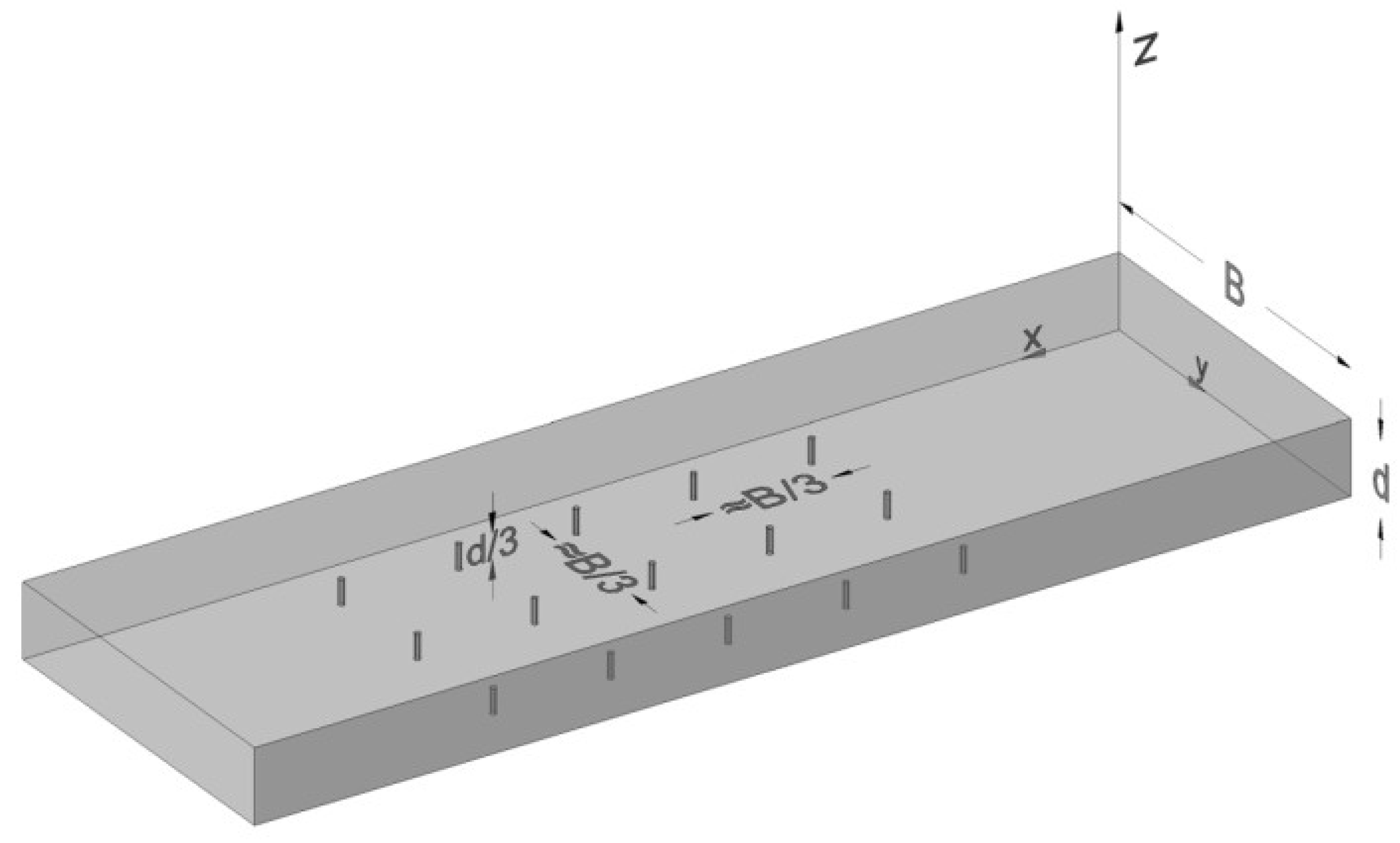
3. Computational Setup

Turbulent open-channel flow through submerged rigid vegetation in different arrangements was considered. The channel geometry and upstream flow conditions are selected to align with prior experimental setups established by Rajaratnam and Nwachukwu [14] and simulated by Koutrouveli et al. [15]. Specifically, the rectangular channel was 36.576 m long and 0.9144 m wide, with bottom slope S₀ = 10⁻⁴. The flow was considered to be subcritical, with Froude number Fr = 0.19, normal depth d = 0.189 m, and bulk mean velocity U₀ = 0.262 m/s. The corresponding Reynolds number based on the hydraulic radius was Re = 1.4 × 10⁵ or Re = 3.9 × 10³ based on the diameter, D, of the vegetated stem, for water density ρ = 998.2 kg/m³ and kinematic viscosity ν = 1.005 × 10⁻⁶ m²/s. The channel bed and side walls were assumed to be hydraulically smooth. One-dimensional (1D) flow analysis yielded a friction velocity of U_* = 0.01362 m/s. According to Elder’s [16] analytical approach, the maximum eddy viscosity value at mid-depth of the channel flow, z/d = 0.5, was calculated as ν_t0 = 2.6385 × 10⁻⁴ m²/s, where κ = 0.41 is the von Kármán constant.

Regarding the arrangement of the vegetated stems (hereafter “stems” for brevity), two cases were examined:

• Linear configuration: A transverse series of three equally spaced stems located at the center of the channel.
• Parallel configuration: Five transverse series, each consisting of three equally spaced stems, placed sequentially downstream from the center.

In both configurations, stems were modeled as vertical rigid cylinders with height equal to one-third of the normal flow depth (h = d/3) and diameter D = 0.015 m. Figure 1 illustrates the central portion of the domain for the parallel configuration.

In all cases examined, the series of stems were positioned far from the inlet and outlet boundaries of the channel to ensure that the flow becomes fully developed upstream of the first stem and once again upstream of the outlet boundary. The VOF method requires the use of multiphase flow analysis including water and air. The height of the air layer (air zone above the water surface) is set to 1.5d, whereas the height of the water layer is equal to d, which is the normal depth of the corresponding uniform open-channel flow. This guarantees that the upper boundary, above the air layer, does not affect the development of the water–air interface and has been successfully applied in other studies applying the VOF method [15,17].

The numerical solution of the governing equations was based on finite-volume discretization, utilizing the computational fluid dynamics (CFD) code ANSYS FLUENT [11]. In all cases examined, a structured mesh was applied with hexahedral elements of varying sizes. The mesh was finer close to the walls (side walls and bottom), the free-surface area of the water body, and the neighborhood of stems and coarser in the air layer. The total number of cells for each case varied between 3 × 10⁶ and 3.5 × 10⁶ for the three- and fifteen-stem arrays, respectively. In order to assess the accuracy of the numerical model, a grid sensitivity analysis was performed using a finer mesh. The number of divisions in the original mesh for the water zone was set equal to 20, whereas for the finer mesh was set equal to 30. Based on the comparison of the two meshes for the streamwise velocity and eddy viscosity (Figure 2a,b respectively), it was deduced that the original mesh ensures computational precision, while the computational cost is maintained at a reasonable level. Especially, the numerically predicted streamwise velocity deviates from the log law for the flat-bottom case by less than 7%. Regarding the eddy viscosity distribution, the numerically predicted results agree fairly well with the parabolic law [18] of eddy viscosity. In ANSYS FLUENT, the discretization schemes that were used are as follows: PRESTO for pressure, QUICK for momentum, turbulent kinetic energy k and dissipation rate ε for the k-ε turbulence closure model, and modified HRIC for VOF implementation. The PISO scheme was used for velocity–pressure coupling. With the purpose of stable convergence, low under-relaxation factors of 0.1 were applied for pressure, momentum, turbulent kinetic energy, turbulent dissipation rate, specific turbulent dissipation rate, and volume fraction, while under-relaxation factors of 1.0 were applied for density, body forces, and turbulent viscosity. The governing equations were solved in steady-state mode, and a convergence criterion of a value equal to 10⁻⁵ was employed.

For the simulations, four types of boundary conditions were applied, which are as follows: velocity-inlet at the inflow plane, pressure-outlet at the outflow plane, solid wall at the walls (bottom, side walls, and stems’ body), and symmetry at the upper boundary (above the air zone) of the numerical domain [15,17,19,20,21]. In addition, Salaheldin et al. [19] stated (as referred by Amina and Tanaka [22]) that there is no effect from the boundary at the top of the domain if the air height-to-water height ratio is one-third or larger. In our simulations the height of the air layer was set to 1.5d, whereas the water layer was equal to d, resulting in a ratio of 1.5. At the inflow plane, a uniform streamwise velocity distribution was prescribed equal in magnitude to the bulk mean velocity U₀ for the water layer, while for the air layer, it was prescribed equal to 0.1U₀, i.e., 10% of the water layer velocity as adopted in the aforementioned study by Koutrouveli et al. [15]. At the outflow plane, the water level was prescribed equal to d with the assumption that the normal depth was re-attained far downstream of the stems. All solid walls were treated by applying the no-slip condition, which was realized by a standard wall-function approach where the viscous sub-layer was not resolved. The initial values of all variables were set equal to their counterparts at the inflow plane.

4. Results and Discussion

4.1. Case of a Linear Arrangement of Three Stems (3×1)

The influence of a transverse arrangement of three submerged rigid stems on the free-surface profile and flow characteristics is first examined. The free-surface formation after the placement of three submerged vegetative stems along the center of the channel, in comparison with the corresponding formation with one individual stem at the channel’s center, is presented in Figure 3. The three stems are transversely arranged at a distance of B/3 from each other. A slight drop in the free surface is observed downstream of the inflow at x/d = 96.76, where the stems are transversely located, similar to the corresponding figure for the case of one individual stem, but more pronounced.

The vertical velocity distribution upstream (x/d = 96.67) and downstream (x/d = 96.85) of the central stem is presented in Figure 4 compared with the case of the flat bottom. Similar to the figures for the case of one (individual) stem at the center of the channel, are the following figures of the vertical distributions of longitudinal U-velocity and eddy viscosity upstream and downstream of the central stem of the transversely positioned three-stem series. Both upstream and downstream of the stem, a decrease in velocity magnitude is observed at a flow depth equal to the stem height (h = d/3), with a more pronounced decrease downstream. The area above the stem height reasonably follows the logarithmic law. Specifically, the velocity profile shows an ‘S’-shaped curve over depth within the vegetation layer, with its inflection point close to the stem height, as has also been observed by other researchers, e.g., [1,10,23].

The quantitative assessment of velocity reduction is presented in

Table 1. Reduction percentages of the velocity magnitude upstream and downstream of the central stem in relation to the flat-bottom case for four different flow depths.

Depth%	Upstream	Downstream
5% d	22.87%	45.52%
10% d	21.46%	46.84%
20% d	20.91%	47.93%
30% d	17.75%	43.37%

, which shows the percentage decrease in velocity at four characteristic flow depths regarding the normal flow depth, d, relative to the flat-bottom case. The velocity reduction is consistently higher downstream than upstream, reflecting flow deceleration and energy dissipation induced by vegetation-induced drag.

In an attempt to verify the accuracy of the numerical predictions of the present work, a qualitative and quantitative comparison with similar data from the literature was performed. Since no experiments or numerical results were found, at least to our knowledge, in which the submergence ratio was d/h = 3 (the same as in the present study), similar cases close to the submergence ratio of the present study were found in the literature, i.e., cases for d/h = 2.75 [10], 2.5 [24], 2.2 [23], and 1.5 [25].

Based on these works, the percentage reduction in longitudinal velocity due to the presence of vegetation was estimated. In particular, the reduction percentages between free-stream velocity (nearly undisturbed flow) and the velocity in the area near the crest of the vegetated stems was calculated based on the literature. In

Table 2. Approximate reduction percentages of velocity magnitude in the vegetation crest area in relation to the free-stream flow (nearly undisturbed flow) based on the literature.

Type of Data	Reference	d/h	Longitudinal Velocity Reduction (%)
Numerical Data	Present study	3	35
	Alsina and Cherian [24]	2.5	46
Experimental Data	Nepf and Vivoni [10]	2.75	48
	Gambi et al. [23]	2.2	39
	Liu et al. [25]	1.5	30

the reduction percentages of velocity as estimated for different cases of submerged vegetation from numerical and experimental studies are presented.

In all cases, the percentage reduction in longitudinal velocity in the vegetation crest area was estimated to range from 30 to 48%. These values were found to be in good agreement with the corresponding reduction values of the present numerical study, presenting deviations of the order of 10%. Therefore, based on these comparisons, it appears that the numerical predictions of the present work agree fairly well with the corresponding numerical and experimental studies found in the literature, regarding the structure of the longitudinal velocity, not only qualitatively (‘S’-shaped curve) but also quantitatively.

The vertical eddy viscosity distribution upstream (x/d = 96.67) and downstream (x/d = 96.85) of the central stem is presented in Figure 5, compared with the corresponding case of the flat bottom. It is found that the presence of the submerged stems significantly affects the turbulence structure, causing the eddy viscosity to increase upstream and decrease downstream in the neighborhood of the stems.

The percentage deviations in eddy viscosity at four relative depths are presented in

Table 3. Reduction and increment percentages of eddy viscosity magnitude upstream and downstream of the central stem in relation to the flat-bottom case for four different flow depths.

Depth%	Upstream	Downstream
5% d	−83.22%	−8.31%
10% d	−117.91%	5.69%
20% d	−102.66%	34.27%
30% d	−49.742%	52.04%

. The upstream increase is indicative of intensified turbulence generation due to flow separation and mixing upstream of the stem, whereas the downstream reduction suggests turbulence damping within the wake.

The flow depths where the distributions of longitudinal U-velocity and eddy viscosity are presented in the transverse direction are shown in Figure 6. In Figure 7, the longitudinal U-velocity profiles in the transverse direction at characteristic flow depths, i.e., z = h/2, z = h, and z = d/2 (see Figure 6), upstream (x/d = 96.67) and downstream (x/d = 96.85) of the series of stems are presented. The numerically predicted results are compared with the corresponding flat-bottom profiles. Both upstream and downstream of the stem series, the velocity decreases where the stems are placed, with the most pronounced decrease at a flow depth of z = h/2 (half the stem height). At a flow depth of z = d/2 (mean channel depth), the effect of the stems on the velocity distribution is significantly lower. Moreover, the decrease in velocity at the stem positions is more pronounced downstream than upstream.

It is mentioned here that a decrease in velocity in these regions leads to a slight increase in velocity magnitude in regions between stems. In Figure 8, the longitudinal U-velocity profiles in the transverse direction, for different locations downstream of the stems (x/D = 5, x/D = 10 and x/D = 15) at z = h/2, z = h, and z =d/2 (see Figure 6) are presented. These results are compared with the upstream distribution of longitudinal U-velocity at the corresponding depths. A noticeable increase in velocity is observed in the regions between the stems compared with upstream velocity distributions. Specifically, velocity increases by approximately 1.74% at z = h/2, 1.61% at z = h, and 1.50% at z = d/2. These results indicate that the flow accelerates slightly as it passes through the stems, with the greatest influence occurring at mid-stem height.

In Figure 9, the eddy viscosity distributions in the transverse direction at flow depths z = h/2, z = h, and z = d/2, (see Figure 6) upstream (x/d = 96.67) and downstream (x/d = 96.85) of the series of stems are presented. The corresponding distributions for the case of the flat bottom are also shown. Based on the numerical simulations, it is shown that upstream of the stem positions, eddy viscosity predominantly increases, with the largest increase occurring at z = h/2, while at z = d/2, the effect of the vegetative stems on the eddy viscosity distribution is smaller. Downstream, at the stem positions, eddy viscosity decreases, with the largest decrease occurring at z = h, while at z = d/2, the effect of the stems on the eddy viscosity distribution is smaller.

4.2. Case with a Parallel Arrangement of Fifteen Stems (3×5)

The free-surface formation along the central axis of the channel in the area of fifteen submerged stems is presented in Figure 10. In the area of the stem array, the mean free-surface level gradually decreases. The same behavior is also observed locally, in the neighborhood of each transverse series of stems. More specifically, a slight drop is observed in the free surface where the series of stems are located, while before each next series, the free surface rises slightly in accordance with the subcritical open-channel flow. It is noteworthy, however, that these slight free-surface variations, calculated to be about ~0.1% from the normal depth, d, can be negligible for practical hydraulic applications in vegetated flows.

The vertical longitudinal U-velocity profiles upstream (x/d = 96.67, x/d = 98.26, x/d = 99.84, x/d = 101.43, x/d = 103.02) and downstream (x/d = 96.85, x/d = 98.44, x/d = 100.03, x/d = 101.62, x/d = 103.20) of the central stems from each of the five series are presented in Figure 11. A comparison is also made with the longitudinal U-velocity profile for the case of the flat bottom in the corresponding direction. Both upstream and downstream of the stems, a decrease in velocity magnitude is observed at a flow depth equal to their height (h = d/3), with the decrease being more pronounced downstream. In both figures, the area above the stems’ height reasonably follows the logarithmic law. Specifically, as in the previous cases, the velocity profile shows an ‘S’-shaped curve within the vegetation layer, with its inflection point close to the stem height. The divergences of the velocity distributions shown in Figure 11 from the flat-bottom distribution are presented in percentage form in

Table 4. Reduction percentages of velocity magnitude upstream and downstream of the central stem from each series in relation to the flat-bottom case for four different flow depths.

Number of Series	Depth%	Upstream	Downstream
1st series	5% d	23.02%	45.66%
	10% d	21.6%	46.96%
	20% d	21.03%	48.04%
	30% d	17.86%	43.45%
2nd series	5% d	43.62%	55.83%
	10% d	41.44%	56.57%
	20% d	39.52%	56.60%
	30% d	30.0%	49.35%
3rd series	5% d	49.41%	59.87%
	10% d	47.03%	60.52%
	20% d	44.16%	60.17%
	30% d	32.84%	51.93%
4th series	5% d	52.36%	61.67%
	10% d	49.79%	61.96%
	20% d	46.48%	60.98%
	30% d	34.52%	52.13%
5th series	5% d	53.15%	62.48%
	10% d	57.07%	62.86%
	20% d	46.80%	61.95%
	30% d	34.67%	53.02%

for four different percentages of the normal flow depth. Furthermore, after the third series of stems (upstream: x/d = 99.84; downstream: x/d = 100.03), repeatability is observed in the velocity profiles. This repeatability suggests that the flow adjusts to the imposed vegetative drag and transitions into a developed hydrodynamic regime. Specifically, from the third stem row onward, the flow structure upstream and downstream of each subsequent series becomes almost identical, reflecting a balance between momentum absorption and regeneration.

In Figure 12, the vertical eddy viscosity distributions upstream (x/d = 96.67, x/d = 98.26, x/d = 99.84, x/d = 101.43, and x/d = 103.02) and downstream (x/d = 96.85, x/d = 98.44, x/d = 100.03, x/d = 101.62, and x/d = 103.20) of the central stems from each of the five series are presented. A comparison is also made with the eddy viscosity distribution for the flat-bottom case. It is found that the presence of the submerged stems significantly affects the distribution of eddy viscosity, causing the eddy viscosity to increase upstream and decrease downstream in the vicinity of the stems. It is worth noting that the largest increase in eddy viscosity is calculated upstream of the central stem of the first series. The divergences in the eddy viscosity distributions shown in Figure 12 compared with the corresponding flat-bottom distribution are presented in percentage form in

Table 5. Reduction and increment percentages of eddy viscosity magnitude upstream and downstream of the central stem from each series in relation to the flat-bottom case for four different flow depths.

Number of Series	Depth%	Upstream	Downstream
1st series	5% d	−82.94%	−8.11%
	10% d	−117.54%	5.86%
	20% d	−102.34%	34.37%
	30% d	−49.26%	52.09%
2nd series	5% d	−89.39%	−1.46%
	10% d	−79.57%	14.69%
	20% d	−24.80%	41.40%
	30% d	9.31%	56.04%
3rd series	5% d	−108.42%	−0.32%
	10% d	−96.78%	16.23%
	20% d	−35.17%	43.97%
	30% d	0.25%	56.68%
4th series	5% d	−121.59%	−1.14%
	10% d	−108.89%	14.81%
	20% d	−41.79%	41.98%
	30% d	−4.34%	54.83%
5th series	5% d	−141.74%	−2.20%
	10% d	−128.46%	14.58%
	20% d	−54.84%	42.60%
	30% d	−14.05%	55.05%

for four different percentages of the normal flow depth. It is obtained that the upstream increase is most prominent at the first stem series, suggesting a strong initial perturbation to the turbulence field. As the flow advances through successive stem rows, the magnitude of upstream amplification diminishes, while downstream attenuation becomes dominant. This again supports the observation of a hydrodynamically adjusted regime from the third stem series onward, wherein the turbulence field becomes quasi-stationary.

In Figure 13, the longitudinal U-velocity profiles in the transverse direction at flow depths z = h/2, z = h, and z = d/2 (see Figure 6) upstream (x/d = 99.84) and downstream (x/d = 100.03) of the third series of stems are presented. The numerically predicted results are compared with the corresponding flat-bottom profiles. Both upstream and downstream of the stem series, velocity decreases at the positions of the stems, with the most pronounced decrease at flow depth z = h/2 (half the stem height). At flow depth z = d/2 (half of the normal flow depth), the effect of the stems on the velocity profile is significantly lower. Furthermore, the decrease in velocity at the stem positions is more pronounced downstream than upstream.

In Figure 14, the eddy viscosity distributions in the transverse direction at flow depths z = h/2, z = h, and z = d/2 (see Figure 6) upstream (x/d = 99.84) and downstream (x/d = 100.03) of the third series of stems are presented. The corresponding distributions for the case of the flat bottom are also presented. Upstream, at the stem positions, the eddy viscosity increases (i.e., intensified mixing around stem wakes occurs) at z = h/2 and decreases at z = h and z = d/2. Downstream, at the stem positions, the eddy viscosity decreases, with the largest decrease occurring at z = h. This spatial redistribution of turbulence intensity across the transverse direction emphasizes the role of stem placement in shaping localized flow resistance.

5. Conclusions

In this study, a three-dimensional turbulent, subcritical open-channel flow with various arrangements of stems fixed at the bottom of the channel was numerically investigated using the standard k-ε turbulence model and the VOF method for free-surface treatment. The results show that submerged rigid vegetation significantly affects flow characteristics such as velocity and turbulence intensity, as well as the free-surface formation. The numerically predicted results were presented in contrast to the corresponding open-channel flow, where no stems were taken into account. Based on the numerical simulations, the following conclusions can be drawn:

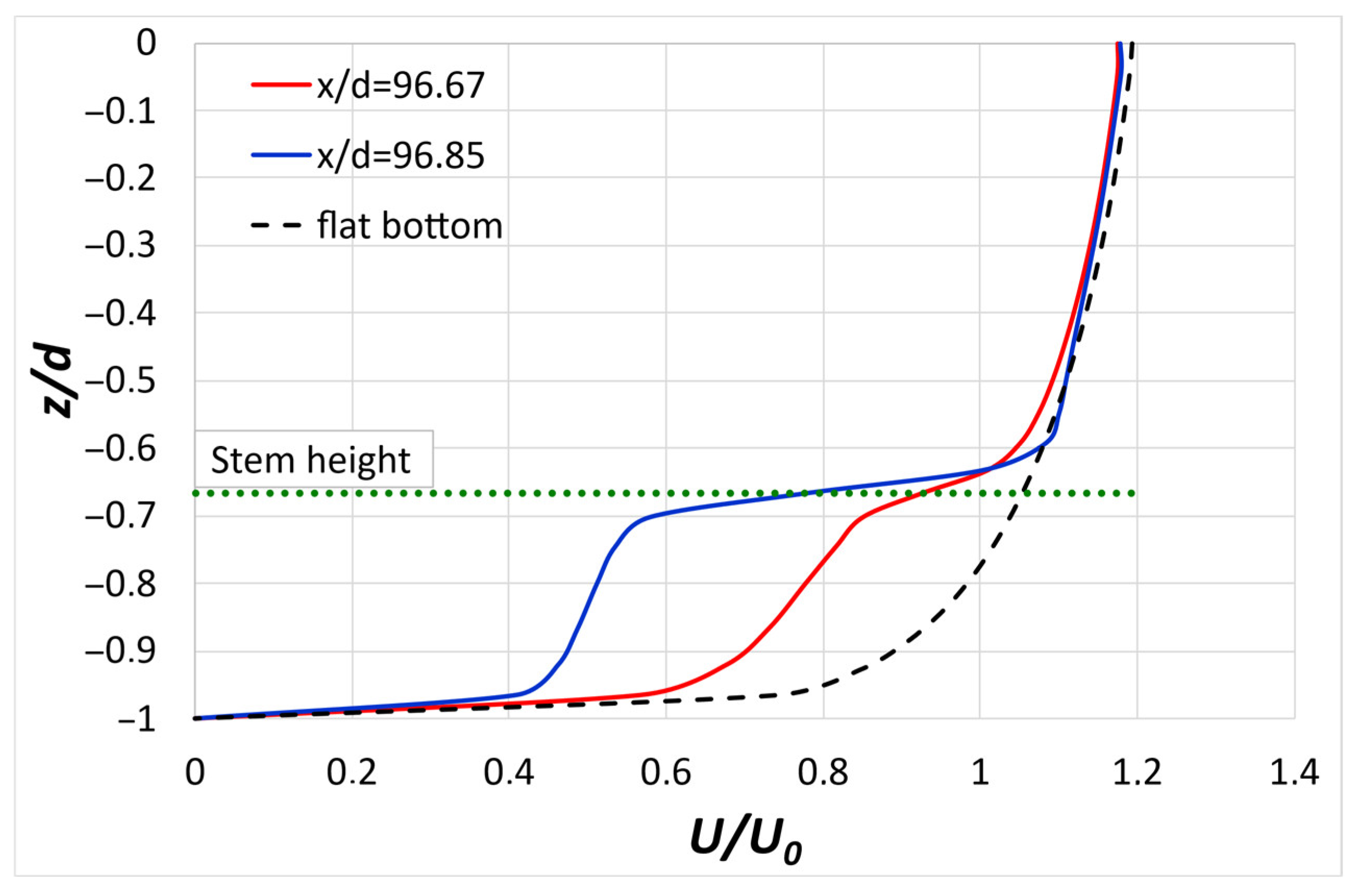
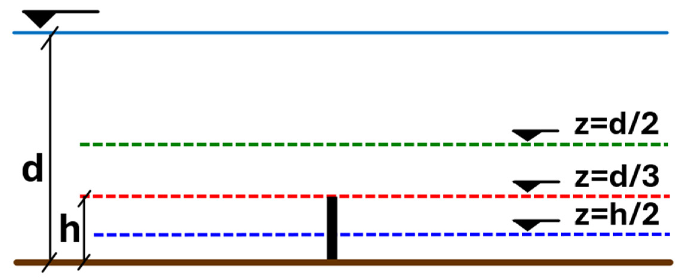
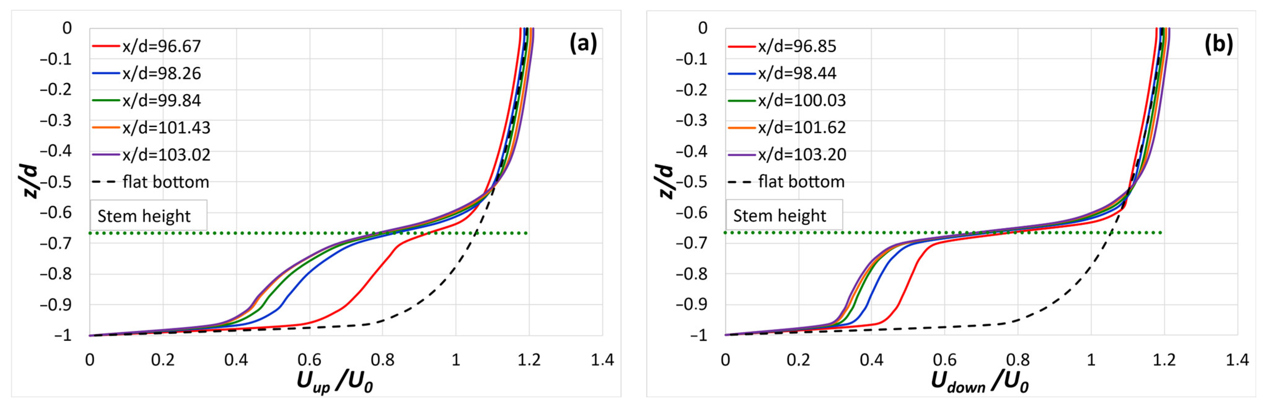
• The vertical distribution of streamwise velocity reveals significant reductions within the vegetated layer, particularly downstream of the stems. Above the vegetation height, velocity profiles closely adhere to the logarithmic law. The transition zone between vegetated and non-vegetated layers exhibits an inflection point, giving rise to shear-layer structures.
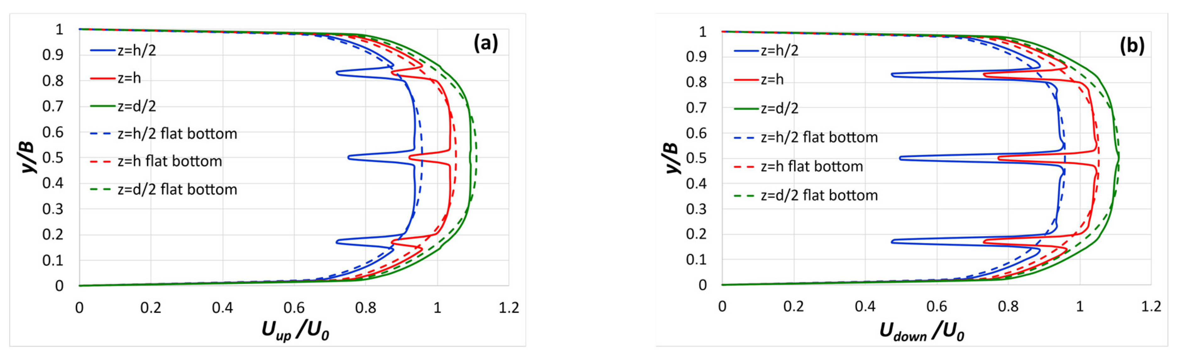
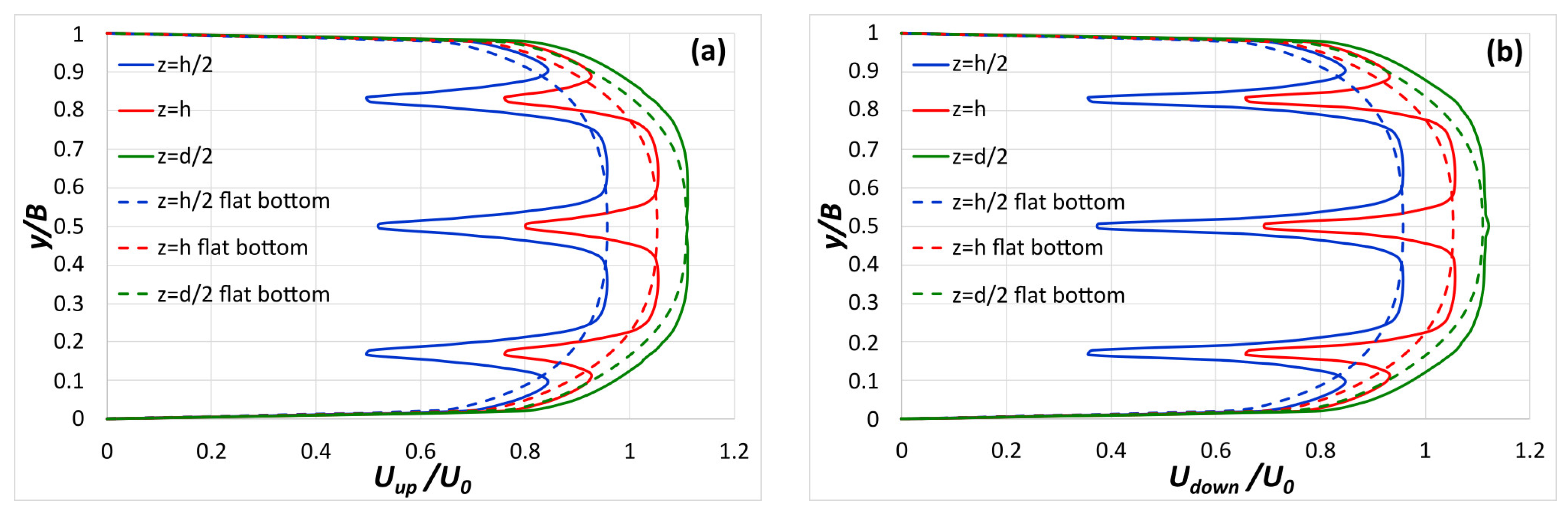
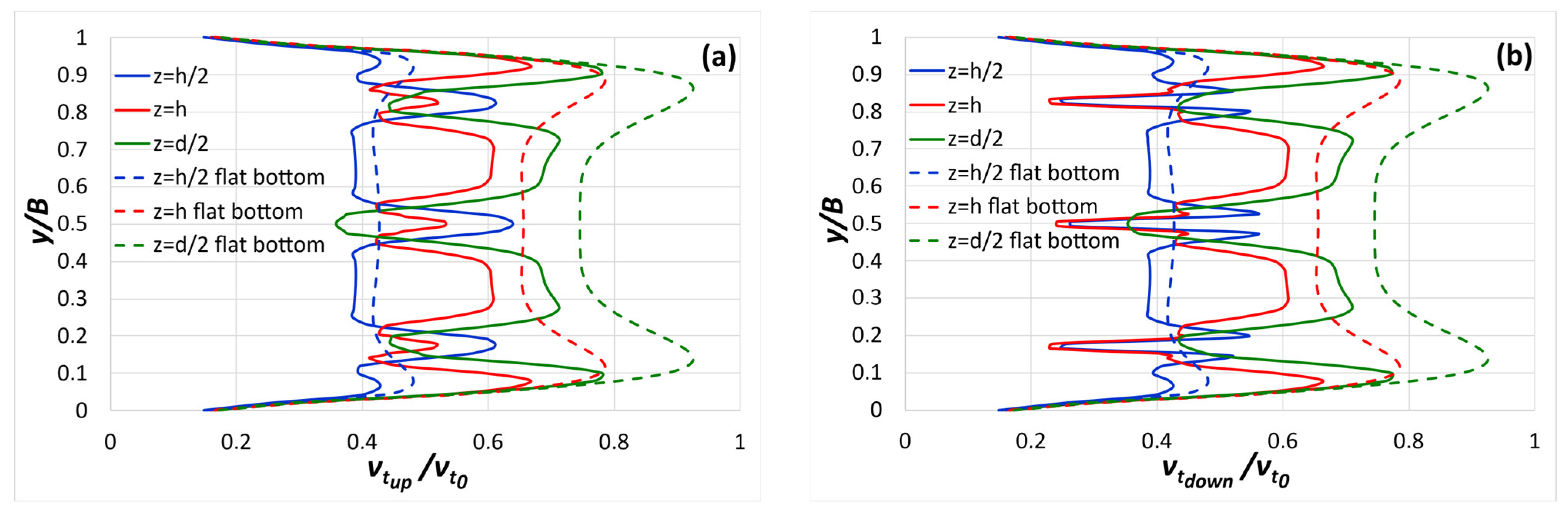
• Transverse velocity distributions indicate that the influence of vegetation is the strongest near the mid-stem height (z = h/2) and weakens progressively with depth. Velocity reductions are the most pronounced directly at the stem locations and persist downstream due to cumulative drag effects.
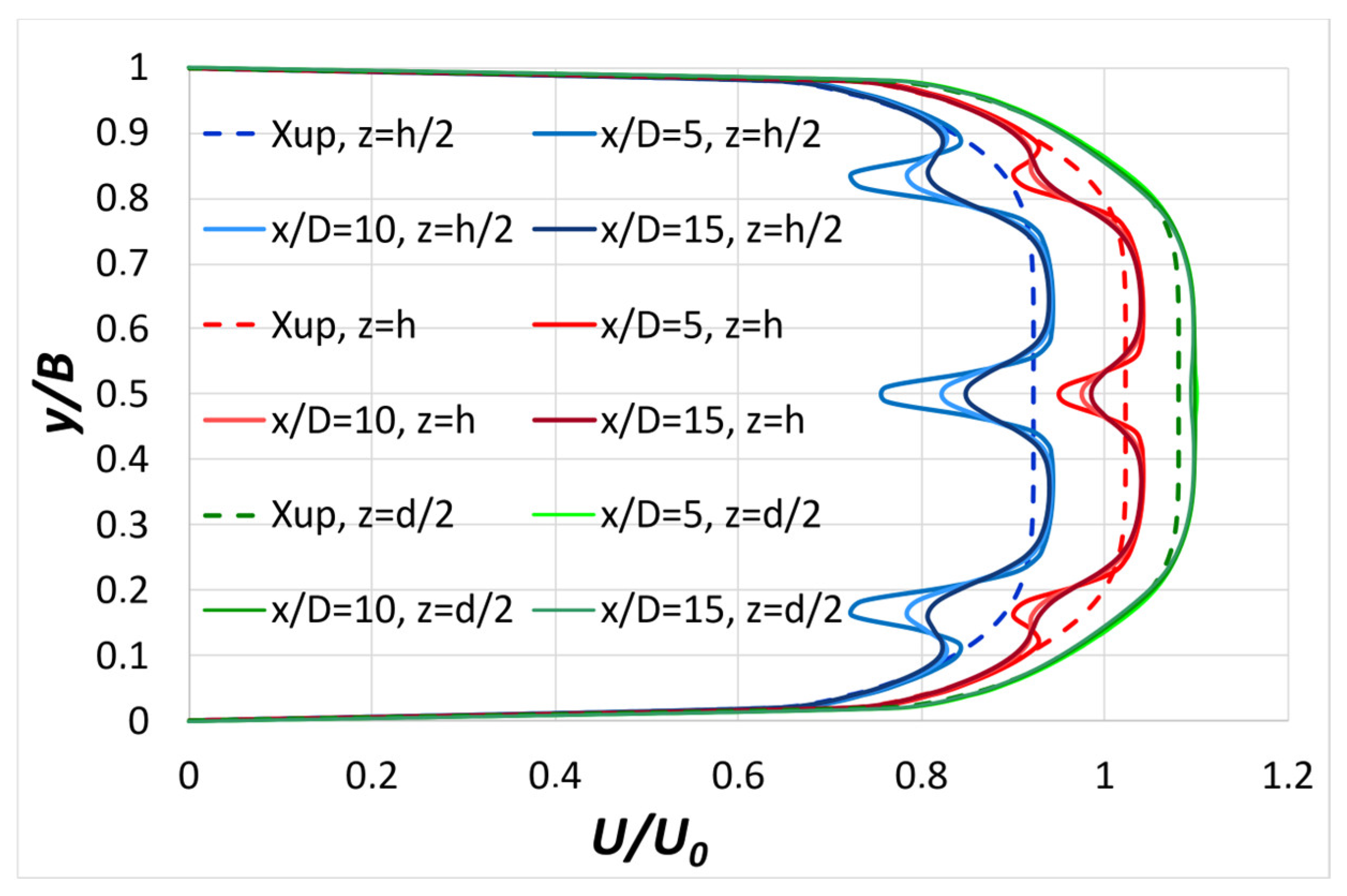
• In the second case, both upstream and downstream of the third stem series, repeatability is observed in the velocity profiles.
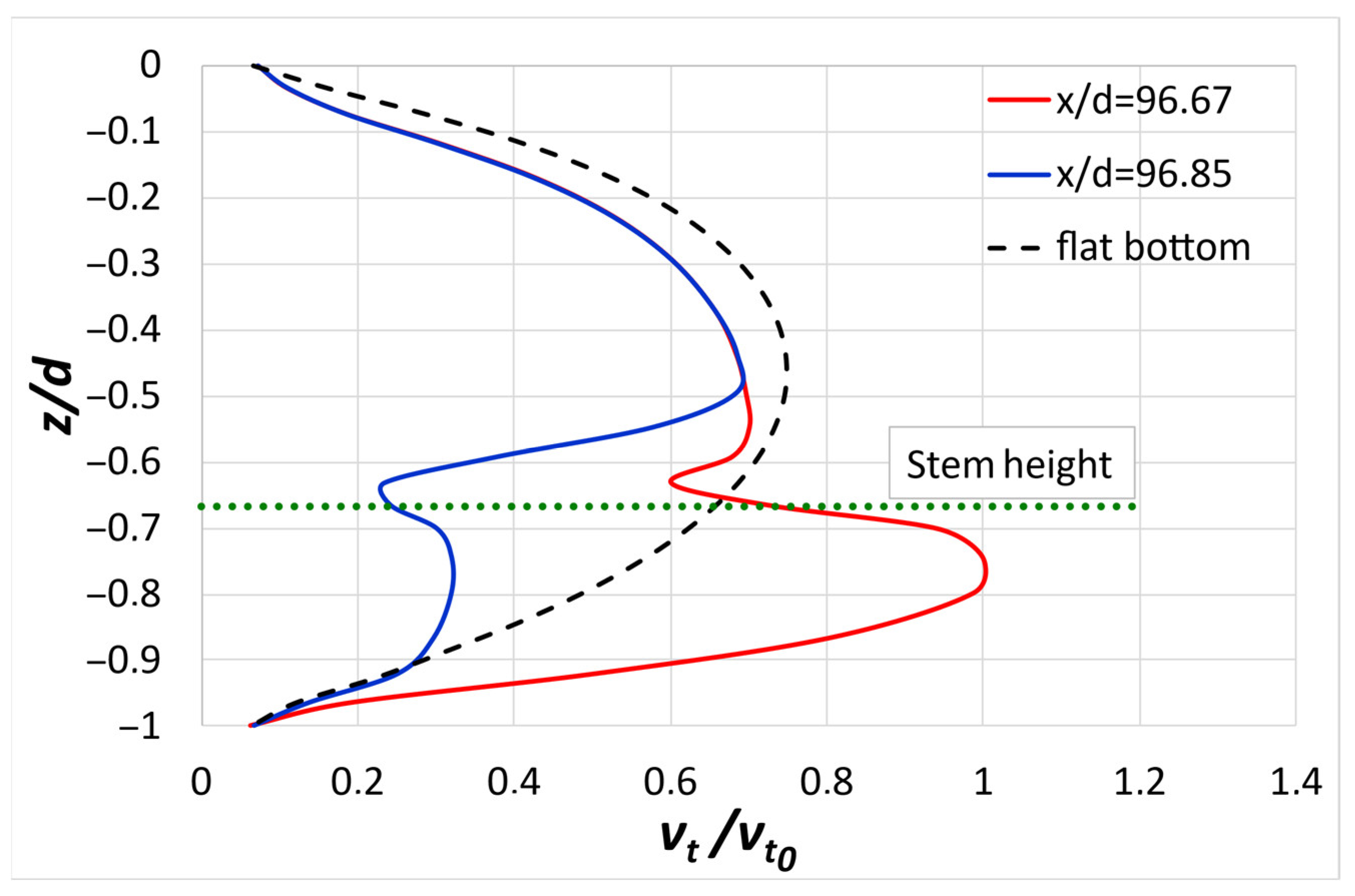
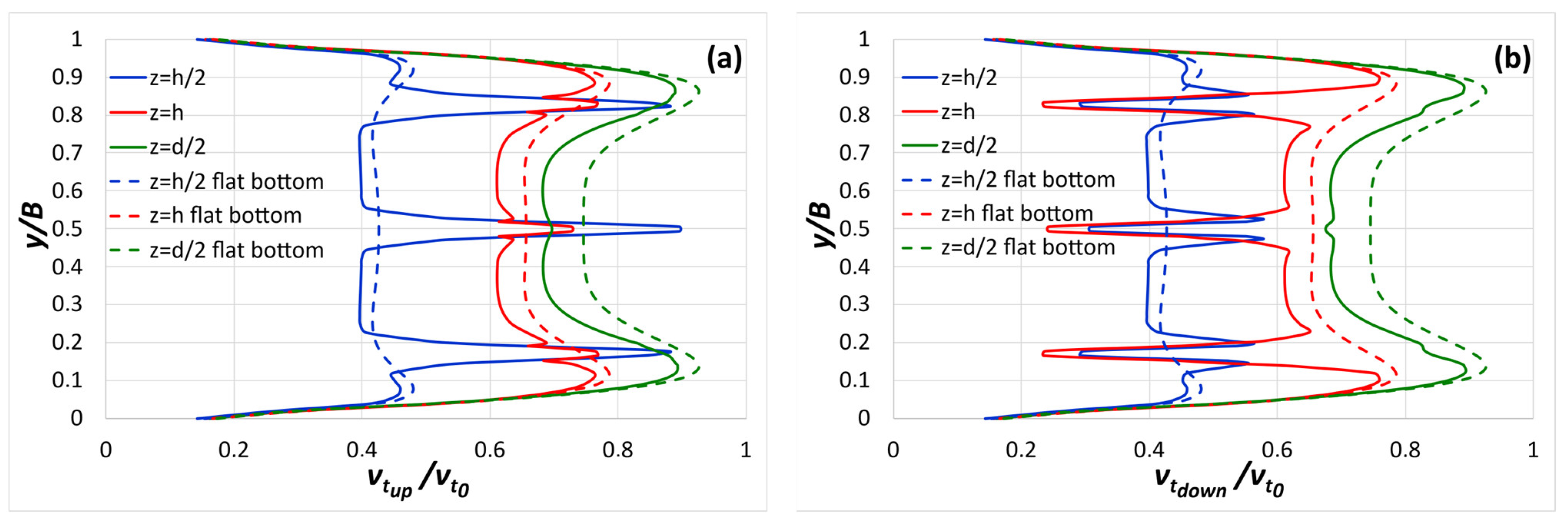
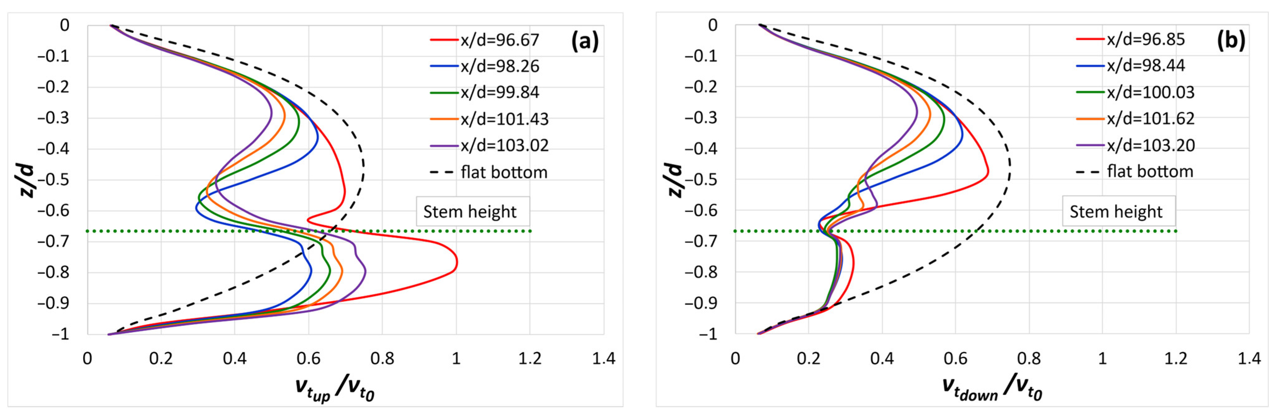
• The presence of submerged vegetation significantly modifies the turbulence structure. Eddy viscosity is generally increased upstream of stems due to flow separation and wake development, whereas it is reduced downstream, suggesting turbulence suppression in the wake zone.
• The largest enhancement in eddy viscosity occurs upstream of the first stem series in the parallel configuration, reflecting the abrupt onset of vegetative obstruction. Subsequent stem series experience reduced perturbations, further reinforcing the notion of flow field stabilization downstream.
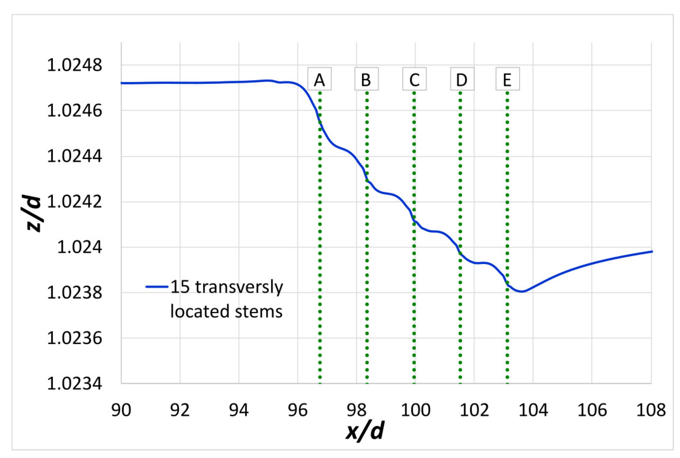
• In all scenarios, the subcritical flow regime results in localized free-surface depressions at stem locations and slight surface rises upstream of each series, in agreement with theoretical expectations for subcritical open-channel flow over submerged obstacles. Nevertheless, these free-surface fluctuations are considered negligible in relation to the normal depth for practical hydraulic applications in vegetated flows.

These findings contribute to a deeper understanding of vegetative flow resistance and support future efforts in ecohydraulic modeling, habitat design, and river restoration. The numerical results presented herein offer practical insights into the design of vegetated channels, floodplain management, and environmental hydraulics. Future research may expand this work by incorporating flexible vegetation models, validating simulations with experimental data, or coupling the flow field with sediment transport dynamics to assess long-term morphodynamic interactions in vegetated channels.

References

1. Nepf, H.; Ghisalberti, M. Flow and transport in channels with submerged vegetation. Acta Geophys. 2008, 56, 753–777. [Google Scholar] [CrossRef]
2. Fischer-Antze, T.; Stoesser, T.; Bates, P.; Olsen, N.R.B. 3D numerical modelling of open-channel flow with submerged vegetation. J. Hydraul. Res. 2001, 39, 303–310. [Google Scholar] [CrossRef]
3. Li, D.; Peng, Z.; Liu, G.; Wei, C. Flow Structures in Open Channels with Emergent Rigid Vegetation: A Review. Water 2023, 15, 4121. [Google Scholar] [CrossRef]
4. Zhang, J.; Zhang, S.; Wang, C.; Wang, W.; Ma, L. Flow characteristics of open channels based on patch distribution of partially discontinuous rigid combined vegetation. Front. Plant Sci. 2022, 13, 976646. [Google Scholar] [CrossRef] [PubMed]
5. Abdullahi, N.; Busari, A.O. Modeling Of Vegetated Open Channel Flow: A Review. Iconic Res. Eng. J. 2021, 4, 18–33. [Google Scholar]
6. O’Hare, M.T. Aquatic vegetation—a primer for hydrodynamic specialists. J. Hydraul. Res. 2015, 53, 687–698. [Google Scholar] [CrossRef]
7. Järvelä, J. Effect of submerged flexible vegetation on flow structure and resistance. J. Hydrol. 2005, 307, 233–241. [Google Scholar] [CrossRef]
8. Xu, Y.; Nepf, H. Measured and Predicted Turbulent Kinetic Energy in Flow Through Emergent Vegetation With Real Plant Morphology. Water Resour. Res. 2020, 56, e2020WR027892. [Google Scholar] [CrossRef]
9. Stone, B.M.; Shen, H.T. Hydraulic Resistance of Flow in Channels with Cylindrical Roughness. J. Hydraul. Eng. 2002, 128, 500–506. [Google Scholar] [CrossRef]
10. Nepf, H.M.; Vivoni, E.R. Flow structure in depth-limited, vegetated flow. J. Geophys. Res. Ocean. 2000, 105, 28547–28557. [Google Scholar] [CrossRef]
11. ANSYS. ANSYS FLUENT 2022 R1, User’s Guide; ANSYS Inc.: Canonsburg, PA, USA, 2022. [Google Scholar]
12. Launder, B.E.; Spalding, D.B. The numerical computation of turbulent flows. Comput. Methods Appl. Mech. Eng. 1974, 3, 269–289. [Google Scholar] [CrossRef]
13. Hirt, C.W.; Nichols, B.D. Volume of Fluid (VOF) Method for the Dynamics of Free Boundaries. J. Comput. Phys. 1981, 39, 201–225. [Google Scholar] [CrossRef]
14. Rajaratnam, N.; Nwachukwu, B.A. Flow Near Groin-Like Structures. J. Hydraul. Eng. 1983, 109, 463–480. [Google Scholar] [CrossRef]
15. Koutrouveli, T.I.; Dimas, A.A.; Fourniotis, N.T.; Demetracopoulos, A.C. Groyne spacing role on the effective control of wall shear stress in open-channel flow. J. Hydraul. Res. 2019, 57, 167–182. [Google Scholar] [CrossRef]
16. Elder, J.W. The dispersion of marked fluid in turbulent shear flow. J. Fluid Mech. 1959, 5, 544–560. [Google Scholar] [CrossRef]
17. Dimas, A.A.; Fourniotis, N.T.; Vouros, A.P.; Demetracopoulos, A.C. Effect of bed dunes on spatial development of open-channel flow. J. Hydraul. Res. 2008, 46, 802–813. [Google Scholar] [CrossRef]
18. Nezu, I.; Nakagawa, H. Turbulence in Open-Channel Flows, 1st ed.; IAHR Monograph Publisher: Balkema, Rotterdam, 1993; 293p. [Google Scholar]
19. Salaheldin, T.M.; Imran, J.; Chaudhry, M.H. Numerical Modeling of Three-Dimensional Flow Field Around Circular Piers. J. Hydraul. Eng. 2004, 130, 91–100. [Google Scholar] [CrossRef]
20. Anjum, N.; Ghani, U.; Ahmed Pasha, G.; Latif, A.; Sultan, T.; Ali, S. To Investigate the Flow Structure of Discontinuous Vegetation Patches of Two Vertically Different Layers in an Open Channel. Water 2018, 10, 75. [Google Scholar] [CrossRef]
21. Anjum, N.; Ali, M. Investigation of the flow structures through heterogeneous vegetation of varying patch configurations in an open channel. Environ. Fluid Mech. 2022, 22, 1333–1354. [Google Scholar] [CrossRef]
22. Amina; Tanaka, N. Numerical Investigation of 3D Flow Properties around Finite Emergent Vegetation by Using the Two-Phase Volume of Fluid (VOF) Modeling Technique. Fluids 2022, 7, 175. [Google Scholar] [CrossRef]
23. Gambi, M.; Nowell, A.; Jumars, P. Flume observations on flow dynamics in Zostera Marina (eelgrass) beds. Mar. Ecol. Prog. Ser. 1990, 61, 159–169. [Google Scholar] [CrossRef]
24. Alsina, V.S.; Cherian, R.M. Numerical investigation on the effect of flexible vegetation in open-channel flow incorporating FSI. ISH J. Hydraul. Eng. 2023, 30, 34–46. [Google Scholar] [CrossRef]
25. Liu, D.; Diplas, P.; Fairbanks, J.D.; Hodges, C.C. An experimental study of flow through rigid vegetation. J. Geophys. Res. Earth Surf. 2008, 113, F04015. [Google Scholar] [CrossRef]
Figure 1. Sketch focusing on the central part of the computational domain for the case with a parallel arrangement of five series of three equidistant, transversely located stems. The width of the channel as well as the normal depth of the flow are symbolized with B, and d, respectively.
Water 17 02156 g001
Figure 2. Vertical distribution of (a) longitudinal U-velocity and comparison with the logarithmic law and (b) eddy viscosity and comparison with the parabolic law [18] in the water layer for the flat-bottom case for two different meshes.
Water 17 02156 g002
Figure 3. Free-surface formation along the center of the channel due to the presence of three vegetative stems positioned transversely across the width of the channel and due to the presence of one individual stem at the channel’s center. The position of the middle stem is marked with A.
Water 17 02156 g003
Figure 4. Vertical distribution of longitudinal U-velocity in the water layer upstream (x/d = 96.67) and downstream (x/d = 96.85) of the central stem of the three-stem series compared with the corresponding distribution for the flat-bottom case.
Water 17 02156 g004
Figure 5. Vertical distribution of eddy viscosity in the water layer upstream (x/d = 96.67) and downstream (x/d = 96.85) of the central stem of the three-stem series compared with the corresponding distribution of eddy viscosity for the flat-bottom case.
Water 17 02156 g005
Figure 6. Visualization of flow depths in relation to normal flow depth and vegetation height.
Water 17 02156 g006
Figure 7. Distribution of longitudinal U-velocity in the transverse direction (a) upstream (x/d = 96.67) and (b) downstream (x/d = 96.85) of the stem series compared with the corresponding flat-bottom distributions at three different flow depths.
Water 17 02156 g007
Figure 8. Distribution of longitudinal U-velocity in the transverse direction for different locations downstream of the stem series, compared with the corresponding upstream distributions, at three different flow depths.
Water 17 02156 g008
Figure 9. Distribution of eddy viscosity in the transverse direction (a) upstream (x/d = 96.67) and (b) downstream (x/d = 96.85) of the stem series compared with the corresponding flat-bottom distributions at three different flow depths.
Water 17 02156 g009
Figure 10. Formation of free surface due to the presence of fifteen vegetative stems (one series of three stems in each of the positions A, B, C, D, and E) in the transverse direction.
Water 17 02156 g010
Figure 11. Vertical distribution of longitudinal U-velocity in the water layer (a) upstream and (b) downstream of the central stems from each series compared with the corresponding distribution for the flat-bottom case.
Water 17 02156 g011
Figure 12. Vertical distribution of eddy viscosity in the water layer (a) upstream and (b) downstream of the central stems from each series compared with the eddy viscosity distribution for the flat-bottom case.
Water 17 02156 g012
Figure 13. Distribution of longitudinal U-velocity in the transverse direction (a) upstream (x/d = 99.84) and (b) downstream (x/d = 100.03) of the third stem series compared with the corresponding flat-bottom distributions at three different flow depths.
Water 17 02156 g013
Figure 14. Distribution of eddy viscosity in the transverse direction (a) upstream (x/d = 99.84) and (b) downstream (x/d = 100.03) of the third stem series compared with the corresponding flat-bottom distributions at three different flow depths.
Water 17 02156 g014