Cascade Reservoir Outflow Simulation Based on Physics-Constrained Random Forest

Abstract

Accurate reservoir outflow simulation is crucial for water resource management. However, traditional machine learning-based simulation methods have not sufficiently considered the physical constraints of reservoir operation, which may lead to unrealistic issues such as negative outflows or water levels exceeding the reservoir’s own limitations. This study integrates physical constraints into the random forest (RF) model using the Sigmoid function, constructing a physics-constrained random forest model (PC-RF) for cascade reservoir outflow simulation. A stratified sampling strategy based on hydrological year types is used to create the training and validation datasets. The coefficient of determination (R²) and root mean square error (RMSE) are used to evaluate the model’s performance for medium- to long-term predictions of reservoir outflows on a 10-day time scale. Additionally, the mean decrease in impurity method is used to assess the importance of input features, thereby enhancing the model’s interpretability. The application the Yalong River cascade reservoir indicates that (1) compared to traditional RF, the PC-RF achieved significant breakthroughs, with an increase of 37.13% in the R² and a decrease of 60.04% in the RMSE when simulating outflows from the Lianghekou Reservoir, with all reservoirs maintaining an R² above 0.95, with no instances of unrealistic outcomes; (2) PC-RF effectively integrated historical operational patterns with top three features being previous period outflow, current inflow, and previous period inflow, providing interpretable insights for operational decision-making. The PC-RF model demonstrates high accuracy and practical potential in cascade reservoir outflow simulation, providing valuable applications for cascade reservoir management and water resource optimization.

1. Introduction

Reservoirs play a critical role in the global water resource management system, storing and controlling river runoff, and serving key functions such as flood prevention and drought mitigation, water supply security, hydropower generation, and ecological maintenance [1,2,3]. Global reservoir construction has developed rapidly, with the total storage capacity of large-scale reservoirs reaching approximately 7000–10,000 km³ [4,5]. Among these, China has constructed approximately 94,900 reservoirs of various types, with a total storage capacity of 807.7 km³ (as of the end of 2023, according to the 2023 National Water Resources Development Statistical Bulletin), which has effectively supported economic and social development and ecological environment protection.

As climate change intensifies and water resource demands grow, reservoir operation faces increasingly complex challenges, involving multi-time scale, multi-objective trade-offs, and emergency response mechanisms [6,7]. Reservoir outflow is a critical component of reservoir operation rules and a key control variable in water resource management, directly affecting downstream river hydrological processes, ecosystem health, and water resource utilization efficiency [8]. However, reservoir operation strategies vary significantly due to differences in hydrological characteristics (such as wet, normal, and dry years; flood and dry seasons), functional positioning (such as flood control, power generation, water supply, and irrigation), and management objectives (economic benefits, social benefits, and ecological benefits) [9,10]. This complexity makes accurately simulating reservoir operation rules and predicting outflow a significant challenge in water resource management.

Currently, reservoir operation simulation methods can be broadly categorized into two main types [11,12,13]. The first category comprises traditional methods that simulate reservoir outflows based on explicit operation charts, operation functions, and clear operation rules [14]. The primary limitation of traditional reservoir operation methods is their restricted generalizability. Moreover, operation practices for multi-purpose reservoirs often incorporate the experience and cognition of decision-makers, and these experiential and cognitive factors are difficult to fully generalize within operation rules. The second category of methods involves training machine learning algorithms using historical operation data to construct reservoir outflow models, which can effectively address the aforementioned problems [15].

In recent years, with the rapid development of artificial intelligence technology, machine learning (ML) models such as RF, recurrent neural network (RNN), and long short-term memory (LSTM) have gradually been applied to reservoir operation simulation [16,17,18,19]. For instance, Qie et al. [8] developed an RF model for predicting outflow from two reservoirs in Illinois, U.S.A. The results showed that the model performed excellently, with its accuracy and efficacy considered capable of effectively supporting reservoir management planning practices. Zhang et al. [20] employed three models—backpropagation neural network, support vector machine, and LSTM—to simulate the operation of the Gezhouba reservoir at monthly, daily, and hourly scales, with results indicating that the LSTM model achieved the highest accuracy.

As a black-box model, ML models lack inherent knowledge of reservoir operations, which may lead to problems such as generating unrealistic values (e.g., negative flow, water levels exceeding the maximum reservoir level), thereby limiting their ability to accurately simulate reservoir outflows [21]. To overcome these limitations, Zheng et al. [21] incorporated fundamental reservoir knowledge into the LSTM model’s loss function, including water balance, outflow boundaries, and other aspects, which can mitigate negative outflows and better capture reservoir operational characteristics. Similar research, including Chen et al. [22], Yu et al. [23], and Zheng et al. [24], demonstrates that physics-guided LSTM models significantly improve performance compared to traditional machine learning methods, providing an innovative approach to understanding reservoir operational behaviors. Qie et al. [8] pointed out that the random forest (RF) model is a powerful tool for simulating reservoir outflows; however, research on the coupling of physical constraints with RF models is still relatively scarce. This gap limits the ability of RF models to address the complex dynamic characteristics of reservoirs, thus underscoring the need for further exploration on how to effectively integrate physical knowledge into RF models to enhance their accuracy and reliability.

In the context of accelerating climate change and socio-economic development, the inconsistency between climatic hydrological conditions and human activities has become increasingly evident, with significant differences in outflow and water demand across different periods. However, the aforementioned studies continue to partition the training and validation data based on a temporal continuity strategy, making it challenging to simulate reservoir scheduling patterns under different hydrological conditions. This reliance on a temporal continuity strategy may limit the model’s performance in simulating reservoir outflows. To avoid such issues, some data partitioning algorithms that do not conform to temporal continuity criteria have been attempted in the construction of hydrological models, such as the DUPLEX algorithm [25], the SBS-S-N method [26], and the SBS-S-P algorithm [27]. However, for reservoir outflow simulation models, these algorithms disrupt the continuity of data during the reservoir scheduling period and increase the complexity of the models. Therefore, data partitioning methods based on hydrological year types are more suitable for reservoir outflow models. This approach ensures that both the training and validation periods include a sufficient quantity of data under different hydrological conditions while maintaining the continuity of inflow and outflow data within a given scheduling period.

This study contributes to the field in three main ways: (1) we develop a physics-constrained RF (PC-RF) model using a Sigmoid-based approach to embed operational constraints; (2) we propose a stratified sampling strategy based on hydrological year types to improve model generalizability; and (3) we assess model interpretability using input importance measures, linking physical features to decision-making insights.

2. Materials and Methods

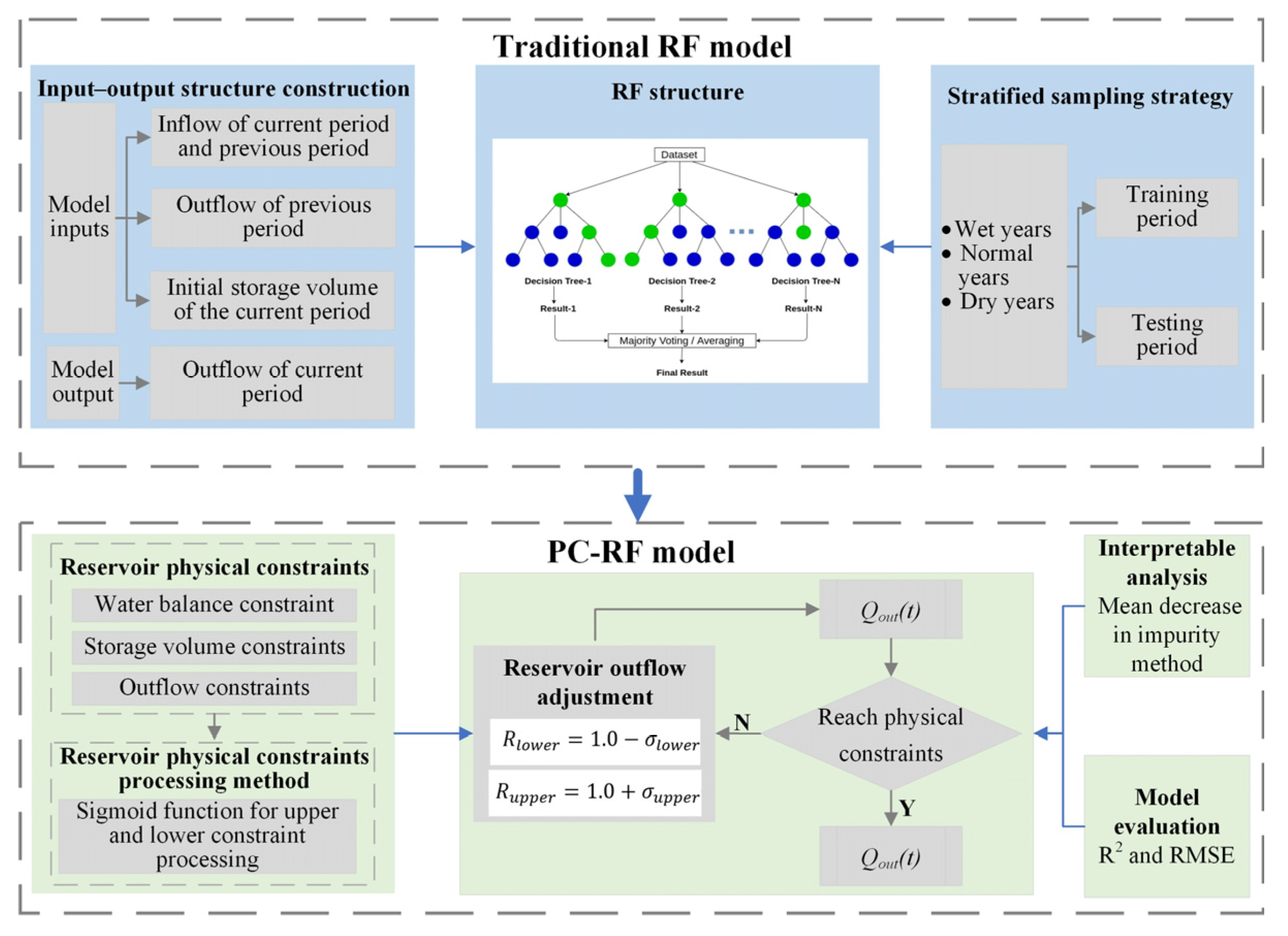
2.1. Physics-Constrained Random Forest Model (PC-RF)

As shown in Figure 1, to construct the PC-RF model for reservoir outflow simulation at the mid- to long-term time scale, we first defined the input–output structure of the model. Then, based on hydrological year types, a stratified sampling strategy was employed to divide the data, ensuring that the training and validation sets contained sufficiently representative wet, normal, and dry years. Next, the Sigmoid function was used to embed physical constraints into the RF model. Finally, the model’s performance was evaluated using two metrics, R² and RMSE, and the MDI method was applied for interpretability analysis of the model.

2.1.1. Input–Output Structure Construction

Reservoir inflow depends on upstream hydrological processes, and considering lag features, the reservoir’s current period and previous period inflow ($Q_t^{in}$ and $Q_{t-1}^{in}$) are used as input variables. Additionally, reservoir storage or reservoir water level are guiding factors for reservoir outflow, so the initial reservoir storage or initial reservoir water level are used as model input variables (these can be converted using the storage-level curve). Compared to reservoir water level, the correlation between changes in reservoir storage and reservoir outflow is more significant, so we select the initial storage volume of the current period ($V_{t-1}$) as an input variable for the model. Considering the continuity and experiential nature of reservoir scheduling, the previous period’s outflow ($Q_{t-1}^{out}$) is used as an input variable. We select the outflow of the current period ($Q_t^{out}$) as the output variable. After determining the input and output variables, the input-output structure was constructed based on machine learning algorithms such as RF, LSTM, etc., as shown in the following Equation (1):

$$Q_t^{out}=f(Q_t^{in},Q_{t-1}^{in},V_{t-1},Q_{t-1}^{out}),$$

(1)

where $f(·)$ represents the relationship between input and output variables, obtained through fitting by machine learning algorithms; the unit of t is ten-day.

2.1.2. Standsrd RF

RF is a powerful ensemble learning algorithm that improves overall model performance by constructing multiple independent decision trees and integrating their prediction results, and has been applied in the reservoir operation field [8]. Its core principle lies in diversity and ensemble: first, using bootstrap sampling to create multiple training subsets, ensuring differences in training data for each tree; second, randomly selecting feature subsets at each decision node for optimal splitting, further enhancing inter-tree diversity; finally, forming the ultimate prediction through voting (for classification problems) or averaging (for regression problems) across all decision trees, significantly improving model stability and accuracy.

2.1.3. Stratified Sampling Strategy

First, based on the inflow percentiles of the reservoir, the hydrological years are categorized into wet years (representing over 30% of inflow), normal years (30th–70th percentile), and dry years (the lower 30%). Subsequently, the datasets for wet, normal, and dry years are randomly sampled and divided into training and validation sets in an 8:2 ratio. Finally, the training sets for wet, normal, and dry years are combined to create a comprehensive training set, while the validation sets are merged to form an overall validation set. This approach ensures that both the training and validation sets contain a sufficient number of wet, normal, and dry years.

2.1.4. Physical Constraints and Processing Method

We incorporated readily available reservoir physical constraints (including water balance constraints, storage capacity constraints, and outflow constraints) into the ML model to improve its outflow simulation accuracy.

(1)

Water balance constraint

$$V_{i,t+1}=V_{i,t}+\left(Q_{i,t}^{in}-Q_{i,t}^{out}\right)∆t,$$

(2)

where $V_{i,t+1}$ and $V_{i,t}$ refer to the storage of reservoir i in the (t + 1)th and tth time steps, respectively, (m³); $Q_{i,t}^{in}$ represents the inflow to reservoir i at time t (m³/s), specifically including the inflow from upstream rivers; $Q_{i,t}^{out}$ denotes the outflow from reservoir i at time t (m³/s), which includes irrigation releases to nearby agricultural lands, ecological water, water released during power generation at hydropower stations, and flow discharged through spillways and other drainage structures. It is worth noting that while evapotranspiration and seepage losses are significant outflows from the reservoir, this study primarily focuses on the outflow dynamics at the mid- to long-term time scale, and therefore, these factors are not directly included in the calculation of $Q_{i,t}^{out}$.

(2)

Storage volume constraints

$$V_{i,t}^{lower}\le V_{i,t}\le V_{i,t}^{upper},$$

(3)

where $V_{i,t}^{lower}$ and $V_{i,t}^{upper}$ are the lower and upper storage of reservoir i at time t, respectively (m). In this study, the lower limit storage capacity is set as dead storage, and the flood control storage capacity is used as the upper limit constraint during the main flood season (24th–27th ten-day periods), while the storage capacity at normal pool level is applied as the constraint during the non-flood season.

(3)

Outflow constraints

$$Q_{i,t}^{out, l}\le Q_{i,t}^{out}\le Q_{i,t}^{out,u},$$

(4)

where $Q_{i,t}^{out, l}$ and $Q_{i,t}^{out,u}$ are the lower and upper outflow of reservoir i at time t, respectively (m).

We adopt a smooth constraint mechanism, using Sigmoid function to process reservoir constraint conditions, which has significant advantages over loss function methods: First, the Sigmoid function can rigidly ensure that the final output 100% satisfies physical constraint conditions, while the loss function method can only perform “soft constraints” through penalty terms and cannot absolutely guarantee constraint satisfaction; Second, the smooth constraint mechanism implemented by the Sigmoid function avoids the sudden change problem of hard constraints, ensuring a continuous and smooth adjustment process, whereas constraint terms in loss functions often lead to gradient discontinuity, affecting model convergence; meanwhile, the Sigmoid function can automatically adjust constraint strength according to the degree of violation, providing an intelligent adaptive constraint response mechanism. Specific processing steps: The Sigmoid function calculates the expected storage volume for the next time period through water balance principles based on actual operational characteristic parameters of the reservoir. When the simulated storage volume exceeds the upper limit, the adjustment ratio is calculated through the sigmoid smoothing factor of the upper constraint to increase reservoir outflow; When the simulated storage volume falls below the lower limit, the adjustment ratio is calculated through the sigmoid smoothing factor of the lower constraint to reduce reservoir outflow.

Upper constraint processing:

$${\sigma }_{upper}={\displaystyle \frac{1}{1+e^{-\frac{∆V_{excess}}{\alpha }}}},$$

(5)

where ${\sigma }_{upper}$ is the sigmoid smoothing factor for upper limit constraint; $∆V_{excess}$ is the excess storage volume; $\alpha$ is the scaling parameter, set to 100 in this study.

Lower constraint processing:

$${\sigma }_{lower}={\displaystyle \frac{1}{1+e^{-\frac{∆V_{deficit}}{\beta }}}},$$

(6)

where ${\sigma }_{lower}$ is the sigmoid smoothing factor for lower limit constraint; $∆V_{deficit}$ is the deficit storage volume; $\beta$ is the scaling parameter, set to 100 in this study.

Reservoir outflow adjustment ratio:

$$R_{upper}=1.0+{\sigma }_{upper},$$

(7)

$$R_{lower}=1.0-{\sigma }_{lower},$$

(8)

where $R_{upper}$ is the reservoir outflow adjustment ratio for upper limit constraint (≥1.0, increasing outflow); $R_{lower}$ is the reservoir outflow adjustment ratio for the lower limit constraint (0–1.0, reducing outflow).

2.2. Reference Model

Given the advantages of bidirectional long short-term memory networks (BiLSTMs) in reservoir outflow modeling, we concurrently develop a BiLSTM model that considers physical constraints (PC-BiLSTM) as a reference model. LSTM network is a specialized recurrent neural network architecture designed for sequence data processing, solving the gradient vanishing problem of traditional RNNs through an ingenious gating mechanism, and is widely applied in hydrological time series problems [18,22]. Its core lies in its sophisticated internal structure, featuring a cell state channel running through the entire network and three critical gating mechanisms: the input gate controls the extent of new information entering the cell state, the forget gate determines which historical information to discard, and the output gate manages the volume of output information from the current state. This design enables LSTM to long-term preserve important information, selectively forget irrelevant information, and demonstrate excellent performance in long sequence modeling. The BiLSTM further extends this architecture, comprising two independent LSTM layers with opposite directions: the forward layer processes the sequence chronologically, while the backward layer processes it in reverse order, ultimately merging the outputs of both layers. Therefore, this study includes a total of four machine learning models for reservoir outflow simulation, namely RF, PC-RF, BiLSTM, and PC-BiLSTM. Details of the model parameter settings can be found in the Supplementary Materials (Table S1).

2.3. Model Evaluation

Two statistical indices are selected to evaluate the accuracy of models: R² and RMSE. The value range of R² is typically between 0 and 1, with values closer to 1 indicating that the model explains a greater proportion of variance and thus provides a better fit. R² can also be negative, indicating that the model predictions are worse than simply predicting the mean value. Lower RMSE values indicate smaller prediction errors and better model fitting performance. The specific formulas of each consistency statistical index are as follows:

$${\mathrm{R}}^2=1-{\displaystyle \frac{\sum _{t=1}^N(Q_{obs,t}{-Q_{sim,t})}^2}{\sum _{t=1}^N(Q_{obs,t}{-{\overline{Q}}_{obs,t})}^2}},$$

(9)

$$\mathrm{R}\mathrm{M}\mathrm{S}\mathrm{E}=\sqrt{{\displaystyle \frac{1}{N}}\sum _{t=1}^N{Q}_{obs,t}{-Q_{sim,t})}^2},$$

(10)

where $Q_{obs,t}$ and $Q_{sim,t}$ denote the observed and simulated reservoir outflow, respectively; ${\overline{Q}}_{obs,t}$ denotes the mean observed outflow; $N$ represents the number of samples.

2.4. Mean Decrease in Impurity Method

The MDI method is an intrinsic feature of the RF model that quantifies the importance of each feature by measuring the contribution of a feature to the model’s predictive accuracy. The basic principle is that, during the construction of decision trees in the forest, the algorithm evaluates how well each feature splits the data, reducing impurity (e.g., Gini impurity or entropy) in each node. The total decrease in impurity brought by a specific feature across all trees in the forest is then accumulated. The more a feature contributes to reducing impurity in the splits, the higher its importance score. This method allows for a clear understanding of which features are most influential in the model’s predictions, enhancing interpretability.

3. Case Description

3.1. Study Area

The Yalong River Basin is located in the southeastern part of the Tibetan Plateau and is one of the eight major tributaries of the Yangtze River. It belongs to the western Sichuan Plateau climate zone, with distinct dry and wet seasons. The flood season spans from June to October, while the dry season extends from November to May of the following year. The hydrological year is defined from November to October of the following year. The main stream is 1535 km long, with a natural elevation drop of 3192 m. It is the third-largest hydropower base in China’s energy strategic layout, with a developable installed capacity of 30 million kW and a potential annual power generation of 150 billion kWh. Currently, the total installed capacity reaches 19.2 million kW, including reservoirs with multi-year (Lianghekou, LHK), yearly (Jinping I, JP1), and seasonal (Ertan, ET) regulation capabilities. The topological structure and main characteristic parameters of the cascade reservoirs are shown in Figure 2 and

Table 1. The information on the three reservoirs in the Yalong River Basin.

Reservoir	Normal Pool Level (m)	Flood Control Level (m)	Dead Water Level (m)	Storage Capability at Normal Pool Level (108 m3)	Storage Capability at Flood Control Level (108 m3)	Dead Storage (108 m3)	Reservoir Capability	Installed Capacity (MW)
LHK	2865	2845.9	2785	101.5	81.5	35.9	multi-year	3000
JP1	1880	1859.0	1800	77.6	61.6	28.4	yearly	3600
ET	1200	1190.0	1155	57.9	48.5	24.0	seasonal	3300

.

3.2. Data

This study focuses on the mid- to long-term outflow simulation of cascade reservoirs, typically analyzed on a monthly or 10-day scale. Thus, we collected 10-day outflow, inflow, and reservoir storage data (1958–2021) for the LHK, JP1, and ET reservoirs from the Bureau of Hydrology, Changjiang Water Resources Commission. It is worth noting that the construction and operation of these three reservoirs occurred relatively late, and the outflow data for several years were derived from the reservoir design phase, assuming them to be observed values, specifically LHK (1958–2021), JP1 (1958–2014), and ET (1958–2000). The static characteristic parameters of the three reservoirs were compiled, including normal pool level, flood control level, dead water level, and their corresponding storage capacities (Table 1).

4. Results

4.1. Dataset Sampling

Based on inflow percentiles, we classified the 64-year period of LHK reservoir data into wet years (19 years), normal years (26 years), and dry years (19 years). The statistical analysis of inflow shows that the mean inflow is 681.77 m³/s, the standard deviation (SD) is 126.51 m³/s, the maximum (Max) inflow is 985.53 m³/s, and the minimum (Min) inflow is 451.64 m³/s. Wet years (blue markers) have annual inflow mainly concentrated in the range of 700–1000 m³/s, occupying the upper 30th percentile of inflow; normal years (green markers) have annual inflow between 600 and 750 m³/s, representing the middle 40th percentile; dry years (red markers) have relatively low annual inflow, mainly distributed in the 450–600 m³/s range, corresponding to the lower 30th percentile. We randomly sampled and divided the data from different hydrological years into training and validation sets. The distribution of data points in the training period (represented by circles) and the validation period (represented by half circles) along the time axis is shown in Figure 3, ensuring that each type of hydrological year in both the training and validation sets is adequately represented. Additionally, it can be seen that the inflow time series of the LHK reservoir exhibits significant interannual variability, with substantial differences in inflow between different hydrological year types, providing a strong practical basis for stratified sampling.

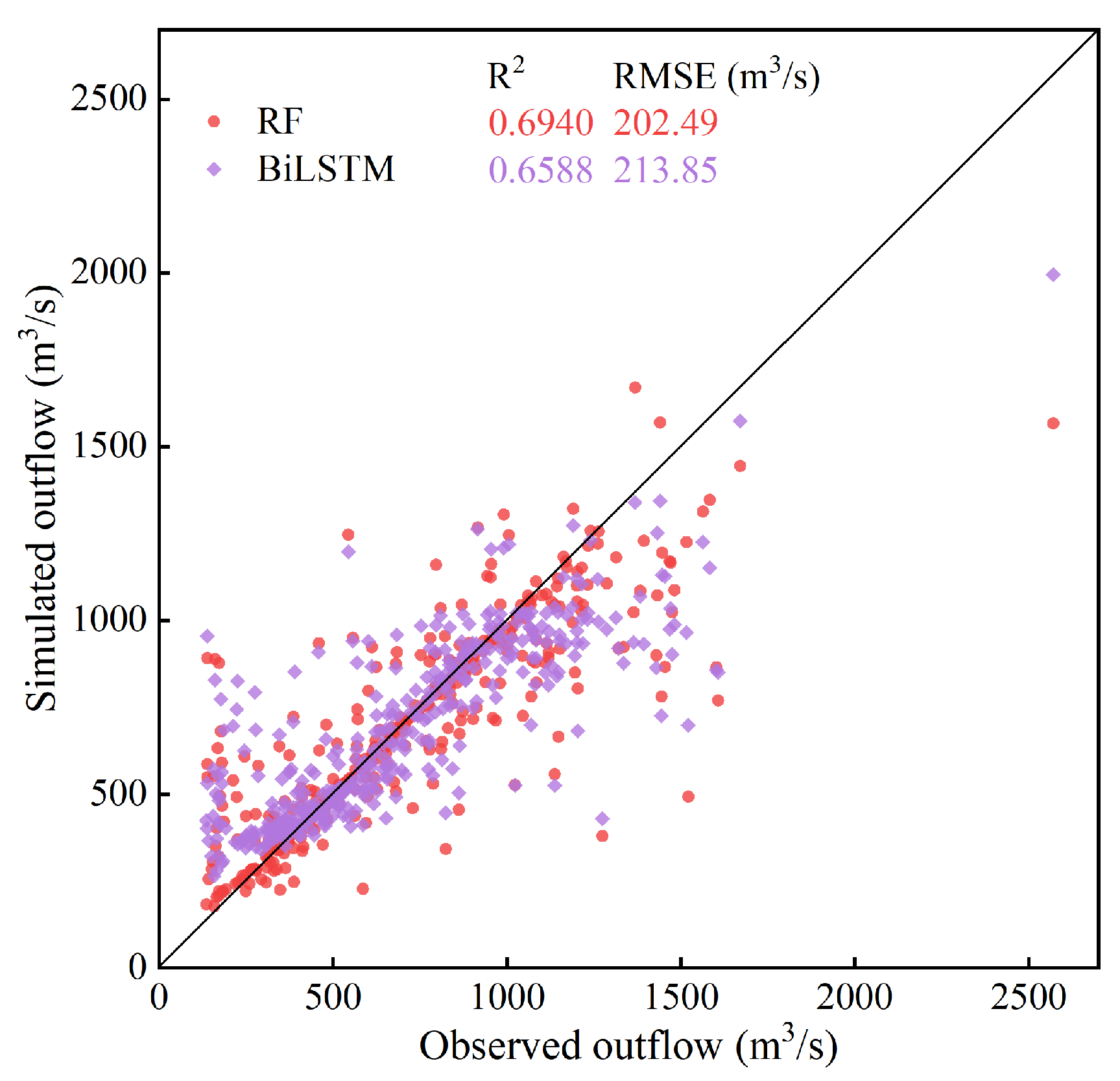
4.2. Assessment of RF and BiLSTM Models Without Physical Constraints

Figure 4 illustrates the performance comparison of the unconstrained RF and BiLSTM in simulating outflow for the LHK reservoir. The results indicate that the RF model achieves an R² of 0.6940 and an RMSE of 202.49 m³/s, while the BiLSTM model has an R² of 0.6588 and an RMSE of 213.85 m³/s. Although the RF model performs slightly better than the BiLSTM, both exhibit low predictive accuracy, challenging the previous conclusion that LSTM outperforms in time series simulation. This may be attributed to two potential factors: first, reservoir dispatch decisions largely depend on current hydrological conditions and downstream water demand rather than long-term historical sequences, and are significantly influenced by subjective factors; second, this study adopts a ten-day time scale, and the relatively limited sample size is inadequate to fully realize the potential of BiLSTM. This also underscores that model selection should be tailored to specific application contexts rather than solely based on model type.

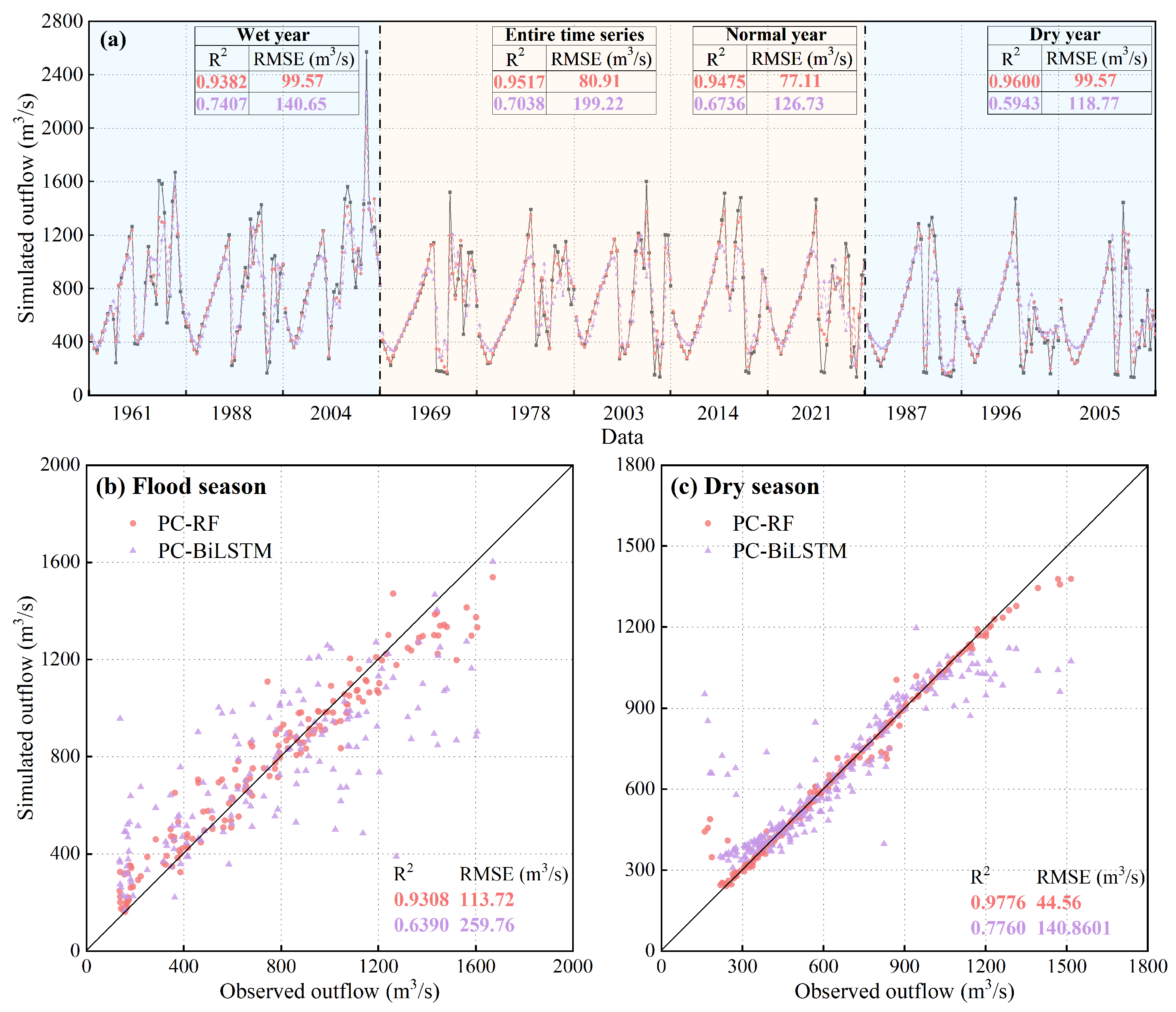
4.3. Assessment of PC-RF and PC-BiLSTM Models

Given the advantages of the bidirectional long short-term memory network (BiLSTM) in reservoir outflow modeling, we simultaneously developed a physically constrained BiLSTM model (PC-BiLSTM) as a reference model. Taking the Lianghekou Reservoir as an example, we conducted a comparative analysis of the performance of PC-RF and PC-BiLSTM. Figure 5 displays comparative results of the physics-constrained RF model (PC-RF) and physics-constrained BiLSTM model (PC-BiLSTM) in reservoir outflow prediction. PC-RF model demonstrates markedly superior overall performance, with a total R² of 0.9517 and RMSE of 80.91 m³/s. Across different hydrological years, PC-RF maintained high accuracy, performing exceptionally well in dry years (R² = 0.9600, RMSE = 64.65 m³/s) and maintaining high precision in wet years (R² = 0.9382, RMSE = 99.57 m³/s). In contrast, the PC-BiLSTM model performed poorly across all year types, with significantly reduced accuracy in dry years (R² of only 0.5943). Across different hydrological periods, the PC-RF model consistently maintained high precision, excelling in both flood and dry seasons, while the PC-BiLSTM model demonstrated weak performance, particularly during the flood season (R² = 0.6390, RMSE = 259.76 m³/s). The learning curve of the PC-BiLSTM model can be seen in Figure S1 in the Supplementary Materials, and no overfitting phenomenon is present. We further compared the reservoir storage predictions of the two models using water balance constraints (see Figure 6). It is evident that both models demonstrate good performance (R² > 0.9). The primary reason for this is that the LHK reservoir has a very large storage capacity, with a normal water level corresponding to a volume of 101.5 $\times$ 10⁸ m³. As a result, the impact of outflow errors transmitted to the storage variable is significantly reduced, enhancing the stability and accuracy of the prediction models. Overall, the PC-RF model exhibited exceptional performance, accurately capturing flow peak and low-value variations. This demonstrates the significant advantages of combining random forest algorithms with physical constraints in reservoir dispatch simulation, providing more reliable technical support for practical applications.

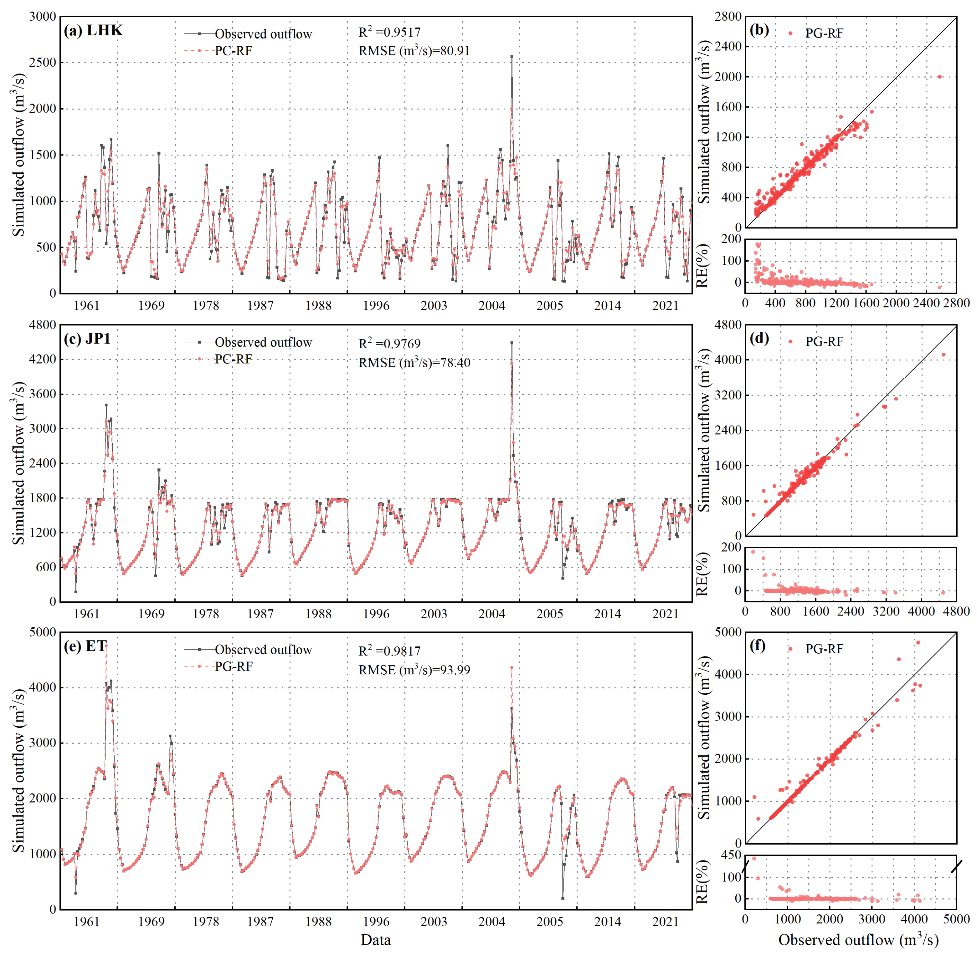
4.4. Assessment of PC-RF Model in Simulating Outflow for Cascade Reservoirs

Here, we applied PC-RF to simulate outflows in the cascade reservoirs of the Yalong River Basin. Figure 7 demonstrates the performance of the PC-RF in outflow simulation for the LHK, JPI, and EF reservoirs in the Yalong River Basin. By comparing observed and simulated outflows, the model exhibits remarkable accuracy in the validation period, with R² values exceeding 0.95 for all three reservoirs and RMSE of 80.91, 78.40, and 93.99 m³/s, respectively. The relative error (RE) distribution plot (Figure 7b,d,f) reveals that most data points are concentrated within a ±10% error range, indicating that the model can control outflow simulation errors within an extremely small scope in the majority of cases. Notably, in the low outflow interval, RE fluctuations are more significant, showing a tendency for overestimation, with the maximum RE reaching 434.42% (for the ET). This abnormal relative error occurred in the early storage phase of the 2005 flood season (late July). That year was a drought year, and the inflow amount was only 793.94 m³/s, which is the historical minimum for that period and far below the multi-year average (2418.90 m³/s) for the same time frame. Therefore, due to insufficient inflow and storage requirements, the designated outflow for that period was set at 206.70 m³/s, which is also the historical minimum for that period, significantly lower than the multi-year average (2196.71 m³/s). Such a rare situation is extraordinary and was not included in the training data, causing the PC-RF model to be unable to simulate it effectively. Fortunately, the frequencies of high errors (exceeding ±50% RE) for the three reservoirs are all low, at 4.55%, 1.01%, and 0.77%, respectively, and they all exhibit overestimations, meaning the predicted values are greater than the observed values. The overall error remains within an acceptable range. This demonstrates the effectiveness and reliability of the PC-RF model in simulating outflows of the Yalong River cascade reservoirs, showcasing its capability to capture long-term reservoir outflow dynamic variations.

5. Discussion

5.1. The Enhanced Effect of PC-RF Model

Accurately simulating the operation of cascade reservoirs in a basin, while simultaneously considering hydrological and reservoir physical characteristics, remains a significant challenge [23]. Compared with models without physical constraints, the PC-RF model significantly improved simulation performance, with R² increasing by 37.13% and RMSE reducing by 60.04%. Additionally, the p-value of the paired t-test is 0.0076, further validating the statistical significance of the error differences between the two models. We provide additional prior knowledge by introducing water balance constraints, storage capacity constraints, and outflow constraints. The PC-RF model’s enhanced features considered reservoir safe operation characteristics, increasing the feature count from 20 to 49 for the flood season model and 37 for the dry season models. Specifically, flood season features include distance to flood control water level, distance to flood control reservoir capacity, flood season storage ratio, and exceedance of flood control limits. Moreover, based on normal pool level, dead water level, and corresponding reservoir capacities, the model constructed a simplified linear reservoir capacity–water level relationship, making the model more aligned with actual operational rules and significantly improving the accuracy of reservoir outflow simulation. Our findings are consistent with the perspectives of Shen et al. [28] and Tripathy et al. [29], which suggest that integrating physical constraints with machine learning models generates more generalized solutions that can effectively leverage their strengths to address hydrological challenges.

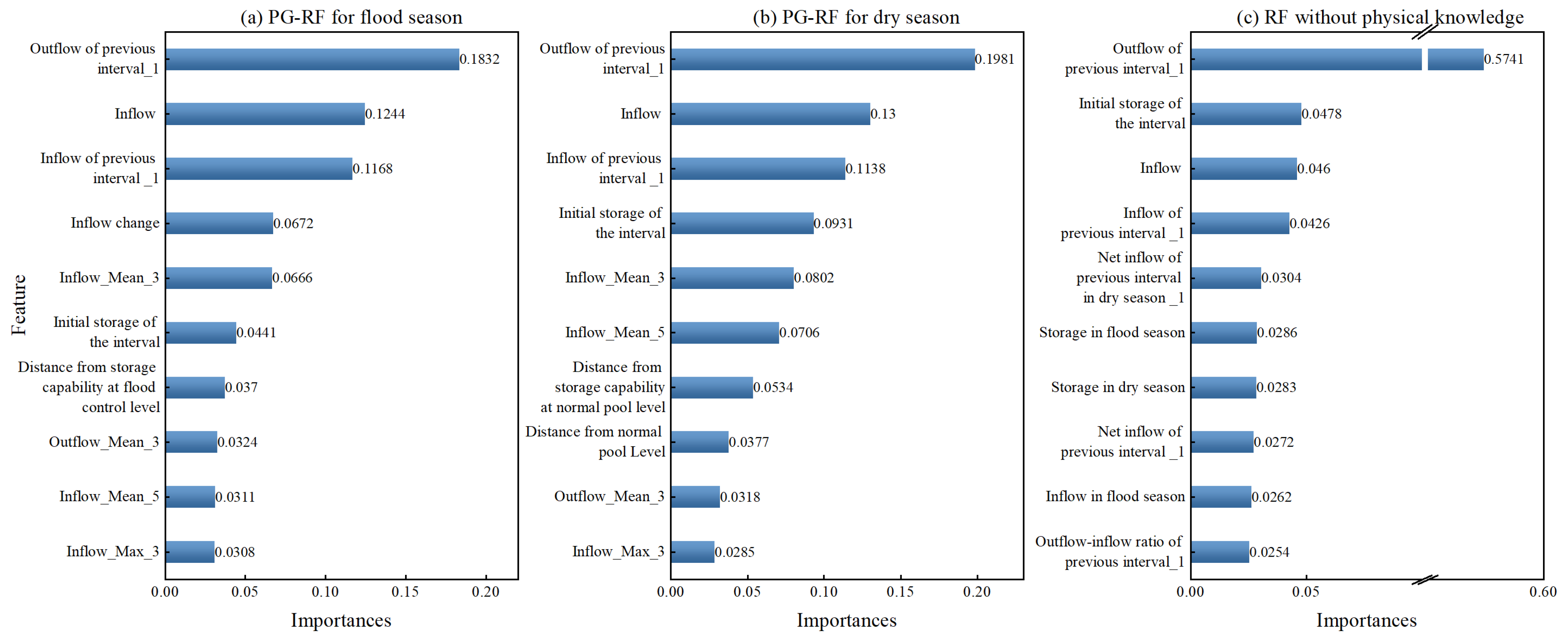
5.2. An Interpretable Analysis of the PC-RF Model

Further, based on the built-in feature importance calculation mechanism of the RF model, we used the mean decrease in impurity (MDI) method to quantitatively analyze feature importance and identify the most influential factors for outflow prediction [30]. Figure 8 shows the top 10 features and their importance. It can be observed that the PC-RF model for flood and dry seasons has consistent top three features: outflow of previous interval_1 (18.32%, 19.81%), inflow (12.44%, 13%), and inflow of previous interval_1 (11.68%, 11.38%). These features are particularly important in current reservoir management because inflows and outflows directly determine the strategies for water storage and release. During the flood season, the feature” Distance from storage capability at flood control level” (3.7%) is especially critical as it directly reflects the gap between the current water level and the safe flood control level. Managers need to pay close attention to this feature in order to adjust the reservoir’s storage strategy and outflow rates. Once the water level is monitored to be approaching the flood control level, managers must respond quickly and may choose to increase outflows to lower the water level, thus reducing the risk of flooding and ensuring the safety of downstream areas. In the dry season, the feature “ Distance from storage capability at normal pool level” (5.34%) becomes an important reference for guiding storage decisions and optimizing water resource utilization. By monitoring this distance, managers can assess whether the reservoir’s water level is sufficient to adequately meet future water needs, especially during drought periods. When the water level is too low, managers need to take corresponding measures to reduce outflows to ensure that downstream water needs can be met.

Additionally, we found that the PC-RF model’s feature enhancement approach constructs a more comprehensive feature space: the original four variables (46.85% in flood season, 53.50% in dry season) contribute comparably to the newly generated features. This demonstrates the RF model’s unique ability to capture complex potential dynamic characteristics of the hydrological system through implicit feature interaction, non-linear mapping, and entropy reconstruction. This feature enhancement approach not only expands the model’s information dimensions but also endows the model with deeper system insights, elevating it from data fitting to a profound understanding of the hydrological system’s intrinsic mechanisms, significantly improving the model’s interpretability and simulation accuracy.

However, the RF model without physical constraints exhibits a clear dependency imbalance, with the “Outflow of previous interval_1” becoming the dominant feature with an absolute advantage of 57.41%, far exceeding the combined influence of other factors. This feature importance distribution explains why the model without physical constraints performs poorly—it excessively relies on historical scheduling patterns rather than fundamental hydrological physical laws, resulting in limited generalization capabilities when facing new situations, especially potentially generating physically unreasonable simulation results under extreme hydrological conditions, unable to provide reliable reservoir scheduling decision support.

5.3. Limitations

Although the cascade reservoir outflow simulation method proposed in this study has achieved good results, the following limitations still exist: First, when reservoir outflows are small (especially under low flow conditions during dry periods), the model’s simulation accuracy is relatively poor. This is primarily due to the small proportion of small outflow data in the training set and the limited capability of physical constraints to represent conditions under extremely low flows. To address this issue, future research could consider employing data augmentation techniques, including synthesizing small outflow cases, to enhance the model’s predictive ability under low flow conditions. Additionally, exploring transfer learning methods that utilize data obtained from other regions or conditions could improve the model’s adaptability in low-flow situations. Second, the model’s performance is highly dependent on the quality and completeness of long-term historical data, limiting its applicability for reservoirs lacking long-term observation records. To improve this, future research could integrate remote sensing technology and climate prediction data to construct a more comprehensive database. Furthermore, developing models suitable for short-term or limited data, such as machine learning-based predictive models, would enhance flexibility and expand the application range under data scarcity. Finally, the physical constraints considered in this study still simplify the complex reservoir operation patterns, making it difficult to fully characterize the intricate decision-making processes and human intervention factors in actual operations. Future work should aim to develop a more refined model framework that incorporates additional constraints, such as output constraints, maintenance constraints, ecological constraints, and even emergency scheduling requirements. Integrating multiple constraints and decision variables will enhance the model’s practicality, enabling it to simulate the complexities and dynamics involved in real operations more accurately.

6. Conclusions

A physics-constrained random forest model was developed for simulating outflow in cascade reservoirs and applied to the Yalong River Basin. The physics-constrained random forest (PC-RF) model achieved remarkable performance breakthroughs, with R² values exceeding 0.95 for all reservoirs. Taking the LHK reservoir as an example, compared to the RF model without physical constraints, the PC-RF model showed a 37.13% increase in R² and a 60.04% reduction in RMSE, demonstrating the substantial improvement in model accuracy provided by physical constraints. Additionally, PC-RF effectively integrated historical operational patterns with top three features being previous period outflow (18.32% in flood season and 19.81% in dry season), current inflow (12.44% in flood season and 13% in dry season), and previous period inflow (11.68% in flood season and 11.38% in dry season), providing interpretable insights for operational decision-making.

The proposed cascade reservoir outflow simulation method integrates the physical constraints of reservoirs and is applicable for mid- to long-term outflow predictions in cascade reservoirs. However, it is important to emphasize that the current results are primarily based on the Yalong River Basin; thus, the model’s generalizability requires further validation. Especially under low flow conditions, the model exhibits certain limitations, which necessitate careful assessment when applying it to other basins.

References

1. Li, Y.; Zhao, G.; Allen, G.H.; Gao, H.L. Diminishing storage returns of reservoir construction. Nat. Commun. 2023, 14, 3203. [Google Scholar] [CrossRef] [PubMed]
2. Yuan, C.Y.; Liu, C.H.; Fan, C.Y.; Liu, K.; Chen, T.; Zeng, F.X.; Zhan, P.F.; Song, C.Q. Estimation of water storage capacity of Chinese reservoirs by statistical and machine learning models. J. Hydrol. 2024, 630, 130674. [Google Scholar] [CrossRef]
3. Zajac, Z.; Revilla-Romero, B.; Salamon, P.; Burek, P.; Hirpa, F.A.; Beck, H. The impact of lake and reservoir parameterization on global streamflow simulation. J. Hydrol. 2017, 548, 552–568. [Google Scholar] [CrossRef] [PubMed]
4. Shin, S.; Pokhrel, Y.; Miguez-Macho, G. High-Resolution Modeling of Reservoir Release and Storage Dynamics at the Continental Scale. Water Resour. Res. 2019, 55, 787–810. [Google Scholar] [CrossRef]
5. Bai, B.X.; Mu, L.X.; Tan, Y.M. A Global Lakes/Reservoirs Surface Extent Dataset (GLRSED): An Integration of Multi-Source Data. Geosci. Data J. 2025, 12, e285. [Google Scholar] [CrossRef]
6. Wu, W.Y.; Eamen, L.; Dandy, G.; Razavi, S.; Kuczera, G.; Maier, H.R. Beyond engineering: A review of reservoir management through the lens of wickedness, competing objectives and uncertainty. Environ. Model. Softw. 2023, 167, 105777. [Google Scholar] [CrossRef]
7. Giuliani, M.; Lamontagne, J.R.; Reed, P.M.; Castelletti, A. A State-of-the-Art Review of Optimal Reservoir Control for Managing Conflicting Demands in a Changing World. Water Resour. Res. 2021, 57, e2021WR029927. [Google Scholar] [CrossRef]
8. Qie, G.P.; Zhang, Z.X.; Getahun, E.; Mamer, E.A. Comparison of Machine Learning Models Performance on Simulating Reservoir Outflow: A Case Study of Two Reservoirs in Illinois, USA. J. Am. Water Resour. Assoc. 2023, 59, 554–570. [Google Scholar] [CrossRef]
9. Ahmad, A.; El-Shafie, A.; Razali, S.F.M.; Mohamad, Z.S. Reservoir Optimization in Water Resources: A Review. Water Resour. Manag. 2014, 28, 3391–3405. [Google Scholar] [CrossRef]
10. Ren, K.; Huang, Q.; Huang, S.Z.; Ming, B.; Leng, G.Y. Identifying complex networks and operating scenarios for cascade water reservoirs for mitigating drought and flood impacts. J. Hydrol. 2021, 594, 125946. [Google Scholar] [CrossRef]
11. Zhu, B.R.; Liu, J.; Lin, J.Q.; Liu, Y.; Zhang, D.; Ren, Y.F.; Peng, Q.D.; Yang, J.; He, H.J.; Feng, Q. Cascade reservoirs adaptive refined simulation model based on the mechanism-AI coupling modeling paradigm. J. Hydrol. 2022, 612, 128229. [Google Scholar] [CrossRef]
12. Wannasin, C.; Brauer, C.C.; Uijlenhoet, R.; Torfs, P.; Weerts, A.H. Machine learning for real-time reservoir operation simulation: Comparing input variables and algorithms for the Sirikit Reservoir, Thailand. J. Hydroinformatics 2024, 26, 3151–3171. [Google Scholar] [CrossRef]
13. Chen, Y.A.; Li, D.H.; Zhao, Q.K.; Cai, X.M. Developing a generic data-driven reservoir operation model. Adv. Water Resour. 2022, 167, 104274. [Google Scholar] [CrossRef]
14. Chen, L.H.; Yu, J.; Teng, J.; Chen, H.; Teng, X.; Li, X.F. Optimizing Joint Flood Control Operating Charts for Multi-reservoir System Based on Multi-group Piecewise Linear Function. Water Resour. Manag. 2022, 36, 3305–3325. [Google Scholar] [CrossRef]
15. Mahmoud, A.; Hu, T.S.; Jing, P.R.; Liu, Y.; Li, X.; Wang, X. Enhancing interpretability of AI models in reservoir operation simulation: Exploring and mitigating principal inconsistencies through theory-guided multi-objective artificial neural networks. J. Hydrol. 2024, 639, 131618. [Google Scholar] [CrossRef]
16. Yang, S.Y.; Yang, D.W.; Chen, J.S.; Zhao, B.X. Real-time reservoir operation using recurrent neural networks and inflow forecast from a distributed hydrological model. J. Hydrol. 2019, 579, 124229. [Google Scholar] [CrossRef]
17. Longyang, Q.; Zeng, R.J. A Hierarchical Temporal Scale Framework for Data-Driven Reservoir Release Modeling. Water Resour. Res. 2023, 59, e2022WR033922. [Google Scholar] [CrossRef]
18. Lang, L.C.; Gao, X.; Li, Y.K.; Li, Z.H.; Wu, F. Incorporating multi-timescale data into a single long short-term memory network to enhance reservoir-regulated streamflow simulation. J. Hydrol. 2025, 654, 132806. [Google Scholar] [CrossRef]
19. Zhang, D.; Peng, Q.; Lin, J.; Wang, D.; Liu, X.; Zhuang, J. Simulating Reservoir Operation Using a Recurrent Neural Network Algorithm. Water 2019, 11, 865. [Google Scholar] [CrossRef]
20. Zhang, D.; Lin, J.Q.; Peng, Q.D.; Wang, D.S.; Yang, T.T.; Sorooshian, S.; Liu, X.F.; Zhuang, J.B. Modeling and simulating of reservoir operation using the artificial neural network, support vector regression, deep learning algorithm. J. Hydrol. 2018, 565, 720–736. [Google Scholar] [CrossRef]
21. Zheng, Y.L.; Liu, P.; Cheng, L.; Xie, K.; Lou, W.; Li, X.; Luo, X.R.; Cheng, Q.; Han, D.Y.; Zhang, W. Extracting operation behaviors of cascade reservoirs using physics-guided long-short term memory networks. J. Hydrol.-Reg. Stud. 2022, 40, 101034. [Google Scholar] [CrossRef]
22. Chen, R.T.; Wang, D.G.; Mei, Y.W.; Lin, Y.E.; Lin, Z.Q.; Zhang, Z.; Zhuang, S.J.; Zhu, J.X.; Kam, J.; Wu, Y.P.; et al. A knowledge-guided LSTM reservoir outflow model and its application to streamflow simulation in reservoir-regulated basins. J. Hydrol. 2025, 658, 133164. [Google Scholar] [CrossRef]
23. Yu, B.; Zheng, Y.; He, S.K.; Xiong, R.; Wang, C. Physics-encoded deep learning for integrated modeling of watershed hydrology and reservoir operations. J. Hydrol. 2025, 657, 133052. [Google Scholar] [CrossRef]
24. Zheng, Y.L.; Liu, P.; Cheng, Q.; Xu, H.; Luo, X.R.; Liu, W.B.; Li, X.; Ye, H.; Lei, H.X.; Zhang, W. Operational Interval Extraction Based on Long-Short Term Memory Networks for Building More Feasible Reservoir Operation Models. Water Resour. Res. 2025, 61, e2024WR038147. [Google Scholar] [CrossRef]
25. Snee, R.D. Validation of Regression Models: Methods and Examples. Technometrics 1977, 19, 415–428. [Google Scholar] [CrossRef]
26. May, R.J.; Maier, H.R.; Dandy, G.C. Data splitting for artificial neural networks using SOM-based stratified sampling. Neural Netw. 2010, 23, 283–294. [Google Scholar] [CrossRef] [PubMed]
27. Zheng, F.; Chen, J.; Maier, H.R.; Gupta, H. Achieving Robust and Transferable Performance for Conservation-Based Models of Dynamical Physical Systems. Water Resour. Res. 2022, 58, e2021WR031818. [Google Scholar] [CrossRef]
28. Shen, C.; Laloy, E.; Elshorbagy, A.; Albert, A.; Bales, J.; Chang, F.J.; Ganguly, S.; Hsu, K.L.; Kifer, D.; Fang, Z.; et al. HESS Opinions: Incubating deep-learning-powered hydrologic science advances as a community. Hydrol. Earth Syst. Sci. 2018, 22, 5639–5656. [Google Scholar] [CrossRef]
29. Tripathy, K.P.; Mishra, A.K. Deep learning in hydrology and water resources disciplines: Concepts, methods, applications, and research directions. J. Hydrol. 2024, 628, 130458. [Google Scholar] [CrossRef]
30. Scornet, E. Trees, forests, and impurity-based variable importance in regression. Ann. Inst. Henri Poincare-Probab. Stat. 2023, 59, 21–52. [Google Scholar] [CrossRef]
Figure 1. The modeling framework in this study.
Water 17 02154 g001
Figure 2. Study area.
Water 17 02154 g002
Figure 3. Results of dataset sampling based on inflow of LHK reservoir from 1958 to 2021.
Water 17 02154 g003
Figure 4. Outflow simulation results from RF and BiLSTM models for the LHK reservoir in validation periods.
Water 17 02154 g004
Figure 5. Outflow simulation results from the PC-RF and PC-BiLSTM models in the LHK reservoir for (a) the entire time series, (b) flood season, and (c) dry season in validation periods.
Water 17 02154 g005
Figure 6. Reservoir storage results from the PC-RF and PC-BiLSTM models in the LHK reservoir based on water balance constraint.
Water 17 02154 g006
Figure 7. Outflow simulation results of PG-RF model for outflow simulation at three reservoirs: (a,b) LHK, (c,d) JP1, and (e,f) ET for the validation periods. Left panels show time series comparison between observed and simulated outflow; right panels show scatter plots with 1:1 line and relative error.
Water 17 02154 g007
Figure 8. Feature importance analysis for PC-RF model during (a) flood season, (b) dry season, and (c) RF model without physical constraints.
Water 17 02154 g008