1. Introduction
In 2021, a groundbreaking study published in Nature revealed a continuing trend in the global flood-exposed population. This investigation showed that the proportion of the global flood-exposed population continues to increase each year, with exposure increasing significantly faster in developing countries than in developed countries [
1]. As two of the most destructive types of natural disasters, riverine floods and storm surges cause tens of billions of dollars in economic losses globally each year, accounting for a significant proportion of the total losses from climate-related disasters. It is particularly noteworthy that the majority of flood-related deaths worldwide occur in countries with a relatively low Human Development Index (HDI), highlighting the severe inequality in disaster impacts [
2]. In 2023, the Cyclone Daniel in the Mediterranean Sea corroborated these findings. When this once-in-a-millennium extreme precipitation event hit the city of Derna, Libya, two dams built in the last century, Abu Mansour and Bilad, burst, destroying about 25% of the city with their huge flow of water and mud, killing more than 4000 people and leaving about 10,000 missing [
3]. Based on the progress of flood risk management research, the academic community generally agrees that the systematic integration of engineered defenses (e.g., levee systems, flood diversion projects) and non-engineered measures (e.g., flood insurance, land-use planning) is a scientific pathway to achieve resilient disaster reduction [
4]. For example, laser processing CFRP technology can be applied to levee system reinforcement, achieving high-precision structural restoration and anti-erosion performance enhancement [
5]. Among them, hydrological forecasting technological innovations, as a key component of the non-engineering system, has reduced water flow prediction error in the major river basins within the 72 h forecast period to an acceptable range for engineering applications through the integration and application of data assimilation techniques and a multi-model ensemble forecasting system.
Hydrological forecasting, as the core area of applied hydrological research, aims to achieve dynamic simulation and predictive forecasting of key elements such as basin water flow and water level by analyzing the underlying mechanism of hydrological processes and constructing forecasting models. The technical system is based on historical hydrometeorological observation data, real-time monitoring information, and numerical weather prediction products, and it utilizes a combination of probabilistic and deterministic forecasts to provide scientific support for flood control, drought decision-making, and the optimal allocation of water resources. The current forecasting methods show diversified development trends: physically driven models (e.g., distributed hydrological model) enhance the mechanism expression ability by coupling atmosphere–land surface–hydrological processes; data-driven models (e.g., LSTM neural network, Random Forest algorithm) tap into the complex nonlinear relationships with the help of machine learning technology.
Artificial Intelligence (AI) has made breakthroughs over the last three decades, and its core driver, deep learning (DL), has revolutionized pattern recognition and automated feature extraction by simulating the neural network structure of the human brain, enabled by big data. Milestone events such as AlphaGo’s (2016) gaming breakthrough and AlphaFold2’s (2022) accurate prediction of 98.5% of human protein structures validate the exceptional potential of DL in modeling complex systems [
6,
7]. The technology has penetrated into interdisciplinary fields such as material design, new energy development, precision medicine, etc., and has demonstrated unique advantages in the direction of time-series prediction: models based on architectures such as LSTM, Transformer, etc., have achieved good prediction accuracy in electric power load forecasting, numerical meteorological prediction, and financial risk assessment, and its multiscale feature capturing capability is continuously driving the innovation of forecasting methodology paradigm [
8,
9,
10].
Currently, the enhancement and refinement of water flow prediction techniques through the integration of DL methods to understand and elucidate the evolutionary patterns of river flow sequences have become a key area of research. Windheuser et al. [
11] put forward a fully automated system that employed the fusion of multiple deep neural networks (CNN and LSTM) for predicting the flood water level. Experimental results demonstrated that the Nash–Sutcliffe efficiency (NSE) of the proposed model for predicting the historical water gauge height data at Columbus station was 85% for 6 h and 96% for 12 h. Kim et al. [
12] investigated the optimal deep learning model for inflow prediction. The experimental results showed that RNN for Andong Dam and LSTM for Imhae Dam were the best models for each dam during drought period, with minimum differences between observations of 4% and 2%, respectively. Similarly, Ayele et al. [
13] found that enhancing the architecture of the RNN could improve the prediction accuracy of the model for practical applications. Lu et al. [
14] performed river water flow simulation in a data-scarce watershed using a hybrid model combining machine learning and physical information. Experimental results showed that the LSTM model could reasonably predict daily runoff with NSE higher than 0.8. Forghanparast et al. [
15] adopted the deep learning algorithm for runoff prediction at the Colorado River, Texas, and compared the Extreme Learning Machines (ELMs), CNNs, LSTMs, and Self-Attentive LSTMs (SA-LSTMs). It was found that SA-LSTM, being the most sophisticated alternative tool among the four models, performed best in capturing extreme cases of intermittent runoff (no-flow events and mega-floods).
For hydrological time-series prediction, the traditional unidirectional LSTM model has significant limitations due to its unidirectional information transfer mechanism; it only recursively extrapolates the future state positively from the historical data and is unable to effectively capture the reverse causality (e.g., the hysteresis of the upstream flood wave propagation on the downstream water level) that is prevalent in hydrological systems. To address this bottleneck, the bidirectional long- and short-term memory network (Bi-LSTM) employs a bidirectional information interaction architecture by introducing a reverse time-series processing layer, which can synchronize the extraction of the forward physical evolution law of the time series and the reverse system feedback characteristics. Naveen et al. [
16] utilized LSTM and Bi-LSTM models for rainfall prediction based on historical rainfall data and verified the superiority of Bi-LSTM model by accuracy comparison, in which the accuracy of Bi-LSTM reached 96.55%, which was superior to the 94.36% of LSTM. Deng et al. [
17] focused on the future period (2026–2075) runoff prediction and its change analysis. Then, a series of LSTM-based machine learning methods were developed. The results showed that the Bi-LSTM model achieved the best performance during the historical period 1958–2016. Das and Nagappan [
18] constructed a Bi-LSTM model for flood prediction. The Bi-LSTM model utilized sensor-collected hydrometeorological data for training and evaluated, and the experimental results demonstrated a prediction accuracy of 98.97%. Dubey and Katarya [
19] proposed a model combining CNN and Bi-LSTM. The proposed model was validated on multiple datasets and demonstrated superior performance than traditional machine learning methods. An accuracy of 97.3% was achieved on dataset 1, and 98.6% was achieved on dataset 2.
However, the lack of a dynamic feature screening mechanism in traditional LSTM networks often leads to the features of key hydrological events (e.g., nonlinear hysteresis response in flood wave propagation) being diluted by historical noise data. In order to break through this bottleneck, an attention mechanism (AM) can enhance the sensitivity of the model response to abrupt events by establishing a framework for adaptive allocation of feature weights. Li et al. [
20] performed stock price prediction by LSTM and an attention mechanism. Liu et al. [
21] proposed an air pollution forecasting based on an attention-based LSTM neural network and integrated learning. Wang et al. [
22] proposed an LSTM model (STA-LSTM) integrating spatial and temporal attention mechanisms to predict the water level in the next 6 h based on the past 6 h of observation data at Hanchuan Station in China as an example, and the experimental results showed that the mean absolute error (MAE) of the STA-LSTM model was 0.74835, and the R
2 reached 0.94138. Li et al. [
23] proposed a new structure based on the CNN and LSTM network (CNN-LSTM) model, which combines the self-attention mechanism and the local attention mechanism to form the SL-CNN-LSTM coupled model. The results confirmed that the proposed model had an R
2 of 0.9988, a MAE of 0.2767, and the root mean square error RMSE was 0.3404, which verified its strong ability to balance long-term and short-term dependencies.
To better capture the time-series features of river water flow and solve the problem that LSTM models cannot highlight some key features, we constructed six models (including traditional models and deep learning models) and compared their prediction performance, aiming to achieve an integrated end-to-end model for multivariate time series, adaptively learning the river water flow implied spatial/temporal correlation features to enhance the accuracy of river water flow prediction. Our contributions of this investigation are listed by the following:
(1) The Bi-LSTM model effectively captures the bidirectional dynamic features of river flow by synchronizing forward and reverse hydrological time-series data through a bidirectional hidden layer structure. This bidirectional nonlinear mapping mechanism is capable of simultaneously analyzing the spatiotemporal correlation of upstream and downstream hydrological elements.
(2) Combined with the time–attention mechanism, the model is able to dynamically adjust the weight distribution of different time steps, highlight the impact of key hydrological events on the prediction results, and improve the ability to characterize complex runoff changes in short- and medium-term forecasting with high-precision.
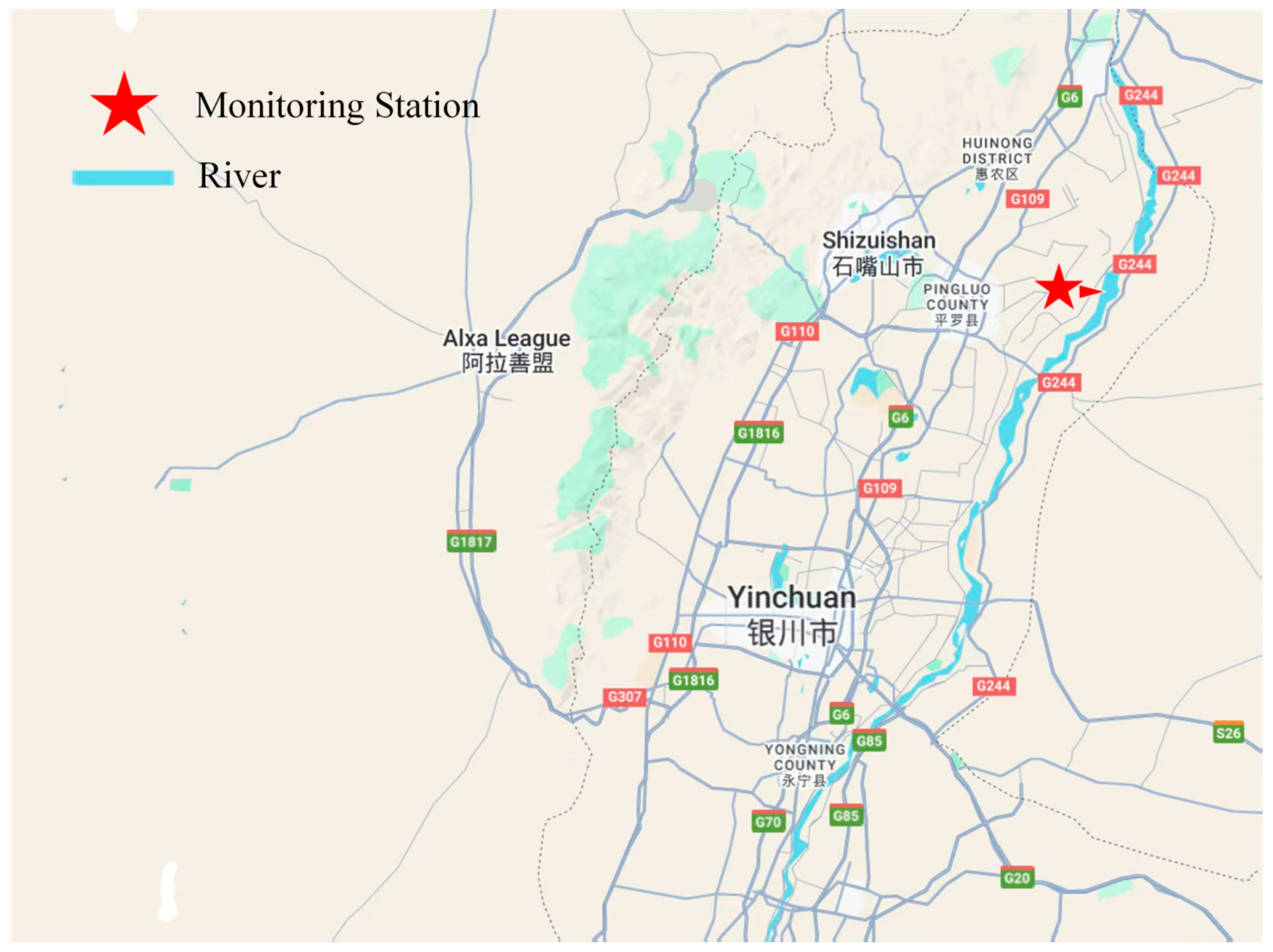
(3) The validation based on the measured data from Shizuishan hydrological monitoring site in the Yellow River basin shows that the fusion model leverages the advantages of two-way feature extraction and attention weighting, and it outperforms traditional methods in terms of prediction accuracy and stability, which provides an effective solution for hydrological forecasting.
2. AT-BiLSTM for Water Flow Forecasting
2.1. The Proposed AT-BiLSTM Model
Bi-LSTM can capture the causal chain and feedback effects of hydrological systems synchronously through forward and reverse time-series modeling, and its bidirectional information flow architecture can not only parse the forward transmission process of precipitation-runoff but also retrace the temporal and spatial hysteresis characteristics of flood wave propagation in the reverse direction. However, the hidden state vectors of traditional LSTM are prone to feature compression effects in time-series iterations, leading to the weakening of key hydrological events (e.g., abrupt signals during the flood peak formation period) in long-term dependent modeling. To this end, the attention mechanism reconfigures the feature space through dynamic weight allocation—its bionic design mimics the selective focusing property of human cognition—to autonomously identify key time periods in the hydrological sequence with predictive value. The coupling innovation between the two is reflected in the fact that Bi-LSTM provides a bidirectional temporal base model, while the attention layer constructs a “global-local” feature interaction paradigm through the synergistic effect of feature enhancement and noise suppression.
In this study, an innovative AT-BiLSTM was proposed for river water flow time-series prediction. As depicted in
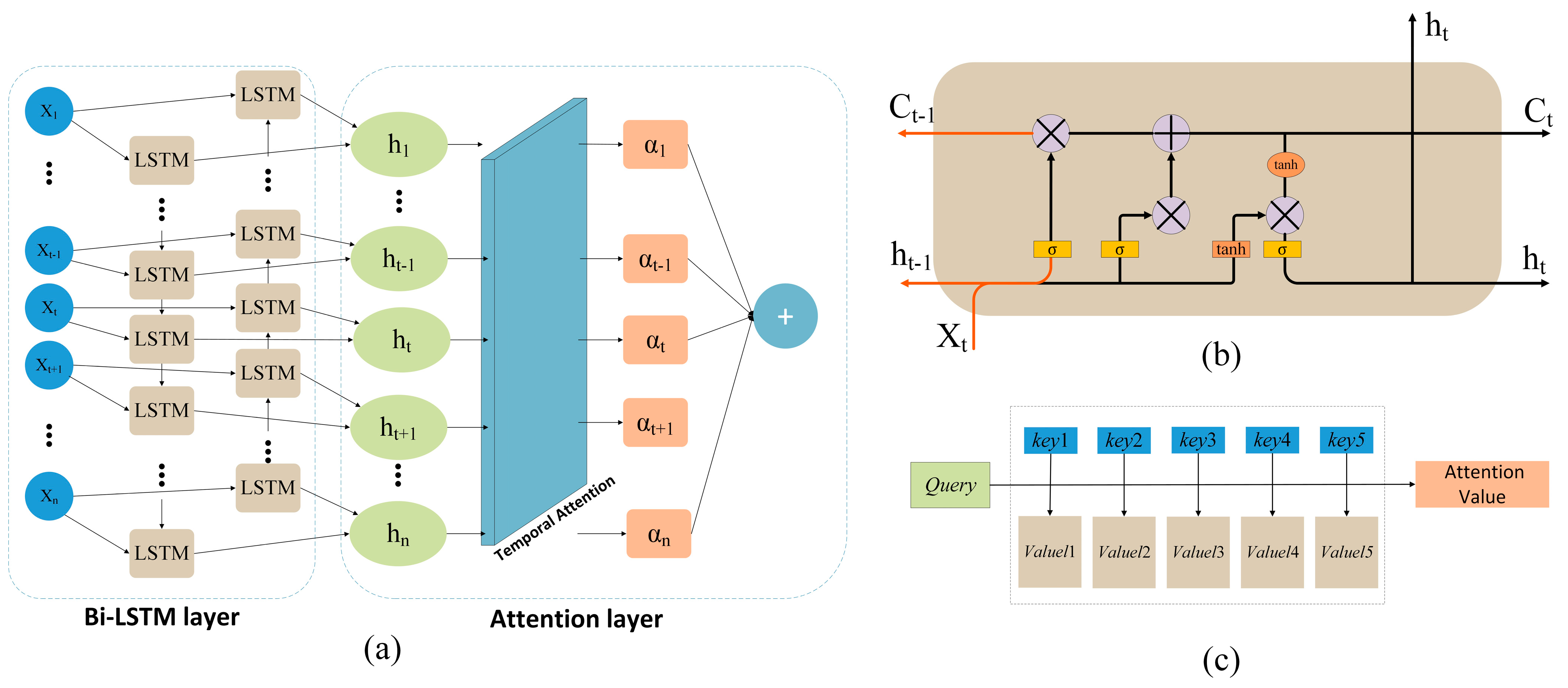
Figure 1, the model architecture consists of a bidirectional time-series feature extraction module and a dynamic attention optimization module (part of the model’s code can be found in
Appendix A), and its core innovation is to break through the bottleneck of traditional hydrological prediction models in the characterization of complex spatiotemporal correlations through the synergistic mechanism of the bidirectional information flow and the feature weights adaption. Specifically, the Bi-LSTM layer adopts a two-way stacked structure (forward LSTM and reverse LSTM), which analyzes the forward physical evolution of the runoff formation process (e.g., precipitation infiltration–surface runoff response) and the reverse system feedback characteristics (e.g., hysteresis effect of flood wave propagation), and dynamically integrates the two-way hidden states through the gating mechanism to form the feature expression with the spatiotemporal coupling effect. The temporal attention layer introduces a learnable weight assignment matrix on this infrastructure, and its bionic design simulates the decision-making cognitive process of hydrologists—analyzing historical sequences based on a sliding time window, identifying the key time periods affecting the prediction target autonomously, and realizing the dynamic reconstruction of the feature space through the Softmax function. The principles and implementation of the functional modules of bidirectional layer and attention layer are described in detail in
Section 2.2 and
Section 2.3.
2.2. Bi-LSTM Layer
LSTM is composed of the input layer, hidden layer and output layer, and the core of the network is the hidden layer with memory function. It includes input gate, output gate, forgetting gate and memory unit block. Xt denotes the input data at the current moment, Ct−1 denotes the cell state at the previous moment, ht−1 denotes the output at the previous moment (or the hidden state at the previous moment), Ct denotes the state of the current memory unit, ht represents the output value at the moment t (or the current hidden state), ft represents the forgetting gate (it represents the hidden state), it determines what information needs to be updated, ht represents the output value at the moment t (or the current hidden state), and Ot denotes the output gate. The input gate and the output gate are control gates, where the input gate decides the amount of information to be transmitted to the memory cell, thus realizing the updating of the cell state Ct. The output gate decides how much information in the memory cell will be transmitted to the current output. The forgetting gate controls the memory cell and is used to determine the memorization and forgetting of the memory cell.
Bi-LSTM is an extended structure of traditional LSTM, which refines its ability to construct bidirectional dependencies of time series by integrating forward and reverse time-series processing capabilities. Its core innovation is to construct a bidirectional information flow mechanism to synchronize and capture the causal transmission and feedback effects of the water flow forecasting (as shown in
Figure 1b). Forward LSTM and reverse LSTM are employed to obtain the hidden layer states of two time series that are opposite to one another. These time series are then connected to obtain the same output, and other procedures are similar to those in the LSTM training process. The forward and backward information of the current input sequence can be obtained using the forward LSTM and re-verse LSTM, respectively. The reverse LSTM adopts a reverse time-series input, whose mathematical expression is symmetrical to the forward LSTM, as shown in Equations (1)–(5) [
24,
25].
where
is the inverse LSTM weight matrix,
is the bias term,
σ is the Sigmoid activation function, ⊙ is the Hadamard multiplication (element-by-element), [·; ·] is the vector splicing operation,
Ct+1 denotes the cell state at the next moment, and
ht+1 denotes the output value at the next moment
t + 1.
2.3. Attention Layer
The attention layer constructed in this study adopts the Key-Value-Query (KVQ) paradigm to realize dynamic reconstruction of the feature space (in
Figure 1c), whose core function is to strengthen the contribution of key hydrological features to the prediction target through a learnable weight assignment mechanism. Specifically, the hidden state sequences (
) output from the Bi-LSTM are utilized as the input source, where the feature vectors
at each time step contain both forward and backward time-series information. The process of calculating the attentional weights is as follows [
25,
26].
- (1)
Feature mapping: to generate query vectors Qt, key vectors Kt and value vectors Vt by linear transformation (in Equation (6)),
where
WQ,
WK, and
WV are the matrix of trainable parameters.
- (2)
Similarity measure: the scaled dot product was utilized to calculate the correlation between the query vector and the key vectors at each time step (in Equation (7)),
- (3)
Weight normalization: generating the attention distribution by Softmax function (in Equation (8)),
- (4)
Context vector synthesis: a sequence of weighted aggregated value vectors is obtained by Equation (9).
The design inherits the core idea of Transformer, but adapts it for hydrological timing characteristics—reducing computational complexity by constraining the length of the time window, while retaining the ability to model long-range dependencies. This makes the hydrological modeling properties physically interpretable and dynamically feature selectable.
2.4. Training Process of the Proposed Model
In this investigation, the data is divided into a training set and a test set. The prediction model is first trained on the training set and then the test set is selected to evaluate the performance. The specific training process is as follows:
Step 1. Data input: the sample data are imported into the model input vector.
Step 2. Feature extraction: to handle the input vector through Bi-LSTM hidden layer.
Step 3. Weight calculation: based on the hidden state and cell state of Bi-LSTM, calculating the weights of each moment using the attention mechanism.
Step 4. Output: acquiring the final prediction outcome after handling by the fully connected layer.
Once the model is trained, it forms an end-to-end prediction system, which realizes the whole process of automated inference from data input to the predicted value of water flow. Through the synergy of bidirectional LSTM and attention mechanism, the architecture can accomplish dynamic extraction and weight assignment of spatiotemporal features without manual feature engineering.
4. Results and Analysis
For this experiment, the water flow data from the upstream portion of the Yellow River Basin were chosen. The data volume was 1096 sets, and the data recording period was from 1 January 2018 to 31 December 2020. Additionally, we separated each dataset into training and testing sets in accordance with 9.5:0.5 in order to meet the needs of the experiment. The following settings were used to construct an experimental environment in this study using the deep learning framework PyTorch: Python 3.6.9, Win11 64-bit operating system, Intel i5-11320H 3.19 GHz CPU, and 16G RAM.
4.1. Benchmark Models
The following five models were compared to the proposed AT-BiLSTM; each is displayed below:
EXPS: A popular technique in production forecasting for short- and medium-term economic trend forecasting is exponential smoothing, or EXPS.
ARIMA: It consists of auto regressive (AR), integrated (I) and moving average (MA) components. It predicts future data through autoregression and moving average of past data, and it is widely used for time-series forecasting in economics, finance, meteorology, and other fields.
RNN: It is a class of neural networks adopted to process sequence data. Unlike feed-forward neural networks, RNNs have a recurrent structure that captures temporal dependencies in sequence data.
LSTM: It is a deep learning model for processing data sequences and is a common variation of RNN. Three gates (input, forget, and output gates) and a cell state are introduced by LSTM in contrast to typical RNN. These features enable LSTM to manage long-term dependencies in sequences more effectively.
Bi-LSTM: It combines forward LSTM and reverse LSTM for prediction.
4.2. Optimization and Selection of Experimental Parameters
In this study, the Holt-Winters exponential smoothing model was used for EXPS to achieve automatic seasonal detection of river flow data. In time-series analysis, the ARIMA model is a widely used forecasting model. To determine the optimal order of the model (where p is the order of the autoregressive term, d is the number of difference steps, and q is the order of the moving average term), in information criteria, Akaike Information Criterion (AIC) and Bayesian Information Criterion (BIC) usually are chosen. In hydrologic forecasting studies, AIC and BIC are statistical scales for model selection to balance the conflict between model complexity and goodness-of-fit. For example, AIC not only improves the model fit (great likelihood) but also introduces a penalty term so that the model parameters are as few as possible, which helps to reduce the possibility of overfitting. The penalty term of BIC is larger than that of AIC, and when the number of samples is too large, it effectively prevents excessive model complexity caused by excessive model precision. The smaller the values of AIC and BIC are, the better the model fits. While higher-order ARMA models enhance their ability to describe the sample data, they also increase the number of parameters, which can lead to overfitting.
Table 1 shows a comparison of the performance of the automated methods for selecting the best ARIMA parameters. From
Table 1, it can be seen that the best model parameters of ARIMA are (0,1,1) for water flow forecasting.
Similarly, we employed a systematic hyperparameter calibration process to optimize the key configurations of the model structure through validation sets. The core hyperparameters, including the learning rate, number of training rounds (epochs), and hidden layer dimension, were searched globally in a space using a Bayesian optimization framework (Optuna framework). The optimization objective focused on maximizing the model’s ability to generalize hydrologic time-series features and its prediction accuracy. The final parameter selection was the result of optimization considering multiple objectives, such as smaller MSE and larger R2. This balanced prediction accuracy and computational efficiency and ensured that the model was reliable and could be used in hydrological scenarios.
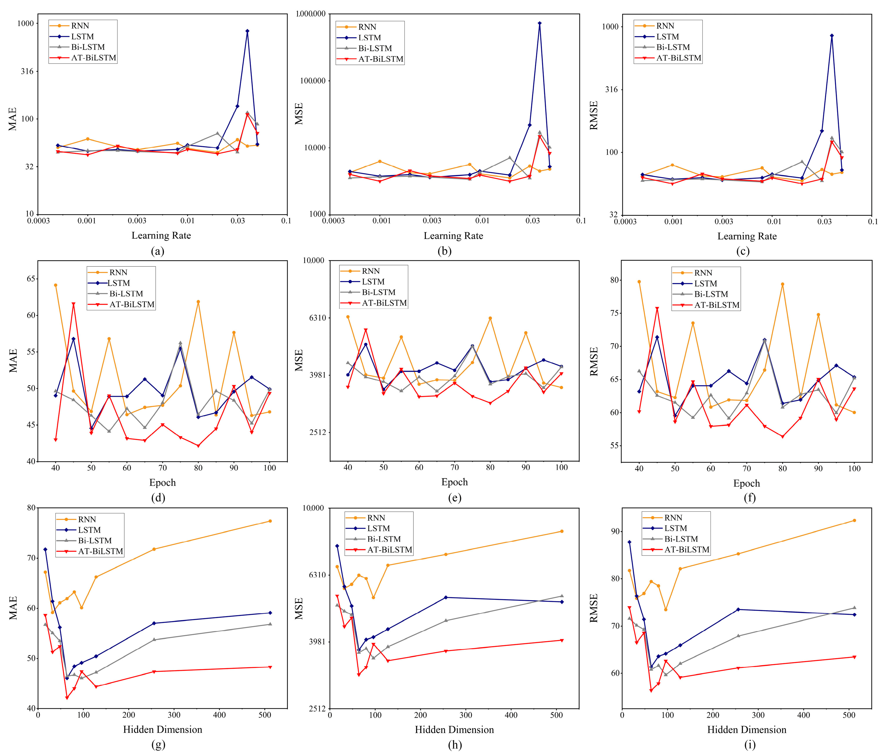
Figure 3 illustrates the relationship between the three key evaluation metrics (MAE, MSE, and RMSE) and the key hyperparameters (learning rate, ephemeral elements, and hidden dimension) for the four core sequence models (RNN, LSTM, Bi-LSTM, and AT-BiLSTM) on the test set. The visualized subplots showed a more consistent trend (as shown in
Figure 3).
Figure 3a–c show the nonlinear effect of learning rate on model performance. Moderately increasing the learning rate (0.0005–0.01 range) effectively reduced the prediction error, but too high a value (>0.03) destabilized the training process and led to a sharp decrease in model performance. The attention-enhanced AT BiLSTM showed more desirable robustness to learning rate fluctuations (MSE nearly 10% lower than the baseline RNN). The training iteration process in
Figure 3d–f illustrates that the error metric initially decreased over 40–80 epoch and then stabilized as the number of repetitions decreased. Notably, the bidirectional architecture (Bi-LSTM/AT-BiLSTM) achieved more optimal performance than the unidirectional architecture. However, prolonged training beyond 90 epochs may lead to mild overfitting, especially in the complex AT-BiLSTM, where the validity error (MAE) increased by 20%. Hidden layer dimensionality studies (
Figure 3g–i) identified critical capacity thresholds: hidden dimensions < 32 limit edmodeling capabilities (with higher MAE), while hidden dimensions > 128 led to over-parameterization. In the optimal configuration, the AT-BiLSTM with 64 hidden dimensions had a minimum MAE of 42.19, outperforming the smaller (16 hidden dimensions: 58.61) and larger (512 hidden dimension: 48.32) variants.
4.3. Model Performance Analysis
To validate the effectiveness of the proposed model in river water flow forecasting, we conducted comparative experiments with two categories of baseline models: classical statistical approaches (EXPS and ARIMA) and mainstream deep learning architectures (RNN, LSTM, and Bi-LSTM). The proposed AT-BiLSTM distinguished itself from conventional LSTM/Bi-LSTM through its integration of bidirectional temporal modeling and attention mechanisms, while retaining their core structural framework. All baseline models were configured with hyperparameters optimized for their peak performance.
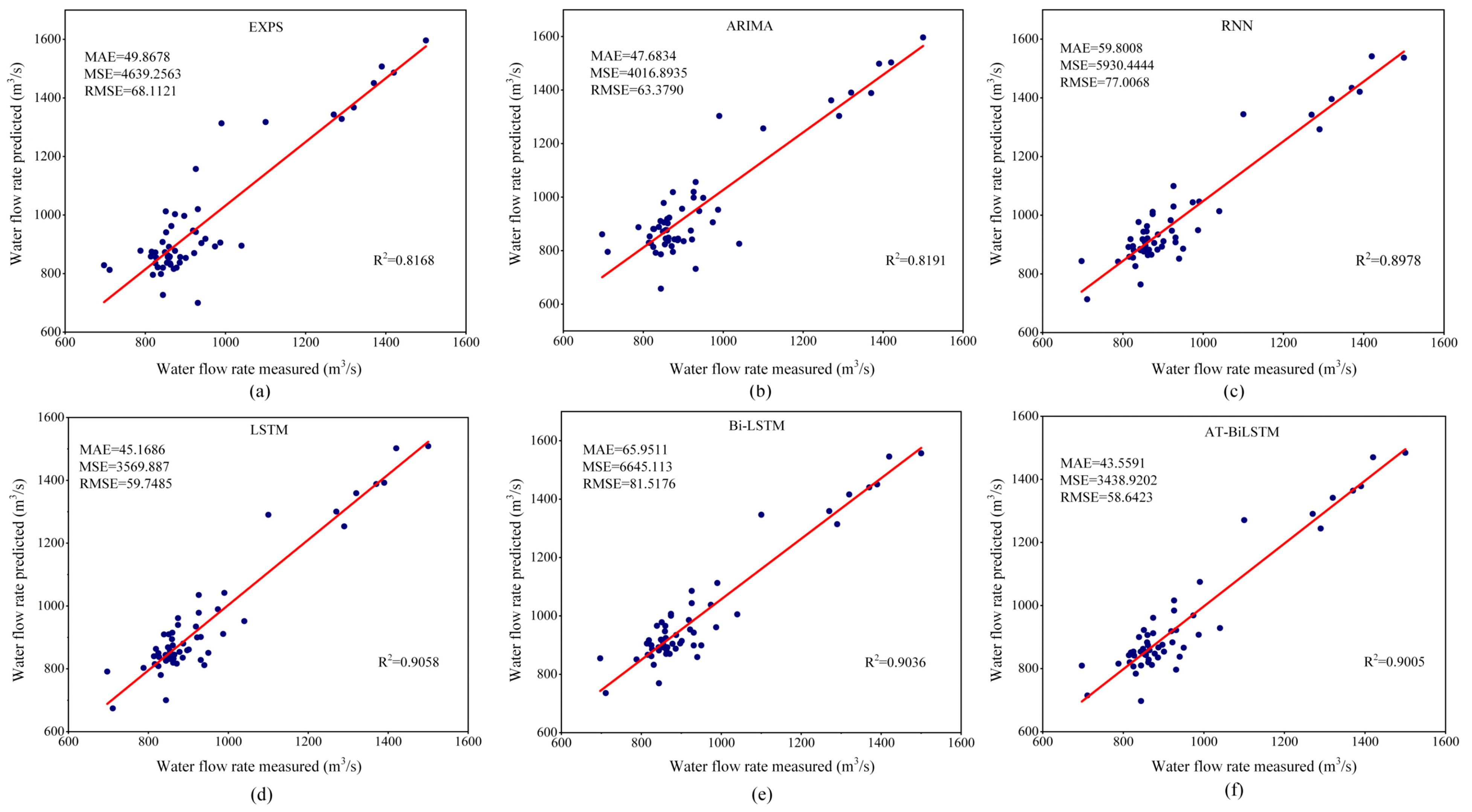
A comparison of the prediction performance of the five baseline models and the proposed AT-BiLSTM model on the dataset is depicted in
Figure 4. The MAE, MSE, and RMSE results are shown in the upper left corner of each subplot, while the R
2 scores are shown in the upper right corner. For all river flow forecasting methods, the ideal state model with predicted values (denoted as discrete points) clustered around the diagonal and aligned with the observed values. The results indicate that the proposed AT-BiLSTM had a better overall performance in water flow forecasting compared to the EXPS, ARIMA, RNN, LSTM, and Bi-LSTM baselines. Among these six methods, the classical conventional models did not perform as well as the mainstream deep learning methods, e.g., EXPS had the worst R
2 (0.8168). Notably, all three models—LSTM, Bi-LSTM, and AT-BiLSTM—achieved R
2 values above 0.9, proving their very good data fitting ability. Among the four deep learning models, the RNN ranked the lowest (MAE = 59.80), trailing behind the LSTM, Bi-LSTM, and AT-BiLSTM. It is noteworthy to note that the integration of the mechanism reduced the MAE, MSE, and RMSE in the Bi-LSTM framework. This improvement stemmed from the ability of the attention layer to dynamically weight the input features over time steps. Similarly, replacing LSTM with Bi-LSTM improved temporal pattern capture by augmenting the error metric with bidirectional learning of the hydrological time series during pre-training. By synergistically combining Bi-LSTM and the attention mechanism within the standard LSTM architecture, the proposed model significantly reduced the MAE, MSE, and RMSE on the Shizuishan Yellow River dataset by 27.16%, 42.01%, and 23.85%, respectively, compared to the baseline RNN.
To further validate the robustness of the proposed AT-BiLSTM model in river water flow forecasting, we performed several training iterations and test validations on the entire dataset.
Table 2 lists the performance of the model in four independent retraining trials for the water flow forecasting task. The results show that the AT-BiLSTM water flow prediction model achieved excellent overall performance in all metrics (MAE, MSE, RMSE, and R
2) compared to the five benchmark models. Notably, the fluctuation ranges of the MAE and RMSE values of AT-BiLSTM were significantly reduced compared with those of RNN, LSTM and Bi-LSTM, confirming its better robustness. For example, the MAE values of AT-BiLSTM ranged from 42.63 to 44.76 (with a variation rate of 4.8%) over four trials, whereas the MAE values of LSTM ranged from 44.14 to 59.78 (with a variation rate of 26.2%), which showed greater volatility.
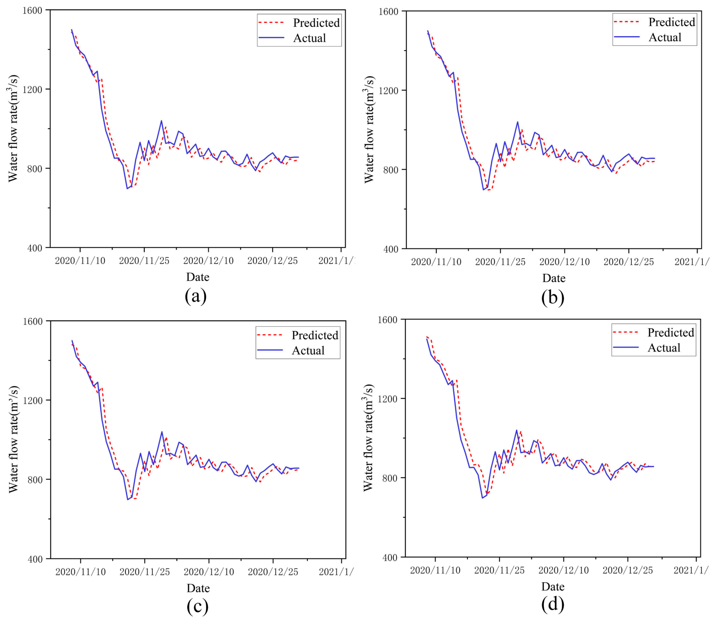
To display the data in
Table 2 more intuitively, we expressed the prediction results of the AT-BiLSTM model in four subfigures separately.
Figure 5 shows the prediction trajectories of four independently trained AT-BiLSTM models, where the blue curves indicate the actual measurements and the red dashed lines indicate the model predictions. The results show that the agreement between predicted and observed values was very high in all four subplots, and the proposed AT-BiLSTM consistently achieved the desired prediction performance in all training variants.
4.4. Ablation Study for AT-BiLSTM
The ablation experiment is a commonly utilized experimental design method, especially in the fields of machine learning. The main purpose is to analyze the impact of gradually removing or modifying certain parts of the model on the overall model performance. In this subsection, we verify the improvement effect of the proposed Bi-LSTM layer and attention mechanism on the standard LSTM through ablation experiments.
Table 3 lists the parameter details for standard and various variants of LSTM models in the ablation experiments.
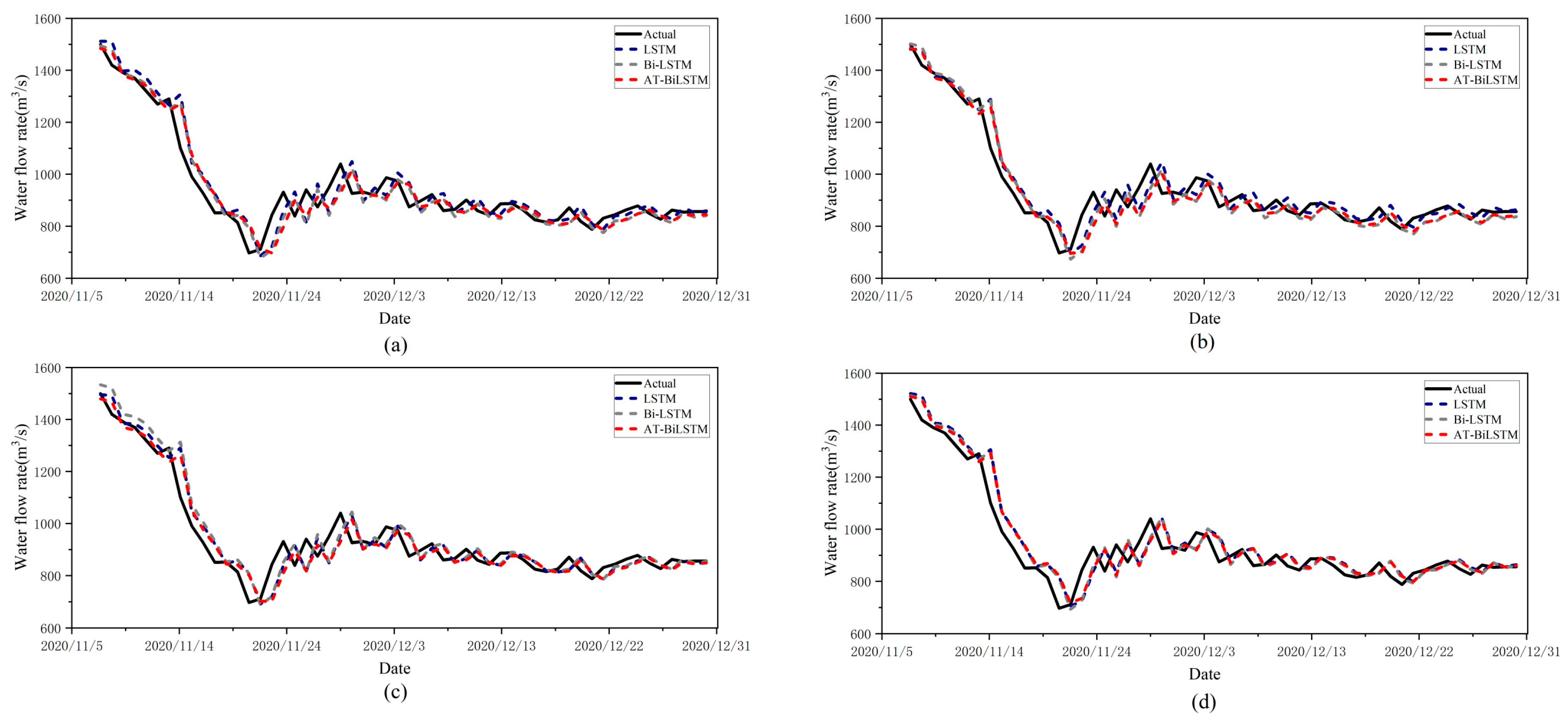
To evaluate the predictive performance and robustness of three LSTM variants, we conducted ablation studies by calculating the relative error fluctuation rates across four independently trained models.
Figure 6 and
Figure 7 systematically present the comparative model analysis and error distributions from this ablation framework. The closely aligned trajectories across all four subplots in
Figure 6 demonstrate strong architectural stability during repeated training trials. The visual analysis of operational details (e.g.,
Figure 6a magnification) reveals that the proposed AT-BiLSTM with attention mechanisms outperformed baseline LSTM/Bi-LSTM counterparts in both trend alignment and peak–valley feature capture. The relative error distribution for each model is shown in
Figure 7. Overall, it can be concluded that the attention mechanism enhanced the prediction accuracy of the majority of sharp points and lowered the error percentage of the regular Bi-LSTM and LSTM models.
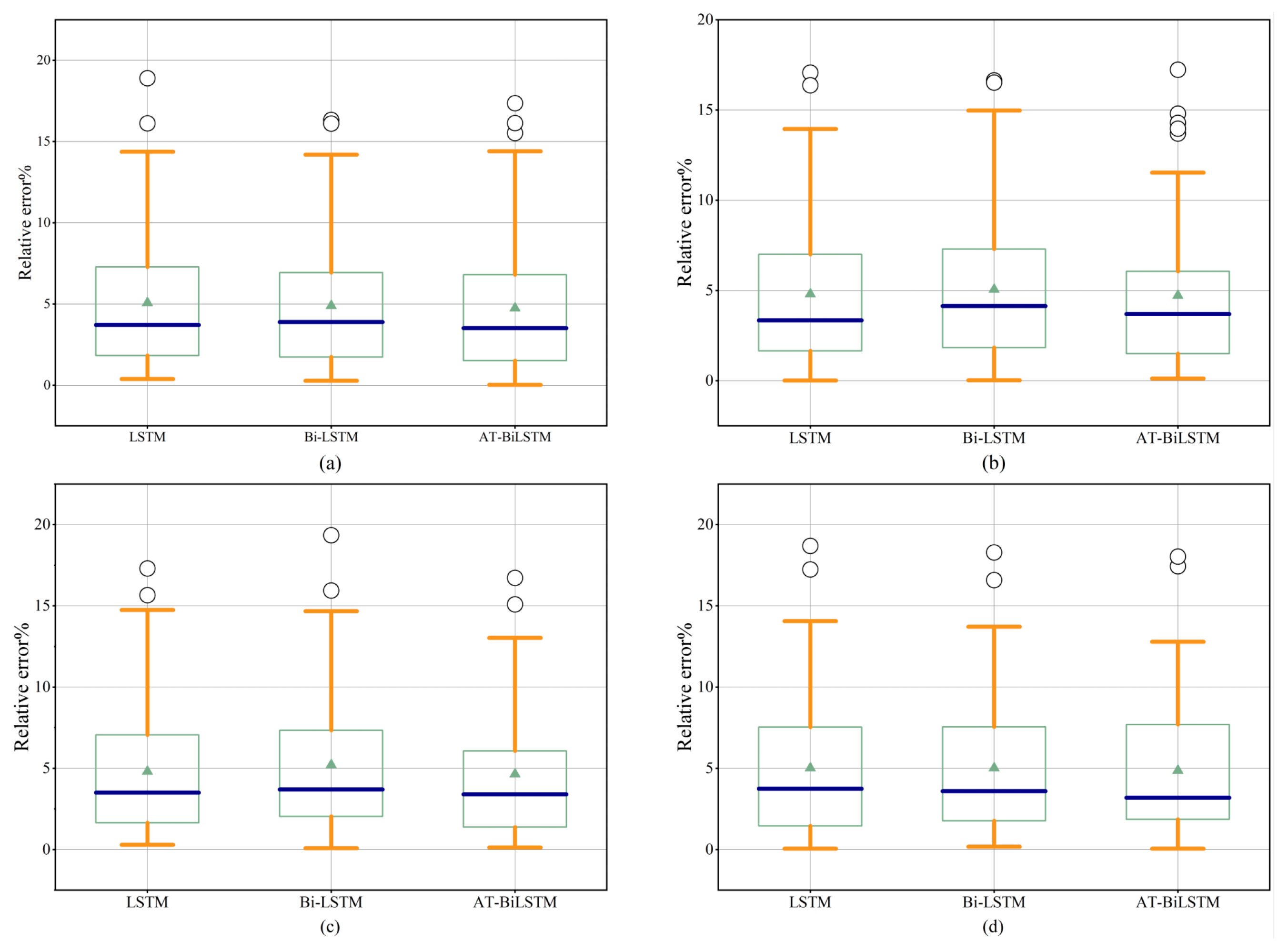
Figure 8 displays boxplots of percentage relative errors for three models across four tests. From
Figure 8a,c,d, it can be observed that the LSTM model exhibited larger relative errors in its outliers (represented by circles), indicating significant deviation from true values and pronounced error fluctuations in most predictions. In contrast, the Bi-LSTM model demonstrated moderate relative errors, while the AT-BiLSTM model showed a relatively higher number of outliers in
Figure 8b but maintained lower outlier error magnitudes in other subfigures, reflecting superior error control and prediction stability in most scenarios. Further analysis of the error ranges (represented by the whiskers of the boxplots) reveals that the LSTM model had the widest error distribution in
Figure 8b–d, suggesting high sample-to-sample variability and poor stability. The Bi-LSTM model exhibited relatively narrower error ranges, indicating moderate robustness. The AT-BiLSTM model displayed the most compact error ranges in all cases except
Figure 8a, demonstrating concentrated error distributions with minimal dispersion. The median lines (dark horizontal bars) across all subfigures show significant inter-model differences. The AT-BiLSTM achievesdthe lowest median errors under all experimental configurations, confirming its consistent high-precision performance across four tests. In summary, comprehensive evaluation based on outlier errors, median errors, and error ranges demonstrates that the AT-BiLSTM model significantly outperformed conventional LSTM and Bi-LSTM models in prediction accuracy, stability, and noise resistance.
4.5. Effect of Attention Mechanisms
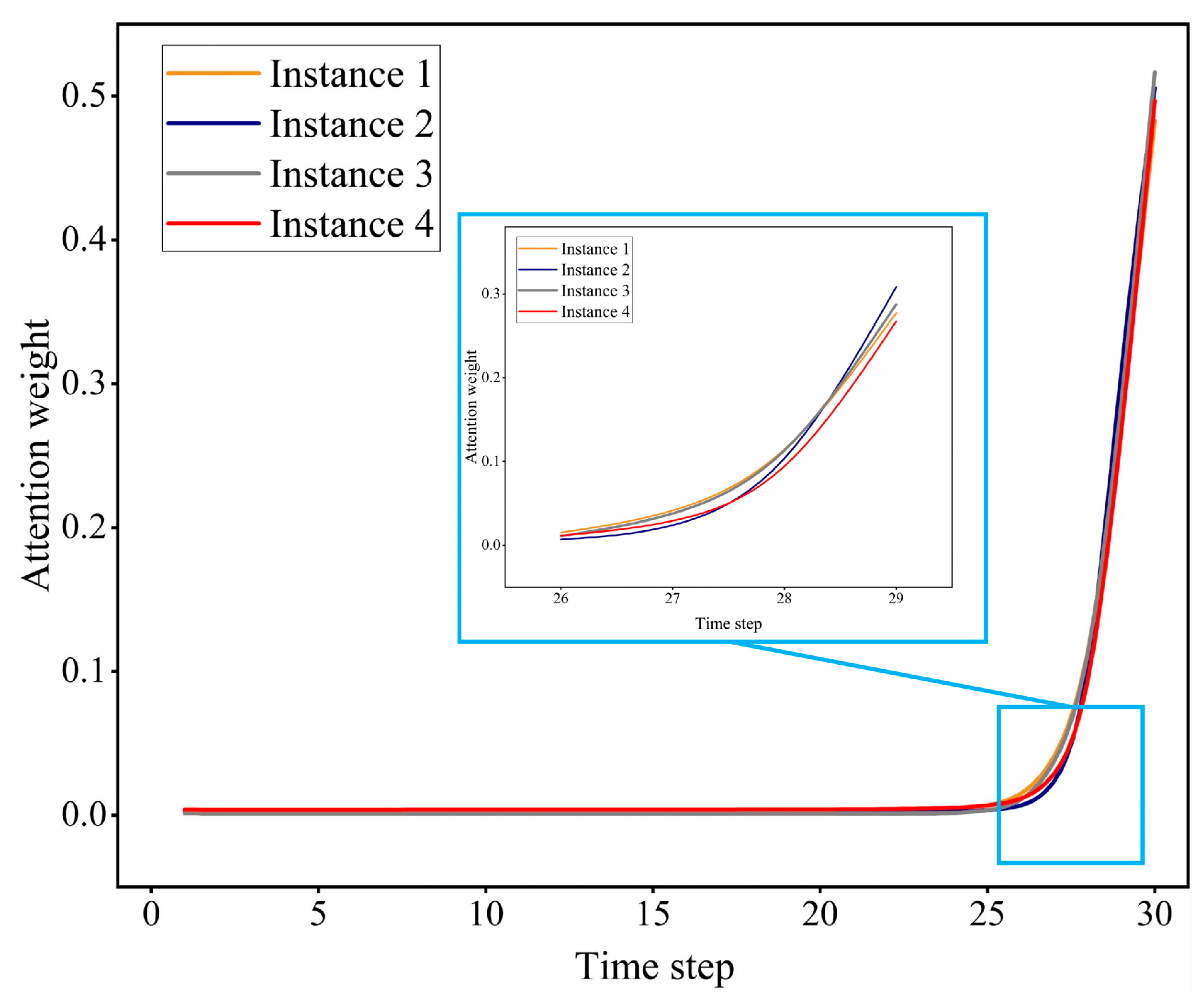
This subsection focuses on the temporal attention dynamics of the AT-BiLSTM model, employing visualization techniques to demonstrate its attention allocation patterns in different time steps.
Figure 9 illustrates the evolution of the attentional weights of the input sequences in four independent training instances of AT-BiLSTM, where the
x-axis denotes the prediction time step and the
y-axis quantifies the values of the attentional weights. The analysis shows that the attentional weights exhibited a dynamic adjustment as the prediction time progressed, as manifested by the gradual strengthening of their weights within the temporal attention tilt. This mechanism can focus the attention differentially on key historical points in the time series, thus improving the prediction performance of the model.
4.6. Effect of Dynamic Backtracking Window Size
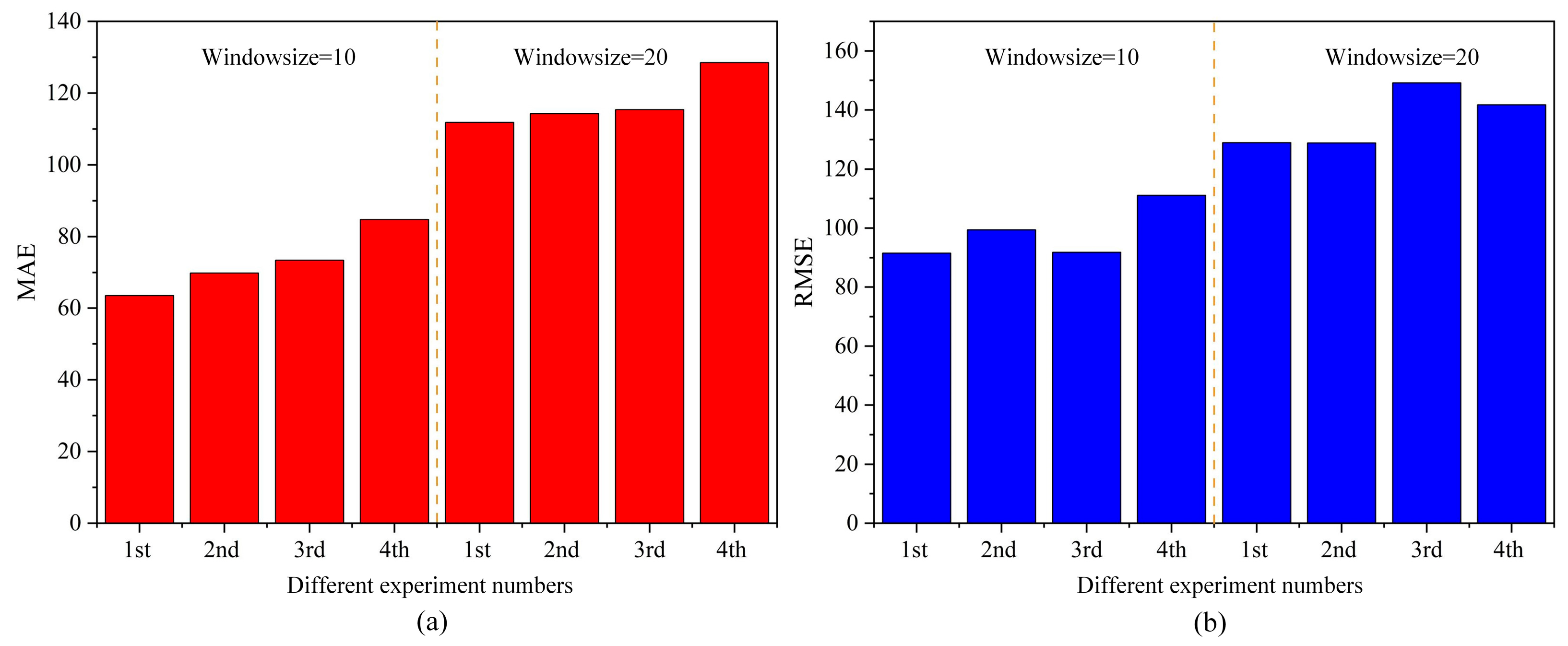
Compared with the existing models, one of the innovations of the proposed AT-BiLSTM model of river water flow is that it can dynamically adjust the time retrospective window according to the basin characteristics (dry/flood season) by combining the adaptive attention mechanism. For the normal or dry water period, the period of the time retracement window in the AT-BiLSTM model proposed in this paper is long, generally in the range of 20~30 days. However, we found that for flood season forecasting, a retrospective window period that is too long will affect the prediction performance of the model.
Figure 10 shows the comparison of MSE and RMSE of the model under different retrospective window periods during the flood season.
Hydrological series data are different from weather and stock price time series in that it has more obvious seasonality. Therefore, they can automatically select different time retracement window parameters according to the basin characteristics (dry season/flood season/normal), so that the model could realize the adaptive attention mechanism and improve its own performance.
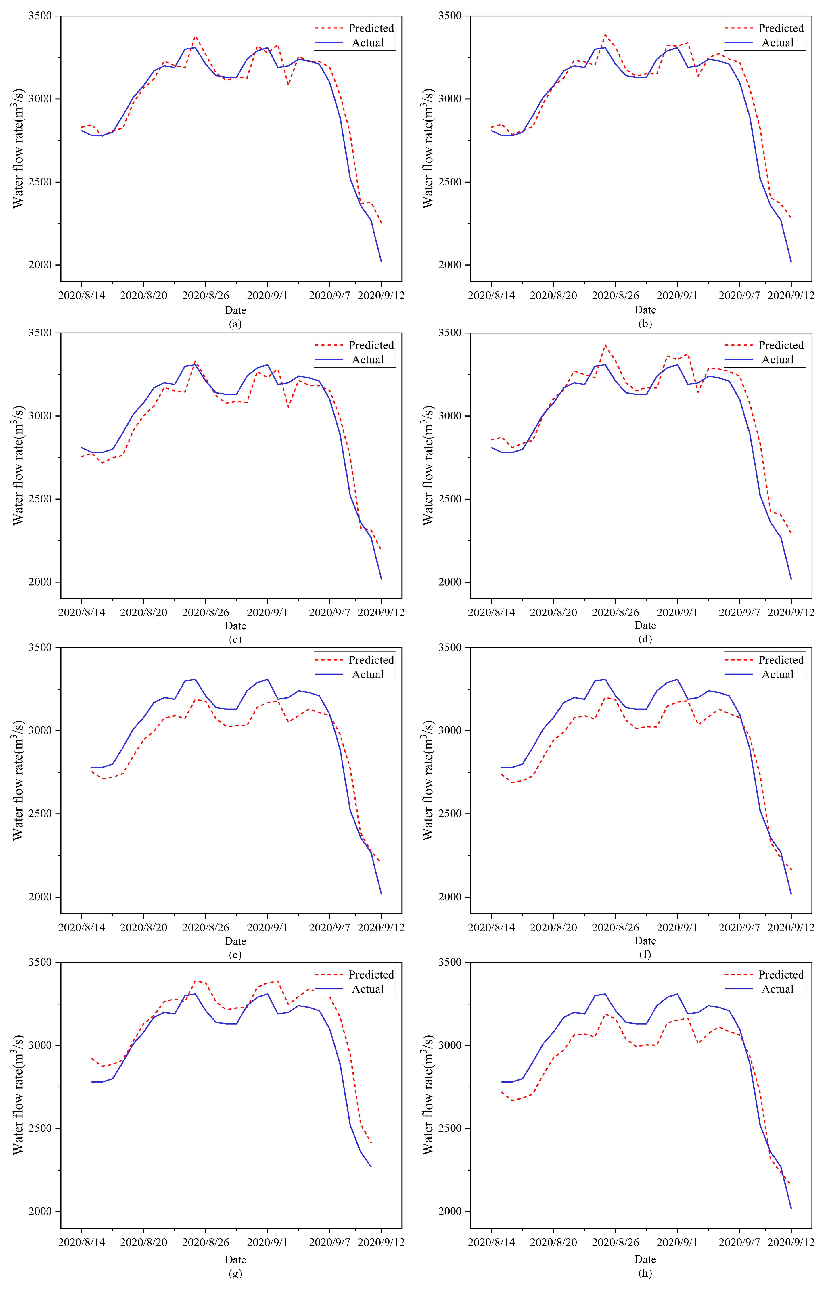
Figure 11 shows the comparison of the predicted and actual values of the model for four independent training sessions under different time retracement window parameters during the flood season. We found that the prediction performance of AT-BiLSTM could be improved by dynamically changing the time retracement window parameters (windowsize). This allows its prediction performance to be improved even during flood season to meet the requirements of its application scenarios.
4.7. Performance Comparison of 1–7-Day Forecasts
The 1–7-day river flow forecast is crucial for flood and drought warning as well as water resource management. Traditional physical models are difficult to effectively couple multi-source driving factors (precipitation, snowmelt, reservoir regulation) with nonlinear runoff evolution relationships, while data-driven methods have limitations in interpretability. Deep learning techniques such as RNN, LSTM, and their variants have driven the development of this field through their ability to extract temporal features: RNN has initially achieved runoff sequence memory modeling, but is limited by the problem of vanishing gradients; LSTM extends the effective memory through gating mechanism, improves the forecasting time span, and enhances the model’s forecasting ability; Bi-LSTM further introduces bidirectional temporal processing to enhance the analysis of upstream and downstream hydraulic interactions. In addition, the application of attention mechanisms such as AT-BiLSTM further enhances the performance of LSTM models.
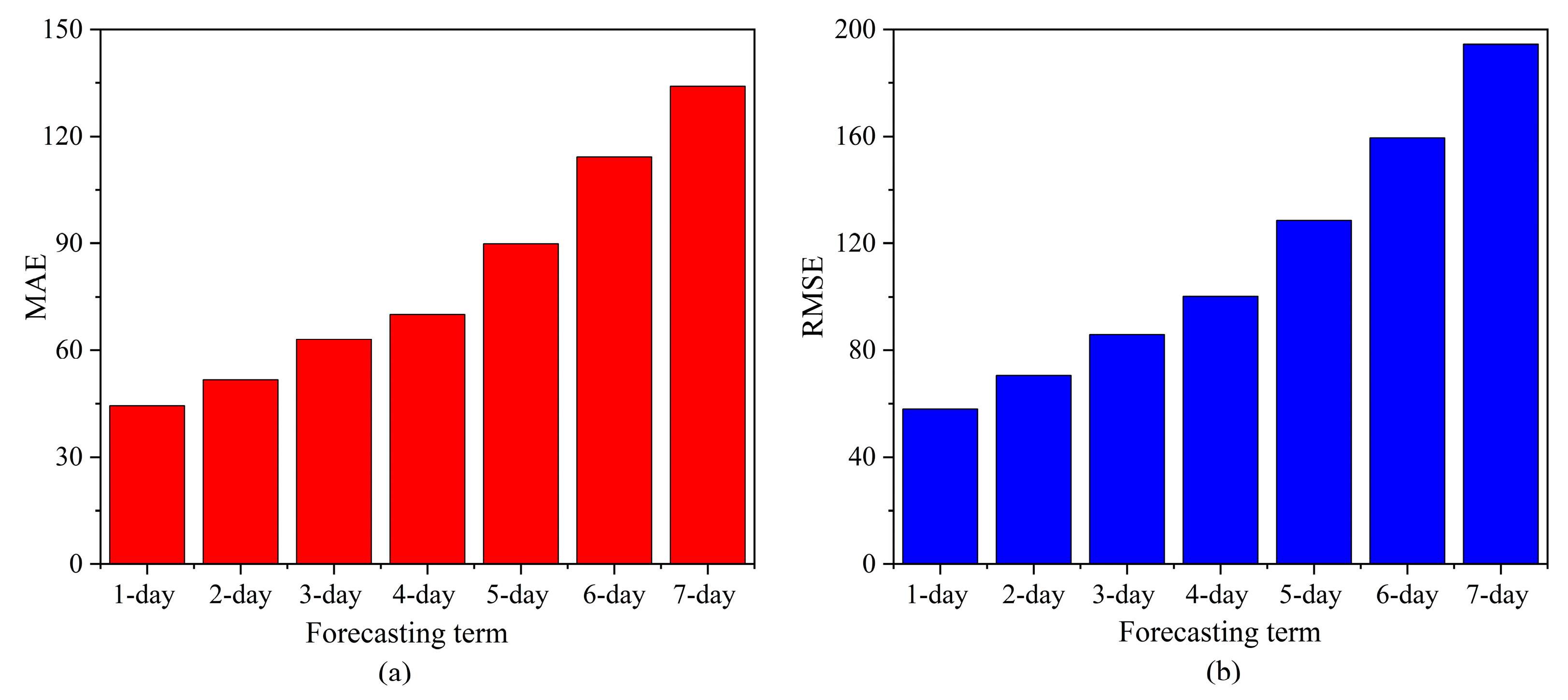
Figure 12 presents a comparative analysis of the AT-BiLSTM model’s performance in 1–7-day river flow forecasting using MAE and RMSE as evaluation metrics. The results indicate a consistent degradation in prediction accuracy as the forecast horizon extends. For short-term forecasts (1–3 days), MAE values were measured at 44.39, 51.61, and 62.99 respectively, demonstrating a gradual error increase within operationally acceptable thresholds. However, a critical performance decline emerged beyond the 5-day horizon, where MAE and RMSE escalated sharply, exceeding practical engineering tolerances. The model exhibited robust utility in 72 h (3-day) forecasts, maintaining an average prediction error margin below 6%—a precision level that aligns with real-world requirements for flood early warning systems and reservoir management. In contrast, the pronounced error amplification in mid- to long-term forecasts (4–7 days) likely reflects challenges in modeling delayed hydrological processes (e.g., groundwater recharge cycles, snowmelt lag effects) and accumulating meteorological uncertainties. These limitations highlight the current applicability boundaries of data-driven approaches in extended hydrological forecasting while affirming their value in short-term operational scenarios.


