Enhanced Early Warning Threshold Setting for Dam Safety Monitoring Based on M-Estimation and Confidence Interval Method

Abstract

Accurate online identification of abnormal sudden change observations is crucial for ensuring data reliability and has been a key challenge in dam safety monitoring. Traditional methods, such as those based on the Pauta criterion, often fail to effectively identify anomalies in complex data sequences like step-type and oscillatory-type data, primarily due to unreasonable early warning threshold settings. To address this issue, this paper introduces a novel method for setting early warning thresholds by combining the scale estimator ST based on the location M-estimator with the confidence interval radius D derived from predicted values, thereby constructing the MZ criterion with a threshold of 3ST+D. The proposed model demonstrates strong resistance to outliers and good robustness, effectively improving the accuracy of online anomaly identification for various data sequences. The MZ standard achieves a false alarm and missed detection rate of less than 10% in the monitoring data of the XB hydropower plant, which is a significant improvement in detection accuracy compared to the traditional Pauta standard. Engineering applications have shown that the MZ criterion-based identification method achieves a low misjudgment and omission rate, high recognition accuracy, and is highly reliable for online dam safety monitoring. This method holds significant value for both theoretical research and practical engineering applications.

1. Introduction

Dam safety has become an area of growing concern worldwide. Monitoring data serves as a vital tool for evaluating the operational status of dams and plays a pivotal role in ensuring their safe and efficient operation. In recent years, with the advancement of remote online dam safety monitoring technologies, the volume and diversity of monitoring data have increased rapidly [1,2]. However, accurately identifying anomalies in monitoring data remains a critical challenge that needs to be addressed to enhance the reliability of dam safety monitoring systems. Sudden changes, often referred to as mutations, in monitoring data can arise from various sources, including failures of monitoring instruments, environmental disturbances, and errors inherent in the monitoring process. Additionally, structural responses of a dam to changes in environmental variables such as reservoir water level, rainfall, and earthquakes can also lead to anomalies in monitoring data [3,4]. These anomalies may reflect a deterioration in the structural performance of a dam, making their timely and accurate identification essential for data reliability and the intelligent control of dam operation safety. With the development of remote online dam safety monitoring, diversity and volume of monitoring data increase rapidly. How to optimize anomaly identification models and improve early warning threshold setting methods in order to improve the reliability and accuracy of online anomaly identification is a key problem that deserves to be studied.

Many methods for anomaly identification of dam safety monitoring data have been proposed so far and can be classified into two categories: One is to select only the data of observation points and apply relevant mathematical theories to test abnormal values, such as statistical tests including the 3σ criterion, the Grubbs criterion and the t-test criterion. The other one is to select data of both measuring points and environmental monitoring and to establish functional models according to the physical cause of the responses [3,5]. Then, anomaly identification can be conducted based on the models. This category contains methods like statistical regression models, hybrid models, deterministic models, etc. Researchers have conducted extensive research on methods for anomaly identification in dam safety monitoring data. Fanelli [6] first proposed a statistical regression model in 1955. From then on, statistical model methods based on multiple linear regression [7,8] (such as least squares regression [4], stepwise regression [9] and robust regression [10]), filtering methods [11], neural network methods [12], genetic algorithm methods [13], etc., were introduced successively for model establishing and early warning threshold setting. The accuracy and applicability of anomaly identification were improved constantly.

For historical sequences with outliers, Erdoğan [14] employed the double-weight estimation in M-estimation to identify anomalous values when studying the effect of reservoir water level changes on dams and achieved satisfactory results. Wang et al. [15] proposed a Kalman filtering algorithm-based M-estimator for deformation monitoring in concrete gravity dams. The MZ criterion, short for median-based Z-score criterion, is defined as $\mathrm{MZ}\text{-}\mathrm{score}={\displaystyle \frac{\left|{\mathrm{x}}_{\mathrm{i}}-\mathrm{median}\right|}{1.4826\times \mathrm{MAD}}}$, where “MAD” represents the median absolute deviation. This robust statistical approach minimizes the influence of outliers on threshold determination. The influence of abnormal observations and dynamic disturbance on monitoring data was controlled. Touati and Benaraba [16] proposed a robust inversion method for jointly estimating parameters and variance components from heterogeneous monitoring data. This method can effectively deal with outliers in dam monitoring data and obtain reliable estimations. In 2019, Wei et al. [17] proposed an improved quantile method for anomaly identification. The method showed high accuracy in the recognition of outliers. In general, the mathematical model identification method based on the Pauta criterion is most commonly used in the online identification of abnormal dam safety monitoring data because it can not only reflect the influence of environmental variables in a comprehensive manner but also is easy for calculation and programming without a loss of reliability.

Identification methods based on the Pauta criterion can easily miss anomalies and misjudge normal values in step-type and oscillatory-type data sequences. In this paper, we proposed a setting method of early warning threshold for abnormal data based on the M-estimator and confidence interval. We also analyzed its applicability and sensitivity to outliers. The application suggested that the proposed model exhibited a good effect on anomaly identification. The method can effectively reduce the occurrence rate of misjudgment, omission, poor reliability and validity of early warning, which usually happen in conventional methods, and can significantly improve the accuracy of online anomaly identification.

2. Challenges in Traditional Abnormal Data Recognition Methods

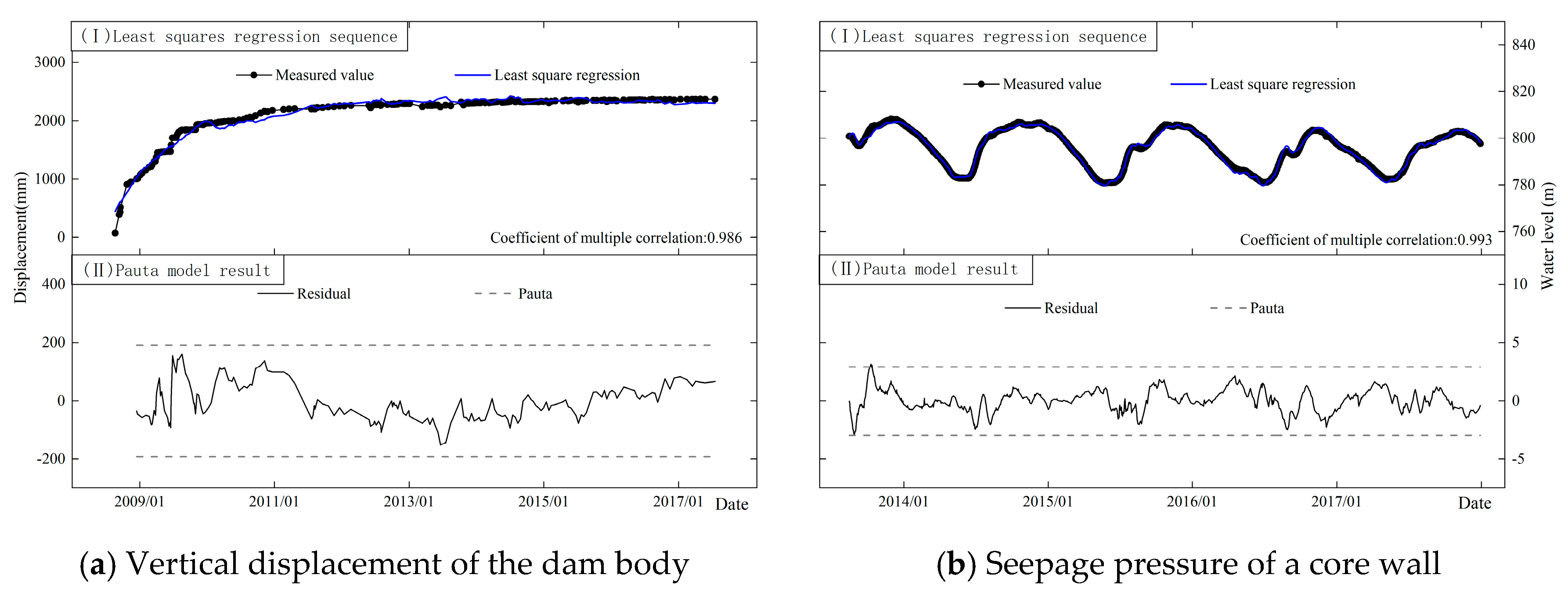
Dam safety monitoring data can obey different rules and can have various types. Property changes in the dam and foundation, equipment-induced short-term abnormal values, significant environmental changes associated with seismicity, construction activities and loadings, etc., would affect patterns of data sequences [18]. The most common patterns observed in monitoring values typically include periodic changes, one-way trend changes, and horizontal linear changes. These patterns can be influenced by various factors such as seasonal variations, long-term structural behavior and stable operational conditions. Anomalies like outliers, small-value data, step-type and oscillatory-type data are also prevalent in monitoring sequences related to dam deformation, seepage and stress. Identifying these anomalies is crucial for maintaining the reliability and accuracy of dam safety assessments. It can be seen in Figure 1 and Figure 2 that these models are ideal for the data sequences with large sample sizes, normal distribution, moderate values and a small number of outliers.

However, they cannot avoid the problems of misjudgments and omissions when dealing with small-value, step-type and oscillatory-type sequences. The reasons are mainly related to the unreasonable setting of the early warning threshold.

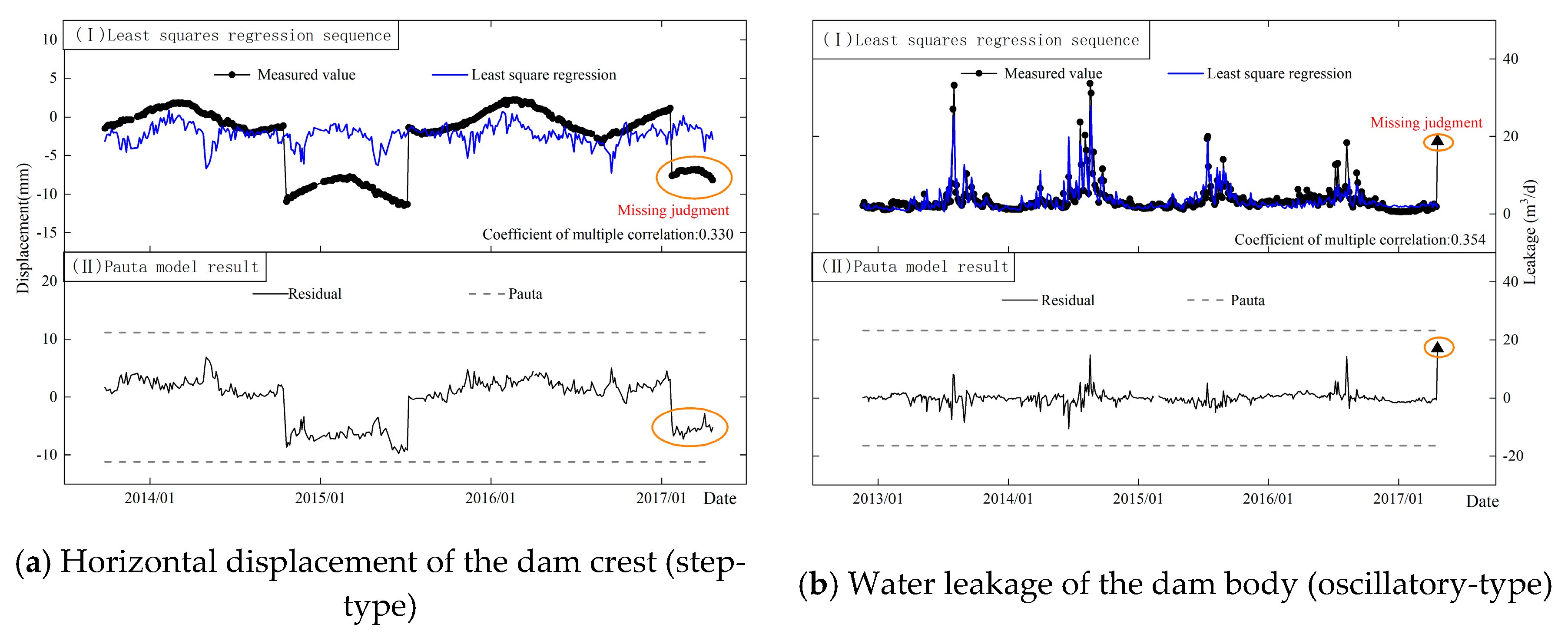
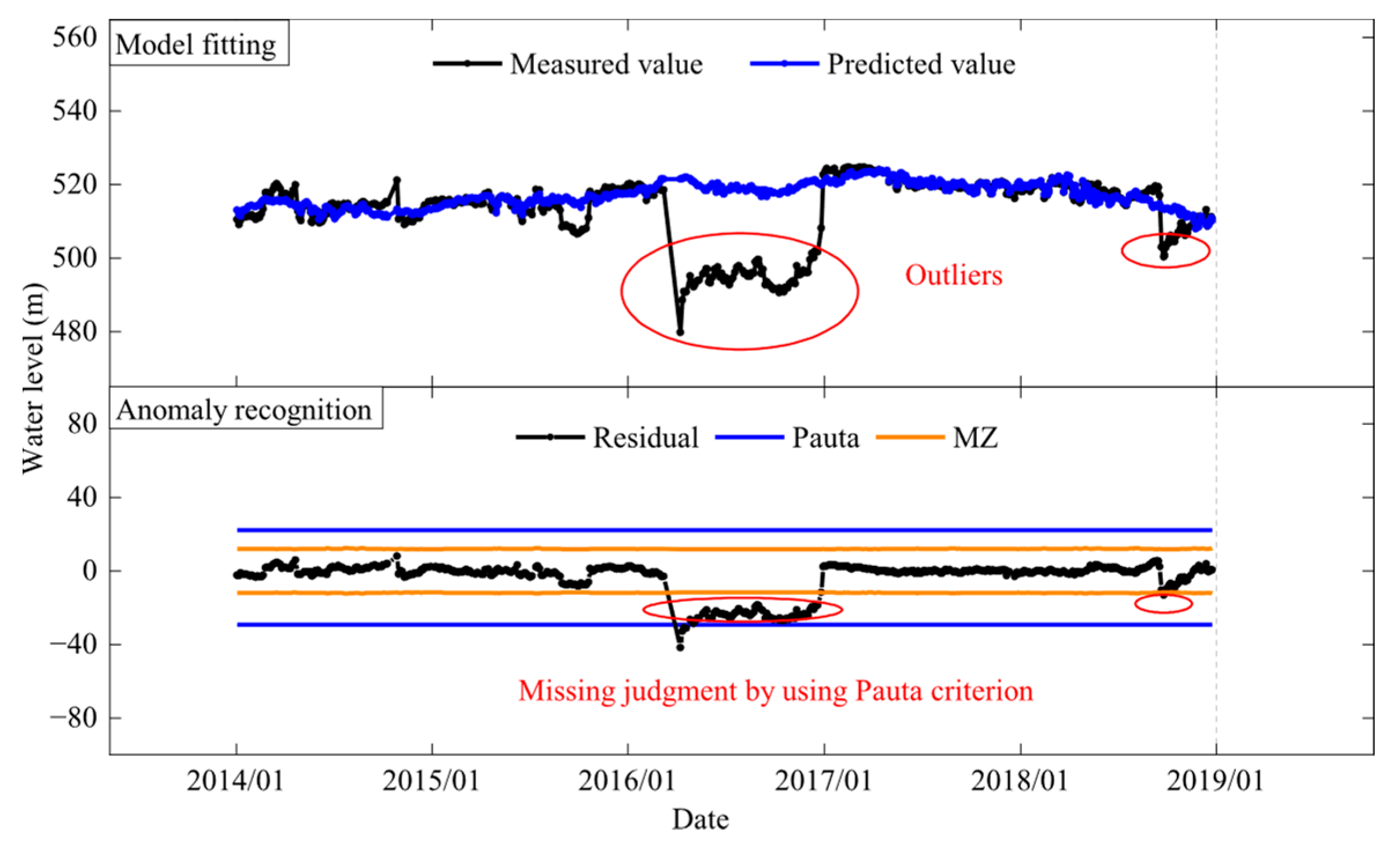
(a) The first issue is the poor interference resistance of statistical estimates and the over-setting of early warning thresholds. There are a large number of outliers in step-type and oscillatory-type data sequences. The regression coefficients solved by the least squares method are still unbiased but are no longer linear unbiased estimates of the minimum variance. That is, a large number of outliers can significantly affect the accuracy of the mathematical model and cause noticeable misfits. Statistical estimates such as means and standard deviations are highly affected by outliers and result in the over-setting of warning thresholds. Then, misjudgments happen, as shown in Figure 3.

(b) Data sequences or residual sequences significantly deviate from the normal distribution assumption of the Pauta criterion. Generally, the anomaly identification methods based on the Pauta criterion are resistant to sequences with a proportion of outliers less than 5%. But the proportion of outliers in step-type and oscillatory-type data sequences is relatively larger. The presence of a large number of outliers would make data sequences and residual sequences deviate significantly from the normal distribution assumption of the Pauta criterion. The Q–Q plot is a graphical method for comparing two distributions. The points in the Q–Q plot will approximately lie on the line y = x if the two distributions being compared are similar. For illustrative purposes, the normality of the residuals of step-type and oscillatory-type data in Figure 3 were tested by a Q–Q plot, and the results were shown in Figure 4. It is obvious that both residual sequences do not satisfy the normal distribution. Thus, it is unreasonable to use the Pauta criterion to set an early warning threshold for non-normally distributed residuals.

(c) Early warning thresholds are set too small for the ignorance of model errors. The regression model is a deterministic relationship inferred from a limited number of response data and environmental data. However, inferences made from the sample to the population can hardly be completely accurate and reliable. Errors always exist in the process of regression. The Pauta criterion considers systematic errors of monitoring instruments and random errors in monitoring operations when setting the early warning thresholds but ignores model errors caused by the estimation of the population based on a limited number of observations.

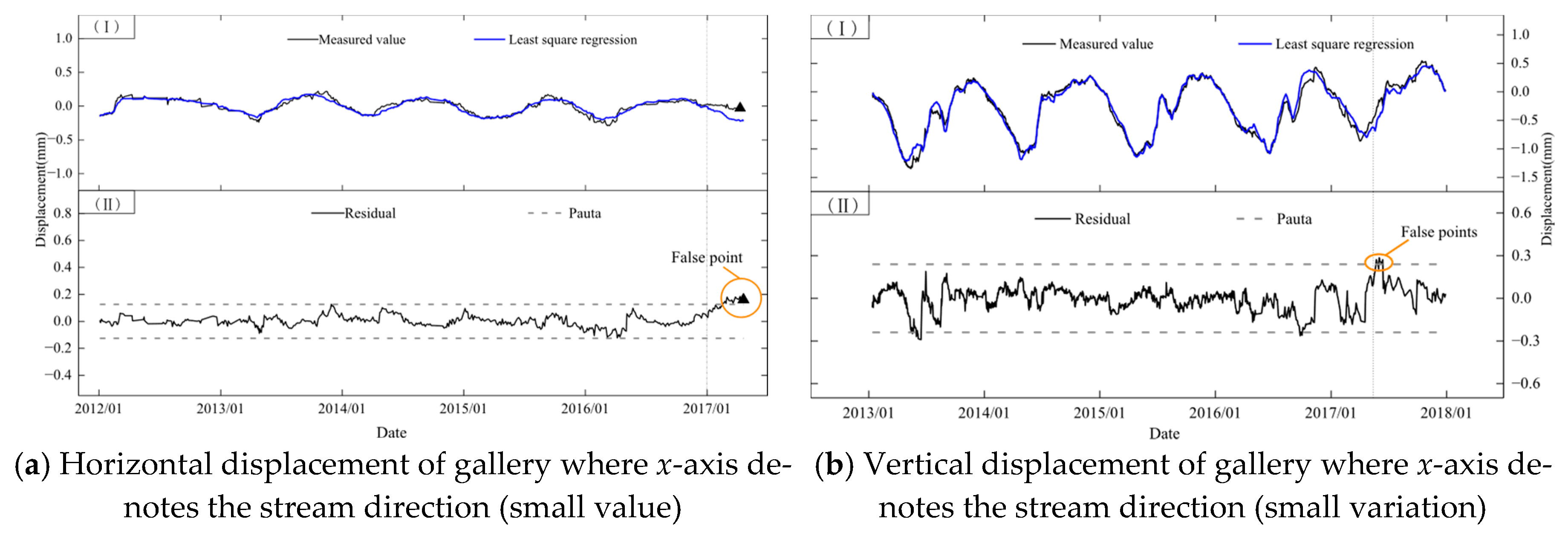
Due to the characteristics of response data, monitoring instrument modification, instrument range adjustment, etc., “small-value” observations are common in dam safety monitoring. The “small-value” observations usually have small monitoring values and small variations, such as observations of fractures and dislocations. This type of data sequence can be well fitted by a least squares regression. However, the magnitude of the estimation error is close to or even larger than the early warning threshold of the Pauta criterion. Therefore, the estimation error between the sample and the population cannot be ignored. The Pauta criterion does not take into account this estimation error, which would result in a small-value early warning threshold and cause misjudgments of normal values, as shown in Figure 5.

3. Improved Method of Early Warning Threshold Setting

Besides step-type and oscillatory-type anomalies, outliers are also common in dam safety monitoring data. The causes of outliers are complicated. Outliers cannot be eliminated directly; otherwise, it will have a negative effect on the engineering safety assessment. Since outliers are unavoidable in many cases, we propose an MZ criterion of early warning threshold setting for the identification of anomalies in dam safety monitoring data. The process of threshold setting comprises the following three main steps.

3.1. Establishing a Robust Regression Model of the Observations

The multivariate linear regression (MLR) model for anomaly identification of dam safety monitoring data can be expressed as [19]

$$Y=X\beta +\mu$$

(1)

where Y is the historical observation vector of $n\times 1$ and n is the sample size. X is the matrix of historical environmental variables with a dimension of $n\times k$, and k is the number of independent regression parameters in the model. $\beta$ is the k-dimensional unknown regression parameter vector, and $\mu$ is the random error term which is assumed to have an independent and identical distribution of $\mu ~N\left({\sigma }_{\mu }\right)$ [20].

The least squares method has been widely used to perform multivariate linear regression (MLR) and calculate the coefficient vector by minimizing the sum of the squares of the residuals. When there are many outliers in the observations, the regression line will be “pulled” by the outliers, resulting in low-accuracy results. The robust estimation can make full use of the valid information of the observations and avoid the influence of outliers as much as possible in order to obtain the best estimates. In this paper, the M-estimator, first introduced by Huber [21], is employed to solve the robust regression problem. Thus, the estimation of the coefficient vector of the M-estimator ${\widehat{\beta }}_{\mathrm{M}}$ can be expressed as

$${\widehat{\beta }}_M=arg\underset{\beta }{\min }\sum _{i=1}^n\rho \left({\displaystyle \frac{r_i}{s}}\right)$$

(2)

where $r_i$ is the residual for the i-th observation, defined as r_i = y_i − x_i^Tβ, and s is a scale estimate of the residuals. The weight function $\mathsf{\omega }\left(\mathrm{u}\right)$ is used to assign weights to each residual based on its magnitude.

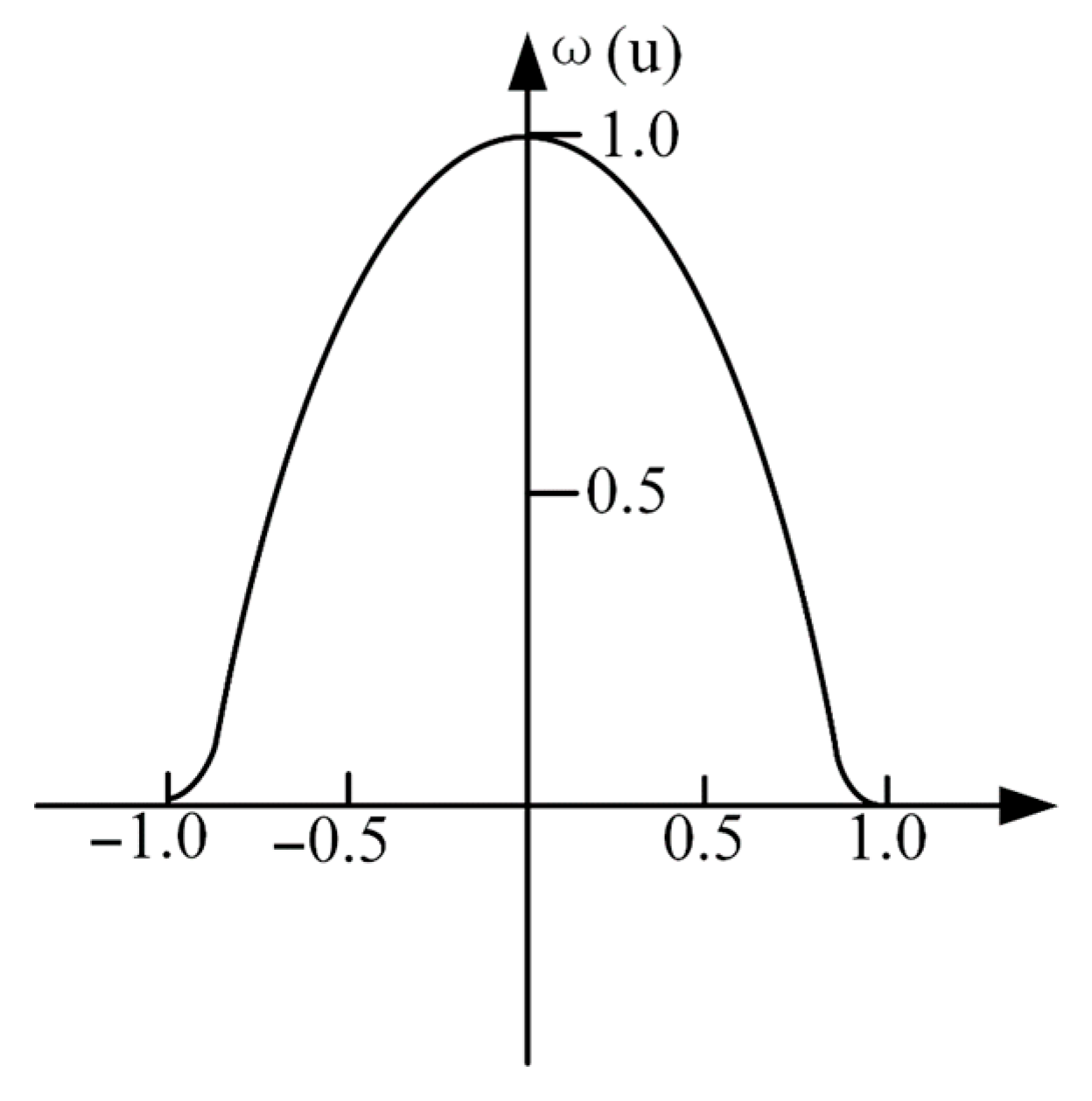
Different types of M-estimators have been proposed by Huber [22], Andrews and Hampel [23], Hampel [24] and Tukey [25]. The estimation of the Huber M-estimator is close to the sample average, but its robustness is inadequate. The derivative function of the objective function of the Hampel regression estimator is complicated and rarely applied in practical engineering. The Andrews estimator and the Tukey double-weight estimator divide the measurement interval into an elimination area and a useful area and are widely used in various fields. The Tukey M-estimator was selected in this paper because of its wider derivative function of the objective function and strong resistance. The objective function and weight function of the Tukey M-estimator are shown in Figure 6 and Figure 7, respectively. The objective function of the Tukey biweight estimator is denoted as ρ(u). Among various types of M-estimators, the Tukey biweight estimator stands out due to its strong resistance and smooth objective function. Its objective function ρ(u) and weight function $\mathsf{\omega }\left(\mathrm{u}\right)$ are defined as follows:

$$\mathsf{\rho }\left(\mathrm{u}\right)=\left\{\begin{array}{cc}{\mathrm{c}}^2\left(1-{\left(1-{\left({\displaystyle \frac{\mathrm{u}}{\mathrm{c}}}\right)}^2\right)}^3\right)& if\left|\mathrm{u}\right|\le c\hfill \\ {\mathrm{c}}^2\hfill & \hfill if\left|\mathrm{u}\right|>c\end{array}\right.$$

(3)

$$\mathsf{\omega }\left(\mathrm{u}\right)=\left\{\begin{array}{cc}{(1-{({\displaystyle \frac{\mathrm{u}}{\mathrm{c}}})}^2)}^2& \hfill if\left|\mathrm{u}\right|\le c\hfill \\ 0\hfill & \hfill if⌈\mathrm{u}⌉>c\end{array}\right.$$

(4)

where $\mathrm{c}$ is a tuning constant that determines the robustness and efficiency of the estimator. The choice of $\mathrm{c}$ is crucial as it balances the trade-off between robustness and efficiency. Typically, $\mathrm{c}$ is set to 4.685 to achieve 95% efficiency for the normal distribution. The tuning constant c is set to 4.685, a standard value in robust estimation that ensures efficiency for normal distributions while providing robust outlier resistance.

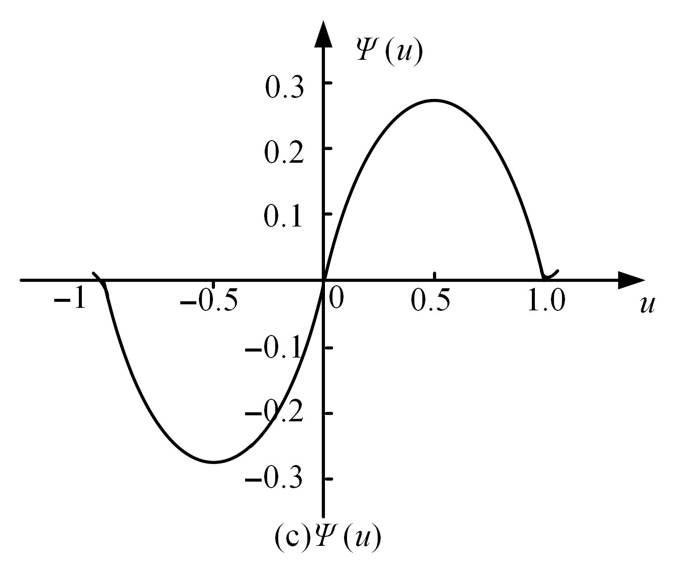
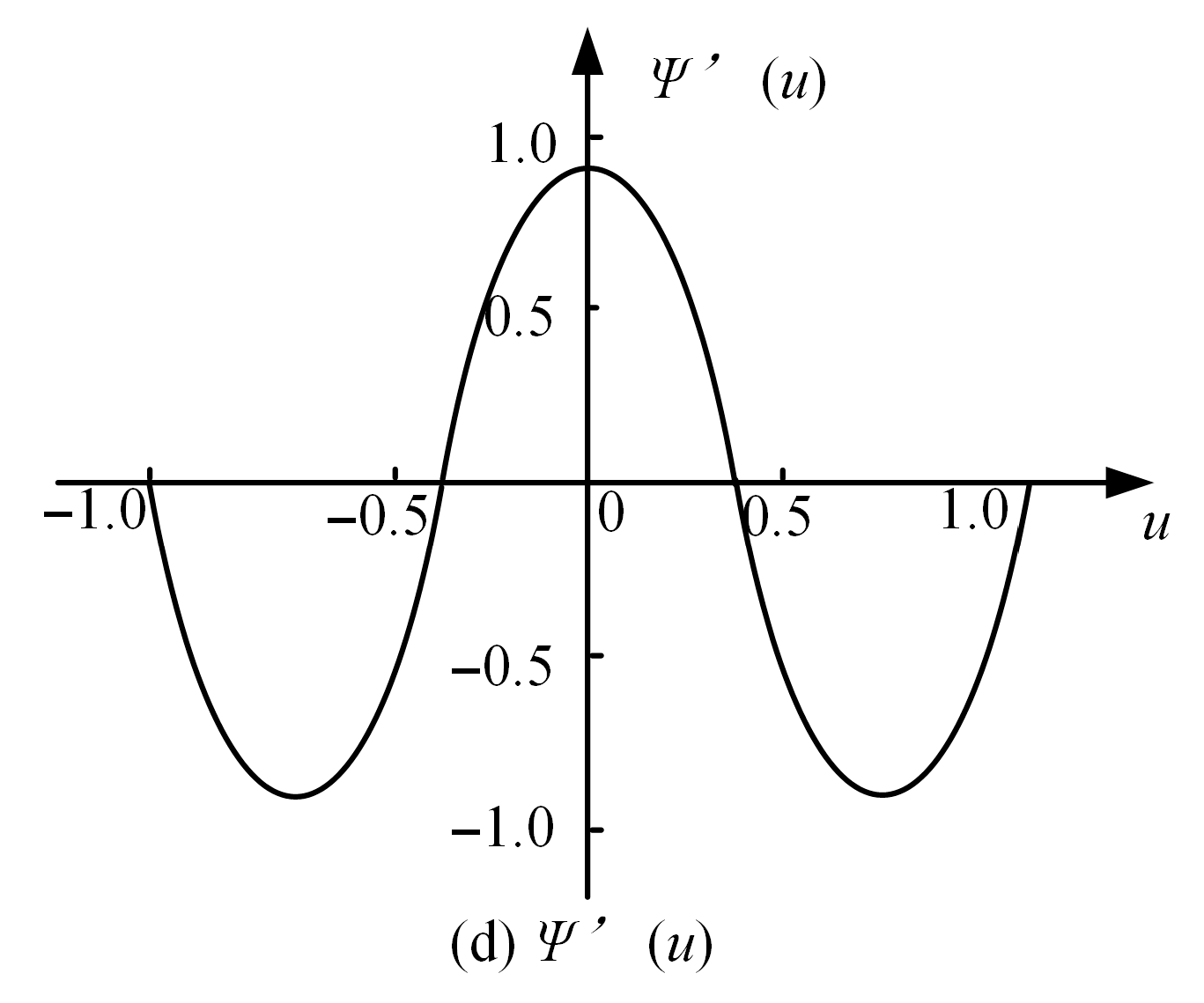
To further understand the properties of the Tukey biweight estimator, we introduce the first and second derivatives of the objective function, $\Psi \left(\mathrm{u}\right)$ and ${\Psi }^{\prime }\left(\mathrm{u}\right)$, which play important roles in the estimation process and provide insights into the behavior of the estimator. Figure 8 and Figure 9 illustrate the graphical representations of $\Psi \left(\mathrm{u}\right)$ and ${\Psi }^{\prime }\left(\mathrm{u}\right)$, respectively.

It can be seen that different weights are given according to the distance between the measured value and the center of the sequence. The closer the distance is, the higher the weight given, and vice versa. The outliers only take very small weights, which can reduce the negative impact of outliers on statistical estimation and improve stability and resistance.

3.2. Calculating the Scale Estimator Based on the Location M-Estimator

The scale estimator S_T is a weighted estimator of the off-center trend of data. It gives different weights to data points according to their distance from the center in order to resist outliers. The general form of a scale estimator is expressed as

$$S_T={\displaystyle \frac{\left(cMAD\right)n^{\frac{1}{2}}{\left[\sum _{i=1}^n{\psi }^2\left(u_i\right)\right]}^{\frac{1}{2}}}{\left|\sum _{i=1}^n{\psi }^{\prime }\left(u_i\right)\right|}}$$

(5)

where $u_i={\displaystyle \frac{x_i-T_n}{cMAD}}$ is a standardized variable that ensures the location and the scale equivariance; $\psi (•)$ is the derivative function of the objective function; ${\psi }^{\prime }\left(•\right)$ is the derivation of $\psi (•)$; n is the sample size; x_i is the data sequence; c is the tuning constant coefficient; MAD is the median of the distance from each observation to their median, i.e., $MAD={median}_i\left\{\left|x_i-M\right|\right\}$, and M is the median of data sequence x_i; $T_n$ is the location M-estimator, which can be expressed as

$$T_n={\displaystyle \frac{\sum _{i=1}^n{x}_i\omega \left(\frac{x_i-T_n}{c{S}_n}\right)}{\sum _{i=1}^n\omega \left(\frac{x_i-T_n}{c{S}_n}\right)}}$$

(6)

where $\omega (•)$ is the weight function and $S_n$ is the auxiliary scale estimation with the median absolute deviation MAD.

3.3. Calculating the Confidence Interval Radius Based on the Robust Regression Model

The confidence interval of the predicted values is the central interval that contains sample estimates with a certain probability level (confidence level). It shows the probability that the measured value will fall around the predicted value. The confidence interval radius D based on the robust regression can be written as

$$D=t_{\alpha /2}{S}_T\sqrt{\left[1+\left({\omega }_0{X}_0\right){\left(X^{\prime }WX\right)}^{-1}{X}^{\prime }X{\left(X^{\prime }WX\right)}^{-1}{\left({\omega }_0{X}_0\right)}^{\prime }\right]}$$

(7)

where $t_{\alpha /2}$ is the probability quantile of the t-distribution at a certain confidence level of $1-\alpha$ and the online anomaly recognition threshold is set based on the Pauta criterion with a confidence of 99.7% in the prediction. W is the equivalent weight matrix, and the Huber weight function is used in this paper. $X_0$ is a matrix of real-time environmental variables, and ${\omega }_0$ is the real-time weight which can be calculated by

$${\omega }_0=\left\{\begin{array}{cc}{\left(1-u_0^2\right)}^2& , \left|u_0\right|\le 1\\ \hfill 0\hfill & , \left|u_0\right|>1\end{array}\right.,u_0={\displaystyle \frac{0.6745e_0}{median\left\{\left|Y_i-X_i{\widehat{\beta }}_{M,}\right| i=\mathrm{1,2},\dots ,n\right\}}}$$

(8)

where $e_0$ is the real-time prediction error of the model.

3.4. Establishing the Anomaly Early Warning Threshold

The anomaly early warning threshold is set as

$$-3S_T<Y_0-{\widehat{Y}}_0<3S_T+D$$

(9)

where $Y_0$ is the observations and ${\widehat{Y}}_0$ is the predicted values.

A measured value that satisfies Equation (7) is a normal value. Otherwise, it is an abnormal value.

The update mechanism of the weight matrix W in the confidence interval radius D calculation formula (Equation (5)) is as follows:

1. Initialization: W is initialized as an identity matrix W₀ = I before processing monitoring data.

2. Anomaly Proportion Calculation: For each new data batch, compute the outlier proportion p using the current MZ criterion threshold.

3. Weight Adjustment: Update W via the following formula:

$$W_{t+1}\left(i,j\right)=\left(1-p\right)\times W_t\left(i,j\right)+p\times \delta \left(i,j\right)$$

(10)

where δ (i, j) is the Kronecker delta (1 if i = j, 0 otherwise). These down-weight entries correspond to outlier indices.

4. Dynamic Iteration: For subsequent batches, repeat the process, with p dynamically updated based on real-time anomaly detection results.

4. Sensitivity Analysis

The accuracy and reliability of the MZ criterion depend on the stability of the robust regression model and the M-estimator. Thus, we focus on analyzing the effect of the proportion of outliers on the robust regression model and the M-estimator in this section.

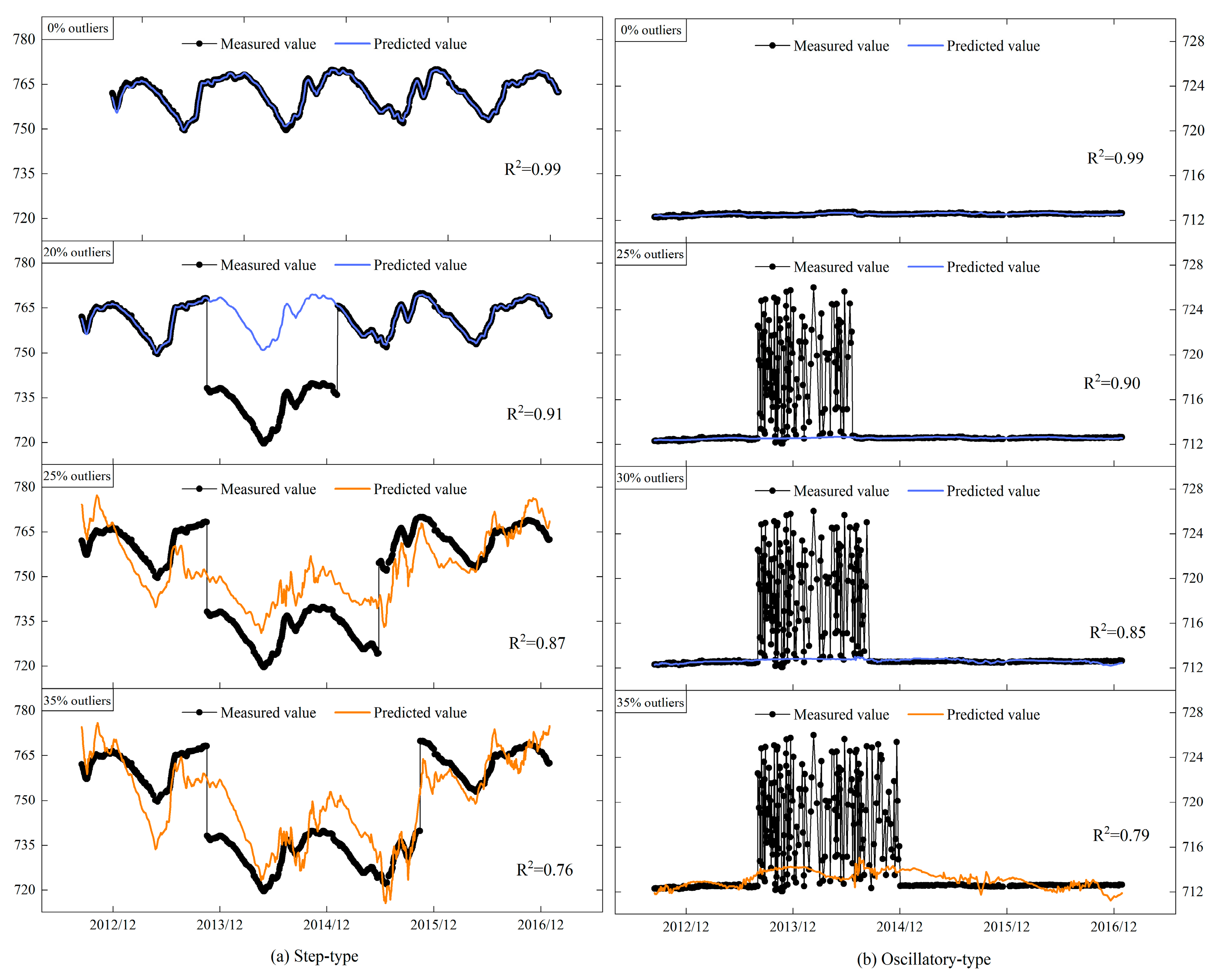
To further investigate the sensitivity of the robust regression model and the M estimator to outliers, we took two sets of observations for analysis; one was periodic, while the other was relatively stable. Outliers were added to make the proportion of outliers be 5%, 10%, 15%, 20%, 25%, 30%, and 35%. The results are shown in Figure 10. 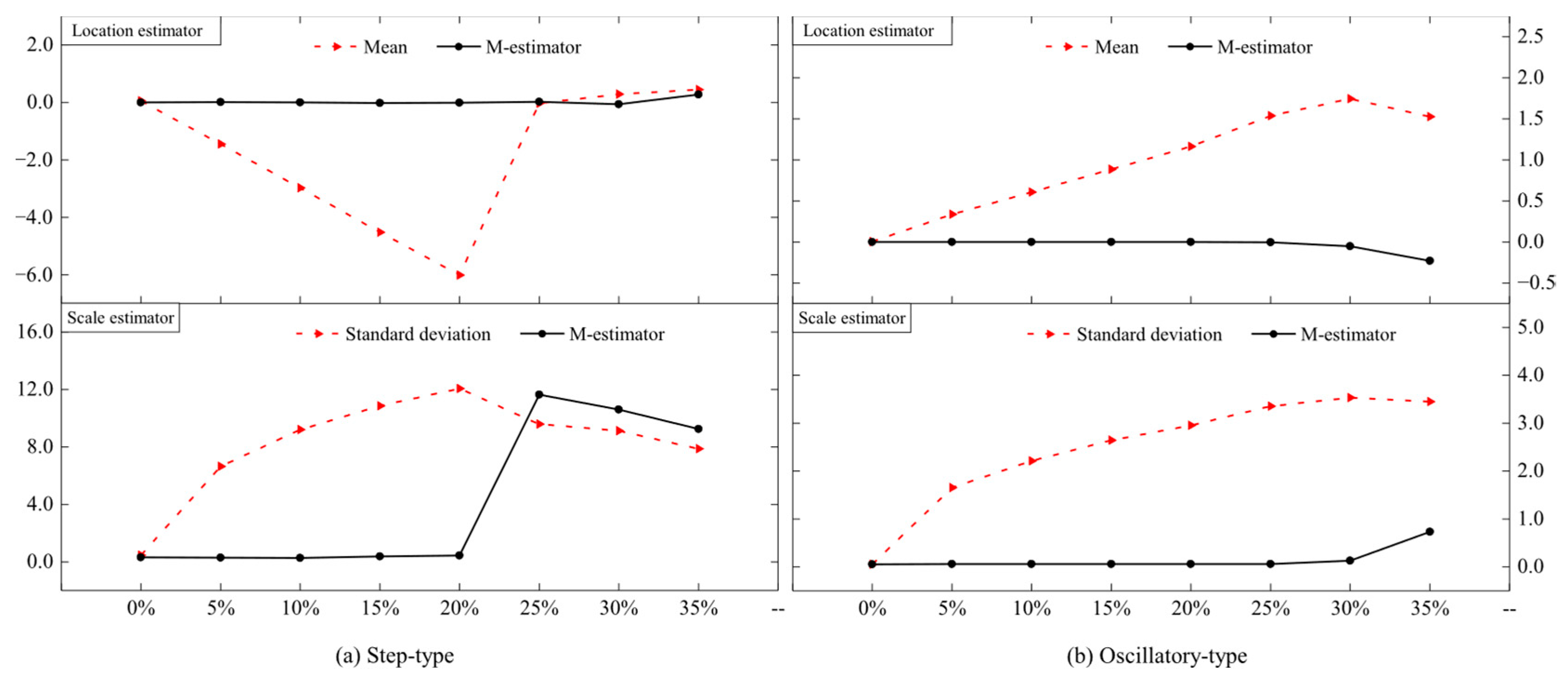Figure 10 includes R² values for curves, demonstrating that the MZ criterion maintains high goodness-of-fit (R² > 0.75) even in datasets with substantial outliers. The results show that the robust regression model can maintain good robustness when confronting step-type outliers up to 25% and oscillatory-type outliers up to 30%. This indicates that the model has a significant advantage in processing data sequences with substantial outliers. The stability and tolerance of the M-estimator are better than that of the least squares estimator under different proportions of outliers. If the data sequences do not contain outliers, the two estimators can obtain similar results. As the number of outliers increases, the mean and standard deviation of the least squares estimates deviate further from their true levels, while the M-estimator can tolerate the perturbation of about 20% of the outliers, as shown in Figure 11. In field applications, the outlier proportion can be monitored via moving window MAD calculations. When >20% of windows exhibit abnormal MAD values, data segmentation is recommended to maintain threshold accuracy.

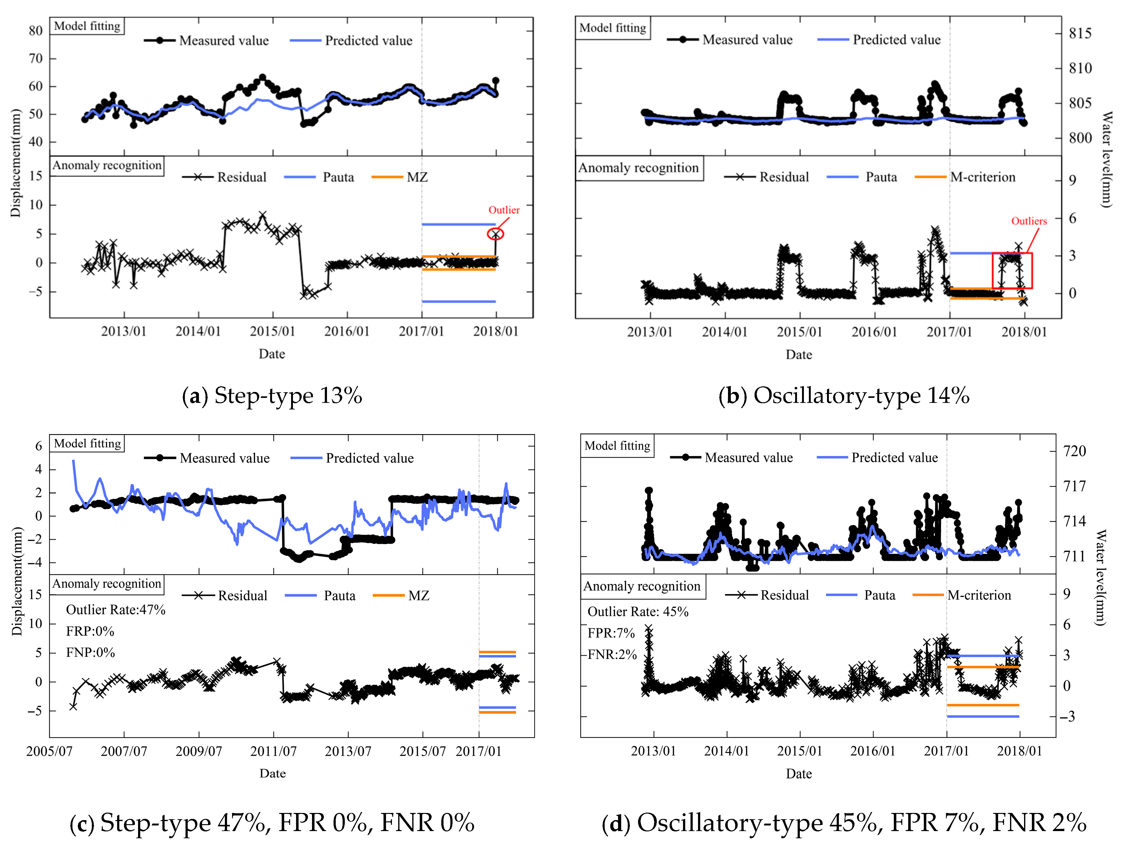
Based on the statistical analysis, the MZ criterion proposed in this paper can resist the influence of outliers within 20% and has good resistance and robustness, as shown in Figure 12a,b. Figure 12c,d display quantitative indicators, showing that the MZ criterion achieves 7% error rates even at 45% outliers, significantly outperforming traditional methods with >20% error rates. However, if the proportion of outliers is too large, both the robust estimation model and the MZ criterion will fail, as shown in Figure 12c,d. Then, we can divide sequences into segments and set the early warning threshold separately in order to improve the accuracy of the identification model. The flowchart for outlier identification is shown in Figure 13.

5. Application in Engineering

The XB Hydropower Station, located in the southwest of China, is a roller-compacted concrete arch dam primarily designed for power generation, with a maximum height of 141.5 m and an installed capacity of 240 MW. The crest elevation of the arch dam is 1409.50 m, with a maximum height of 141.50 m, a crest length of 434.46 m, a crest width of 8.00 m, and a thickness at the base ranging from 35 to 38 m. The location map is shown in Figure 14.

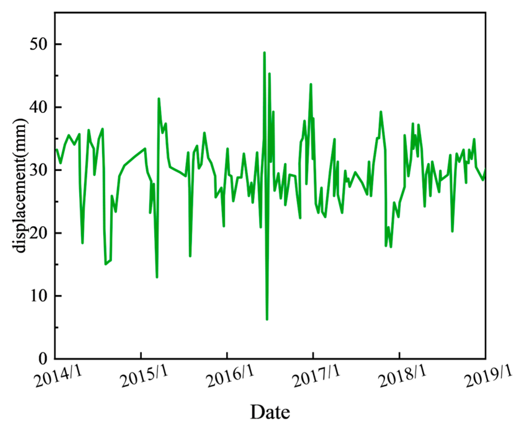
A large number of monitoring instruments have been installed in the dam body, dam foundation, downstream of the dam, and on both banks to monitor the safe operation of the dam. This study selects displacement and seepage monitoring data as the research objects to verify the effectiveness of the anomaly identification model based on the MZ criterion. The research data, as shown in Figure 5, covers the monitoring period from 2014 to 2018.

The MZ criterion, proposed in this study for setting early warning thresholds in anomaly identification, has been successfully implemented in the online safety monitoring systems of the XB Hydropower Station. Automatic monitoring has been implemented in these dams, and the data acquisition system has been equipped with functions of missing instrument identification and abnormal instrument discrimination, which can ensure the accuracy and reliability of the data acquired to a certain extent. To further validate the effectiveness of the MZ criterion proposed in this paper and its universality across different dam types, we additionally analyzed 94,241 safety monitoring records (2014–2018) from 259 observation points at GZ and TJZ Dams as an extended case study. We used two mathematical models to perform online anomaly identification; one was based on the Pauta criterion, and the other was based on the proposed MZ criterion. The results obtained from the two mathematical models were then compared with those from manual identification.

To prevent the trending changes in monitoring data from adversely affecting anomaly detection, the paper extracts the residual components of displacement at GZ and TJZ dams as the data basis for anomaly detection, with the extraction results shown in Figure 15 and Figure 16.

The residuals’ distribution indicates that the model can effectively capture the main trends and changes in the data. Using the MZ criterion for residual analysis enables more accurate anomaly detection, thus enhancing the accuracy and reliability of anomaly identification.

In the model, environmental variables such as water temperature and dam temperature field were considered for their correlation with monitoring data. Statistical tests showed that water temperature fluctuations caused 12–18% of displacement data variations, while non-uniform temperature fields induced anomalies in 8–15% of seepage pressure measurements. This quantitative assessment clarifies how environmental factors influence anomaly identification.

In previous research, the MZ criterion was confirmed to exhibit lower false positive and false negative rates compared to M-robust regression [18]. This characteristic is also demonstrated in its comparison with the Pauta criterion.

Table 1. Anomaly identification results of dam safety monitoring data in GZ and TJZ dam.

Anomaly Identification Model	Data Type	Mutations	Alarms	Misjudgments	Omissions	Misjudge and Omission Rate (%)
Anomaly identification model based on the Pauta criterion	Disp.	4	72	0	0	0
	Seepage	8	270	1316	6	2.48
Anomaly identification model based on the MZ criterion	Disp.	4	76	0	4	0.01
	Seepage	25	1495	94	9	0.19
Manual identification	Disp.	4	72	Total	Disp.	40,905
	Seepage	25	1580		Seepage	53,336

and

Table 2. Results of mutation identification in GZ and TJZ dam.

Dam	Observation Point	Number of Observations	Number of Anomalies Identified by the Pauta Criterion	Number of Anomalies Identified by the MZ Criterion	Number of Anomalies Identified Manually	Misjudgments	False and Missing Alarm Rate (%)
GZ	YY741	670	10	11	11	1	0.15
	YY813	670	21	46	46	25	3.73
	YY10101	671	28	87	87	59	8.79
TJZ	YY17-3	652	5	8	8	3	0.46
	LSY19	660	7	21	21	14	2.12
	LSY12	671	21	94	94	73	10.88

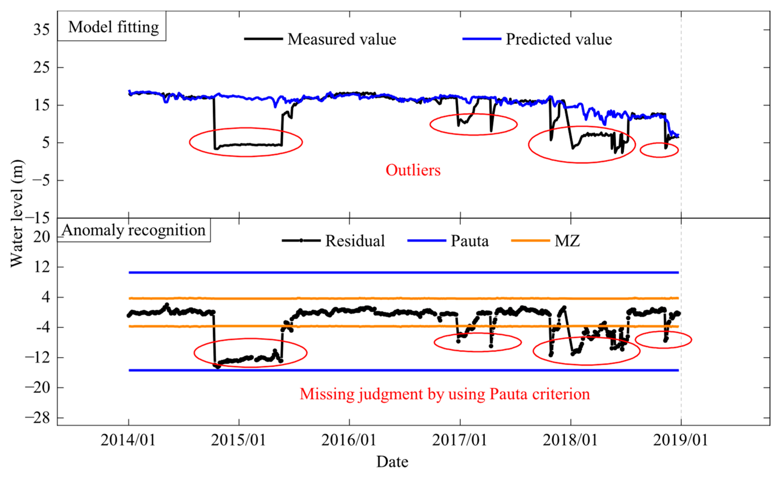
, respectively, show the anomaly identification results of the two mathematical models based on the Pauta criterion and the MZ criterion in the safety monitoring data of GZ and TJZ dam. It can be seen from Table 1 that the model based on the Pauta criterion caught 12 abnormal mutation points and missed 17 mutation points. About 342 anomalies were caught, 1316 anomalies were missed and 6 anomalies were misjudged. The overall misjudge-and-omission rate was up to 2.48%. Misjudgments and omissions mainly exist in seepage sequences that were usually step-type and oscillatory-type, as shown in Figure 17 and Figure 18. For single observation points, the false and missing alarm rate is as high as 10%, as shown in Table 2.

Therefore, for both observation point groups and single observation points, the identification method based on the MZ criterion can maintain a low false and missing alarm rate and a high recognition accuracy, especially for the step-type and oscillatory-type data sequences that often occur in dam safety monitoring data.

6. Conclusions

The study presents an innovative solution for anomaly warning thresholds in dam safety monitoring data, known as the MZ criterion. Conventional models grounded in the Pauta criterion often fall short when dealing with step-type, oscillatory-type and small-value data. Their effectiveness is hindered by heightened sensitivity to outliers and a rigid reliance on specific data distribution patterns. The MZ criterion, a hybrid model incorporating the scale estimator ST (based on the location M-estimator) and the confidence interval radius D from robust regression, has been developed to address these limitations.

Extensive testing has shown that the MZ criterion exhibits remarkable robustness against outliers, maintaining its efficacy as long as the proportion of outliers remains within 20%. Its particular strength lies in online anomaly identification within challenging data types, where it has proven to be especially reliable. When applied to the online safety monitoring system of dams in the Dadu River Basin, the MZ criterion demonstrated impressive performance. It consistently achieved low rates of misjudgment and omission while delivering high recognition accuracy across both grouped and individual measuring points. This makes it a highly effective tool for monitoring step-type and oscillatory-type data, which are commonly encountered in dam safety monitoring scenarios.

Although the method may face challenges and potentially fail when the proportion of outliers exceeds 20%, a practical solution is available. By segmenting data sequences and setting thresholds individually for each segment, the performance of the MZ criterion can be significantly enhanced. Overall, the MZ criterion represents a substantial advancement in the field of online dam safety monitoring. It provides a more reliable data support system, effectively reducing the rate of false and missed alarms for anomalies to within 2%. This makes it a valuable tool for enhancing the safety and reliability of dam operations.