Impact of Data Quality on CNN-Based Sewer Defect Detection

Abstract

Sewer pipelines are essential urban infrastructure that play a key role in sanitation and disaster prevention. Regular condition assessments are necessary to detect defects early and determine optimal maintenance timing. However, traditional visual inspection using closed-circuit television (CCTV) footage is time-consuming, labor-intensive, and dependent on subjective human judgment. To address these limitations, this study develops a convolutional neural network (CNN)-based sewer defect classification model and analyzes how data quality—such as mislabeled or redundant images—affects model accuracy. A large-scale public dataset of approximately 470,000 sewer images was used for training. The model was designed to classify non-defect and three major defect categories. Based on the ResNet50 architecture, the model incorporated dropout and L2 regularization to prevent overfitting. Experimental results showed the highest accuracy of 92.75% at a dropout rate of 0.2 and a regularization coefficient of 0.01. Further analysis revealed that mislabeled, redundant, or obscured images within the dataset negatively impacted model performance. Additional experiments quantified the impact of data quality on accuracy, emphasizing the importance of proper dataset curation. This study provides practical insights into optimizing data-driven approaches for automated sewer defect detection and high-performance model development.

1. Introduction

Sewers are essential urban infrastructure, playing a critical role in public sanitation and stormwater management. However, the deterioration of aged sewers has emerged as a significant concern in many countries [1]. The main causes of sewer deterioration include long-term degradation of material properties, poor construction, root intrusion, heavy traffic loads, structural deformation due to ground settlement, infiltration of groundwater, and crown corrosion from bio-chemical reaction [2,3,4]. These deteriorations can lead to defects such as cracks, fractures, and joint dislocations in sewer pipelines, which may ultimately cause severe issues such as reduced flow capacity, flooding, and sinkholes. Such problems can be prevented by determining the timing for sewer rehabilitation in advance through regular condition assessments. Sewer condition assessments are conducted using various evaluation protocols like the pipeline assessment certification program (PACP) developed by the National Association of Sewer Service Companies, commonly known as NASSCO [5,6]. After inspection, a condition grade is assigned to each sewer segment based on the protocol, which in turn determines the priority for rehabilitation. These condition assessment protocols generally consist of the following steps: collecting sewer information, identifying and assessing defect severity, and generating an evaluation report [1,7,8].

Sewer data collection methods can generally be classified into visual, laser profiling, and sonar techniques [9]. Among these, visual inspection using CCTV video recording is the most commonly used method due to its operational simplicity. The recorded images are analyzed by experts through visual observation to identify defects, and this method relies entirely on human interpretation. However, such human-dependent approaches are time-consuming and costly, and they suffer from reduced detection accuracy due to inspector fatigue. Furthermore, the results may vary depending on the inspector’s experience and subjective judgment [10]. To overcome these limitations, it is necessary to develop technologies that can automatically detect sewer defects, thereby reducing the need for human intervention and enabling more objective and quantitative assessments [7,11,12].

With recent advances in artificial intelligence (AI) technology, AI-based approaches have been actively studied in the field of image analysis. One area of research for automating the analysis of images is computer vision [13,14,15]. This technique enables the acquisition, processing, and analysis of images by AI. However, it is sensitive to lighting conditions, surface contamination, and the variability of defect types, which can lead to inconsistent detection accuracy and difficulty in effectively identifying complex defects [8,12,16].

Convolutional neural networks (CNNs), a subfield of deep learning (DL), have demonstrated excellent performance in image analysis and have been widely applied in fields such as autonomous driving and face recognition [17]. CNN-based automation research has also been conducted for sewer defect detection [8,12,18]. These studies have employed techniques such as dropout [12], data augmentation [8], and image preprocessing using polar coordinate transformation [18] to prevent model overfitting due to limited data. Many prior studies in sewer defect detection have relied on relatively small datasets or architectures that decouple feature extraction and classification stages. Such approaches inherently limit model adaptability to complex defect patterns and diverse real-world inspection conditions [19]. To address these limitations, recent efforts have increasingly focused on end-to-end deep learning frameworks that integrate the entire inference pipeline into a unified model [20].

End-to-end object detection models such as YOLOv3 and Faster R-CNN have demonstrated strong performance in real-time applications, achieving mean average precision (mAP) scores ranging from 76.2% to 85.7% [7,21,22]. Moreover, the incorporation of attention mechanisms, including lightweight modules such as the Channel-Spatial Attention Module (CBAM), has been shown to further improve detection performance in complex visual environments [23]. Enhanced architectures such as CSA-MaskC-RCNN [22] and compact neural networks [24] are also being actively explored to improve model generalizability and field applicability [25].

While acknowledging these advancements, the present study employs a conventional CNN-based image classification model rather than an end-to-end detection approach. This decision is primarily due to the characteristics of the dataset used in this study, which lacks spatial annotations such as bounding boxes required for object detection. Instead, the dataset provides only image-level defect labels, making classification-based architectures (e.g., ResNet, VGG) more appropriate for the problem setting.

To this end, we utilized a large-scale sewer inspection image dataset provided by AI-Hub [26], a national open-data platform operated by the National Information Society Agency (NIA) of Korea. AI-Hub offers diverse, high-quality datasets for artificial intelligence training across multiple industries. Previous studies using AI-Hub datasets have reported high classification accuracy in domains such as vehicle identification [27] and fruit quality grading [28], achieving over 98% accuracy with more than 60,000 images. Building on these precedents, our study adopts a substantially larger dataset of approximately 470,000 images to enhance model robustness under operational conditions.

This study offers the following contributions:

• Development of a large-scale, image-based sewer defect classification model that outperforms conventional manual inspection methods in terms of accuracy and scalability.
• Demonstration of model optimization through hyperparameter tuning, including dropout rate and L2 regularization, resulting in statistically significant performance improvements.
• Identification of data quality issues—such as mislabeled and duplicated defect images—as critical factors affecting model performance, supported by a systematic misclassification analysis.
• Quantitative evaluation showing that a higher proportion of low-quality images within a dataset negatively impacts model accuracy, thereby providing empirical evidence of the relationship between data quality and model performance.
• Proposal of a data curation strategy that involves early-stage filtering of ambiguous or noisy images and expert validation, contributing to the construction of a more reliable and domain-consistent dataset for sewer infrastructure assessment.

These contributions are expected to serve as a foundation for advancing automated, data-driven sewer condition monitoring systems and overcoming limitations associated with labor-intensive visual inspection practices.

In this study, a CNN model was trained using the large-scale sewer pipeline image dataset provided by AI-Hub, resulting in the development of a high-accuracy defect detection model for sewer pipelines. Additionally, the quality of the training data was evaluated based on factors such as mislabeling, duplicate defect images, and image censorship. The impact of data quality on detection performance was analyzed accordingly. Finally, through additional experiments involving varying proportions of low-quality data, the effect of data quality on model performance was quantitatively assessed, leading to the proposal of an effective data construction strategy.

2. Materials and Methods

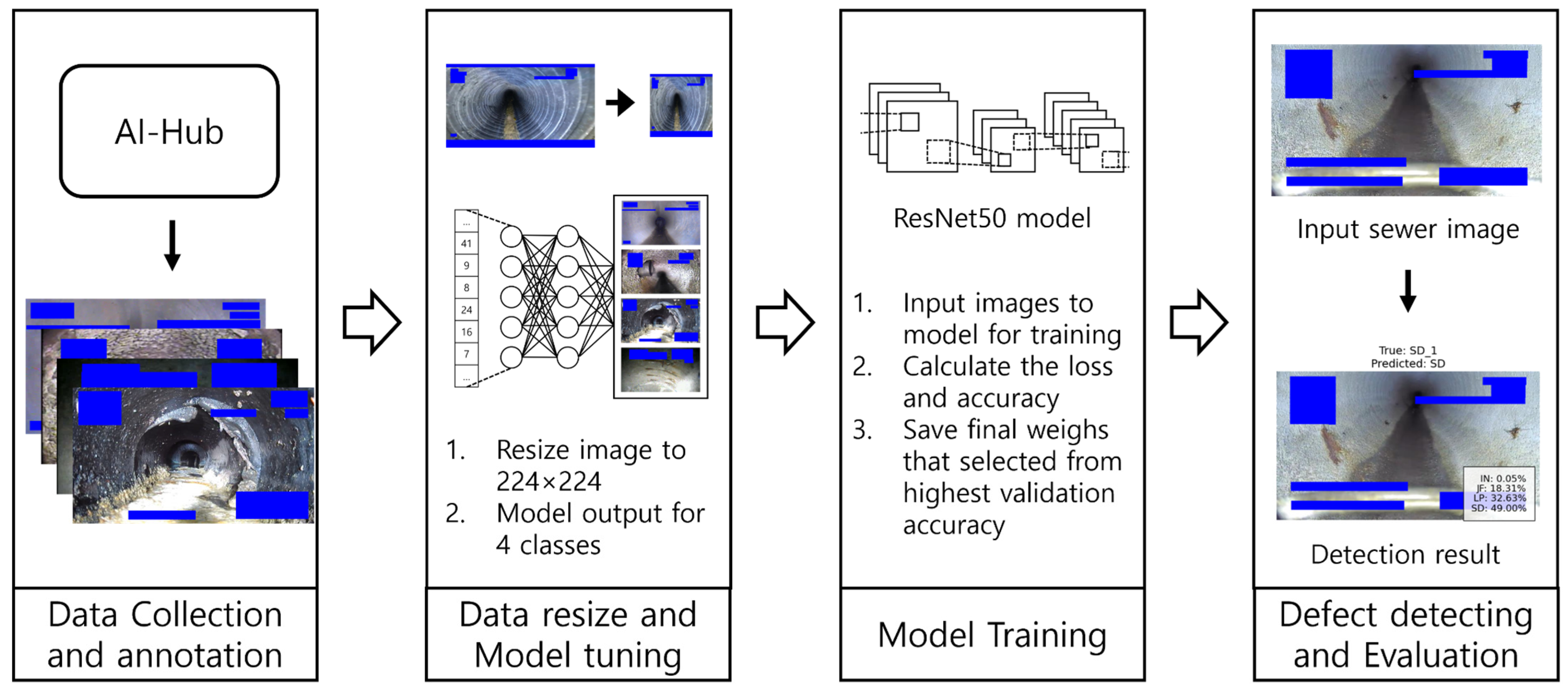
Figure 1 provides an overview of the proposed sewer pipeline defect detection model developed in this study. A defect detection for sewer pipelines was developed using a CNN-based ResNet50 architecture. ResNet50 is a deep neural network composed of 50 layers, incorporating the concept of residual learning to mitigate the vanishing gradient problem and enhance training performance. ResNet50 has demonstrated superior performance compared to conventional architectures such as AlexNet, ResNet-18, and ResNet-34 in prior studies addressing single-image-based sewer water level estimation tasks [29]. This result highlights the robustness of deeper convolutional neural networks in handling complex and noise-prone sewer CCTV imagery. Based on this evidence, ResNet50 was adopted in the present study as a suitable architecture for image classification under varying quality conditions.

Based on sewer pipeline image data collected from AI-Hub, the images were preprocessed to a resolution of 224 × 224 pixels and used to train a CNN model for classification into four defect categories. The model architecture was built upon ResNet50, and it was designed to output classification results for each category upon receiving test image inputs. The entire process is described in detail in the following subsections.

2.1. Dataset

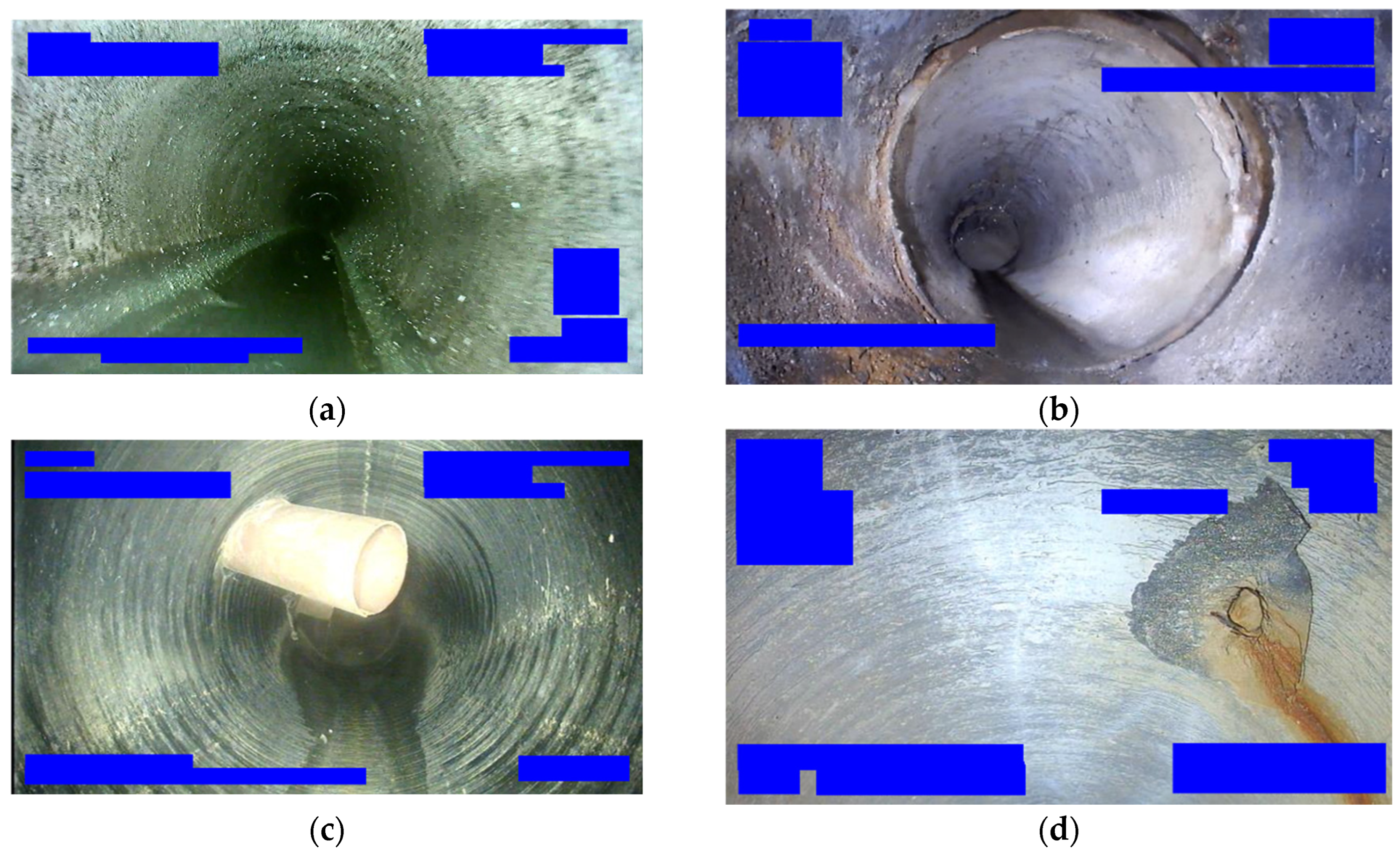
In this study, internal sewer pipe images from AI-Hub were utilized [26]. The platform provides a vast array of image data applicable to various industrial sectors such as autonomous driving, healthcare, manufacturing, environment, and construction. The dataset consists of approximately 470,000 images, categorized into eight defect types and three non-defect types. For this study, the selected classes for model classification include Normal-In (IN), Joint-Fault (JF), Lateral-Protruding (LP), and Surface Damage (SD), which are among the most frequently occurring defects [30]. These selected categories are illustrated in Figure 2.

High-resolution image data used in CNN training generally provide more detailed information, which can enhance model performance. However, training with high-resolution images also increases computational complexity and leads to longer training times. Typically, CNN models are trained using images ranging in size from 128 × 128 to 256 × 256 pixels [12]. In this study, the images were resized into a square format to match the model’s input requirements, and the resolution was set to 224 × 224 pixels. 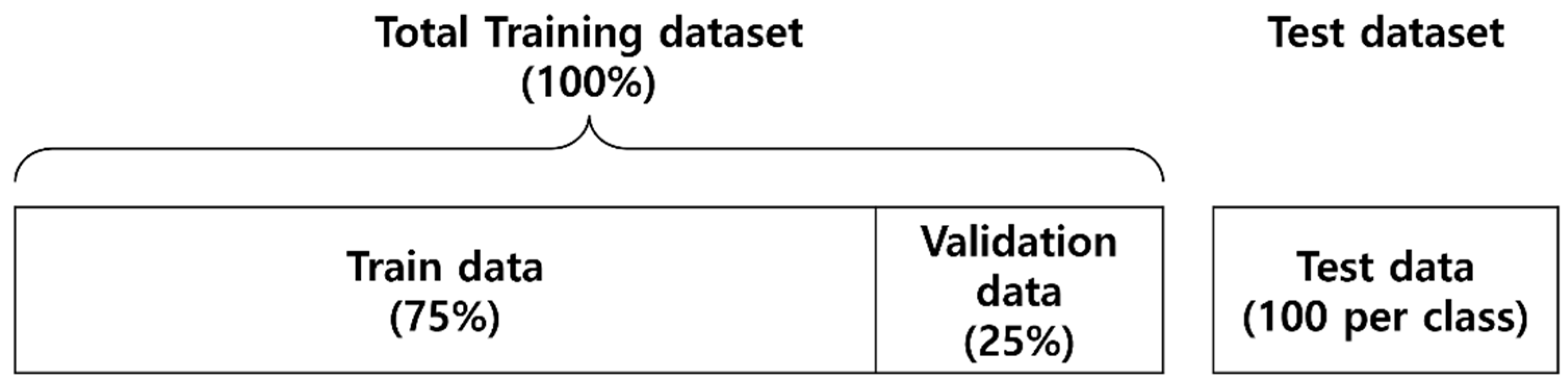As shown in Figure 3, 75% of the dataset was used as training data and 25% as validation data. The training dataset consisted of 10,000 images per class, totaling 40,000 images. For model evaluation, a separate test dataset was prepared with 100 images per class, totaling 400 images.

2.2. Computer System

Typically, deep learning models require large datasets for effective training. However, in specialized domains such as sewer pipeline defect detection, obtaining large-scale datasets can be challenging. Utilizing a pretrained model helps address data scarcity, facilitates faster convergence during training, and improves the model’s generalization capability [31]. The model weights were initialized using pretrained weights from the ImageNet dataset [32]. The model was implemented using Python 3.0 and the PyTorch (2.4.1) library. Training was conducted in a computing environment consisting of an Intel(R) Core(TM) i5-13400F CPU, NVIDIA GeForce RTX 4060 GPU, 16 GB RAM, Windows 10, and CUDA 12.6. The original fully connected layer of ResNet50, designed for 1000-class classification, was modified to output predictions for the four selected sewer defect categories in this study.

2.3. Model Evaluation

Model testing was conducted using a pre-prepared set of 400 test images. Each experiment was evaluated primarily based on the model’s accuracy. Accuracy refers to the proportion of correct predictions out of all predictions made and serves as a fundamental metric for assessing the overall performance of the model. Accuracy is calculated using the following formula:

$$Accuracy={\displaystyle \frac{TN+TP}{TN+TP+FN+FP}}$$

(1)

In the above equation, the terms are defined as follows:

TP (True Positive): The number of defect images correctly classified as defects.

TN (True Negative): The number of normal (non-defect) images correctly classified as normal.

FP (False Positive): The number of normal images incorrectly classified as defects.

FN (False Negative): The number of defect images incorrectly classified as normal.

The classification performance of the final trained model was evaluated using a confusion matrix, which provided detailed insights into class-wise prediction accuracy. To precisely analyze the model’s sensitivity to threshold variations, both the Receiver Operating Characteristic (ROC) curve and the Precision-Recall (PR) curve were examined. The ROC curve is a useful tool for assessing the model’s classification capability, with the Area Under the Curve (AUC) value approaching 1 indicating superior performance. The PR curve visualizes the relationship between precision and recall for different threshold settings, particularly for imbalanced datasets. The average precision (AP), defined as the area under the PR curve, also serves as a key indicator of model effectiveness, where higher values imply better performance. These evaluation metrics were comprehensively employed to assess not only the overall performance of the model but also its threshold-dependent behavior and prediction characteristics [33]. Finally, the misclassified images from the final model were analyzed, and the model’s performance was compared in relation to the quality of the training data.

3. Results and Discussion

3.1. Model Training

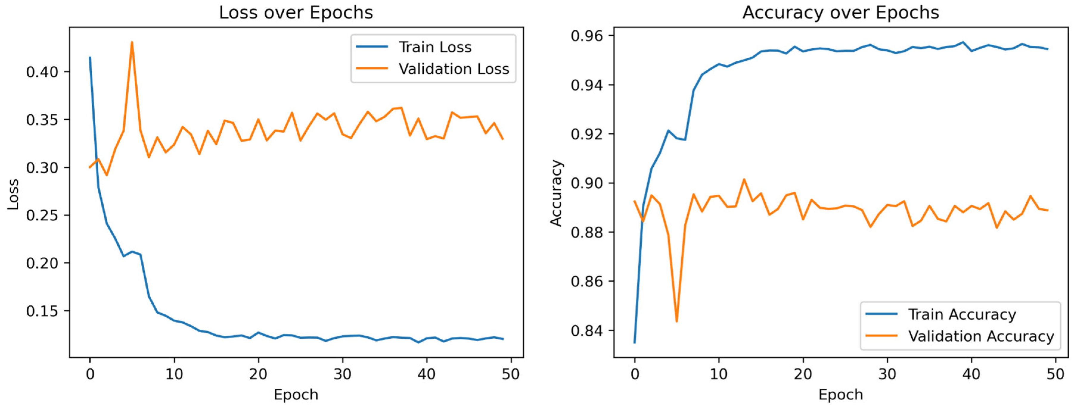
During model training, CrossEntropyLoss was employed as the loss function and Softmax as the activation function, both of which are well-suited for multi-class classification tasks. These functions enable optimal predictions by considering the probability distribution across multiple classes [34]. For optimization, Stochastic Gradient Descent (SGD) was utilized with a momentum of 0.9 to accelerate convergence [35]. To adjust the learning rate dynamically, a StepLR scheduler was applied, reducing the learning rate by a factor of 10 every seven epochs. This strategy maintained a rapid learning pace in the early stages while ensuring stable optimization in later phases [36]. Figure 4 visualizes the training process of the model. Training and validation steps were alternated in each epoch, and both loss and accuracy were recorded at every epoch. The final model weights were selected based on the epoch that yielded the highest accuracy on the validation dataset.

3.2. Hyperparameter Tuning

To optimize the performance of the sewer pipeline defect detection model, dropout and L2 regularization were selected as key hyperparameters and experimentally evaluated. These two techniques are well-known regularization methods that improve the generalization performance of neural network models.

Dropout is a regularization technique that probabilistically deactivates a portion of neurons in the network during training, preventing over-reliance on specific neurons and encouraging the learning of diverse features. While a low dropout rate may lead to overfitting, an excessively high rate can hinder the model’s learning capacity [37]. According to [37], dropout rates between 0.2 and 0.5 tend to yield optimal performance. In this study, dropout rates were adjusted within the 0.2 to 0.5 range to identify the optimal value. Additionally, a higher dropout rate of 0.8 was tested for comparative analysis.

L2 regularization is a technique that enhances model generalization by adding a penalty term to the loss function, which constrains the magnitude of the model’s weights and reduces unnecessary complexity [38]. It is typically implemented by including a regularization term in the loss function, as shown below.

$$L_{total}=L_{original}+\lambda \sum {\omega }^2$$

(2)

Here, λ is the regularization coefficient, a hyperparameter that determines the extent to which the model’s weights are constrained. By appropriately tuning this coefficient, overfitting can be mitigated, thereby improving model performance [38]. When applying L2 regularization to CNN models, λ values in the range of 0.0001 to 0.01 are generally considered appropriate [39]. In this study, the L2 regularization coefficient was adjusted within the range of 0.0001 to 0.1 to identify the optimal value.

Hyperparameters were tuned to optimize the performance of a CNN model for interpreting internal CCTV footage of sewer pipelines. The dropout rate and L2 regularization coefficient were adjusted to analyze their individual and combined effects on model performance. Experiments with varying dropout rates revealed that a rate of 0.2 yielded the highest accuracy at 90.25%. Dropout rates of 0.25, 0.35, and 0.8 maintained a similar level of performance; however, at other rates, the accuracy either showed negligible improvement or declined. This indicates that an optimal dropout rate exists depending on the structure of the CNN model and the size of the dataset.

Given the depth and complexity of the CNN architecture used, an appropriately configured dropout rate can help the model filter out irrelevant noise while effectively learning key features. In general, dropout tends to induce overfitting when too few neurons are involved in training, and underfitting when too many are dropped. Thus, the optimal dropout rate is influenced by the dataset size and the model architecture [37].

Applying dropout to datasets with fewer than 1000 images often led to decreased model performance, whereas datasets with more than 1000 images showed improved results with dropout [37]. However, for datasets exceeding 10,000 images, the effectiveness of dropout tended to diminish as the dataset size increased. The dataset used in this study consisted of 40,000 images, demonstrating a trend consistent with the findings of the previous study. The accuracy achieved for each dropout rate is presented in

Table 1. Effect of dropout rate on classification accuracy.

Dropout Rate	none	0.2	0.25	0.3	0.35	0.4	0.45	0.5	0.8
Accuracy (%)	88.25	90.25	88.75	88.00	89.50	88.00	88.50	87.50	89.75

.

The experimental results for different L2 regularization coefficients showed that the highest accuracy, 92.75%, was achieved when λ = 0.01. As the λ value increased, model performance gradually declined. Notably, when λ = 0.1, the accuracy dropped significantly to 78.00%. This decline is attributed to excessive regularization, which overly constrained the model’s weights and hindered effective learning.

Table 2. Impact of L2 regularization parameter (λ) on model performance.

L2 Ratio (λ)	none	0.0001	0.0005	0.001	0.005	0.01	0.05	0.1
Accuracy (%)	90.25	89.25	90.00	89.00	89.50	92.75	84.25	78.00

presents the visual trends and quantitative results of these experiments.

Ref. [39] found that the optimal L2 regularization coefficient was 0.00037. That study used relatively low-resolution datasets such as CIFAR-10 (32 × 32) and MNIST (32 × 32). In contrast, the dataset used in the present study consisted of high-resolution images (224 × 224), which may have necessitated a higher λ value. Furthermore, the LeNet-5 model used in [39] has approximately 60,000 parameters, while the ResNet50 model employed in this study has around 25.6 million parameters. This substantial difference in model complexity likely contributed to the differing optimal regularization values.

Given that ResNet50 is much deeper and more complex than LeNet-5, an appropriate level of L2 regularization is necessary to improve generalization. However, excessive regularization can limit the model’s representational capacity and ultimately degrade performance. Experiments were conducted by varying the dropout rate while fixing the L2 regularization coefficient at 0.01. The results showed that the highest accuracy (92.75%) was achieved when the dropout rate was set to 0.2. Although increased accuracy was also observed for other dropout rates such as 0.3, 0.35, 0.4, 0.5, and 0.8 after applying L2 regularization, the performance unexpectedly decreased when the dropout rate was set to 0.25 or 0.45.

These findings suggest that while dropout and L2 regularization play complementary roles, certain combinations can negatively impact model performance. L2 regularization constrains the magnitude of the weights, preventing the model from becoming overly complex, whereas dropout randomly disables certain neurons during training to reduce reliance on specific weights. Ref. [39] also reported that the combined application of dropout and L2 regularization is more effective in reducing overfitting compared to applying either technique alone.

The results of this study indicated that the combination of a dropout rate of 0.2 and an L2 regularization coefficient of λ = 0.01 yielded the highest performance. While this outcome is generally consistent with findings from previous studies, it was also observed that certain configurations—specifically, dropout rates of 0.25 and 0.45—led to a decrease in performance when both dropout and L2 regularization were applied simultaneously.

Table 3. Effect of dropout rate on classification accuracy with L2 regularization (λ = 0.01).

Dropout Ratio	L2 Regularization Ratio	Accuracy (%)
0.20	-	90.25
	0.01	92.75
0.25	-	88.75
	0.01	87.75
0.30	-	88.00
	0.01	89.50
0.35	-	89.50
	0.01	91.25
0.4	-	88.00
	0.01	89.50
0.45	-	88.50
	0.01	88.25
0.5	-	87.50
	0.01	89.25
0.8	-	89.75
	0.01	91.75

presents the visual patterns and quantitative results of these experiments.

3.3. Impact of Dataset Quality on Model Performance

The quality of the training dataset plays a critical role in the generalization performance of CNN-based sewer defect detection models. In this section, misclassified images were analyzed based on the final model, which achieved an accuracy of 92.75%, and it was confirmed that low-quality data were included in the training dataset. Additional experiments were conducted by varying the proportion of low-quality data within the training set to evaluate the impact of dataset quality on model performance.

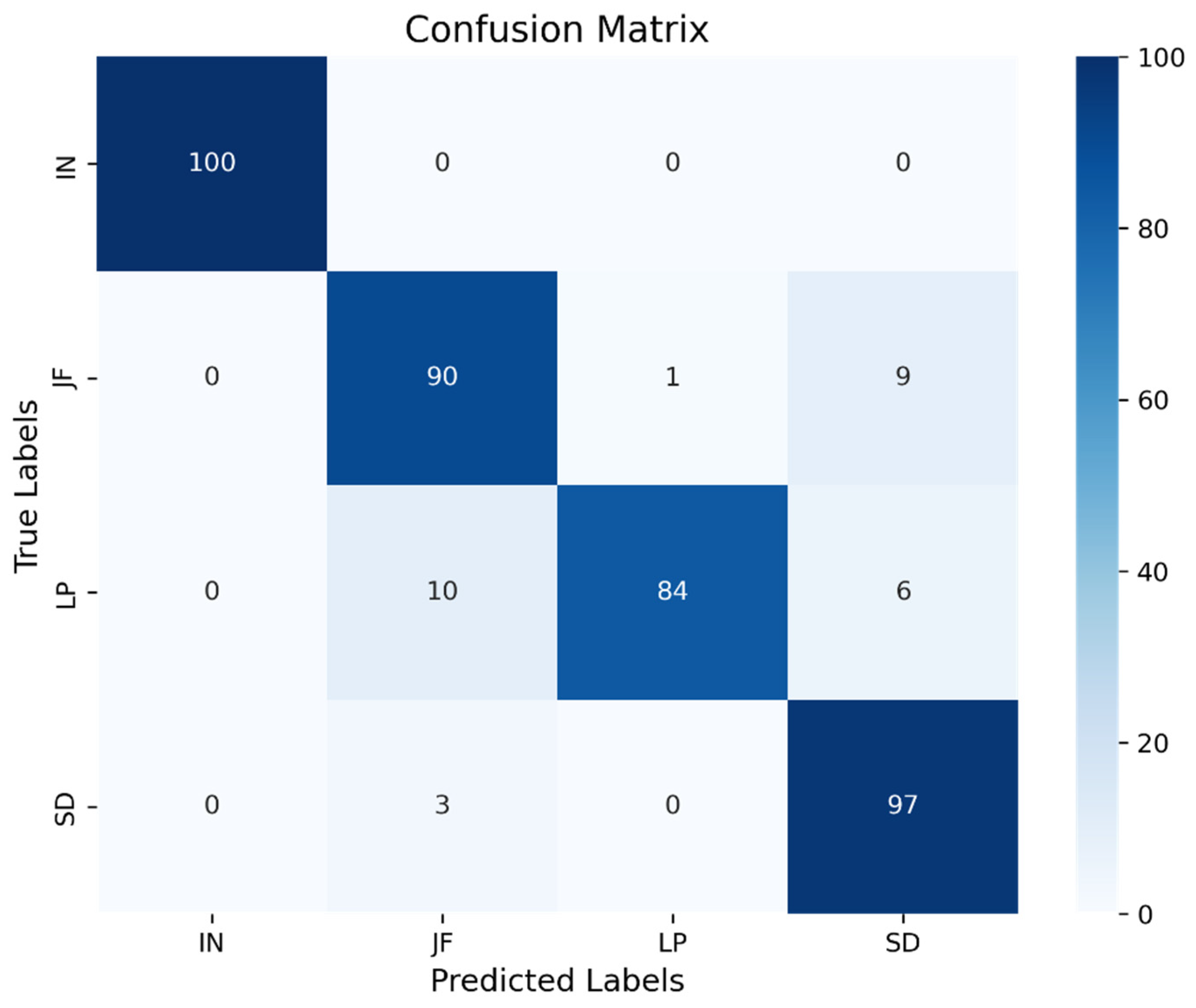
As shown in Figure 5, analysis of the model’s confusion matrix revealed variations in classification accuracy across different classes. The normal (IN) class achieved 100% accuracy, while the surface damage (SD) class showed a high accuracy of 97%. In contrast, the joint failure (JF) and lateral protrusion (LP) classes demonstrated comparatively lower accuracies of 90% and 84%, respectively. Although the model exhibited strong overall performance, these results highlight performance discrepancies across different classes. To quantitatively support these findings, additional analyses were conducted using the ROC and PR curves.

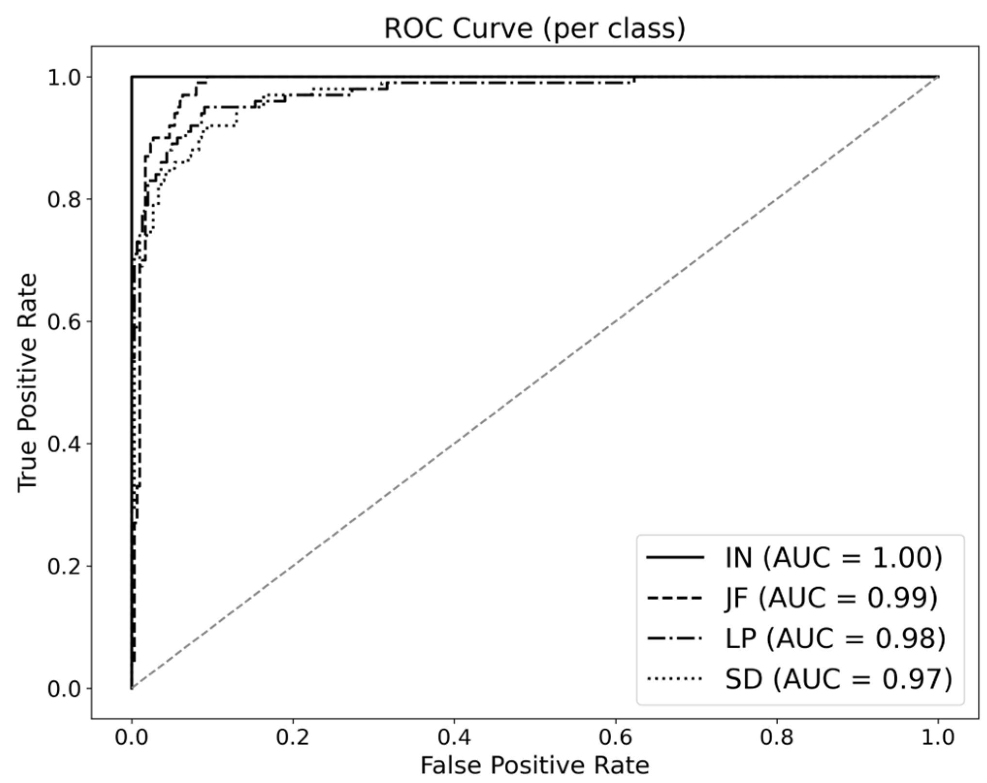
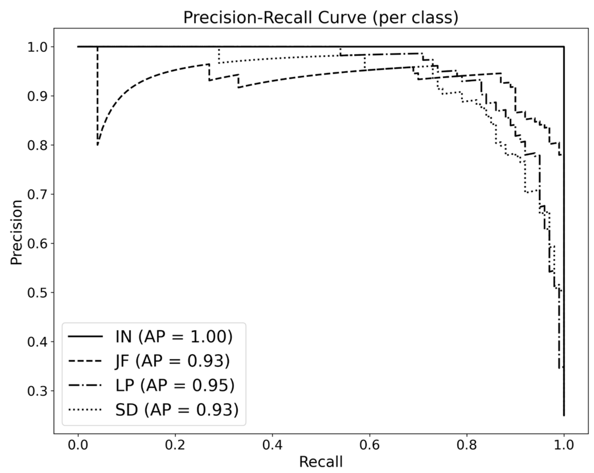
Figure 6 presents the ROC curves for each class, with AUC scores of 1.00 for IN, 0.99 for JF, 0.98 for LP, and 0.97 for SD, indicating that the model effectively distinguishes between classes. In addition, Figure 7 displays the PR curves, where the AP values were 1.00 for IN, 0.93 for JF, 0.95 for LP, and 0.93 for SD. These results demonstrate that the model maintains stable and reliable classification performance across all classes, even under data imbalance conditions, as reflected in consistently high AP values.

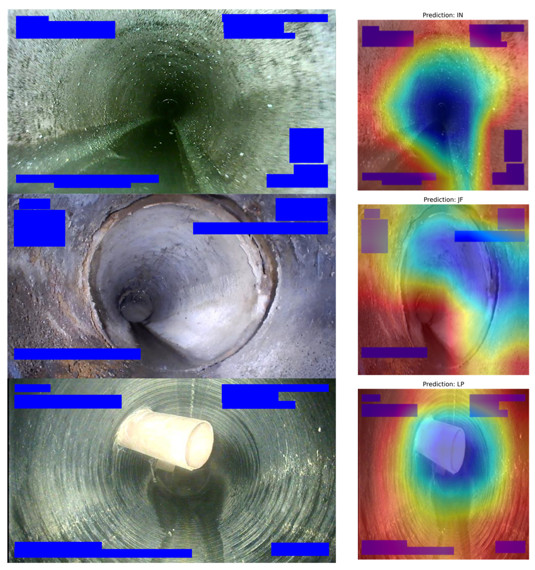
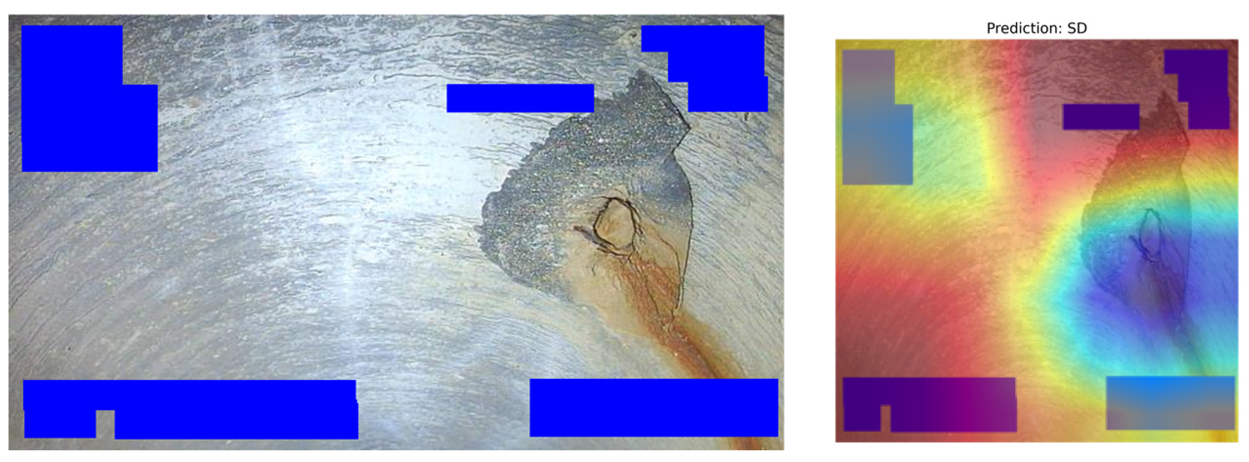
To visually analyze the basis of the model’s predictions, Grad-CAM was applied to test images to generate visual explanations. Grad-CAM (Gradient-weighted Class Activation Mapping) is a technique that highlights the regions of an input image where the model focuses when making a prediction, by producing a heatmap of the most salient features [40].

Figure 8 presents an input image (left) alongside its corresponding Grad-CAM visualization (right). In the heatmap, blue regions indicate areas where the model concentrated its attention, while red regions represent areas of lower relevance. The visualization confirms that the model focused on the actual defect areas, suggesting that it successfully learned meaningful visual features relevant to the classification task.

While the overall quantitative evaluation results support the strong performance of the model, misclassification may still occur in certain classes due to complex factors such as multiple overlapping defects. Accordingly, the following section provides an analysis of misclassified images to examine the model’s limitations and further investigates the impact of low-quality images present in the training dataset on model performance.

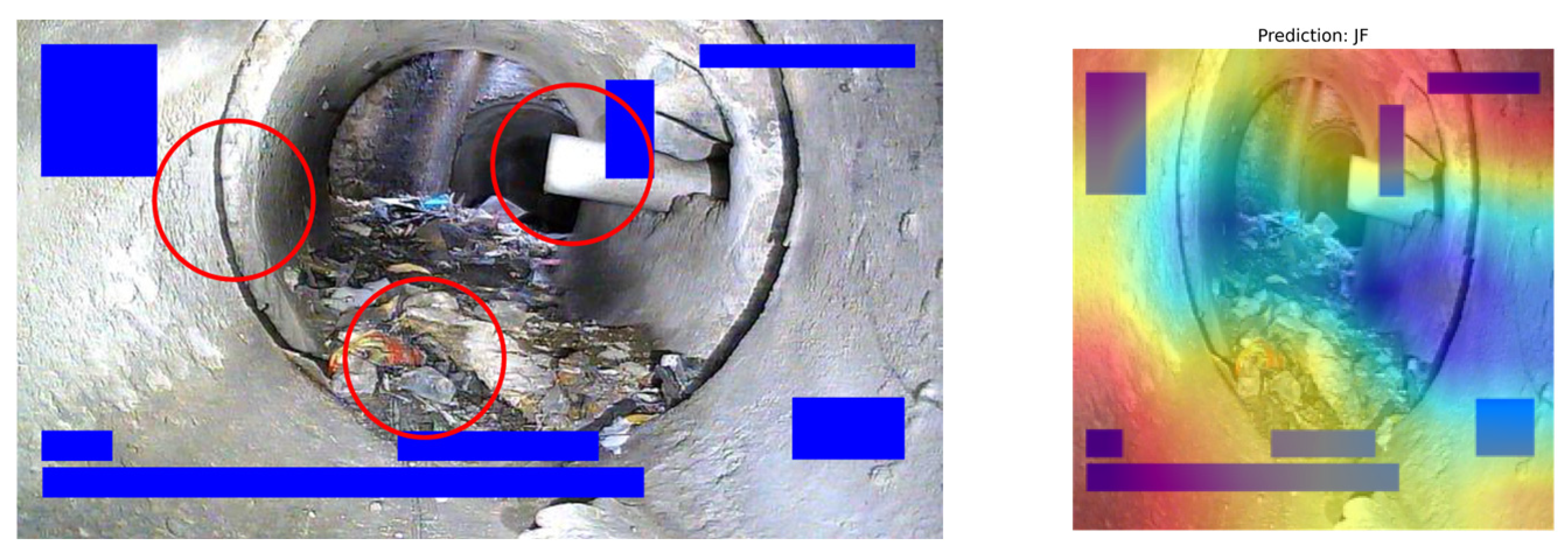
As shown in Figure 9, the model failed to correctly classify an image that simultaneously contains a lateral protrusion (LP) and a joint failure (JF). Although the image was originally labeled as LP, the model misclassified it as JF. As illustrated by the Grad-CAM visualization in Figure 9, the presence of multiple defects appears to have confused the model, leading it to focus on incorrect features during prediction.

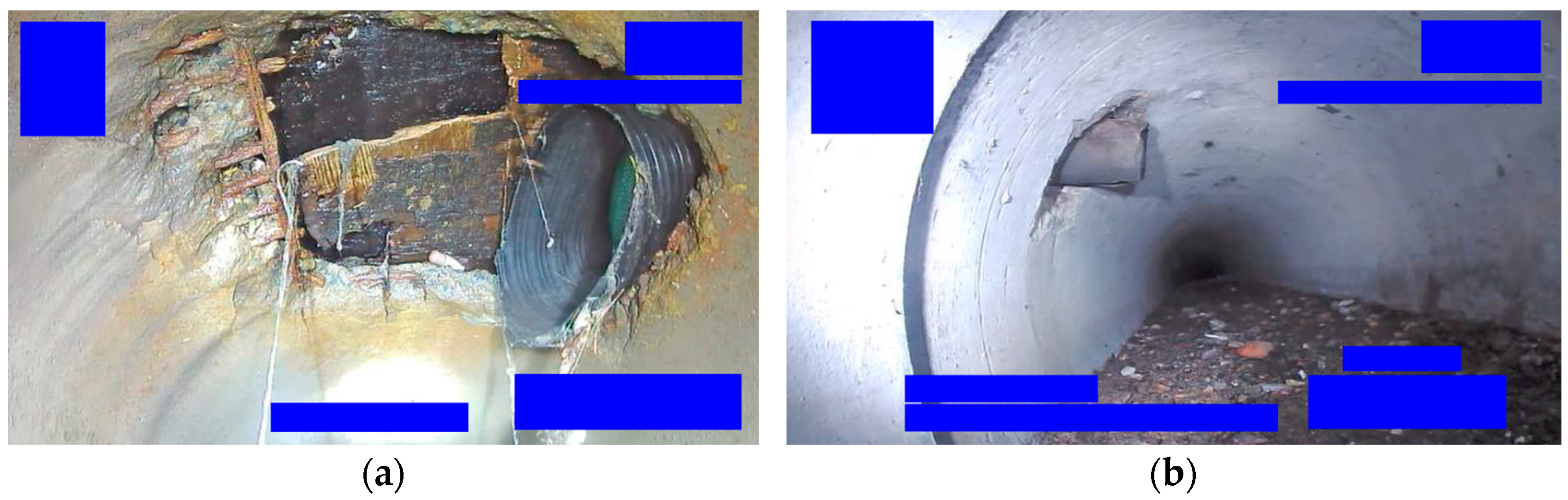
In addition to images containing multiple defects, some images may appear to be of low quality due to motion blur or occlusion of key defect features. However, such criteria are inherently subjective and difficult to quantify consistently. To establish a more objective and quantifiable definition of low-quality data, this study defines low-quality images as those containing two or more defect types within a single frame. Based on this criterion, additional experiments were conducted. Examples of such low-quality images are presented in Figure 10. To assess the defect rate of the training dataset, 4000 images (Set 1) were reviewed, revealing 102 mislabeled or duplicate defect images. The inclusion of these low-quality data in the training process likely contributed to limitations in the model’s accuracy improvement.

An experiment was conducted to analyze the impact of low-quality images in the training dataset on model accuracy (

Table 4. Mean and standard deviation of train dataset statistics.

Dataset	Normal Image	Low-Quality Image	Low-Quality Rate (%)	Accuracy (%)
Set 1-A	3898	0	0	72.50
Set 1	3898	102	2.5	69.00
Set 1-B	3750	250	6.25	62.25

). Set 1-A consisted of 3898 images, from which 102 identified low-quality images were removed. Set 1-B, on the other hand, was constructed by artificially increasing the number of low-quality images to 250, using additional mislabeled or flawed data from the full dataset.

The training results showed that Set 1-A achieved a 3.5% increase in accuracy compared to the original Set 1, which included low-quality images. The removal of duplicated defect images, censored images, and other low-quality data likely helped the model learn clearer defect patterns, thereby improving classification performance. In contrast, Set 1-B demonstrated a 6.75% decrease in accuracy as the number of low-quality images increased. This suggests that the presence of additional mislabeled data led to greater confusion in identifying defect types, ultimately degrading model performance.

3.4. Model Application

The sewer defect classification model developed in this study can serve as an automated diagnostic tool for practical integration into real-world sewer inspection systems. The deployment of the model in operational settings would involve the following steps:

First, during the data acquisition phase, internal video footage of sewer pipelines is captured using CCTV-equipped drones. Still images are extracted from the footage to serve as the foundational input data that visually represent the condition of the pipe interior.

Second, in the image preprocessing phase, the extracted images are resized and formatted to be compatible with the model’s input specifications.

Third, in the model inference phase, the preprocessed images are fed into the trained model, which classifies each image into one of four categories: intact (IN), joint failure (JF), lateral protrusion (LP), and surface damage (SD). The model outputs the class with the highest predicted probability as the final classification result.

Fourth, during the result interpretation and reporting phase, the classification outcomes are temporally reorganized to detect recurring defect patterns. A diagnostic report is generated, summarizing defect locations, types, and frequencies. This report can subsequently support maintenance prioritization and decision-making processes.

This end-to-end application workflow eliminates the subjectivity of manual inspections and significantly enhances the objectivity and efficiency of sewer condition assessments.

4. Conclusions

In this study, a CNN-based automated defect classification model was proposed using image data provided by AI-Hub, aiming to overcome the limitations of conventional sewer pipeline defect detection methods. The experimental results demonstrated that adjusting dropout rates and L2 regularization coefficients led to some improvement in classification accuracy.

Analysis of misclassified images from the final model revealed instances of mislabeling and multiple overlapping defects. These types of low-quality images were also found in the training dataset, which likely contributed to decreased model accuracy. Comparative analysis showed that as the proportion of low-quality data increased, model accuracy declined. While training with large datasets can improve performance up to a certain level, achieving higher model accuracy requires not only a sufficient volume of data but also high data quality.

Datasets contaminated with mislabeled or poor-quality images are difficult to correct due to their large size. Therefore, removing low-quality data from the initial dataset construction phase is essential for building a reliable dataset for future training. To ensure high-quality dataset development, image collection and labeling should involve validation by sewer inspection experts. Incorporating sufficient quantities of verified data into model training is expected to further enhance the accuracy of defect detection.

The technology for detecting sewer pipeline damage using artificial intelligence models should continue to evolve through ongoing research and development to meet future challenges and demands. The single-image-based classification approach lacks temporal and spatial context, which can lead to misclassification in cases involving multiple overlapping defects or ambiguous defect boundaries. Moreover, the ResNet50-based static classification model has limited capacity to capture and incorporate detailed information about the location and morphology of defects. To address these limitations, future work may consider incorporating video-based models that leverage temporal information or applying end-to-end object detection frameworks capable of localizing and classifying defects simultaneously. In addition, the use of explainable AI (XAI) techniques—such as Grad-CAM—can enhance interpretability and trustworthiness by visualizing the model’s decision-making process.