What Are the Key Factors Influencing the Water Price in Interbasin Water Transfer Projects? An Integrated Fuzzy Decision-Making Trial and Evaluation Laboratory (DEMATEL)–Interpretive Structural Model (ISM)–Grey Relational Analysis (GRA) Method

Abstract

A reasonable water price for interbasin water transfer projects (IWTPs) is vital for solving the problem of unequal water use among different water users caused by different water source supply prices, promoting external water transfer consumption, and ensuring the stable and equitable project operation. However, the formulation of the water price is influenced by many factors, and it is necessary to identify the key factors and their interactions in the water prices formulation for IWTPs. In this study, we identified 15 factors that affect it. This paper used the fuzzy decision-making trial and evaluation laboratory (DEMATEL) to analyze the causal relationships and importance levels among the influencing factors. A four-level hierarchical structural model was established using an interpretive structural model (ISM), which intuitively displayed the hierarchical structure and pathways of each factor. The role of each influencing factor was determined by using MICMAC. Finally, the grey relational analysis method was used to identify the top five key factors: the socioeconomic development level, diversification of water resources, water demand of water users, cost of the project’s water supply, and national policies and regulations. Strategies to improve the formulation of water prices have also been proposed. The results show that the top five factors influencing the water price for IWTPs are the socio-economic development level, diversification of water resources, water demand of water users, cost of the project’s water supply, and national policies and regulations. The water price should be formulated based on the water resource cost, supply–demand relationships of water resources, and policy objectives to ensure scientific and reasonable cost allocation and differentiated pricing. For water-transfer projects with strong public welfare, the government may lower water prices through financial subsidies to alleviate the burden on water users.

1. Introduction

Owing to the impacts of population growth, economic development, improvements in living standards, and changes in consumption patterns, the severity of the conflict between regional water supply and demand is increasing. Water scarcity has become a common problem in many regions worldwide, with approximately 25% of major cities experiencing varying degrees of water scarcity [1,2]. The World Bank predicted that water demand in urban areas would increase by 50–70% over the next 30 years [3]. As an important project that benefits a country and its people, the construction and operation of IWTPs have become important for alleviating water supply–demand imbalance and promoting the coordinated development of regional water resources. Currently, there are over 350 water transfer projects in more than 40 countries, including the Central Valley Project in the United States, the Snow Mountain Water Transfer Project in Australia, the Indian River Interconnection Project, and the South-to-North Water Transfer Project in China [4,5,6,7,8]. Their implementation has eased water shortages along their routes and disrupted the spatial distribution structure of natural water resources [9]. The water prices formulation is a core aspect of water resource management in IWTPs. Scientific and reasonable water price formulation is vital for solving the problem of unequal water use among different water users caused by differences in water source prices, promoting the consumption of external water transfer, comprehensively considering the affordability of different water users, achieving “Pareto optimality” in the rights and interests of water-supply management departments, water-supply operators, and water users, and ensuring the stable and equitable operation of the project. Many countries have introduced multiple policies and proposed relevant requirements for the formulation of water prices in IWTPs. However, owing to long-term resource and water quality shortages, the value of water resources is continuously increasing, and the water collection rate in some areas is low. In addition, the diversification of investment entities and the complexity of property rights relationships in IWTPs often lead to phenomena such as “different prices for the same channel” and “different prices for the same source” during actual operations, resulting in a certain degree of difference in the water collection rate and benefit distribution between water users and water-supplying enterprises in water-receiving areas, as well as between different water-supplying enterprises. There is an urgent need to establish a balanced water price system to better reflect the changes in regional socioeconomic development and water resource conditions.

Current research on IWTPs has focused on the implementation status of such projects worldwide; water resource allocation between different watersheds; assessment of the impact of such projects on the environment, social economy, and water quality; the role of policies, regulations, and project sustainability in interbasin water transfer resource management; methods for determining the amount and price of interbasin water transfer; multidisciplinary evaluations of IWTPs; and research and development of water supply and distribution models [10,11,12]. However, there is a lack of research on the factors affecting water prices in IWTPs. Therefore, the following three questions must be answered: What factors affect the pricing of IWTPs? What are the interrelationships among the various factors and the extent to which they affect water prices? Finally, which factors play a crucial role in water pricing? The characteristics and main applications of existing influencing factor analysis methods are summarized in

Table 1. Analysis methods for influencing factors.

Method	Characteristics	Application
DEMATEL [13,14,15,16,17]	Assessment of causality and degree of influence between factors	Project construction risk, emergency decision-making, cost control, carbon footprint
MICMAC [18,19,20]	Categorizes the attributes and determines the role and status of influencing factors	Photovoltaic green roofs, organizational resilience of projects
ISM [21,22,23,24,25]	Delineates the system hierarchy and qualitatively analyzes the influencing relationship between each factor	Internet-based recycling by urban residents, cost control, high-quality development of green building, barriers to BIM implementation
ANP [20]	Determines the overall weighting of the factors	Photovoltaic green roofs
SD [26,27,28,29,30,31]	Explores the intrinsic connection between the influencing factors through quantitative methods	BIM application barriers, BIM adoption under government subsidy
SEM–SD [32]	Probes the mechanisms underpinning influencing factors, assesses the gradation of influence on objects, and executes a sensitivity simulation analysis	Prefabricated building supply chain
Structural Equation [31,32]	Allows for the analysis of the direct and indirect impacts of latent constructs between exogenous and endogenous variables	Performance of infrastructure projects
Fuzzy DEMATEL–ISM [18,33]	Allows for the analysis of the interrelationships, hierarchical structure, and mechanisms of factors, and addresses the shortcomings in semantic ambiguity	Organizational resilience of projects, photovoltaic green roofs
Dual-Drive DEMATEL [16]	Avoids the disadvantages of DEMATEL method relying on subjective experience calculation	Emergency decision-making
DEMATEL–ISM–MICMAC [14]	Determines the role of factors and clarifies their position in complex systems by calculating the driving force and dependence	Carbon footprint, high-quality development of green buildings
MLRM, RBDSS [34]	—	Implementation of photovoltaic power generation projects
BP-WINGS [35]	—	Green building development

.

The novelty and contributions of this study are as follows. First, this study systematically identified the factors affecting the water prices of IWTPs, which helps to achieve more scientific water price formulation. Second, we determined the significance of the factors and quantified the causal relationships between these factors to determine the causal and resulting factors for the water price of IWTPs using the DEMATEL method and established a multilevel recursive outcome model through the ISM method, which contributes to investigating the causal relationships and hierarchical structures of these driving forces and to determining the mechanisms of their interactions. Subsequently, autonomous, dependent, connected, and independent factors clarify the substantive roles of the factors in the system using the MICMAC model, o revealing the complex mechanisms of action between the factors. Finally, the GRA method was used to identify the key factors affecting the water prices of IWTPs. The combination of the four methods can provide a deeper understanding of the factors affecting water prices in IWTPs and the interaction mechanisms between them, which is helpful for the formulation of fairer and more reasonable water prices.

The remainder of this paper is organized as follows. Section 2 explains the research process, and Section 3 presents the research findings and analyses. A comprehensive analysis and discussion are presented in Section 4. Section 5 presents the conclusions and future prospects of this study.

2. Methodology

2.1. Establishment of the Influencing Factor System

Many stakeholders are involved in the formulation of water prices for IWTPs. Therefore, analysis of the influencing factors involves comprehensive and complex system engineering. Although little direct research has been conducted domestically and internationally on this topic, we can still use the Web of Science to identify various factors from the relevant literature based on keywords such as “water price”, “water supply price”, “IWTPs”, and “influence factors”. Initially, 22 factors were compiled and summarized. Then, the factors with weak influence were eliminated by the difference ranking and expert review methods, and 15 critical factors were selected and divided into four categories: socioeconomic, political system, natural environment, and engineering itself, as shown in

Table 2. Influencing factor indicators.

Dimension	Number	Critical Factors	Related Literature
Socio-economic factors	A1	Socio-economic development level	[36,37]
	A2	Regional industrial structure	[38]
	A3	Water demand of water users	[39,40]
	A4	Affordability to water users	[41]
Political system factors	A5	National policies and regulations	[42,43]
	A6	Government subsidies and incentives	[44]
	A7	Institutional and market factors	[45]
Natural environment factors	A8	Water resources’ quality	[44]
	A9	Diversification of water resources	[46]
	A10	Water resource abundance and scarcity	[47]
	A11	Water availability	[48]
Engineering factors	A12	Cost of project’s water supply	[49,50]
	A13	Guaranteed water supply rate	[51]
	A14	Project investment structure	[52]
	A15	Project profitability	[53]

.

2.1.1. Socio-Economic Factors

The main socioeconomic factors affecting the price of water supply include the level of economic development, regional industrial structure, demand of water users, and affordability to water users. (1) Socio-economic development level. Socioeconomic development is accompanied by high consumption of water resources, and complex economic activities bring about a series of problems, such as water pollution and functional decline. In regions with a higher level of socioeconomic development, the affordability to water users is relatively strong, and the water supply price can be higher; conversely, in regions with a lower level of socioeconomic development, the water supply price should be lower. (2) Regional industrial structure. The regional industrial structure and the water resources supply–demand relationship are indirectly positively correlated; therefore, the price of the water supply must not be high. If the proportion of high-tech industry is larger, the water supply price affordability is stronger, and the water supply price can be increased appropriately. (3) Demand of water users. The price of water from IWTPs is generally higher than that from local water sources. When their water demand is affected by the socioeconomic development level, water resource conditions, industrial structure, and other factors, and local water sources cannot meet their needs, they will consider external water transfer. Simultaneously, in an interbasin water transfer system, the higher the water supply volume, the lower the water supply cost per unit of water and the lower the water supply price. (4) Affordability to water users. Different water users have different water demand levels, and there are some differences in the affordability of water prices, even for the same type of water user, partly due to the differences in the effects of water use, mode, income level, dependence on water resources, etc., on water supply price affordability. Generally, the higher the affordability to water users, the higher the water supply price, and vice versa, the lower the water supply price.

2.1.2. Political System Factors

Policy and institutional factors, including national policies and regulations, government subsidies and incentive systems, and institutional and market factors, have direct or indirect impacts on the development of water supply prices, with strong unpredictability and mandatory effects. (1) National policies and regulations. National policies and regulations for IWTP water supply price development have a strong basis and play an important role in safeguarding. National policies and regulations affect the current period of water supply pricing behavior and the implementation of programs to regulate the price of water supply as much as possible to promote the reform of water supply price, and thus ensure the scientific and reasonable development of pricing. (2) Government subsidies and incentive system. To achieve the goals of guaranteeing the rights of water users in the receiving areas, governments often consider the economic status of water users, their water demand, and the regional investment environment. The formulation of water supply prices integrates water supply subsidies, incentives, and other control measures, as well as a series of preferential policies adopted by the state in the investment and financing of IWTPs and loans, which indirectly influence the price of water supply and lead to a reduction in water supply prices. (3) Institutional and market factors. Defects in the management system and operating mechanisms cause the price of the water supply and its actual value to deviate, resulting in water supply price distortion. With the deepening of the reform of the water supply price management system, the state has encouraged water users to develop and utilize water resources in accordance with the law. Therefore, the establishment of a complete information-sharing mechanism, open trading, fair competition, a relatively well-developed water resources trading market, the formation of stakeholder interests, and common public supervision of water resources are conducive to the rational formulation of water prices.

2.1.3. Natural Environment Factors

Natural factors are among the most important determinants of water supply pricing and determine the quantity and quality of regional water resources. Natural factors affecting the price of water supply in IWTPs include the quality of water resources, diversity of water resources, degree of water resource abundance and scarcity, and the amount of water resources available. (1) Water resource quality. Water resources are priced according to their quality, with low prices for high quantities and high prices for high quality. In the process of transferring water from IWTPs, there are two types of water resources of good quality: one is good in itself, and the other becomes good after a series of purification processes, which increases the cost of water purification, the latter of which is higher than the former. If the quality of water resources is low, the corresponding cost of the water supply is also lower. (2) Water resource diversification. Regional surface water, groundwater, water transfer, and other water resources entail different costs, which result in differences in the water prices, indirectly affecting the total regional water prices. Currently, in areas with external water diversion, in terms of engineering water prices, a significant amount of operating costs is consumed during the processes of water transmission and distribution, which are higher than the cost of local water sources. (3) Water resource abundance and scarcity. A shortage of resources will increase the opportunity cost of their use, as well as that of water resources. Water resource scarcity leads to interregional and seasonal price differences; therefore, the water supply pricing process should adequately measure the degree of scarcity of water resources. The price of water varies among regions with different levels of water scarcity. The water supply price in the same region also varies with seasonal changes in abundance and dryness. (4) Availability of water resources. Water resource conditions in different regions determine their scarcity. In regions with abundant water resources where IWTPs are implemented, the supply–demand imbalance among water users tends to be relatively minor, resulting in correspondingly lower water prices. Conversely, in water-scarce regions, the implementation of IWTPs typically leads to an increase in water pricing due to greater supply–demand pressures.

2.1.4. Engineering Factors

The IWTPs’ condition affects the cost of the project’s water supply by influencing the quality of operation and maintenance management, and it ultimately affects the water supply price. From the perspective of the project itself, the factors affecting the price of water supply mainly include the project water-supply cost, project water-supply guarantee rate, project investment structure, and project profitability. (1) Project’s water supply cost. It is the key element affecting the water supply price, and high and low values will directly affect the water price in IWTPs. The cost of the project’s water supply covers various expenses such as water resource acquisition, treatment, transportation, and facility maintenance. If the project is large in scale, or the water resource is remote and the water quality is complex, requiring deep treatment, the cost of the project’s water supply will increase. To ensure the normal operation and sustainable development of water supply enterprises, water prices will inevitably rise. (2) Project water-supply guarantee rate. The water-supply guarantee rate is a reflection of the degree of assurance of water supply projects, and high and low values reflect the quality and level of water supply services, with the water supply price being positively proportional. If the water-supply guarantee rate is high, the water supply unit provides higher quality and level of service, so the water supply service compensation is correspondingly high, increasing the project’s water supply costs, resulting in higher water supply prices. (3) Project investment structure. The IWTP investment structure determines the nature of the type of water supply, and different project investment structures require different rates of return on investment, which are indirectly caused by differences in the water supply price. (4) Project profitability. Project profitability is generally based on project costs and is the sum of profits and taxes. However, water pricing exhibits significant differences attributable to the water supply industry’s inherent monopoly, divergent regional policies, heterogeneous end-user categories, diverse water resource utilization patterns, and differential profitability profiles.

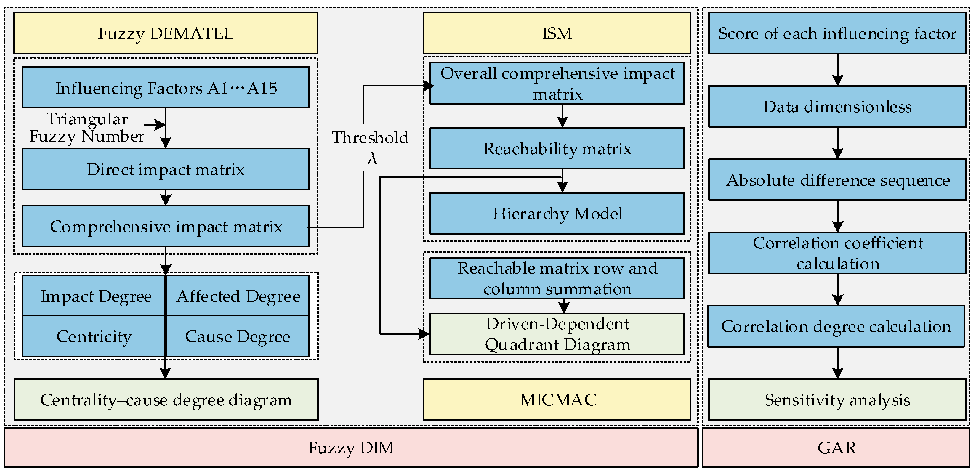
2.2. Research Framework

DEMATEL is a factor analysis method based on matrix tools and graph theory [54,55]. By measuring indicators, such as the degrees of impact, influence, cause, and centrality, the influence relationship, attributes, importance, and the logical relationship of the influencing factors of complex systems are quantitatively presented, which simplifies complex problems. In addition, triangular fuzzy numbers were introduced to transform expert semantics, and defuzzification was performed using the Converting Fuzzy Numbers into Crisp Scores (CFCS) [56], which is used for deblurring to develop the fuzzy DEMATEL method to reduce the impact of the variability in the subjective judgments of the experts and the ambiguity of the interactions among the factors by using the DEMATEL method, which affects the research results. As the fuzzy DEMATEL method cannot discern the hierarchical structural relationships among the influencing factors, a fuzzy DEMATEL–ISM explanatory structure model was established on this basis. We can analyze the dichotomous relationship among multiple influencing factors in a complex system and to analyze the correlation among the factors by using ISM. Based on the hierarchical division of the influencing factors from the fuzzy DEMATEL–ISM, the MICMAC analysis method is used to classify the attributes by calculating the dependence and driving forces of the influencing factors, which is beneficial for the in-depth analysis of the status and function of the influencing factors. Then, the fuzzy DIM (DEMATEL–ISM–MICMAC) method was developed, which can reflect the causal relationship between each influencing factor, the hierarchical division, and the dependence and drive within the system, but the degree of correlation between the factors is still a key issue to be solved. Therefore, the GRA method is used to compute the main relationship between the target factor and corresponding factors in order to identify the factor that has the greatest degree of influence on the target factor, and the intrinsic interconnection between the factors and their counterparts can be quantified by quantifying the relationship between them [57].

Therefore, the integration of the DIM and GRA methods in this study allows for the interrelationships among the restrictive factors for the water price of IWTPs to be systematically described so that a hierarchical structural model for the water price of IWTPs can be established and the correlation between each factor can be determined. A flowchart of this process is shown in Figure 1.

2.3. Research Methods

2.3.1. Fuzzy DIM Model

The combination of the fuzzy DEMATEL method, ISM, and MICMAC as a multi-criteria decision analysis method can allow the key influencing factors and their degree of influence in the formulation of the water price of IWTPs to be effectively identified, and the hierarchical division between various factors can be clarified, demonstrating their logical relationships. The steps were as follows:

Step 1: Establish a set of influencing factors A = {A₁, A₂, …, A_n}. The degree of influence between influencing factors was divided into five levels: very significant impact (4), high impact (3), certain impact (2), low impact (1), and no impact (0).

Step 2: Invite experienced experts to assign values to the impact levels of the 15 influencing factors and then obtain the direct impact matrix C = |c_ij|_n×n, where c_ij represents the degree of influence of factor A_i on factor A_j.

Step 3: Convert the direct impact matrix C into triangular fuzzy numbers (TFN), as listed in

Table 3. Semantic transformation table.

Semantic Variables	TFN
No impact	(0, 0, 0.25)
Low impact	(0, 0.25, 0.5)
Has a certain impact	(0.25, 0.5, 0.7)
Has a high impact	(0.5, 0.75, 1)
Has a very significant impact	(0.75, 1, 1)

. The triangular fuzzy number can be represented as Equation (1), where l is the left value, that is, the conservative value; m is the median value, which is the closest value to reality; and r is the right-hand value, which is an optimistic value. The degree to which the k-th expert believes that influencing factor i affects influencing factor j can be obtained.

Step 4: The CFCS method was used to blur and obtain direct impact matrix Z. The steps were as follows:

(1) Standardize triangular fuzzy numbers.

$$\begin{array}{l}l{s}_{ij}^k=(l_{ij}^k-\min l_{ij}^k)/{\Delta }_{\min }^{\max }\\ m{s}_{ij}^k=(m_{ij}^k-\min m_{ij}^k)/{\Delta }_{\min }^{\max }\\ r{s}_{ij}^k=(r_{ij}^k-\min r_{ij}^k)/{\Delta }_{\min }^{\max }\end{array}$$

(1)

where $l{s}_{ij}^k$, $m{s}_{ij}^k$, and $r{s}_{ij}^k$ are the standardized values of the left-side $l_{ij}^k$, intermediate $m_{ij}^k$, and right-side values of the triangular fuzzy numbers, respectively; and ${\Delta }_{\min }^{\max }$ = $\max r_{ij}^k$ − $\min l_{ij}^k$ is the difference between the left and right values.

(2) Standardize the left and right values. $u_{ij}^k$ and $v_{ij}^k$ are the standardized left and right values, respectively.

$$\begin{array}{l}{u}_{\mathrm{ij}}^{\mathrm{k}}={\mathrm{ms}}_{ij}^k/(1+m{s}_{ij}^k-l{s}_{ij}^k)\\ v_{ij}^k=r{s}_{ij}^k/(1+r{s}_{ij}^k-m{s}_{ij}^k)\end{array}$$

(2)

(3) Calculate the clear values of $z_{ij}^k$.

$$z_{ij}^k=\min c_{ij}^k+{\Delta }_{\min }^{\max }[\min u_{ij}^k(1-u_{ij}^k)+v_{ij}^k{v}_{ij}^k]/[1-u_{ij}^k+v_{ij}^k]$$

(3)

(4) Calculate the average of the clear values and obtain the direct impact matrix, $Z=|z_{ij}{|}_{n\times n}$.

$$z_{ij}=(z_{ij}^1+z_{ij}^2\dots +z_{ij}^k)/k$$

(4)

Step 5: Standardize the direct impact matrix and obtain the matrix G.

$$\lambda =1/\underset{l\le i\le n}{\max }{\displaystyle \sum _{j=1}^n{z}_{ij}},G=\lambda Z$$

(5)

Step 6: Calculate the comprehensive impact matrix T.

$$T=G{(I-G)}^{-1}$$

(6)

Step 7: Calculate the impact degree and affected degree.

$$\begin{array}{l}{f}_i={\displaystyle \sum _{j=1}^n{t}_{ij}},i=1,2,\dots n\\ e_i={\displaystyle \sum _{i=1}^n{t}_{ij}},j=1,2,\dots n\end{array}$$

(7)

where t_ij is the impact value of the i-th element on the j-th factor in the comprehensive impact matrix T; f_i is the impact degree of factor i; and e_i is the affected degree of factor i.

Step 8: Calculate centrality and causality.

$$\begin{array}{l}{M}_i=f_i+e_i,i=1,2,\dots n\\ N_i=f_i-e_i,i=1,2,\dots n\end{array}$$

(8)

Step 9: Calculate the overall impact matrix H.

$$H=T+I$$

(9)

Step 10: Calculate the reachability matrix K.

$$k_{ij}=\left\{\begin{array}{l}1,h_{ij}\ge \lambda \\ 0,h_{ij}>\lambda \end{array}\right.(i,j=1,2,\dots n),K={[k_{ij}]}_{n\times n}$$

(10)

where λ is the threshold, λ ∈ [0, 1]; the larger the value of λ, the more significant the simplification effect on the structure. In practical analysis, it is necessary to determine the value of λ based on the system complexity. k_ij is the correlation between the factors i and j.

Step 11: Establish antecedent and reachable sets.

$$\begin{array}{l}A(s_i)=\{s_j\in S|k_{ij}=1\}\\ R(s_i)=\{s_j\in S|k_{ij}=1\}\end{array}$$

(11)

where A(s_i) is the antecedent set, which is the set of factors corresponding to rows s_i where all the factors in a column of a reachable matrix are 1. R(s_i) is the reachable set and the set of factors corresponding to column s_i in a reachable matrix, where all factors in the row are 1. When a certain factor a_i is satisfied R(a_i) = R(a_i) ∩ S(a_i), a_i is the factor at the highest level. Delete the rows and columns corresponding to factor a_i in the reachable matrix K; recalculate the reachable set, antecedent set, and intersection; and continue to search for the next layer until factor partitioning is completed, forming the final hierarchical partitioning result.

Step 12: With the MICMAC method, determine the dependencies and driving forces of the influencing factors based on the reachable matrix K.

$$\begin{array}{l}{D}_i={\displaystyle \sum _{j=1}^n{k}_{ij}}\\ R_i={\displaystyle \sum _{i=1}^n{k}_{ij}}\end{array}$$

(12)

where D_i is the driving force, and the R_i is dependence force.

Subsequently, a classification diagram of the influencing factors was drawn based on the results of the driving and dependence forces. The factors affecting the water price of IWTPs can be divided into self, independent, dependent, and linkage clusters based on the above analysis.

2.3.2. GRA Method

GRA is a dynamic statistical analysis method that can evaluate the sensitivity of various influencing factors and reflects the strength of the correlation between various factors by calculating and ranking the degree of correlation [58]. The steps were as follows:

Step 1: Determine the sequence matrix. The relational analysis determines the reference sequence X (related variables) and comparison sequence Y (stability coefficient). The average value of each factor affecting water prices in the IWTPs is used as a comparison sequence.

Step 2: Dimensionless data processing. Due to the inconsistent relative index data of various influencing factors, different dimensions, and significant differences in numerical values, it was not possible to directly compare them. Therefore, the original data are processed to render them dimensionless.

$$\begin{array}{l}{x}_{ij}^{\prime }={\displaystyle \frac{x_{ij}-\min x_{ij}}{\max x_{ij}-\min x_{ij}}}\\ y_{ij}^{\prime }={\displaystyle \frac{y_{ij}-\min y_{ij}}{\max y_{ij}-\min y_{ij}}}\end{array}$$

(13)

Step 3: Calculate the absolute difference between the indicator sequence and the corresponding elements of the evaluated object based on standardized data.

$$\left|x_0(k)-x_i(k)\right|(k=1,\dots ,n)$$

(14)

Step 4: Calculate the correlation coefficient.

$$\begin{gathered} {\zeta }_i(k)={\displaystyle \frac{{\min }_i{\min }_k\left|x_0(k)-x_i(k)\right|+\rho \cdot {\max }_i{\max }_k\left|x_0(k)-x_i(k)\right|}{\left|x_0(k)-x_i(k)\right|+\rho \cdot {\max }_i{\max }_k\left|x_0(k)-x_i(k)\right|}} \\ k=1,2,\dots ,m \end{gathered}$$

(15)

where ρ is the resolution coefficient, which belongs to (0, 1). Generally, ρ = 0.5.

Step 5: Calculate the degree of correlation. The 15 influencing factors are calculated separately and compared with the mean coefficients of the corresponding elements in the reference sequence to reflect the correlation between the main influencing factors and reference sequence.

$$r_{0i}={\displaystyle \frac{1}{m}}{\displaystyle \sum _{k=1}^m{\zeta }_i}(k), k=1,2,\dots \dots ,n$$

(16)

3. Results

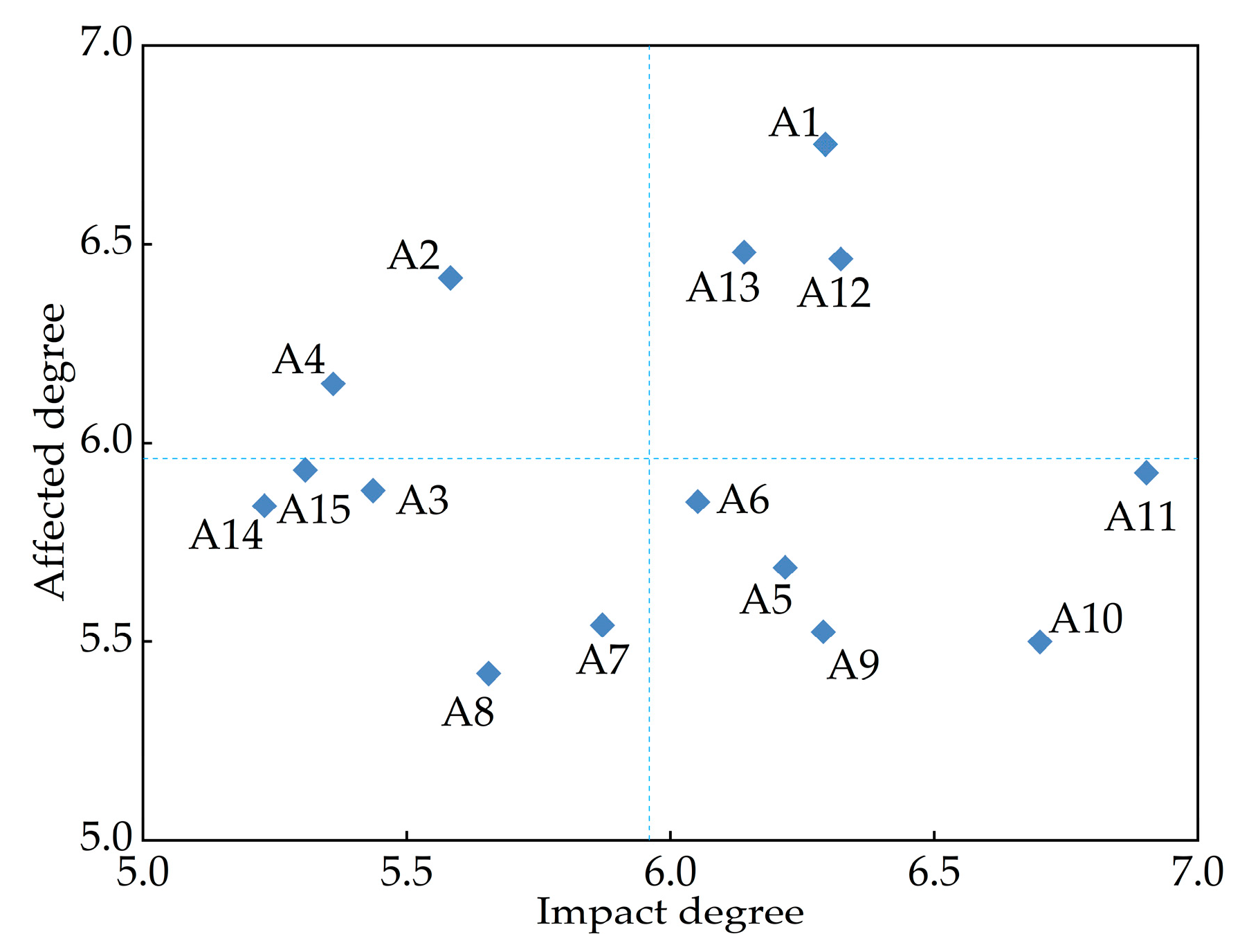
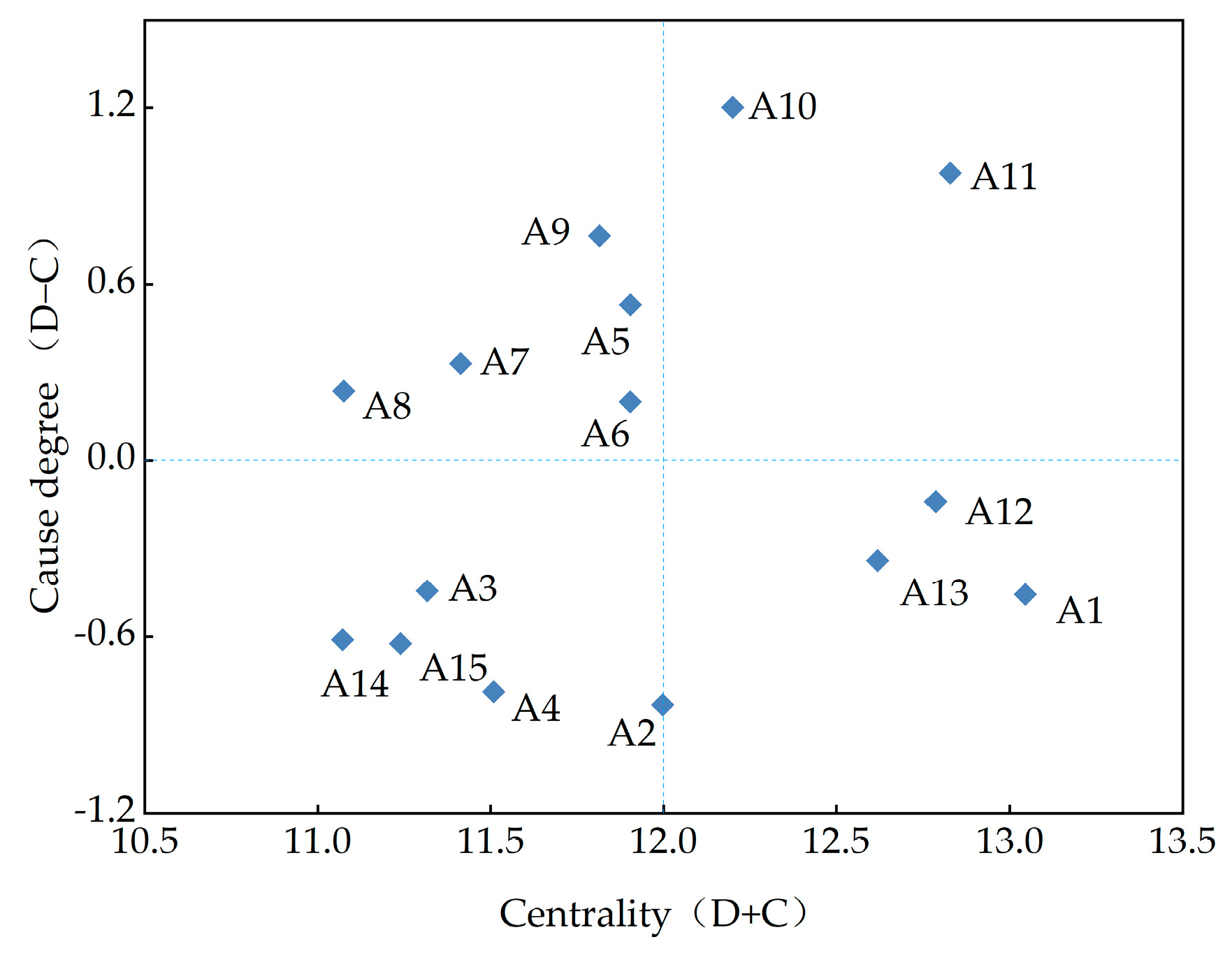
3.1. Fuzzy DIM Analysis

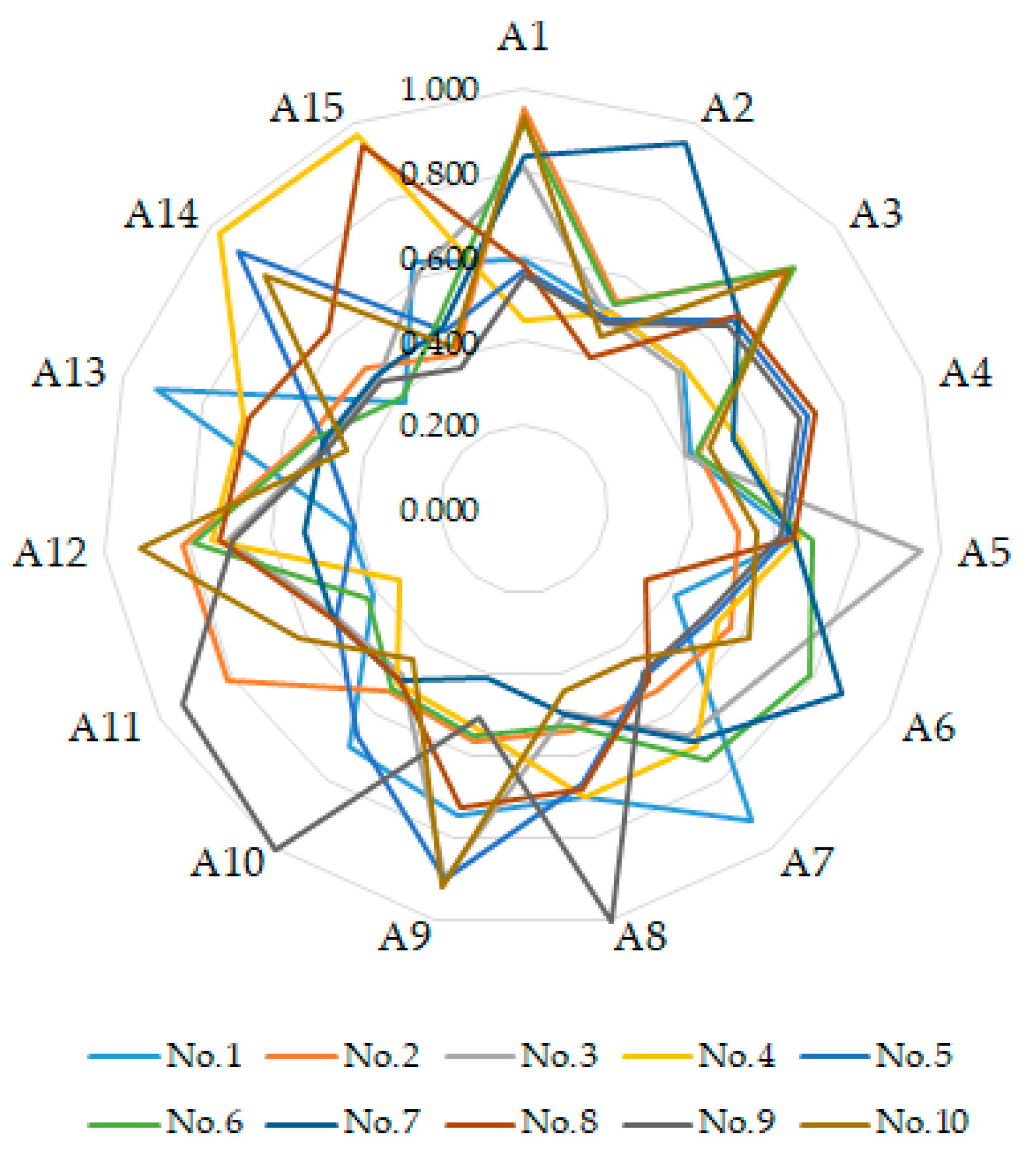
Some studies have found that when the number of experts involved in decision-making is between 5 and 10, the decisions made are more appropriate [59]. Based on this, eight experts with over five years of work experience, including two experts from the government, three experts from water transfer companies, and three representative water users, were invited to assign values to the impact levels among the 15 influencing factors. The results were then organized, summarized, and converted into triangular fuzzy numbers. The CFCS method was used to defuzzify the data and calculate the comprehensive impact matrix of the factors affecting the water price of IWTPs, as shown in

Table 4. Comprehensive impact matrix.

Factor	A1	A2	A3	A4	A5	A6	A7	A8	A9	A10	A11	A12	A13	A14	A15
A1	0.411	0.462	0.417	0.443	0.406	0.418	0.395	0.392	0.388	0.384	0.417	0.453	0.461	0.425	0.423
A2	0.437	0.347	0.370	0.384	0.369	0.369	0.359	0.353	0.355	0.349	0.372	0.394	0.395	0.365	0.365
A3	0.410	0.392	0.310	0.386	0.351	0.355	0.331	0.337	0.341	0.342	0.366	0.402	0.401	0.350	0.364
A4	0.412	0.380	0.372	0.320	0.345	0.361	0.335	0.316	0.324	0.332	0.361	0.394	0.398	0.350	0.360
A5	0.480	0.453	0.405	0.422	0.343	0.424	0.406	0.376	0.389	0.378	0.413	0.446	0.454	0.414	0.416
A6	0.455	0.447	0.396	0.427	0.395	0.343	0.394	0.364	0.371	0.374	0.404	0.445	0.434	0.397	0.407
A7	0.463	0.441	0.379	0.402	0.385	0.395	0.316	0.353	0.361	0.357	0.391	0.431	0.422	0.392	0.385
A8	0.434	0.408	0.377	0.394	0.361	0.365	0.341	0.297	0.352	0.349	0.388	0.420	0.419	0.372	0.379
A9	0.480	0.448	0.411	0.432	0.408	0.414	0.387	0.395	0.337	0.407	0.433	0.465	0.459	0.406	0.409
A10	0.502	0.483	0.454	0.471	0.421	0.437	0.416	0.404	0.423	0.357	0.463	0.493	0.499	0.438	0.442
A11	0.525	0.502	0.472	0.483	0.437	0.448	0.429	0.419	0.431	0.446	0.396	0.501	0.509	0.447	0.458
A12	0.479	0.451	0.424	0.448	0.402	0.420	0.384	0.389	0.400	0.396	0.415	0.395	0.465	0.422	0.435
A13	0.470	0.443	0.418	0.429	0.392	0.407	0.384	0.372	0.387	0.376	0.404	0.446	0.385	0.409	0.419
A14	0.396	0.379	0.337	0.344	0.335	0.348	0.330	0.322	0.330	0.321	0.347	0.391	0.387	0.296	0.367
A15	0.399	0.379	0.337	0.365	0.337	0.350	0.337	0.333	0.336	0.332	0.356	0.389	0.392	0.360	0.305

.

In steps 7 and 8, Equations (7) and (8) are used to calculate the impact degree, affected degree, centrality, and causality of the factors affecting the water price of IWTPs, as shown in

Table 5. DEMATEL calculation index values.

Factor	Impact Degree		Affected Degree		Causal Degree		Centrality		Factor Attribute
	fi	Rank	ei	Rank	fi − ei	Rank	fi + ei	Rank
A1	6.3	4	6.8	1	−0.5	11	13.0	1	R
A2	5.6	11	6.4	4	−0.8	15	12.0	6	R
A3	5.4	12	5.9	8	−0.4	10	11.3	12	R
A4	5.4	13	6.1	5	−0.8	14	11.5	10	R
A5	6.2	6	5.7	11	0.5	4	11.9	7	C
A6	6.1	8	5.9	9	0.2	7	11.9	8	C
A7	5.9	9	5.5	12	0.3	5	11.4	11	C
A8	5.7	10	5.4	15	0.2	6	11.1	14	C
A9	6.3	5	5.5	13	0.8	3	11.8	9	C
A10	6.7	2	5.5	14	1.2	1	12.2	5	C
A11	6.9	1	5.9	7	1.0	2	12.8	2	C
A12	6.3	3	6.5	3	−0.1	8	12.8	3	R
A13	6.1	7	6.5	2	−0.3	9	12.6	4	R
A14	5.2	15	5.8	10	−0.6	12	11.1	15	R
A15	5.3	14	5.9	6	−0.6	13	11.2	13	R

Note: C represents the causal factor, and R represents the result factor.

.

The impact and affected degrees refer to the degrees to which an influencing factor affects and is influenced by other factors in the system. Centrality refers to the position and degree of influence of the influencing factors in the system, that is, the sum of the impact and affected degrees. The causal degree refers to the direct causal relationship between various factors, which is the difference between the impact and affected degrees. If the causal degree of a factor is positive, the factor attribute is the causal factor, which is usually an indirect factor affecting the water price; if it is negative, it is the result factor, which is direct. According to Table 5, seven causal factors and eight resulting factors constrain the water prices of IWTPs. Among them, the top five impact factors were A11, A10, A12, A1, and A9, with impact degrees of 6.9, 6.7, 6.3, 6.3, and 6.3, respectively, indicating that these five factors had the most significant impact on the other factors.

Based on the impact degree, affected degree, centrality, and causal degree, the causal relationship between the factors influencing the water price of the IWTPs was determined, as shown in Figure 2 and Figure 3.

Among the 15 influencing factors, the top 5 with the highest centralities were A1, A11, A12, A13, and A10, with values of 13.0, 12.8, 12.8, 12.6, and 12.2, respectively, indicating that they had the most significant impact on the water price of IWTPs. In this study, we simplified the system structure by setting a threshold of λ=0.4 on the basis of previous research to remove the influence relationship between factors with weak impact. Subsequently, the reachability matrix was obtained according to Steps 9 and 10, as listed in

Table 6. Reachability matrix.

Factor	A1	A2	A3	A4	A5	A6	A7	A8	A9	A10	A11	A12	A13	A14	A15
A1	1	1	0	1	0	0	0	0	0	0	0	1	1	0	0
A2	0	1	0	0	0	0	0	0	0	0	0	0	0	0	0
A3	0	0	1	0	0	0	0	0	0	0	0	0	0	0	0
A4	0	0	0	1	0	0	0	0	0	0	0	0	0	0	0
A5	1	1	0	0	1	0	0	0	0	0	0	1	1	0	0
A6	1	1	0	0	0	1	0	0	0	0	0	1	0	0	0
A7	1	0	0	0	0	0	1	0	0	0	0	0	0	0	0
A8	0	0	0	0	0	0	0	1	0	0	0	0	0	0	0
A9	1	1	0	0	0	0	0	0	1	0	0	1	1	0	0
A10	1	1	1	1	0	0	0	0	0	1	1	1	1	0	0
A11	1	1	1	1	0	1	0	0	0	1	1	1	1	1	1
A12	1	1	0	1	0	0	0	0	0	0	0	1	1	0	0
A13	1	0	0	0	0	0	0	0	0	0	0	1	1	0	0
A14	0	0	0	0	0	0	0	0	0	0	0	0	0	1	0
A15	0	0	0	0	0	0	0	0	0	0	0	0	0	0	1

.

The reachable set, antecedent set, and their intersection were determined using Equation (11) based on the reachability matrix.

Table 7. Reachable set, antecedent set, and their intersection.

Factor	Reachable Set	Antecedent Set	Intersection
A1	1, 2, 4, 12, 13	1, 5, 6, 7, 9, 10, 11, 12, 13	1, 12, 13
A2	2	1, 2, 5, 6, 9, 10, 11, 12	2
A3	3	3, 10, 11	3
A4	4	1, 4, 10, 11, 12	4
A5	1, 2, 5, 12, 13	5	5
A6	1, 2, 6, 12	6, 11	6
A7	1, 7	7	7
A8	8	8	8
A9	1, 2, 9, 12, 13	9	9
A10	1, 2, 3, 4, 10, 11, 12, 13	10, 11	10, 11
A11	1, 2, 3, 4, 6, 10, 11, 12, 13, 14, 15	10, 11	10, 11
A12	1, 2, 4, 12, 13	1, 5, 6, 9, 10, 11, 12, 13	1, 12, 13
A13	1, 12, 13	1, 5, 9, 10, 11, 12, 13	1, 12, 13
A14	14	11, 14	14
A15	15	11, 15	15

presents the results. Then, we divided the influencing factors into hierarchical levels as shown in

Table 8. Hierarchical division of influencing factors.

Level	Element Set	Impact Degree
L1	2, 3, 4, 8, 13, 14, 15	Surface level
L2	1, 12	Intermediate level
L3	5, 6, 7, 9, 10	Intermediate level
L4	11	Deep level

.

In addition, a system-directed graph (Figure 4) and a multilevel ISM (Figure 5) were drawn to illustrate the factors affecting the water prices of IWTPs based on the hierarchical division of the influencing factors. Figure 4 and Figure 5 illustrate the hierarchical arrangement and progressive sequence of factors, highlighting the importance of various influencing factors on the water prices of IWTPs. These factors can be classified into three levels: surface, intermediate, and deep. Among them, the surface-level factors are easily influenced by other factors, whereas the intermediate-level factors play a bridging role and are influenced by the deep layer and, in turn, affect surface-level factors. Within the model, the top layer comprises factors with a direct impact that exert the most direct influence on the water price of IWTPs and, in turn, are affected by other factors. The factors located at the bottom are fundamental influencing factors that play a decisive role in influencing all intermediate and surface factors, thereby causing overall changes. Figure 5 shows the four levels of the structure. Layer 1 consisted of the direct factors at the surface level and included A2, A3, A4, A8, A13, A14, and A15. Layers 2 and 3 are intermediate-level factors, including A1, A5, A6, A7, A9, A10, and A12. Layer 4 consists of deep-rooted influencing factors, including A11. When improving the pricing strategy for IWTPs, the direct factors must be gradually improved from the basic ones. As shown in Figure 5, water availability (A11), which belongs to the natural environment dimension, is a deep-rooted influencing factor. The availability of water resources may vary depending on regional differences and changes with seasons with higher abundance and scarcity. Water resources in a region generally include surface water, groundwater, and water from external transfer. The cost of obtaining different types of water resources varies, which in turn affects the overall water price in the region. Political system factors, partial natural environment factors, partial engineering factors, and socioeconomic development levels were considered intermediate-level factors. For example, the socioeconomic development level (A1) is influenced by water availability (A11) and is closely related to water resource abundance and scarcity (A10); the higher the socioeconomic development level (A1), the greater the affordability for water users (A4), and the water price can be higher, while in regions with lower socioeconomic development levels, the water price should be lower. The remaining factors are surface-level factors.

The MICMAC model can verify the driving relationships in the ISM, and the results of the MICMAC driving force–dependency matrix can be mutually confirmed with the factor hierarchy topology in the ISM, ensuring the consistency and accuracy of the results. Subsequently, the driving force and dependency value of each factor were calculated using Equation (12) in Step 12, as listed in

Table 9. Driving force and dependency values of each influencing factor.

Factor	Dependence	Driving Force	Factors	Dependence	Driving Force	Factors	Dependence	Driving Force
A1	9	5	A6	2	4	A11	2	11
A2	8	1	A7	1	2	A12	8	5
A3	3	1	A8	1	1	A13	7	3
A4	5	1	A9	1	5	A14	2	1
A5	1	5	A10	2	8	A15	2	1

, and a MICMAC analysis quadrant diagram was drawn, as shown in Figure 6. As shown in Figure 6, the average driving force and dependency values were used to determine the dividing line for dividing the diagram into four classifications: autonomous, dependent, contacted, and independent clusters. Factors A10 and A11 are independent factors generally located at the deep level of the ISM. This type of cluster has a strong driving force and weak dependence, which can have a significant impact on other factors and is the fundamental influencing factor. Factors A1, A2, A4, A12, and A13 are dependent factors generally located at the surface level of the ISM. This type of cluster has a weak driving force and strong dependence, connects strongly with other factors, and is easily influenced by other factors. The factors in the autonomous factor cluster had low dependence on driving forces, and their influence was not strong. They were generally located at the intermediate level in the hierarchical topology diagram and played a connecting role, and included A3, A5, A6, A7, A8, A9, A14, and A15. When the driving force and dependence of factors within an autonomous cluster are strong, close attention to them must be paid. The hierarchical division results of the ISM were validated using MICMAC, verifying the effectiveness of the correlation mechanism and the hierarchical relationship division of various factors related to the water prices of IWTPs.

3.2. GRA

Ten experts from relevant fields were invited to score the degree of correlation between the 15 factors affecting the water price of IWTPs. The selection of the reference sequence and the comparison sequence is directly related to the accuracy of the analysis results. The original sequence usually refers to the main sequence that reflects the behavioral characteristics of the system, while the comparative sequence refers to the sequence of possible factors that affect the system behavior. Therefore, the original data were used as the comparison sequence, and the average value was used as the reference sequence. There may be some data bias caused by the different scoring criteria of experts. Therefore, the data were processed to be dimensionless using Equation (13) and linearly mapped to [0, 1] through calculations to ensure fairness and consistency of the results. By comparing and analyzing the comparison and reference sequences more accurately using Equation (14), the correlation degree between the influencing factors and a suitable water price for IWTPs can be determined. Subsequently, the resolution coefficient ρ was set to 0.5 [60,61,62], and the correlation coefficient was calculated using Equation (15), as shown in

Table 10. Correlation coefficients.

No.	A1	A2	A3	A4	A5	A6	A7	A8	A9	A10	A11	A12	A13	A14	A15
1	0.590	0.510	0.510	0.416	0.652	0.416	0.918	0.701	0.747	0.701	0.416	0.416	0.918	0.381	0.641
2	0.949	0.539	0.836	0.435	0.515	0.567	0.539	0.539	0.567	0.539	0.812	0.812	0.539	0.503	0.397
3	0.812	0.492	0.492	0.404	0.949	0.710	0.668	0.492	0.903	0.492	0.515	0.710	0.492	0.462	0.613
4	0.449	0.510	0.510	0.534	0.660	0.534	0.701	0.701	0.534	0.510	0.340	0.747	0.701	0.974	0.974
5	0.567	0.492	0.668	0.710	0.630	0.515	0.492	0.668	0.903	0.668	0.515	0.404	0.492	0.911	0.462
6	0.918	0.529	0.861	0.428	0.692	0.789	0.738	0.529	0.555	0.529	0.428	0.789	0.529	0.391	0.494
7	0.836	0.948	0.684	0.524	0.645	0.875	0.684	0.501	0.410	0.501	0.524	0.524	0.501	0.470	0.470
8	0.578	0.395	0.684	0.728	0.645	0.336	0.501	0.684	0.728	0.501	0.524	0.728	0.684	0.627	0.941
9	0.555	0.484	0.652	0.692	0.616	0.505	0.484	1.000	0.505	1.000	0.933	0.692	0.484	0.454	0.366
10	0.933	0.445	0.849	0.464	0.555	0.616	0.445	0.445	0.918	0.445	0.616	0.918	0.445	0.830	0.420

and Figure 7.

The correlation degree between each influencing factor and the reference benchmark was determined according to the calculated correlation coefficients, as shown in

Table 11. Correlation degrees.

Factor	Correlation Degree	Rank	Factor	Correlation Degree	Rank	Factor	Correlation Degree	Rank
A1	0.719	1	A6	0.586	10	A11	0.562	13
A2	0.535	14	A7	0.617	7	A12	0.674	4
A3	0.675	3	A8	0.626	6	A13	0.579	11
A4	0.534	15	A9	0.677	2	A14	0.600	8
A5	0.656	5	A10	0.589	9	A15	0.578	12

and Figure 8. From the above results, the larger the correlation degree, the closer the correlation with the reference value and the higher the corresponding evaluation. Among the ten sets of data evaluated, the correlation degrees were distributed within the range of 0.534–0.719, indicating that these evaluation factors had a significant impact on the water price of IWTPs. Among them, A1 had the highest comprehensive evaluation, with a correlation degree of 0.719, indicating that this factor is crucial to the future water price of IWTPs. A high level of economic development can result in an increase in water demand; in economically advanced cities, population growth and industrial expansion continuously drive up water resource requirements, potentially leading to water scarcity and subsequently increasing water prices. To address the rising water demand, it may become necessary to explore new water sources and construct water supply infrastructure, which would escalate water supply costs and consequently impact water pricing. Simultaneously, with socio-economic progress, water users’ capacity to afford higher water prices also tends to increase. A9 was next, with a correlation coefficient of 0.677. It directly affects the water price structure mainly through the difference in water resource types, cost, quality, development conditions, and policy orientation. The degree of correlation of A4 was 0.534, although it ranked last, and the degree of correlation was still relatively high. In the process of water price formation, water users primarily function as recipients rather than decision-makers, exhibiting a relatively low correlation with other factors influencing water prices in IWTPs. This is mainly because water prices are more directly determined by factors such as water resource endowment, the cost of the project’s water supply, and policies and regulations. Water users typically lack the ability to directly influence water prices, and their water demand tends to be less sensitive to price changes.

4. Discussion

Combined with the analysis of the fuzzy DIM and GRA methods, we identified the top five crucial factors influencing the water price for IWTPs as the socioeconomic development level (A1), diversification of water resources (A9), demand of water users (A3), cost of the project’s water supply (A12), and national policies and regulations (A5).

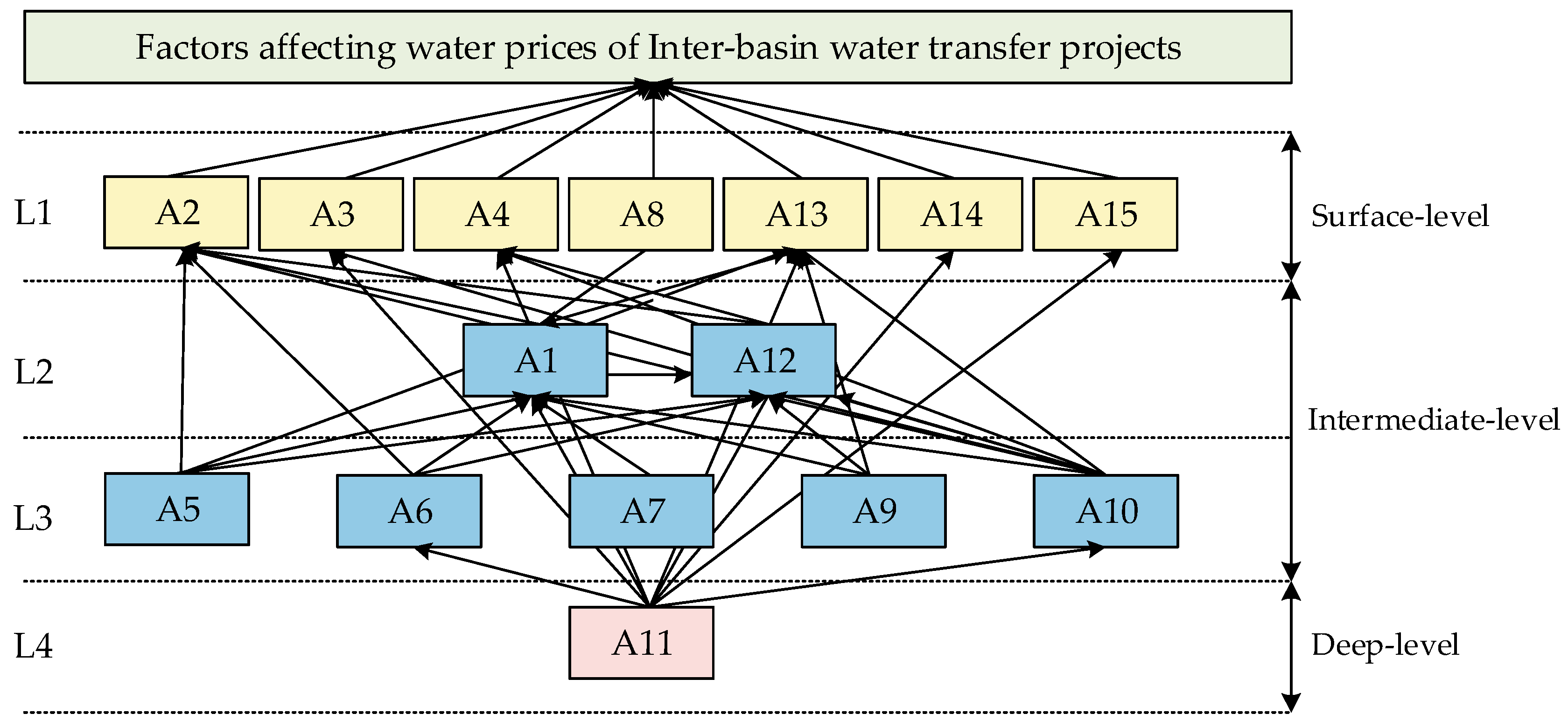
• The socioeconomic development level (A1) is a strong result factor, with the highest centrality and affected degree. It is also an intermediate-level factor that influences the water price of IWTPs and significantly affects other factors. The impact of the socioeconomic development level on the water price of IWTPs is mainly reflected in aspects such as the water supply cost, water demand, and payment capacity. Governments and enterprises in developed areas may be more willing to invest funds in constructing efficient water treatment facilities, water pipelines, and monitoring systems to improve water supply efficiency and quality. These inputs are reflected in the water price, resulting in relatively higher water prices. In areas with high water demand and widespread awareness of water-saving technologies among water users, water pricing focuses more on promoting water conservation through price leverage, such as by implementing tiered water pricing to encourage efficient water use. Water users have a strong ability to pay for water resources and can afford higher prices.
• The diversification of water resources (A9) is strongly influenced by natural environmental factors and ranks second in its degree of correlation. It is also an intermediate-level factor with a weak driving force and degree of dependence that influences the water prices of IWTPs. The impact of the diversification of water resources on the water prices of IWTPs is mainly reflected in multiple aspects. For example, the diversification of water resources provides more options for IWTPs but also increases the complexity of water pricing. The supply and demand relationships must be balanced through a water pricing mechanism. If there are local water sources or other water diversion projects in the area, IWTPs need to be reasonably priced and compete with alternative water sources to avoid water resource waste caused by oversupply. Diversified water resources can alleviate seasonal water shortages to some extent; however, measures should be taken to reduce prices during the wet season and increase prices during the dry season to ensure the basic benefits of the project. Therefore, the water price should be formulated based on the water source cost, supply–demand relationship of water resources, and policy objectives to ensure scientific and reasonable cost allocation and differentiated pricing.
• The demand of water users (A3) is one of the key influencing factors for the pricing of IWTPs and is a result of socioeconomic factors, which are surface-level factors affecting water prices. Water demand can be divided into rigid and elastic demands. Rigid demand is less sensitive to water prices and is the bottom line of the water price formulation. As a basic livelihood requirement, water prices must cover the water supply cost and ensure affordability for low-income groups. Elastic demand is highly sensitive to water prices, such as major water-consuming industries that are sensitive to water prices. Reasonable pricing can force enterprises to upgrade their water-saving technologies. Agriculture is a major water user; however, farmers have a poor ability to afford water. Water conservation must be incentivized through seasonal floating water prices or water-saving incentives. When formulating water prices for IWTPs, user classification should be refined, the composition of water prices should be made public, and water users’ recognition of pricing rationality should be enhanced.
• The cost of the project’s water supply (A12) is a result of political system factors and ranks third in impact, degree of being affected, and centrality, being an intermediate-level factor affecting the water price for engineering. The cost of a project’s water supply is the core basis for the water price of IWTPs, directly affecting the rationality, sustainability, and social acceptance of water prices. The water price should cover the cost of the water supply to ensure sustainable operation of the project. Interbasin water transfer involves multiple stakeholders, and cost allocation must be determined through negotiation. An unreasonable allocation may lead to excessively high or low water prices in certain areas. For example, the water source area may demand an increase in water prices owing to excessive ecological restoration costs, whereas water-receiving areas may wish to lower the water price owing to high water consumption. By optimizing the cost structure, establishing dynamic water price-adjustment mechanisms, and diversifying cost-sharing mechanisms, it is possible to ensure that water prices can cover costs while considering social equity.
• National policies and regulations (A5), a causal factor belonging to political system and natural environment factors, ranks fourth in causal degree. IWTPs usually serve major national strategic needs, such as ensuring food security, ecological security, and regional coordinated development. Water prices are usually formulated by the government and must be coordinated with national strategic goals to ensure the sustainable operation of the project. Simultaneously balancing public welfare and marketization can ensure that the project can meet both social public interests and achieve “self-hematopoietic” functions. For water-transfer projects with strong public welfare, the government may lower water prices through financial subsidies to alleviate the burden on water users.

5. Conclusions and Prospects

In this study, we systematically identified the factors influencing the calculation of the water price for IWTPs and explored their correlations in a comprehensive manner. Additionally, we established a four-level hierarchical structure diagram. Finally, we validated the reliability of our research findings and pinpointed the key influencing factors that significantly affect the water price calculation for IWTPs. This also highlights the congruence in the importance and classification of the influencing factors evident in both methods, allowing for the development of more reasonable water pricing strategies. To some extent, the results of this study can provide guidance for the calculation of water prices for IWTPs. The conclusions of this study are as follows:

• A literature review and expert consultations were conducted to identify the factors influencing water prices in IWTPs. Fifteen factors were identified and divided into four categories: socioeconomic, political system, natural environment, and engineering.
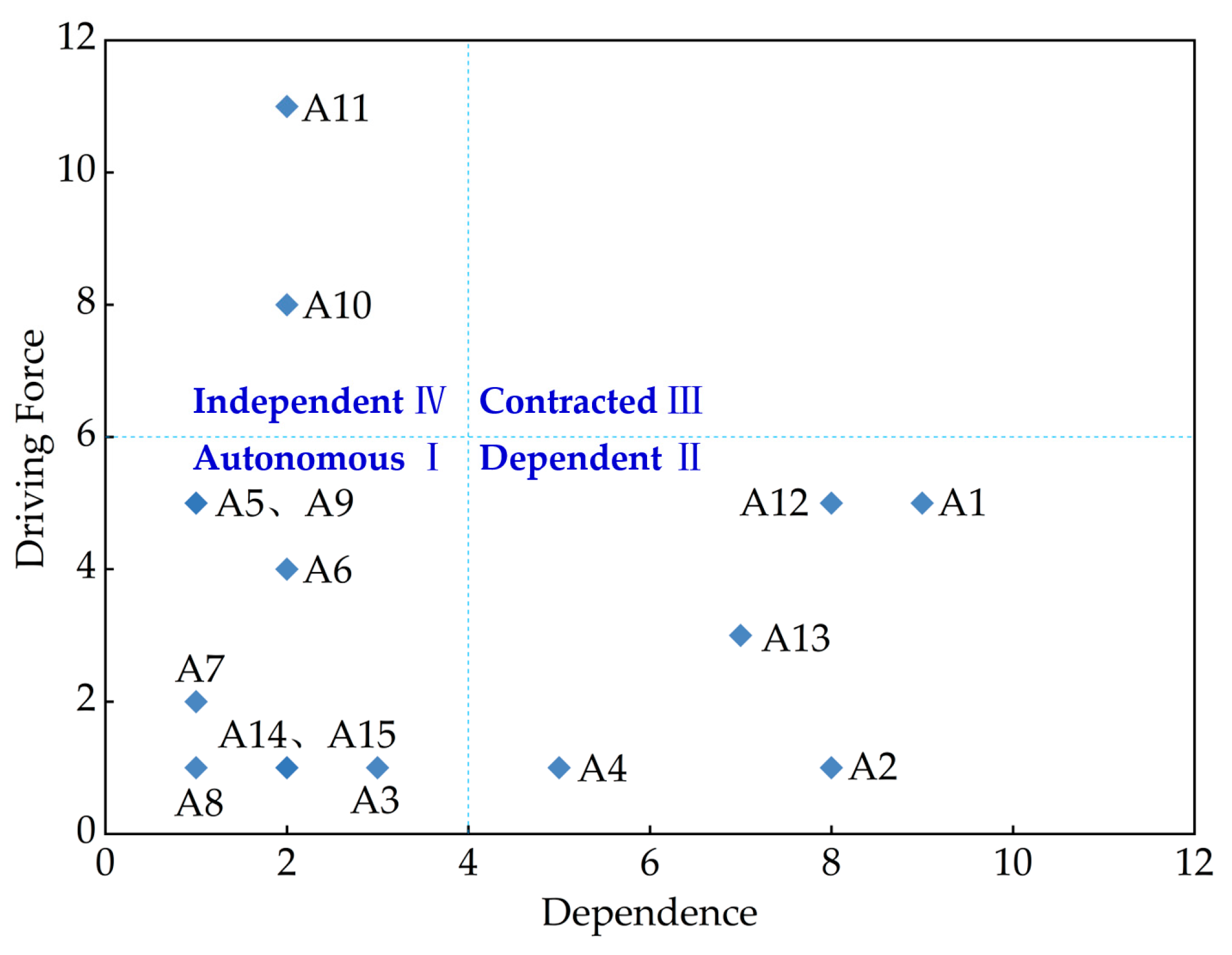
• Water resource abundance and scarcity (A10) and water availability (A11) are key factors with strong driving forces and low dependency that influence other factors. However, the dependent factors, namely socioeconomic development level (A1), regional industrial structure (A2), affordability to water users (A4), cost of the project’s water supply (A12), and guaranteed water supply rate (A13), are also key factors that require attention because of their strong influence on the results.
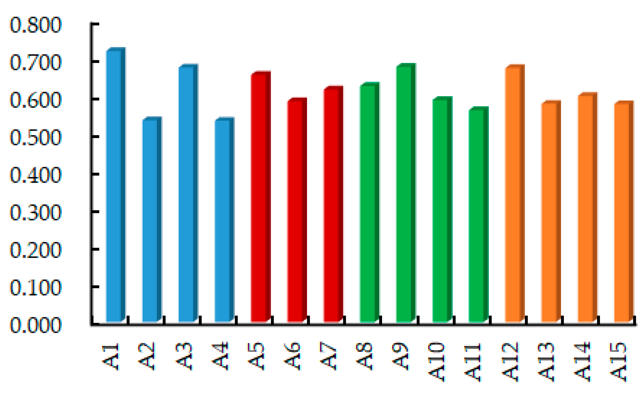
• Based on the GRA method, the top five factors influencing the water price for IWTPs were determined as follows: socioeconomic development level (A1), diversification of water resources (A9), water demand of water users (A3), cost of project’s water supply (A12), and national policies and regulations (A5).
• By investigating the factors influencing the water price for IWTPs, the effectiveness of the fuzzy DIM and GRA methods in studying the degree of influencing factors and the method of determining key factors were verified. Furthermore, determining the adjacency matrix of the ISM by setting a threshold is more objective than the previously used expert determination methods.

As this study mainly examined the interaction of factors affecting the formulation of water prices for IWTPs in China, the results can be applied to similar countries and regions. However, this study had certain limitations. Owing to the involvement of multiple aspects, stakeholders and links in the formulation of water prices for IWTPs, the influencing factors are complex. In future research, the methods and scope of the influencing factors can be further expanded, and model methods for identifying, screening, and determining factors can be optimized to comprehensively explore the factors influencing water price formulation from multiple perspectives, such as different links and stakeholders.

References

1. Tu, Y.; Wang, H.Y.; Zhou, X.Y.; Shen, W.J.; Lev, B. Comprehensive evaluation of security, equity, and efficiency on regional water resources coordination using a hybrid multi-criteria decision-making method with different hesitant fuzzy linguistic term sets. J. Clean. Prod. 2021, 310, 127447. [Google Scholar] [CrossRef]
2. Schlamovitz, J.L.; Becker, P. Differentiated vulnerabilities and capacities for adaptation to water shortage in Gaborone, Botswana. Int. J. Water Resour. Dev. 2021, 37, 278–299. [Google Scholar] [CrossRef]
3. Rehman, R.; Aslam, M.S.; Jasińska, E.; Javed, M.F.; Goňo, M. Guidelines for the Technical Sustainability Evaluation of the Urban Drinking Water Systems Based on Analytic Hierarchy Process. Resources 2023, 12, 8. [Google Scholar] [CrossRef]
4. Siddik, M.A.; Dickson, K.E.; Rising, J.; Ruddell, B.L.; Marston, L.T. Interbasin water transfers in the United States and Canada. Sci. Data 2023, 10, 27. [Google Scholar] [CrossRef] [PubMed]
5. Yan, B.W.; Chen, L. Coincidence probability of precipitation for the middle route of South-to-North water transfer project in China. J. Hydrol. 2013, 499, 19–26. [Google Scholar] [CrossRef]
6. Pasi, N.; Smardon, R. Inter-mmlinking of rivers: A solution for water crisis in india or a decision in doubt. J. Sci. Policy Gov. 2012, 2, 1. [Google Scholar]
7. Liu, J.G.; Zang, C.F.; Tian, S.Y.; Liu, J.G.; Yang, H.; Jia, S.F.; You, L.Z.; Liu, B.; Zhang, M. Water conservancy projects in China: Achievements, challenges and way forward. Glob. Environ. Change-Hum. Policy Dimens. 2013, 23, 633–643. [Google Scholar] [CrossRef]
8. Su, Q.M.; Chen, X. Efficiency analysis of metacoupling of water transfer based on the parallel data envelopment analysis model: A case of the South-North Water Transfer Project-Middle Route in China. J. Clean. Prod. 2021, 313, 127952. [Google Scholar] [CrossRef]
9. Sun, S.; Tang, Q.H.; Konar, M.; Fang, C.L.; Liu, H.X.; Liu, X.C.; Fu, G.T. Water transfer infrastructure buffers water scarcity risks to supply chains. Water Res. 2023, 229, 119442. [Google Scholar] [CrossRef]
10. Bui, D.T.; Talebpour Asl, D.; Ghanavati, E.; Al-Ansari, N.; Khezri, S.; Chapi, K.; Amini, A.; Pham, B.T. Effects of Inter-Basin Water Transfer on Water Flow Condition of Destination Basin. Sustainability 2020, 12, 338. [Google Scholar] [CrossRef]
11. Rogers, S.; Chen, D.; Jiang, H.; Rutherfurd, I.; Wang, M.; Webber, M.; Crow-Miller, B.; Barnett, J.; Finlayson, B.; Jiang, M.; et al. An integrated assessment of China’s South–North Water Transfer Project. Geogr. Res. 2019, 58, 49–63. [Google Scholar] [CrossRef]
12. Naghani, S.S.; Moghaddam, M.A.; Monfared, S.A.H. Inter-basin water transfer: A sustainable solution or an ephemeral painkiller to water shortage? Environ. Dev. Sustain. 2024, 26, 23025–23058. [Google Scholar] [CrossRef]
13. Wang, X.D.; Hu, C.M.; Liang, J.; Wang, J.; Dong, S.Y. A Study of the factors influencing the construction risk of steel truss bridges based on the improved DEMATEL-ISM. Buildings 2023, 13, 41. [Google Scholar] [CrossRef]
14. Liu, W.; Huang, Q.C. Research on Carbon Footprint Accounting in the Materialization Stage of Prefabricated Housing Based on DEMATEL-ISM-MICMAC. Appl. Sci. 2023, 13, 13148. [Google Scholar] [CrossRef]
15. He, L. Study on risk factors of substation construction project based on DEMATEL. Proj. Manag. Technol. 2024, 22, 18–21. [Google Scholar]
16. Chen, Z.; Huang, P.; Huang, W. Group intelligence fusion emergency decision-making method with dual-driven DEMATEL in a social network environment. J. Saf. Environ. 2024, 24, 2336–2347. [Google Scholar]
17. Zhang, J.; Li, J.; You, J.W. Research on Influencing Factors of Cost Control of Centralized Photovoltaic Power Generation Project Based on DEMATEL-ISM. Sustainability 2024, 16, 5289. [Google Scholar] [CrossRef]
18. Liu, W.; Hu, Y.H.; Huang, Q.C. Research on Critical Factors Influencing Organizational Resilience of Major Transportation Infrastructure Projects: A Hybrid Fuzzy DEMATEL-ISM-MICMAC Approach. Buildings 2024, 14, 1598. [Google Scholar] [CrossRef]
19. Xie, J.H.; Tian, F.J.; Li, X.Y.; Chen, Y.Q.; Li, S.Y. A study on the influencing factors and related paths of farmer’s participation in food safety governance-based on DEMATEL-ISM-MICMAC model. Sci. Rep. 2023, 13, 11372. [Google Scholar] [CrossRef]
20. Li, H.B.; Xiang, Y.R.; Xia, Y.H.; Yang, W.J.; Tang, X.T.; Lin, T. What Are the Obstacles to Promoting Photovoltaic Green Roofs in Existing Buildings? The Integrated Fuzzy DEMATEL-ISM-ANP Method. Sustainability 2023, 15, 16862. [Google Scholar] [CrossRef]
21. Liu, T.; Wang, P.; Cao, J.; He, Y.; Weng, Z. Internet-based recycling by urban residents in China: Evaluation of influencing factors using DEMATEL and ISM. Int. J. Environ. Sci. Technol. 2025, 22, 2517–2530. [Google Scholar] [CrossRef]
22. Luo, X.; Huang, X. Research on Cost Control of Prefabricated Building Based on Interpretative Structural Modeling Method. Constr. Econ. 2021, 42, 73–77. [Google Scholar]
23. Li, L.; Bai, F.; Mao, B.; Lei, Y. Research on the High-quality Developmentof Green Building Based on ISM-MICMAC: A Case Study of Shenyang. Constr. Econ. 2022, 43, 98–104. [Google Scholar]
24. Zheng, Y.; Shi, H. Research on Hierarchical Relationship of Influencing Factors of Green Building Development Based on ISM. J. Anhui Inst. Archit. Ind. 2022, 30, 83–89. [Google Scholar]
25. Tan, T.; Chen, K.; Xue, F.; Lu, W.S. Barriers to Building Information Modeling (BIM) implementation in China’s prefabricated construction: An interpretive structural modeling (ISM) approach. J. Clean. Prod. 2019, 219, 949–959. [Google Scholar] [CrossRef]
26. Deng, J.X.; Li, X.X.; Rao, J.T. Research on Influencing Factors and Driving Path of BIM Application in Construction Projects Based on the SD Model in China. Buildings 2023, 13, 2794. [Google Scholar] [CrossRef]
27. Yuan, H.P.; Yang, Y. BIM Adoption under Government Subsidy: Technology Diffusion Perspective. J. Constr. Eng. Manag. 2020, 146, 04019089. [Google Scholar] [CrossRef]
28. Xu, H.Y.; Chang, R.D.; Dong, N.; Zuo, J.; Webber, R.J. Interaction mechanism of BIM application barriers in prefabricated construction and driving strategies from stakeholders’ perspectives. Ain Shams Eng. J. 2023, 14, 101821. [Google Scholar] [CrossRef]
29. Jang, S.; Lee, G. Process, productivity, and economic analyses of BIM based multi-trade prefabrication—A case study. Autom. Constr. 2018, 89, 86–98. [Google Scholar] [CrossRef]
30. Lin, M.C.; Ren, Y.F.; Feng, C.; Li, X.J. Analyzing resilience influencing factors in the prefabricated building supply chain based on SEM-SD methodology. Sci. Rep. 2024, 14, 17393. [Google Scholar] [CrossRef]
31. Belay, S.; Goedert, J.; Woldesenbet, A.; Rokooei, S.; Matos, J.; Sousa, H. Key BIM Adoption Drivers to Improve Performance of Infrastructure Projects in the Ethiopian Construction Sector: A Structural Equation Modeling Approach. Adv. Civ. Eng. 2021, 2021, 7473176. [Google Scholar] [CrossRef]
32. Chang, C.Y.; Pan, W.J.; Howard, R. Impact of Building Information Modeling Implementation on the Acceptance of Integrated Delivery Systems: Structural Equation Modeling Analysis. J. Constr. Eng. Manag. 2017, 143, 04017044. [Google Scholar] [CrossRef]
33. Wang, P.; Yu, Y. Research on Influencing Factors of Resilience of High-tech Ship Industry Chain Based on Fuzzy DEMATEL-ISM. Sci. Technol. Manag. Res. 2023, 43, 196–204. [Google Scholar]
34. Zhu, W.X.; Zhang, J.; Wang, D.; Ma, C.S.; Zhang, J.F.; Chen, P. Study on the Critical Factors Influencing High-Quality Development of Green Buildings for Carbon Peaking and Carbon Neutrality Goals of China. Sustainability 2023, 15, 5035. [Google Scholar] [CrossRef]
35. Mustafa, M.; Malik, M.O.F. Factors Hindering Solar Photovoltaic System Implementation in Buildings and Infrastructure Projects: Analysis through a Multiple Linear Regression Model and Rule-Based Decision Support System. Buildings 2023, 13, 1786. [Google Scholar] [CrossRef]
36. Hu, W.; Kong, D.; He, X. Analysis on Influencing Factors of Green Building Development Based on BP-WINGS. Soft Sci. 2020, 34, 75–81. [Google Scholar]
37. Peng, Z.Y.; Yin, J.X.; Zhang, L.L.; Zhao, J.; Liang, Y.; Wang, H. Assessment of the Socio-Economic Impact of a Water Diversion Project for a Water-Receiving Area. Pol. J. Environ. Stud. 2020, 29, 1771–1784. [Google Scholar] [CrossRef]
38. Schnuelle, C.; Wassermann, T.; Stuehrmann, T. Mind the Gap-A Socio-Economic Analysis on Price Developments of Green Hydrogen, Synthetic Fuels, and Conventional Energy Carriers in Germany. Energies 2022, 15, 3541. [Google Scholar] [CrossRef]
39. Chen, M.; Wang, K. The combining and cooperative effects of carbon price and technological innovation on carbon emission reduction: Evidence from China’s industrial enterprises. J. Environ. Manag. 2023, 343, 118188. [Google Scholar] [CrossRef]
40. Vidal-Lamolla, P.; Molinos-Senante, M.; Poch, M. Understanding the Residential Water Demand Response to Price Changes: Measuring Price Elasticity with Social Simulations. Water 2024, 16, 2501. [Google Scholar] [CrossRef]
41. Marlim, M.S.; Kang, D.S. Improving operational efficiency in water distribution network with hourly water pricing to benefit consumers and providers. J. Water Process Eng. 2025, 72, 107457. [Google Scholar] [CrossRef]
42. Marques, G.; Possantti, I.; Dalcin, A.P.; Daiello, J.; Gonzalez, I.; Todeschini, F.; Goldenfum, J. An integrated hydro-finance approach towards sustainable urban stormwater and flood control management. J. Clean. Prod. 2024, 470, 143364. [Google Scholar] [CrossRef]
43. Jia, J.J.; Liang, Q.; Jiang, M.R.; Wu, H.Q. Household water price and income elasticities under increasing-block pricing policy in China: An estimation using nationwide large-scale survey data. Environ. Res. Commun. 2024, 6, 061002. [Google Scholar] [CrossRef]
44. Zhang, G.J.; Wu, H.Q.; Liu, Y.Z.; Chen, X.; Song, P.F. Does Residents’ Perception of Information Influence the Implementation Effect of Increasing-Block Water Pricing Policy? Water Econ. Policy 2024, 10. [Google Scholar] [CrossRef]
45. Gao, Y.; Chen, C.; Wu, L.; Liu, J.; Li, D.; Wang, G. Demand analysis of urban reclaimed water considering water quality and water price. J. Water Resour. Water Eng. 2024, 35, 60–70. [Google Scholar]
46. Hughes, N.; Gupta, M.; Whittle, L.; Westwood, T. An Economic Model of Spatial and Temporal Water Trade in the Australian Southern Murray-Darling Basin. Water Resour. Res. 2023, 59, e2022WR032559. [Google Scholar] [CrossRef]
47. Ribeiro, F.W.; da Silva, S.M.O.; de Souza, F.D.; Carvalho, T.M.N.; Lopes, T. Diversification of urban water supply: An assessment of social costs and water production costs. Water Policy 2022, 24, 980–997. [Google Scholar] [CrossRef]
48. Yu, H.; Ge, J.J. Recent advances in Ru-based electrocatalysts toward acid electrochemical water oxidation. Curr. Opin. Electrochem. 2023, 39, 101296. [Google Scholar] [CrossRef]
49. Cooper, B.; Burton, M.; Crase, L. Exploring customer heterogeneity with a scale-extended latent class choice model: Experimental evidence drawn from urban water users. Aust. J. Agric. Resour. Econ. 2023, 67, 176–197. [Google Scholar] [CrossRef]
50. Liu, Y.; Chong, F.T.; Jia, J.J.; Cao, S.L.; Wang, J. Proper Pricing Approach to the Water Supply Cost Sharing: A Case Study of the Eastern Route of the South to North Water Diversion Project in China. Water 2022, 14, 2842. [Google Scholar] [CrossRef]
51. Qin, C.H.; Jiang, S.; Zhao, Y.; Zhu, Y.N.; Wang, Q.M.; Wang, L.Z.; Qu, J.L.; Wang, M. Research on Water Rights Trading and Pricing Model between Agriculture and Energy Development in Ningxia, China. Sustainability 2022, 14, 15748. [Google Scholar] [CrossRef]
52. Wang, S.W.; Liu, S.B.; Yao, S.P.; Guo, X.; Soomro, S.E.H.; Niu, C.J.; Quan, L.Y.; Hu, C.H. Game Theory Applications in Equilibrium Water Pricing of Multiple Regional Sources and Users. Water 2024, 16, 1845. [Google Scholar] [CrossRef]
53. Hur, A.Y.; Page, M.A.; Guest, J.S.; Ploschke, C.M. Financial analysis of decentralized water reuse systems in mission critical facilities at US Army installations. Environ. Sci. Water Res. Technol. 2024, 10, 603–613. [Google Scholar] [CrossRef]
54. Nawar, B.; Scardigno, A.; Sagardoy, J.A. Treatment and reuse of water: Economic feasibility and assessment of water pricing policies in Ouardanine irrigation district (Tunisia). NEW MEDIT 2024, 23, 73–93. [Google Scholar] [CrossRef]
55. Berbel, J.; Gutierrez-Marín, C.; Expósito, A. Impacts of irrigation efficiency improvement on water use, water consumption and response to water price at field level. Agric. Water Manag. 2018, 203, 423–429. [Google Scholar] [CrossRef]
56. Ma, L.; Wang, Q. Do Water Transfer Projects Promote Water Use Efficiency? Case Study of South-to-North Water Transfer Project in Yellow River Basin of China. Water 2024, 16, 1367. [Google Scholar] [CrossRef]
57. Peng, X.; Li, N.N. Water Pricing Mechanism for China’s South-to-North Water Diversion Project: Design, Evaluation, and Suggestions. J. Am. Water Resour. Assoc. 2022, 58, 1230–1239. [Google Scholar] [CrossRef]
58. Chen, L.; Xiao, H.; Liu, X.; Liu, W. Sensitivity analysis of influencing factors of open-pit mine slope stability based on grey correlation. Bull. Surv. Mapp. 2024, 1, 145–149. [Google Scholar] [CrossRef]
59. Marlin, D.; Lamont, B.T.; Hoffman, J.J. Choice situation, strategy, and performance: A reexamination. Strateg. Manag. J. 1994, 15, 229–239. [Google Scholar] [CrossRef]
60. Gunasekaran, J.; Sevvel, P.; John Solomon, I.; Vasanthe Roy, J. Multi objective optimization of parameters during FSW of AZ80A-AZ31B Mg alloys using grey relational analysis. J. Mech. Sci. Technol. 2024, 38, 4971–4982. [Google Scholar] [CrossRef]
61. Zhu, R.; Bhutta, Z.M.; Zhu, Y.; Ubaidullah, F.; Saleem, M.; Khalid, S. Grey relational analysis of country-level entrepreneurial environment: A study of selected forty-eight countries. Front. Environ. Sci. 2022, 10, 985426. [Google Scholar] [CrossRef]
62. Luo, M.; Wang, D.; Wang, X.; Lu, Z. Analysis of Surface Settlement Induced by Shield Tunnelling: Grey Relational Analysis and Numerical Simulation Study on Critical Construction Parameters. Sustainability 2023, 15, 14315. [Google Scholar] [CrossRef]
Figure 1. Research flowchart.
Water 17 02022 g001
Figure 2. Impact degree–affected degree diagram.
Water 17 02022 g002
Figure 3. Centrality–causal degree diagram.
Water 17 02022 g003
Figure 4. System graph of influencing factors.
Water 17 02022 g004
Figure 5. Multilevel ISM.
Water 17 02022 g005
Figure 6. MICMAC classification chart of influencing factors.
Water 17 02022 g006
Figure 7. Correlation coefficients.
Water 17 02022 g007
Figure 8. Correlation degrees.
Water 17 02022 g008