
Improved Groundwater Arsenic Contamination Modeling Using 3-D Stratigraphic Mapping, Eastern Wisconsin, USA

Abstract
1. Introduction
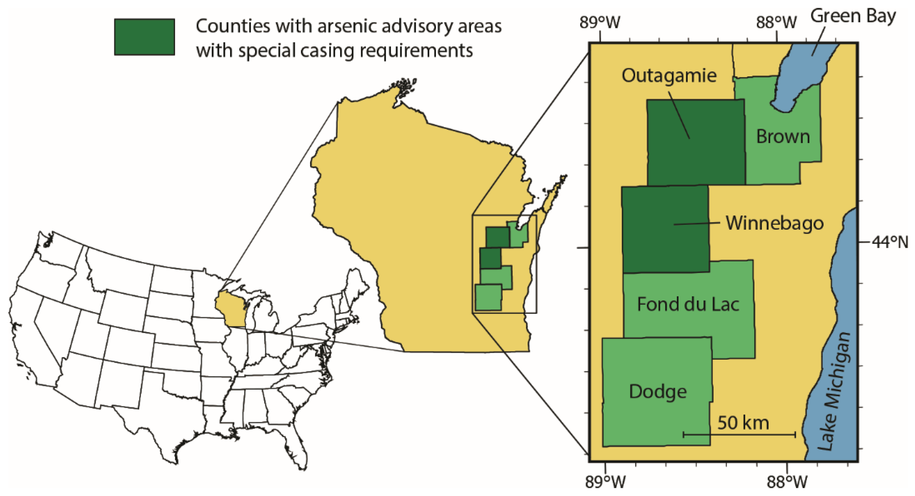
2. Regional Setting
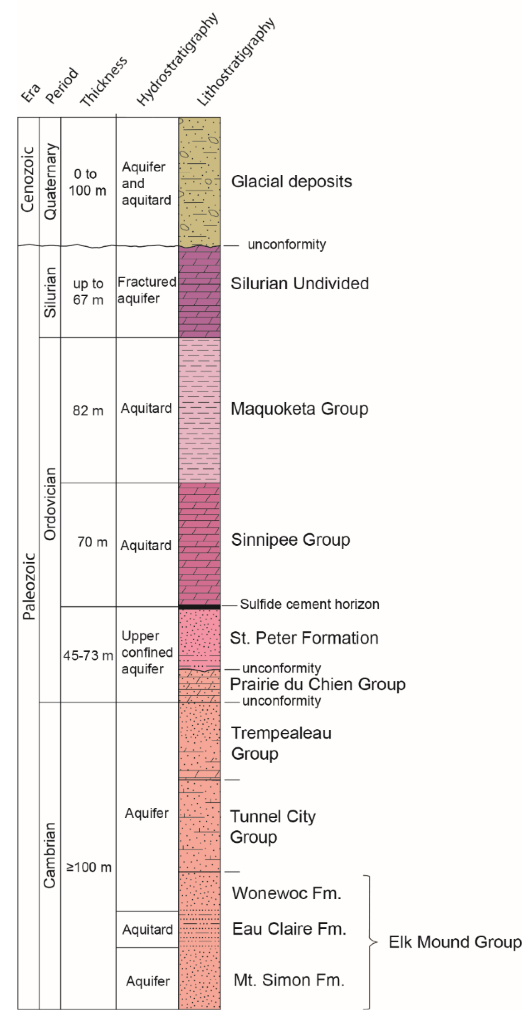
2.1. Geologic and Hydrogeologic Setting
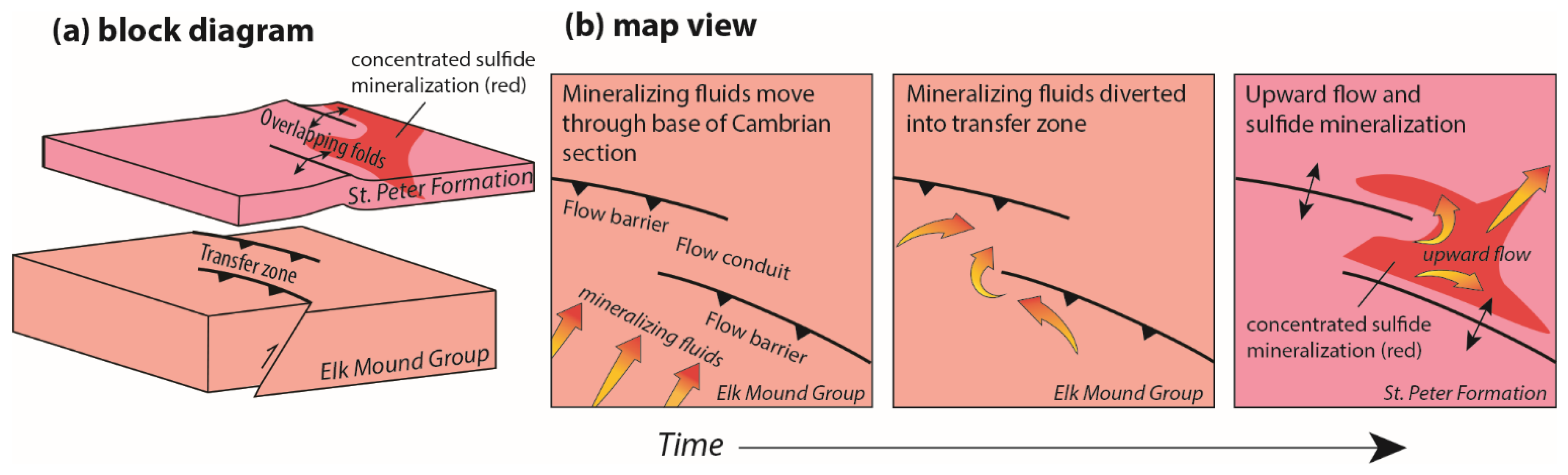
2.2. Arsenic Release Mechanisms and Geologic Sources of Arsenic in Eastern Wisconsin
3. Materials and Methods
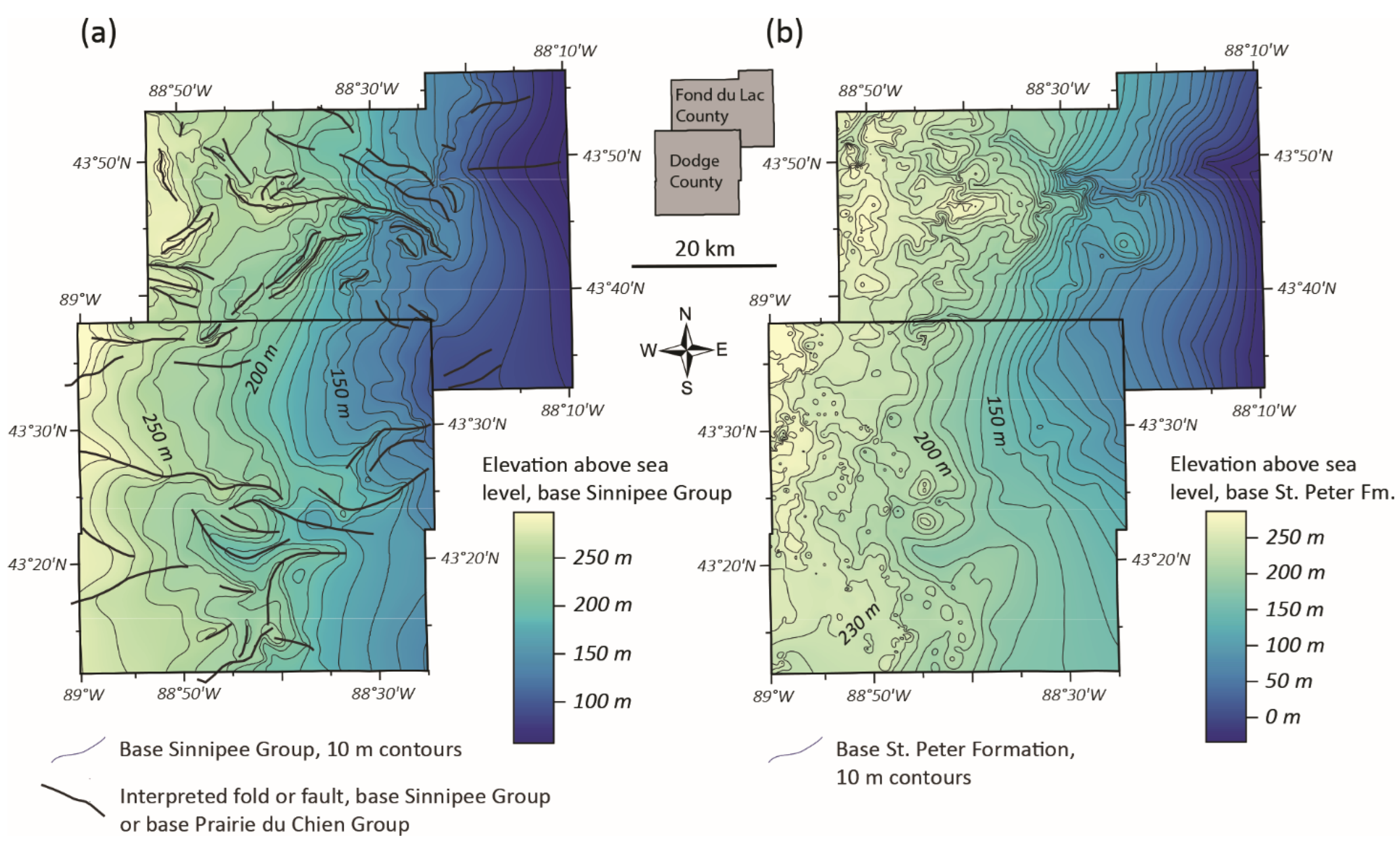
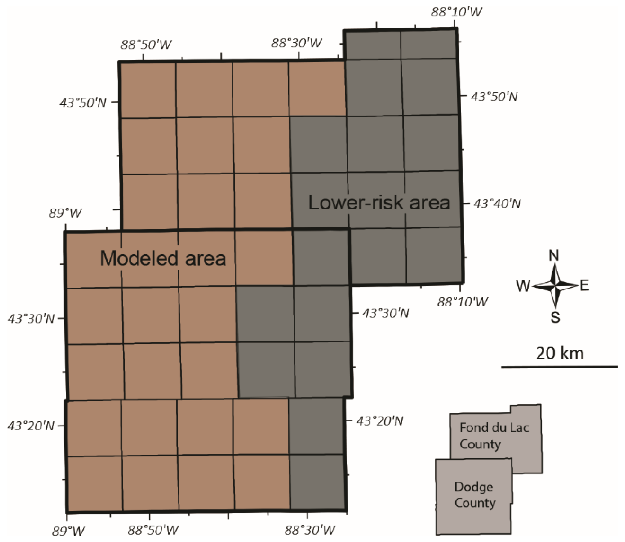
3.1. Construction of 3-D Geologic Surfaces
3.2. Well Data
3.3. Binary Logistic Regression
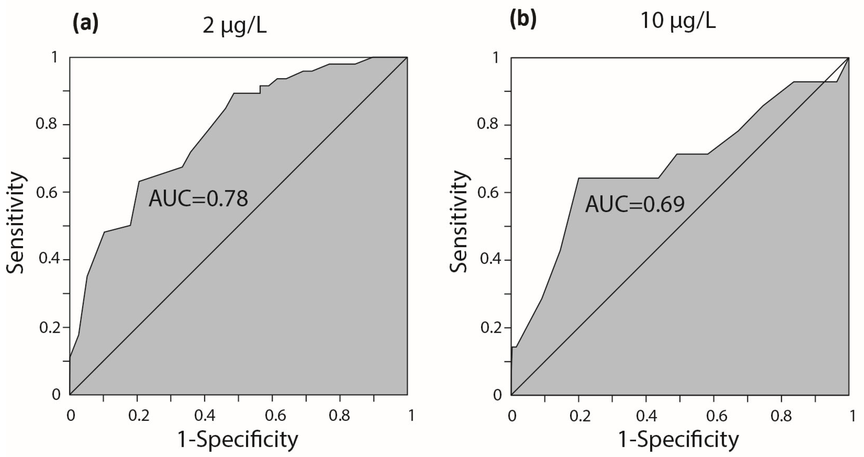
3.4. Model Fit and Assessment
4. Results
4.1. Three-Dimensional Geologic Surfaces
4.2. Well Data
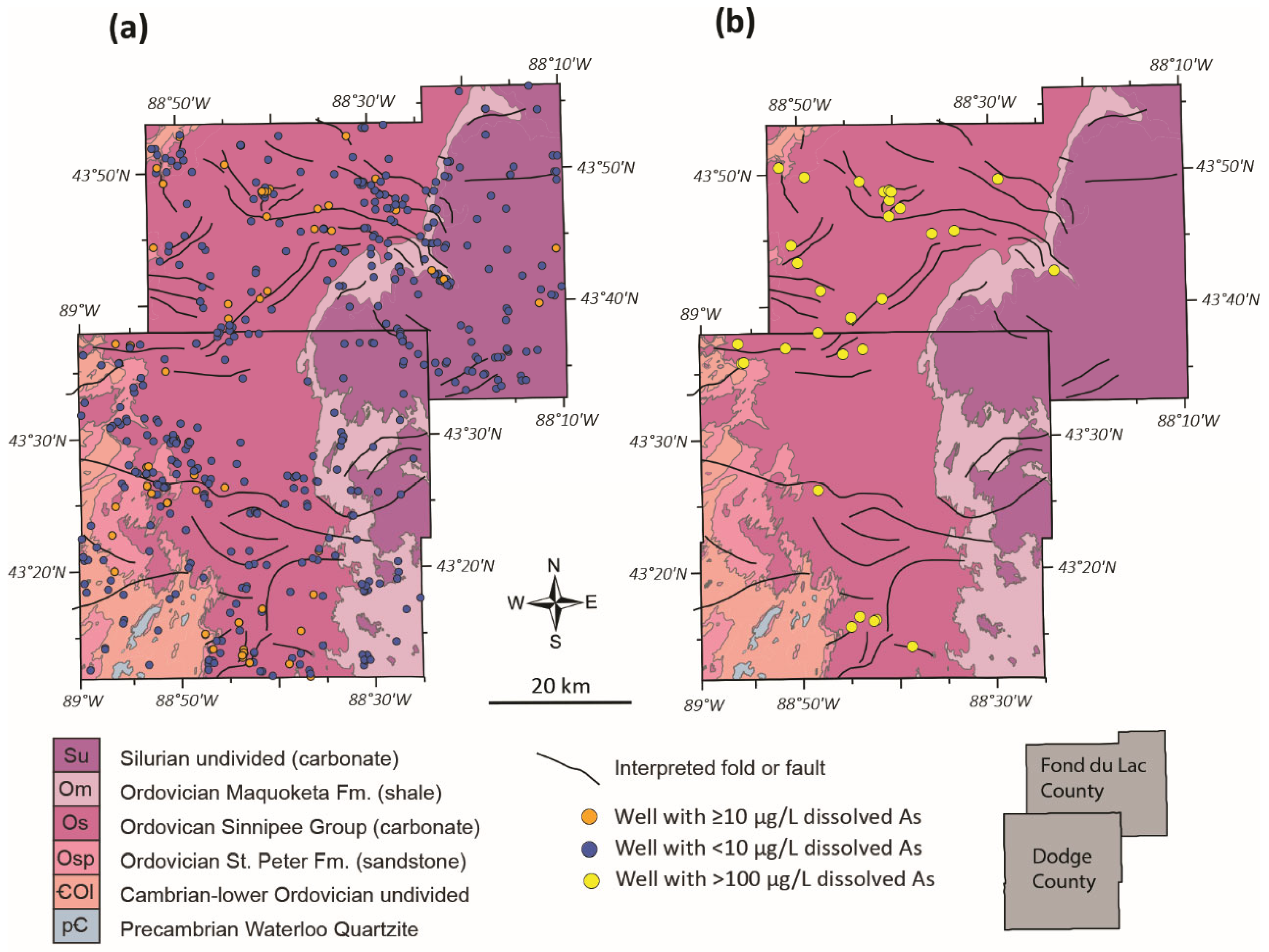
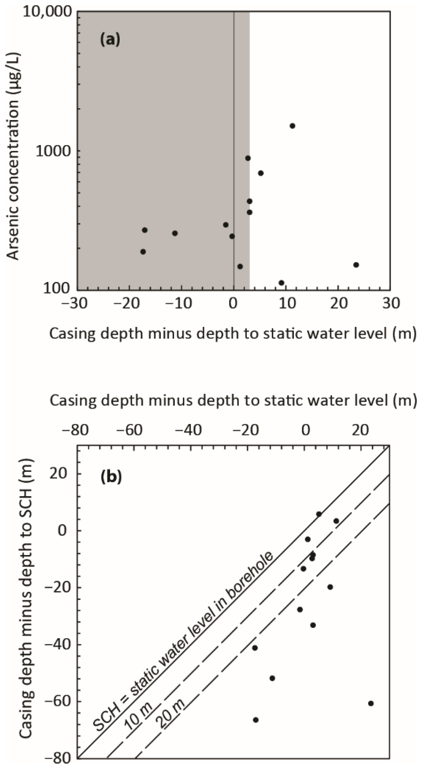
4.2.1. High Arsenic Values (>100 µg/L)
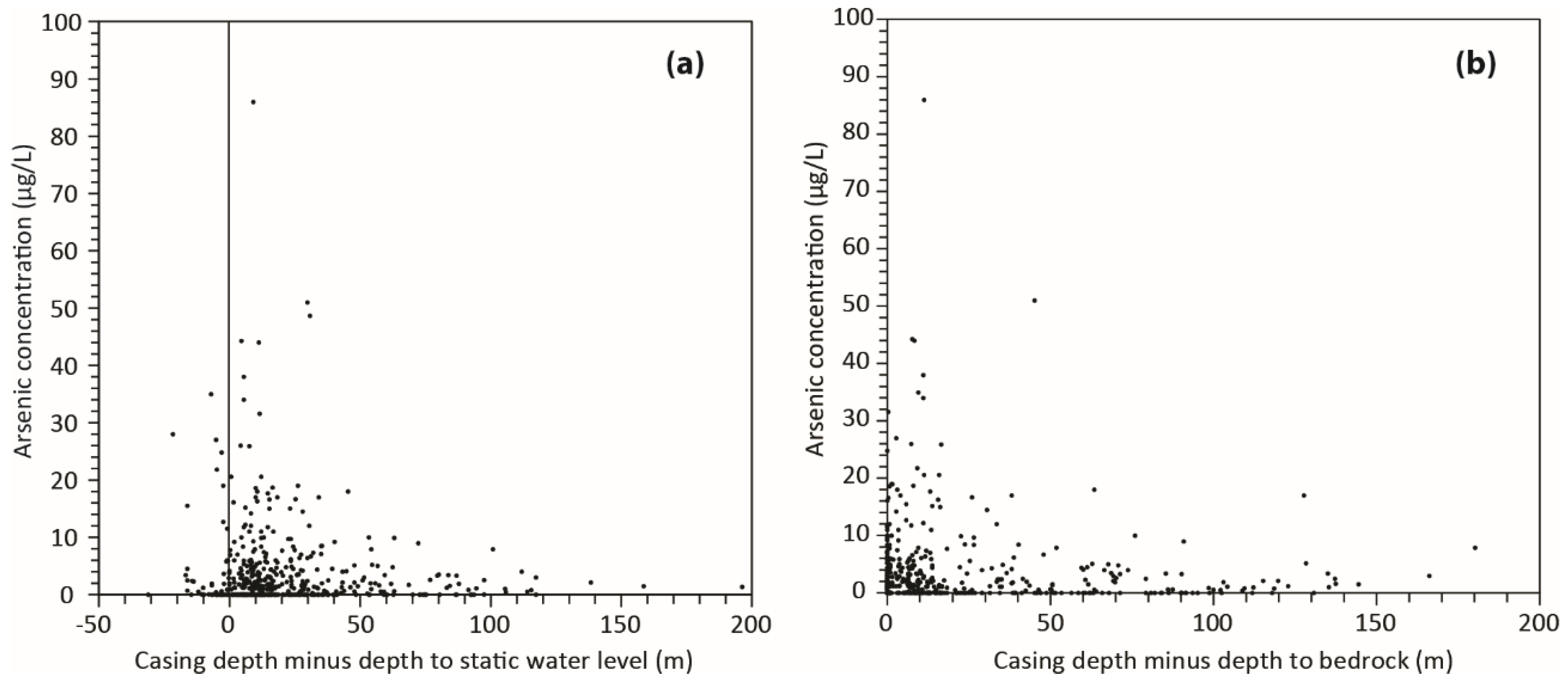
4.2.2. Low to Moderate Arsenic Values (0 to 100 µg/L)
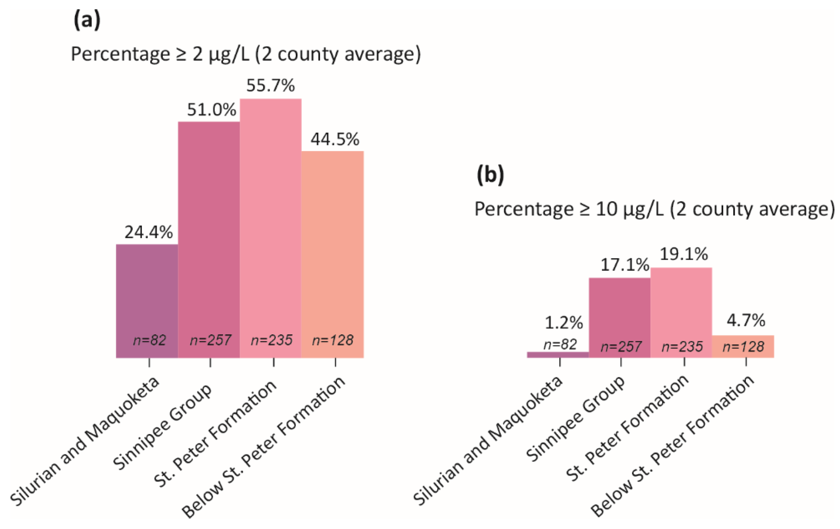
4.2.3. Role of Geologic Units in Arsenic Detection
4.3. Logistic Regression Results
5. Discussion
5.1. Causes of Arsenic in Groundwater in Fond Du Lac and Dodge Counties
5.2. Applications
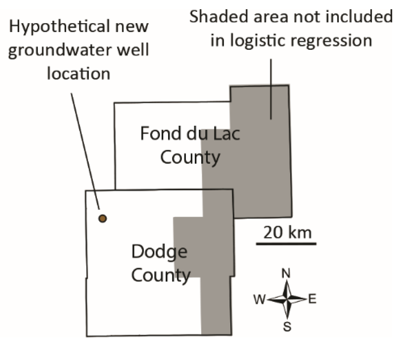
5.2.1. Construction of new groundwater wells
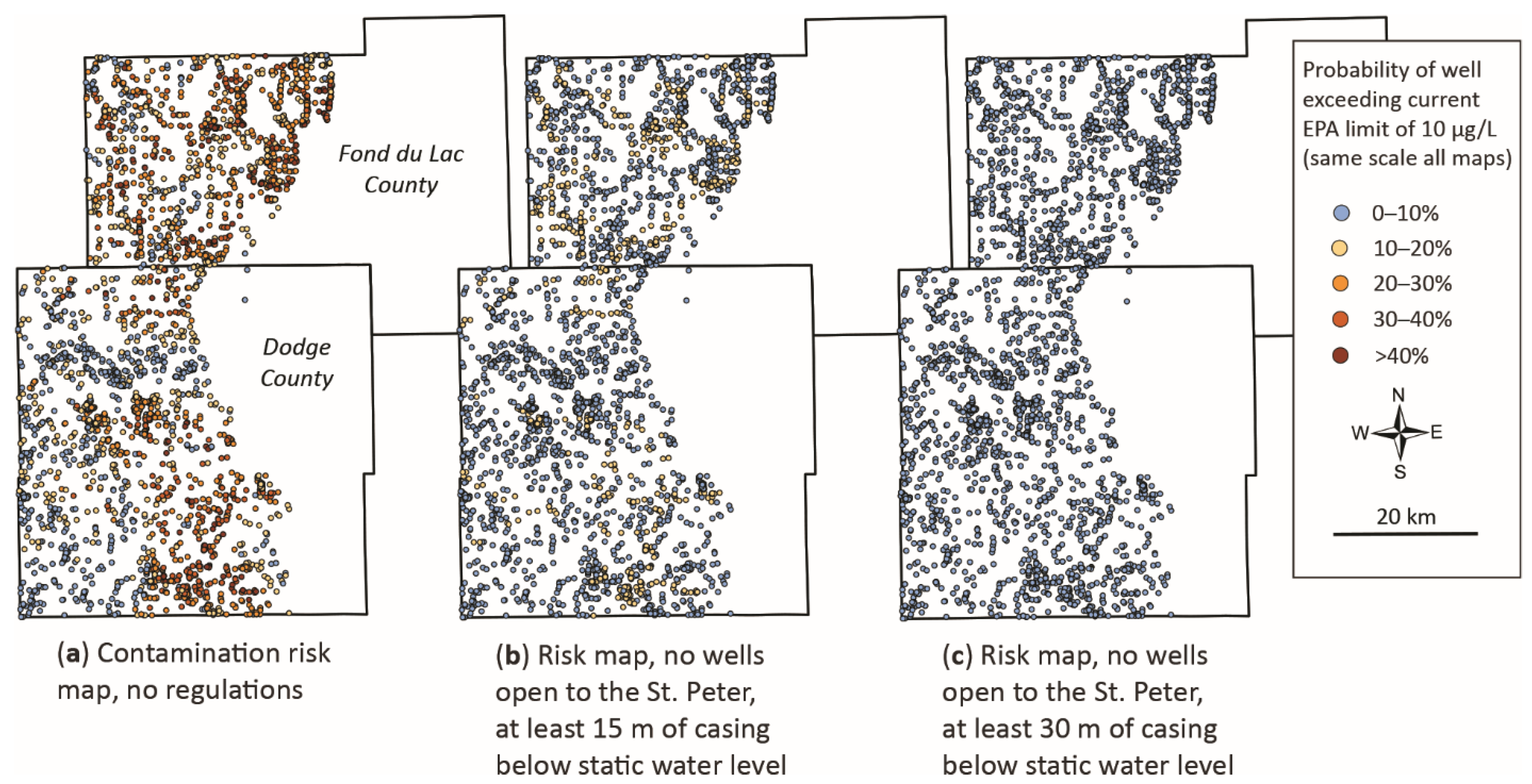
5.2.2. Evaluation of Risk to Existing Groundwater Wells, and Impact of Casing Requirements
6. Conclusions and Future Work
Supplementary Materials
Author Contributions
Funding
Data Availability Statement
Acknowledgments
Conflicts of Interest
Abbreviations
| SCH | Sulfide cement horizon |
| WDNR | Wisconsin Department of Natural Resources |
| EPA MCL | Environmental Protection Agency Maximum Contaminant Level |
References
- Ayotte, J.D.; Nolan, B.T.; Nuckols, J.R.; Cantor, K.P.; Robinson, G.R.; Baris, D.; Hayes, L.; Karagas, M.; Bress, W.; Silverman, D.T.; et al. Modeling the probability of arsenic in groundwater in New England as a tool for exposure assessment. Environ. Sci. Technol. 2006, 40, 3578–3585. [Google Scholar] [CrossRef]
- Kim, D.; Miranda, M.L.; Tootoo, J.; Bradley, P.; Gelfand, A.E. Spatial modeling for groundwater arsenic levels in North Carolina. Environ. Sci. Technol. 2011, 45, 4824–4831. [Google Scholar] [CrossRef]
- VanDerwerker, T.; Zhang, L.; Ling, E.; Benham, B.; Schreiber, M. Evaluating geologic sources of arsenic in well water in Virginia (USA). Int. J. Environ. Res. Public Health 2018, 15, 787. [Google Scholar] [CrossRef]
- Berg, R.C.; Russell, H.A.J.; Thorleifson, L.H. Introduction to a Special Issue on Three-dimensional Geological Mapping for Groundwater Applications. J. Maps 2007, 3, 211–218. [Google Scholar] [CrossRef]
- Pavlis, T.L.; Mason, K.A. The new world of 3D geologic mapping. GSA Today 2017, 27, 4–10. [Google Scholar] [CrossRef]
- Burkel, R.S.; Stoll, R.C. Naturally occurring arsenic in sandstone aquifer water supply wells of northeastern Wisconsin. Groundw. Monit. Remediat. 1999, 19, 114–121. [Google Scholar] [CrossRef]
- Root, T.L.; Gotkowitz, M.B.; Bahr, J.M.; Attig, J.W. Arsenic geochemistry and hydrostratigraphy in Midwestern US glacial deposits. Groundwater 2010, 48, 903–912. [Google Scholar] [CrossRef] [PubMed]
- Erickson, M.L.; Barnes, R.J. Glacial sediment causing regional-scale elevated arsenic in drinking water. Groundwater 2005, 43, 796–805. [Google Scholar] [CrossRef]
- Erickson, M.L.; Elliott, S.M.; Brown, C.J.; Stackelberg, P.E.; Ransom, K.M.; Reddy, J.E.; Cravotta, C.A., III. Machine-learning predictions of high arsenic and high manganese at drinking water depths of the glacial aquifer system, northern continental United States. Environ. Sci. Technol. 2021, 55, 5791–5805. [Google Scholar] [CrossRef]
- Stewart, E.K. Bedrock Geology of Dodge County; Map 508, 7, 1 pl., scale 1:100,000; Wisconsin Geological and Natural History Survey: Madison, WI, USA, 2021; Available online: https://wgnhs.wisc.edu/pubs/000975 (accessed on 20 June 2025).
- Muldoon, M.A.; Simo, J.A.; Bradbury, K.R. Correlation of hydraulic conductivity with stratigraphy in a fractured-dolomite aquifer, northeastern Wisconsin, USA. Hydrogeol. J. 2001, 9, 570–583. [Google Scholar] [CrossRef]
- Hart, D.J.; Bradbury, K.R.; Feinstein, D.T. The vertical hydraulic conductivity of an aquitard at two spatial scales. Groundwater 2006, 44, 201–211. [Google Scholar] [CrossRef] [PubMed]
- Eaton, T.T.; Anderson, M.P.; Bradbury, K.R. Fracture control of ground water flow and water chemistry in a rock aquitard. Groundwater 2007, 45, 601–615. [Google Scholar] [CrossRef] [PubMed]
- Schreiber, M.E.; Simo, J.A.; Freiberg, P.G. Stratigraphic and geochemical controls on naturally occurring arsenic in groundwater, eastern Wisconsin, USA. Hydrogeol. J. 2000, 8, 161–176. [Google Scholar] [CrossRef]
- Schreiber, M.E.; Gotkowitz, M.B.; Simo, J.A.; Freiberg, P.G. Mechanisms of arsenic release to ground water from naturally occurring sources, eastern Wisconsin. In Arsenic in Ground Water: Geochemistry and Occurrence; Welch, A.H., Stollenwerk, K.G., Eds.; Springer: Boston, MA, USA, 2003; pp. 259–280. [Google Scholar] [CrossRef]
- Gotkowitz, M.B.; Schreiber, M.E.; Simo, J.A. Effects of water use on arsenic release to well water in a confined aquifer. Groundwater 2004, 42, 568–575. [Google Scholar] [CrossRef]
- Luczaj, J.A.; McIntire, M.J.; Hunt, J.O. Geochemical characterization of trace MVT mineralization in Paleozoic sedimentary rocks of northeastern Wisconsin, USA. Geosciences 2016, 6, 29. [Google Scholar] [CrossRef]
- Stewart, E.D.; Stewart, E.K.; Bradbury, K.R.; Fitzpatrick, W. Correlating bedrock folds to higher rates of arsenic detection in groundwater, southeast Wisconsin, USA. Groundwater 2021, 59, 829–838. [Google Scholar] [CrossRef]
- Fitzpatrick, W.A.; Stewart, E.D. Geologic map of the Highland East and West 7.5-minute Quadrangles, Grant and Iowa Counties, Wisconsin; Map 510, 15, 1 pl., scale 1:24,000; Wisconsin Geological and Natural History Survey: Madison, WI, USA, 2024. [Google Scholar] [CrossRef]
- Stewart, E.D.; Mauel, S.W.; Batten, W.G. Geologic Map of the Stitzer and Western Part of the Montfort 7.5-minute Quadrangles; Open-File Report 2023–03, 1 pl., scale 1:24,000; Wisconsin Geological and Natural History Survey: Madison, WI, USA, 2023. [Google Scholar] [CrossRef]
- Stewart, E.D.; Mauel, S.W.; Bremmer, S.E.; Fitzpatrick, W.A. Bedrock geology of Grant County, Wisconsin; Bulletin 119, 33 p., 1 pl., scale 1:100,000; Wisconsin Geological and Natural History Survey: Madison, WI, USA, 2025. [Google Scholar] [CrossRef]
- Hadley, D.R.; Abrams, D.B.; Roadcap, G.S. Modeling a large-scale historic aquifer test—Insight into the hydrogeology of a regional fault zone. Groundwater 2020, 58, 453–463. [Google Scholar] [CrossRef] [PubMed]
- Batten, W.G. Bedrock geology of Fond du Lac County; Map 505, 2 pl., scale 1:100,000; Wisconsin Geological and Natural History Survey: Madison, WI, USA, 2018; Available online: https://wgnhs.wisc.edu/catalog/publication/000963 (accessed on 20 June 2025).
- Stewart, E.K. Depth-to-Bedrock Map of Dodge County; Open-File Report 2021–03, 13 p., 1 pl., scale 1:100,000; Wisconsin Geological and Natural History Survey: Madison, WI, USA, 2021; Available online: https://wgnhs.wisc.edu/catalog/publication/000981 (accessed on 20 June 2025).
- Wisconsin Department of Natural Resources. Search Sample Analytical Data. Available online: https://dnr.wisconsin.gov/topic/Groundwater/GRN.html (accessed on 20 May 2020).
- Wisconsin Department of Natural Resources. Pump Works Data. Available online: https://en.wikipedia.org/wiki/Wisconsin_Department_of_Natural_Resources?ysclid=mcpynpcv2y334118609 (accessed on 8 March 2021).
- Wisconsin Geological and Natural History Survey. Well Construction Report Database. Available online: https://home.wgnhs.wisc.edu/ (accessed on 3 May 2021).
- Yang, Q.; Jung, H.B.; Marvinney, R.G.; Culbertson, C.W.; Zheng, Y. Can arsenic occurrence rates in bedrock aquifers be predicted? Environ. Sci. Technol. 2012, 46, 2080–2087. [Google Scholar] [CrossRef]
- Andy, C.M.; Fahnestock, M.F.; Lombard, M.A.; Hayes, L.; Bryce, J.G.; Ayotte, J.D. Assessing models of arsenic occurrence in drinking water from bedrock aquifers in New Hampshire. J. Contemp. Water Res. Educ. 2017, 160, 25–41. [Google Scholar] [CrossRef]
- Cao, H.; Xie, X.; Wang, Y.; Pi, K.; Li, J.; Zhan, H.; Liu, P. Predicting the risk of groundwater arsenic contamination in drinking water wells. J. Hydrol. 2018, 560, 318–325. [Google Scholar] [CrossRef]
- Hosmer, D.W.; Lemeshow Sturdivant, R.X. Applied Logistic Regression; John Wiley & Sons: Hoboken, NJ, USA, 2013. [Google Scholar]
- Hosmer, D.W.; Lemeshow, S. Goodness of fit tests for the multiple logistic regression model. Commun. Stat.–Theory Methods 1980, 9, 1043–1069. [Google Scholar] [CrossRef]
- Mai, H.; Dott, R.H., Jr. A Subsurface Study of the St. Peter Sandstone in Southern and Eastern Wisconsin; Information Circular, v. 47, 26 p., 2 pls., scale 1:750,000; Wisconsin Geological and Natural History Survey: Madison, WI, USA, 1985; Available online: https://wgnhs.wisc.edu/pubs/000297 (accessed on 20 June 2025).
- Devaul, R.W.; Harr, C.A.; Schiller, J.J. Ground-Water Resources and Geology of Dodge County, Wisconsin; Information Circular 44, 34 p., 1 plate, scale 1:125,000; Wisconsin Geological and Natural History Survey: Madison, WI, USA, 1983; Available online: https://wgnhs.wisc.edu/pubs/000294 (accessed on 20 June 2025).
- Knierim, K.J.; Kingsbury, J.A.; Belitz, K.; Stackelberg, P.E.; Minsley, B.J.; Rigby, J.R. Mapped predictions of manganese and arsenic in an alluvial aquifer using boosted regression trees. Groundwater 2022, 60, 362–376. [Google Scholar] [CrossRef] [PubMed]

| Variable Tested | Variable Type |
|---|---|
| Distance to nearest fold axis | Continuous |
| Well open to the Sinnipee Group | Categorical |
| Well open to St. Peter Formation | Categorical |
| Well open to units below St. Peter | Categorical |
| Casing depth minus depth to bedrock | Continuous |
| Casing depth minus depth to static water level | Continuous |
| 2 µg/L Cutoff (n = 283) | 10 µg/L Cutoff (n = 228) | ||||
|---|---|---|---|---|---|
| Variable | Variable Type | Variable (bi) Coefficient (Multivariate) | Odds Ratio | Variable (bi) Coefficient (Multivariate) | Odds Ratio |
| Intercept | N/A | 0.8398 (0.3556, 1.4274) | N/A | −0.3126 (−0.8671, 0.3436) | N/A |
| Distance to nearest fold axis 2 | Continuous | −0.3454 (−0.5215, −0.2254) | 0.7079 (0.5936, 0.7982) | −0.2689 (−0.5821, −0.0900) | 0.7642 (0.5587, 0.9139) |
| Well open to St. Peter Formation | Categorical | 0.6532 (0.1197, 1.2225) | 1.9216 (1.1271, 3.3956) | N/A | N/A |
| Well open to units below St. Peter | Categorical | N/A | N/A | −1.0684 (−2.9185, −0.1396) | 0.3436 (0.0540, 0.8697) |
| Casing depth minus depth to bedrock 3 | Continuous | −0.0184 (−0.0302, −0.0085) | 0.9818 (0.9703, 0.9915) | N/A | N/A |
| Casing depth minus depth to static water level 3 | Continuous | N/A | N/A | −0.0409 (−0.0804, −0.0026) | 0.9599 (0.9227, 0.9974) |
| 2 µg/L 2 | Actual Positive | Actual Negative | 10 µg/L 3 | Actual Positive | Actual Negative |
|---|---|---|---|---|---|
| Predicted Positive | 31 | 13 | Predicted Positive | 9 | 18 |
| Predicted negative | 15 | 26 | Predicted negative | 5 | 37 |
| 15 m Casing, 40 m Deep Well | 45 m Casing, 80 m Deep Well | |||
|---|---|---|---|---|
| 2 µg/L Cutoff | 10 µg/L Cutoff | 2 µg/L Cutoff | 10 µg/L Cutoff | |
| Probability of arsenic exceedance | 46.7% | 14.4% | 20.9% | 1.7% |
| Probability ≥ 2 µg/L | Probability ≥ 10 µg/L | |
|---|---|---|
| Current well construction design, no regulations | 56.7% | 20.3% |
| Hypothetical casing extends at least 15 m below static water level, well not open to St. Peter Fm. | 46.2% | 7.3% |
| Hypothetical casing extends at least 30 m below static water level, well not open to St. Peter Fm. | 40.6% | 4.3% |
Disclaimer/Publisher’s Note: The statements, opinions and data contained in all publications are solely those of the individual author(s) and contributor(s) and not of MDPI and/or the editor(s). MDPI and/or the editor(s) disclaim responsibility for any injury to people or property resulting from any ideas, methods, instructions or products referred to in the content. |
© 2025 by the authors. Licensee MDPI, Basel, Switzerland. This article is an open access article distributed under the terms and conditions of the Creative Commons Attribution (CC BY) license (https://creativecommons.org/licenses/by/4.0/).
Share and Cite
Stewart, E.D.; Fitzpatrick, W.A.; Stewart, E.K. Improved Groundwater Arsenic Contamination Modeling Using 3-D Stratigraphic Mapping, Eastern Wisconsin, USA. Water 2025, 17, 2024. https://doi.org/10.3390/w17132024
Stewart ED, Fitzpatrick WA, Stewart EK. Improved Groundwater Arsenic Contamination Modeling Using 3-D Stratigraphic Mapping, Eastern Wisconsin, USA. Water. 2025; 17(13):2024. https://doi.org/10.3390/w17132024
Chicago/Turabian StyleStewart, Eric D., William A. Fitzpatrick, and Esther K. Stewart. 2025. "Improved Groundwater Arsenic Contamination Modeling Using 3-D Stratigraphic Mapping, Eastern Wisconsin, USA" Water 17, no. 13: 2024. https://doi.org/10.3390/w17132024
APA StyleStewart, E. D., Fitzpatrick, W. A., & Stewart, E. K. (2025). Improved Groundwater Arsenic Contamination Modeling Using 3-D Stratigraphic Mapping, Eastern Wisconsin, USA. Water, 17(13), 2024. https://doi.org/10.3390/w17132024