Article

Twin-Peaks Streamflow Timing: Can We Use Forest and Alpine Snow Melt-Out Response to Estimate?

by
Lenka G. Doskocil
1,
Steven R. Fassnacht
1,2,*,
David M. Barnard
3,
Anna K. D. Pfohl
1,4,
Jeffrey E. Derry
5 and
William E. Sanford
6
1
ESS-Watershed Science, Colorado State University, Fort Collins, CO 80523-1476, USA
2
Cooperative Institute for Research in the Atmosphere, Colorado State University, Fort Collins, CO 80523-1375, USA
3
Agricultural Research Service, U.S. Department of Agriculture, Fort Collins, CO 80526-8117, USA
4
NOAA Earth System Research Laboratory, Physical Sciences Laboratory, Boulder, CO 80305, USA
5
Center for Snow and Avalanche Studies, Silverton, CO 81433, USA
6
Geosciences, Colorado State University, Fort Collins, CO 80523-1482, USA
*
Author to whom correspondence should be addressed.
Water 2025, 17(13), 2017; https://doi.org/10.3390/w17132017
Submission received: 29 May 2025 / Revised: 24 June 2025 / Accepted: 2 July 2025 / Published: 4 July 2025
(This article belongs to the Special Issue Advance in Hydrology and Hydraulics of the River System Research 2025)

Abstract

Snow-dominated watersheds experience a snowmelt-driven peak in streamflow that occurs in the spring or early summer. Some of the headwater basins in Colorado, USA have two or more peaks in streamflow, including the Uncompahgre River, a Colorado River tributary. The timing of peak streamflow is important for water management and recreational planning. As such, we examined the connection between the timing of each streamflow peak and readily available snow measurement information in the forest and alpine zones. These station data are the date of the initiation of snowmelt, 50% melt-out, and complete melt-out or the snow disappearance date (SDD). When it occurs before mid-June (14 of 20 years), the timing of the first peak is well correlated with the forested snow measurement station SDD. The second streamflow peak timing is well correlated with SDD from the alpine station except for very early (3 years) and very late (2 years) SDD. We also examine the spatial variability of snow disappearance and peak snow water equivalent (SWE) across the four seasonally snow-covered headwater sub-basins using a dataset from a coupled meteorological–snowpack model.

1. Introduction

Over one-sixth of the global population, particularly communities in arid and semi-arid, high-elevation regions, like Colorado, USA, depends on snowmelt for water supply to support a suite of water-related industries [1,2]. In the Southern Rocky Mountains, 60–70% of annual precipitation falls as snow, supporting a wide variety of terrestrial and aquatic ecosystems as well as fueling a multi-billion-dollar recreation industry, substantial agricultural needs, and consumptive use demands [3,4]. This region relies heavily on natural and artificial (reservoir) storage to maintain water resources throughout the summer and early fall months [5]. However, altered accumulation and melt patterns driven by changes in climate are impacting the natural water-storage capacity of seasonal snowpacks [4,6,7]. Decreases in maximum snow water equivalent (SWE) and April 1st SWE have been observed across Colorado, with more pronounced changes in the western and southern mountain ranges [4,8]. General trends indicate that snowmelt onset and peak streamflow date are occurring earlier in the season [4,6,9,10,11,12], posing complications for water-resource managers, water rights holders, and recreation industries that depend on summer flows [4,6].
The Uncompahgre River in southwestern Colorado has always been sensitive to changes in precipitation and snowpack [13]. Forecasted gaps in water supply due to the changes described above, increases in development, and a renewed interest in reviving hardrock mining in headwater basins have placed the already limited water supply under increased stress, further emphasizing the need for novel water management techniques [13]. Generally, snowmelt-dominated headwater systems exhibit a singular large peak in streamflow occurring in late May or early June followed by a steady decline to base flow [14,15]. The single large peak in these rivers’ hydrographs represents the spring snowmelt which is driven by smaller distinct melt events occurring throughout the melt season. However, the main stem of the Uncompahgre exhibits two peaks in streamflow (Figure 1a,b), suggesting that this river system experiences two distinct melt seasons (apart from those driven by variations in weather conditions during the spring). This twin streamflow peak behavior in snowmelt-dominated hydrographs has not yet been explored in detail, although a few studies have documented twin-peak response in storm hydrographs [16].
This paper investigates the connection of the timing of the twin peaks in streamflow on the Uncompahgre River near Ridgway, Colorado (USGS station 09146200) and snowmelt measurements in the forested versus alpine zones. These two regions make up roughly equal proportions in the study basin’s persistent snow zone (Figure 2). It is hypothesized that the snow disappearance date (SDD) in the forest correlates well with the first streamflow peak occurrence (Peak 1), while SDD in the alpine region correlates with the second streamflow peak occurrence (Peak 2) (Figure 1e,f). The objectives of this paper are to (1) determine the correlation between the two peak streamflow dates versus 50% melt-out and SDD timing for the forest and alpine snowpack measurement locations and (2) estimate the spatial distribution of modeled peak SWE and SDD across the four headwater watersheds. A solid correlation means that water managers could use real-time snowpack data to estimate the timing of peak streamflow.

2. Materials and Methods
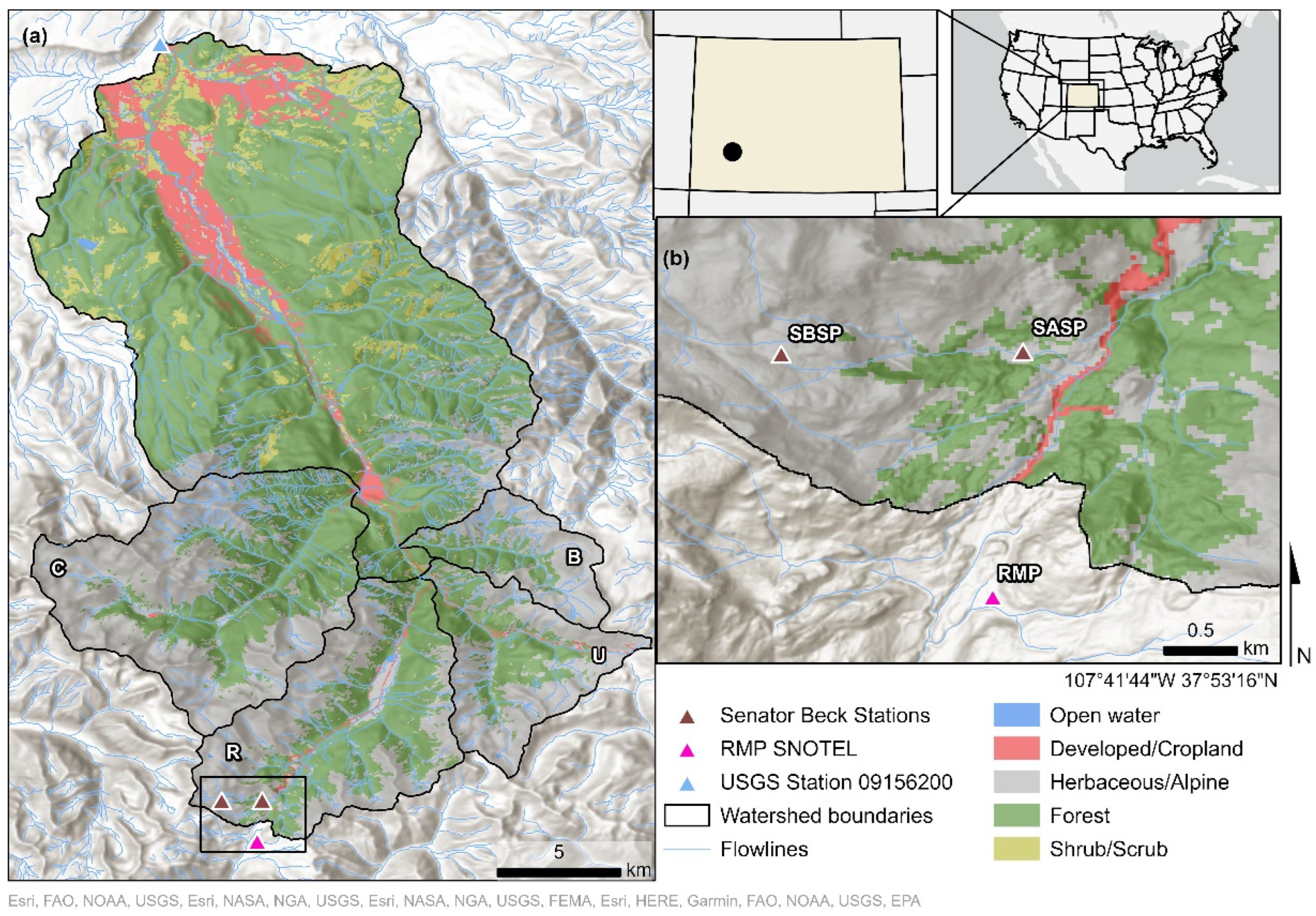
2.1. Study Area

The Uncompahgre River watershed in the southwestern Colorado San Juan Mountain range serves as a primary source of irrigation and drinking water for local communities and supplies the Ouray Hydrodam and Ridgway Reservoir (Figure 2). The snowpack within this watershed typically exhibits longer accumulation periods, lower peak SWE values, later melt onset dates, and lower melt rates than basins in other North American snow regimes [20]. This analysis targeted peak flow at the Uncompahgre River, which is the outflow point for the upper 386 km2 (13%) of the 2888 km2 Uncompahgre River basin (HUC 14020006), flowing into the Gunnison River (Figure 2a). As previously noted, hydrographs in the Uncompahgre typically exhibit two primary peaks (Figure 1 and Figure A1) after the initiation of melt in 18 of the 20 study years, suggesting that two distinct melt events occur in the persistent snow zones upstream of Uncompahgre River station (Figure 2). While the entire study basin is dominated by forested (or sub-alpine) land cover (~70%), the four seasonally snow-covered headwater sub-basins, i.e., Canyon Creek, Red Mountain Creek, Upper Uncompahgre River, and Bear Creek (Figure 2a), [21], are dominated by 55 to 70% alpine land cover (Table A1).
Two snow-monitoring stations, the Swamp Angel Study Plot (SASP) and the Senator Beck Study Plot (SBSP), fall within the Red Mountain Creek headwater basin, and the Red Mountain Pass (RMP) SNOTEL station falls just outside the basin boundary. This analysis uses the concurrent data record from these three datasets: streamflow, SWE at RMP SNOTEL station, and snow depth at SASP and SBSP (Table A2) for Water Year (WY) 2005 to 2024 (Figure 3). WY is the period from 1 October of the previous year to 30 September of the current year. SWE data were not available for the SBB (Swamp Angel Study Plot and Senator Beck Study Plot) sites. The study watershed ranges in elevation from 4315 m at the Mount Sneffels’ peak to 2096 m at the outlet, just upstream of Ridgway Reservoir. The area receives a mean of 823 mm of precipitation annually (USGS, <https://streamstats.usgs.gov>), most of which falls as snow [25].

2.2. Data Preparation

Daily streamflow data for the Uncompahgre River near Ridgway were retrieved from the U.S. Geological Survey [17]. From the hydrographs, peak streamflow amount and date were manually extracted for Peak 1 and Peak 2 based on their occurrence in time. For peaks to be considered distinct, streamflow values must have dropped to 70% of Peak 1, before increasing again. Initially, we employed a more restrictive threshold (e.g., 60%) but this failed to identify visually obvious Peak 2 events in five of the twenty years examined (e.g., Figure 1c). We excluded local streamflow peaks caused by summer monsoonal rains and early-winter snowmelt events by only considering peak flows that occurred after 80% of peak SWE and before 1 July. Although no major peak events occurred outside these parameters, specifying the date window considered in this analysis emphasizes the focus on snowmelt-driven peak runoff events. Three of the eighteen years examined exhibited three distinct peaks (Figure A1); here, the peaks exhibiting the two highest streamflow values were selected (Figure 3a). The two years with only one peak (2014 and 2021; Figure A1) were considered only when examining Peak 1.
Daily snow data were retrieved from the Center for Snow and Avalanche Studies [19], for SASP and SBSP, and from the Natural Resources Conservation Service [18] for RMP. Snowpack quantities and timing were extracted for peak snow amounts and dates (SWE from the RMP SNOTEL station and depth from CSAS stations), dates of 50% and 80% of peak snowpack after the onset of melt [4], and SDD [26,27,28] (Table A2). Note that SDD is called snow all gone (SAG) in some papers (e.g., [26,27,28]). Since peak SWE and peak depth can persist for more than one day during any given water year, the earliest date was selected to represent peak occurrence. Annually, there is only one day for 50% peak SWE or peak depth since it occurs during full snowmelt (Figure 4). SDD was calculated for each station as the first date after peak SWE at RMP, or peak snow depth at SBSP and SASP, when SWE or snow depth is zero.

2.3. Data Correlation

Peak streamflow dates were plotted against two primary snow-timing metrics (SDD and 50% of peak depth or SWE) at the three snow stations and visually inspected for proximity to a 1:1 line. The Nash–Sutcliffe efficiency (NSE) coefficient [29] and correlation coefficient (R2) were used to quantify the correlation fit [30] between observed peak flow and SDD. This region can have large dust-on-snow events [26,31], and such events seem to alter streamflow substantially [28,32]. The years 2009 and 2012 experienced the highest number of dust-on-snow events for the 2005–2019 period [27,28]. During the study period, 2012 was the driest year (lowest peak SWE) and yielded a different streamflow response when compared to average or high snow years [15]. Thus, the correlation was also considered without 2009 and 2012.
Three WYs (2005, 2011, and 2014) are used to highlight differences among years with similar peak flows (30.5 m3/s) but varying peak streamflow characteristics (Figure 1). For these three years, peak SWE amount varied from average (represented by 2014) to 40% snowier than average (2011) (Figure 3b and Figure 4). The timing of peak SWE (Figure 4a) and peak depth (Figure 4b) were similar for two years (2005 and 2014) and several weeks later in the snowier year (2011).

2.4. WRF-Snow Model SWE and SDD Distributions
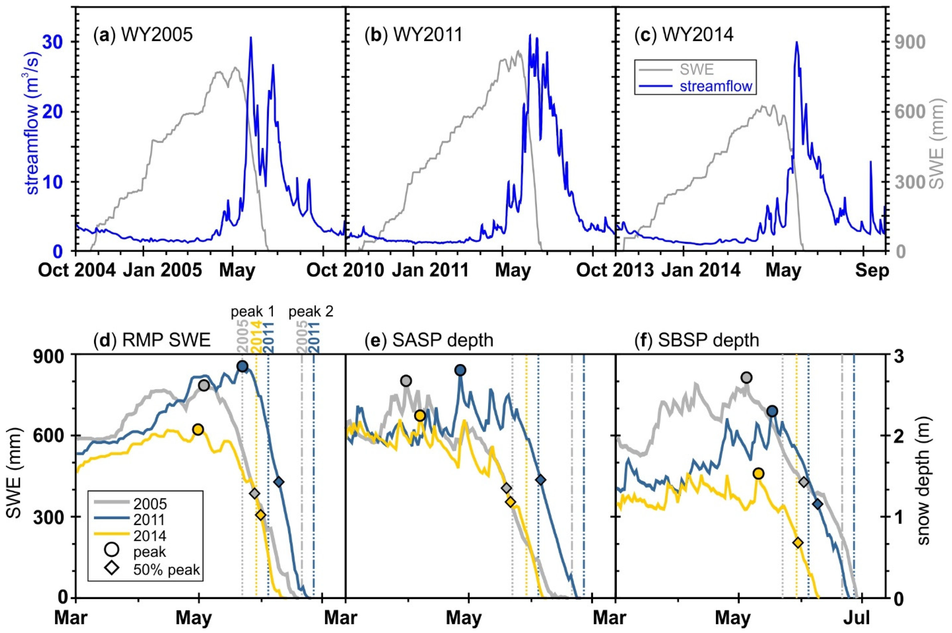
Since snowpack observations are only available at limited point locations, the second objective of this study was to estimate the spatial distribution of modeled peak SWE and SDD across forested and alpine regions within each of the four headwater watersheds to further understand the connection across the two ecozones and the twin-peak behavior. To this end, we use the Weather Research and Forecasting Model (WRF), a 4 km, convection-permitting dataset that models meteorological conditions from the recent past (WY 2001 to 2013) [33]. Hammond et al. [25] used WRF data to drive SnowModel at fine resolution (daily, 100 m) [34] to model snow conditions (SWE, solid precipitation, total precipitation, snowmelt, total runoff, and air temperature) in the Upper Colorado River Basin. The SWE variable was used to identify peak SWE, peak SWE date, and SDD at each grid cell in the four sub-basins. The resultant grids were analyzed in ArcGIS Pro (version 2.8.0) for the four sub-watersheds. Grids were further subset into alpine and forested regions within each watershed. Mean values for each area (entire watershed, alpine watershed region, forested watershed region) were calculated for each watershed and tested for statistical differences using Tukey’s Honest Significant Difference (Tukey’s HSD) method at a 95% confidence interval. Here, the focus WY 2014 was not investigated since WRF-SnowModel data are not available [25]. The cumulative area per sub-basin per land-cover type (forested versus alpine) was computed for April 15 using the clear-sky solar radiation tool in ArcGIS Pro (version 2.8.0) (Figure A2). We focused on 2005 and 2011 only, due to the data volume necessary for this investigation.

3. Results

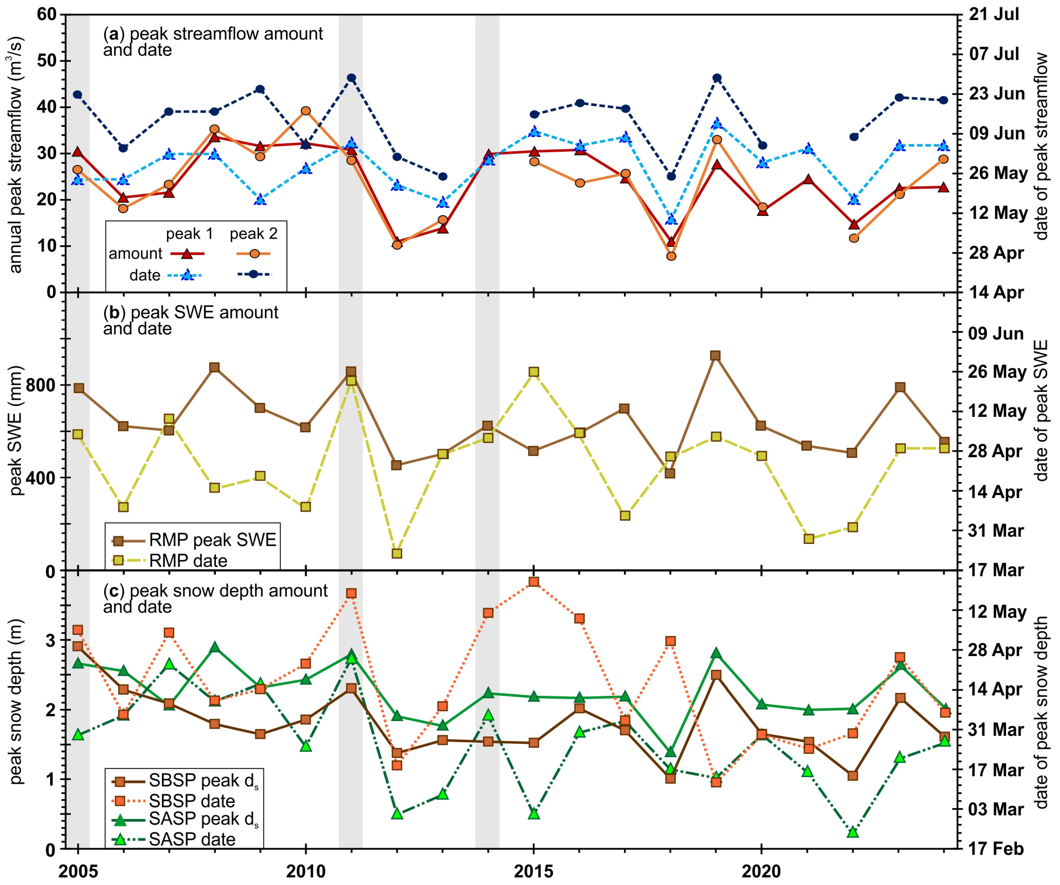
3.1. Peak 1 Streamflow Event

The timing of Peak 1 streamflow correlates better with SASP SDD (Figure 1a) than with SBSP SDD (Figure 1b) or RMP SDD (Figure 1c), based on both the correlation coefficients and the NSE values (Table 1). RMP SDD had the highest R2 values, but poorer NSE values. All NSE values illustrated that the correlations were not as good as using the mean observed value, i.e., all NSE values were negative. Removing the dustiest and lowest snow years (2009 and 2012) did not improve the correlation statistics. However, considering first streamflow peaks occurring before 15 June, the remaining 14 years for SASP has an R2 of 0.66 and an NSE of 0.58. The slope of the best fit line was less than one due to the later Peak 1 timing and much later SDD values. SDD at both SBSP and RMP occurred later than Peak 1 for all years except 2012 (Figure 4b,c). For SASP, SDD in 2005 and 2018 (the second shallowest snow year) occurred much later than Peak 1. At SBSP and RMP, 2005, 2018, and 2019 (deepest snow year) were all much later than Peak 1.
Peak 1 occurrence correlates better and has a stronger 1:1 fit with 50% peak depth date at SBSP and 50% peak SWE date at RMP (Figure 5b,c) than with SDD (Table 1). At SASP, the 50% peak depth date was well before Peak 1 (Figure 5a). When 2009 and 2012 were removed, all statistics improved, with SBSP and RMP being statistically satisfactory [30].

3.2. Peak 2 Streamflow Event

Except for the years 2018 and 2005, Peak 2 occurred later than SASP SDD with a maximum difference of 36 days in 2009 (Figure 4d). The correlation for SBSP SDD and Peak 2 was better (Figure 4e) than RMP (Figure 4f). The two outlier years (2009 and 2012) impacted SDD modeled fit (Table 1; Figure 4). Across all three stations, SDD in 2009 and 2012 occurred substantially earlier than the Peak 2 date (an average of 33 days for 2009 and 15 days for 2012), particularly compared to the mean (3 days earlier for RMP, 7 days earlier for SASP, and 1 day later for SBSP).
Peak 2 was also later than SDD at SASP and RMP in 2022 and 2024. At SBSP, 2022 was also substantially later (18 days), but not 2024. Peak 2 was 10 days earlier than SBSP SDD in 2019. For SBSP, if we consider the period from 23 May to the end of June (14 years), R2 improved to 0.92, NSE to 0.890, and the slope is 1.03.
Fifty percent of peak depth (at SASP and SBSP) or SWE (at RMP) occurred well before Peak 2 (Figure 5d–f). The largest difference was with the year 2009. Removing it and the lowest snow year (2012) improved the correlation statistics.

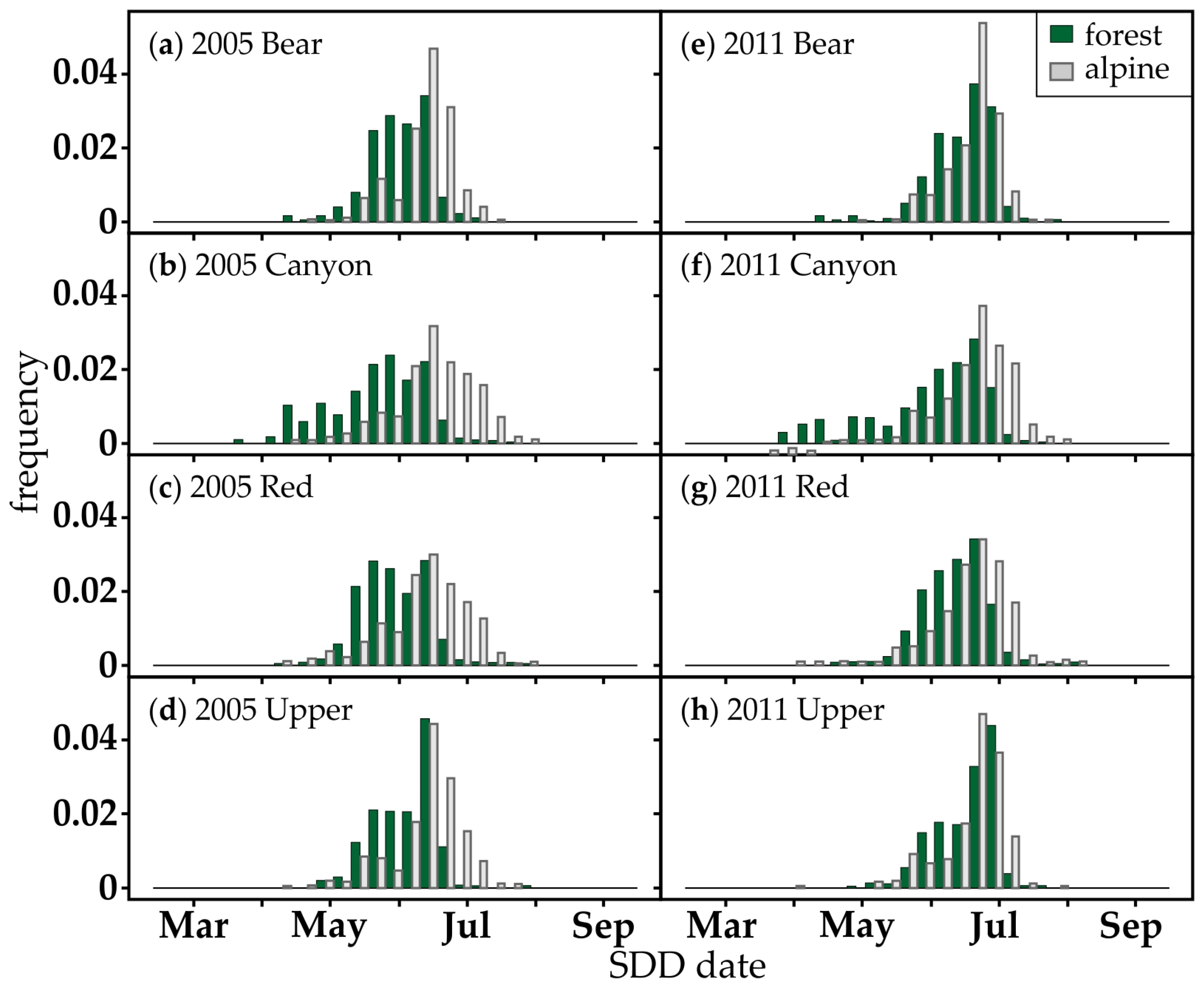
3.3. WRF-Snow Model SDD Distributions

Correlation results between snow metrics at alpine and forested snow-monitoring stations and peak streamflow events highlighted the nuance of these headwater persistent snow zones. To further explore the dynamics between region and peak streamflow occurrence, we zoom into the sub-watersheds nested in the Uncompahgre River’s headwater region. This portion of the analysis considers spatial variability in snowpack that point measurements at snow-monitoring stations do not capture. Across the four headwater watersheds examined, Canyon Creek experienced the longest melt-out period. The forest region exhibited the earliest mean SDD (27 May ± 18 days in 2005 and 5 June ± 22 days in 2011), while the alpine region exhibited the latest (mean SDD 25 June ± 16 days for 2005 and 29 June ± 14 days in 2011) (Figure 6, Table A3). This watershed is also the largest of the four sub-watersheds (Table A1). The other three watersheds seem to share similar distributions in SDD, with mean SDD in the forest ranging from 3 June (±12 days) in Red Mountain Creek to 7 June (±12 days) in the Upper watershed in 2005 and 14 June (±12 days) in Red Mountain Creek to 19 June (±12 days) in the Upper watershed in 2011. SDD in the alpine regions ranged from 21 June (±11 days) in Bear Creek to 23 June (±12 days) in Upper for 2005 and 27 June (±10 days) in Bear Creek to 29 June (±11 days) in Upper for 2011 (Figure 6, Table A3). Of these three watersheds, Red Mountain Creek is the largest and has the least alpine, while Bear Creek is only a third the size and has the greatest percentage of alpine (Table A1).
When mean SDD were compared across watersheds and regions, the only regions that exhibited no statistical difference across both 2005 and 2011 were (1) the alpine region of Red Mountain Creek and the alpine region of Bear Creek (p-value = 0.89) and (2) the forest region of Upper and the forest region of Bear Creek (p-value = 0.74). Considering mean SDD across entire watersheds (i.e., not divided by ecozone), Upper and Bear Creek exhibited no statistical difference (p-value = 0.84, 0.72 for 2005 and 2011, respectively).

4. Discussion

4.1. Correlations Between Peak Streamflow Date and Snowpack Measurement

This study suggests that simple snowpack metrics such as the snow disappearance date, and the date of 50% of peak depth or SWE, could provide a reasonable estimate of peak flow occurrences in the Uncompahgre River. Removing 2009 and 2012, Red Mountain Pass SNOTEL site metrics (50% maximum SWE date and SDD) were satisfactory predictors [30] for Peaks 1 and 2, respectively. SDD at Senator Beck Study Plot better explained Peak 2 occurrence, and 50% maximum depth date at SBSP was also successful in estimating Peak 1 occurrence. SDD was reasonably correlated with Peak 1 at Swamp Angel Study Plot, the forest site (Figure 4a). When removing 2009 and 2012, the slope became closer to 1; while NSE was poor, 50% of peak depth or SWE could be considered for forecasting the timing of Peak 2 (Table 1).
The SBSP station, representing the alpine ecozone, melted out before RMP in 5 out of the 20 years examined and at the same time as SASP in 3 out of the 20 years examined. While RMP is in the forest (Figure 2), SDD does not correspond to peak streamflow as consistently as SASP or SBSP. The relative locations of the individual stations is relevant, but due to the proximity of SASP and RMP (Figure) and the similar elevation, it would be expected that SDD should be quite similar. Also, 50% of peak SWE does not necessarily correspond to 50% of peak depth (Figure 1); at RMP, the former occurs on average 8.5 days later than the latter (range of 3 to 38 days) with an R2 of 0.62. Snow depth is easier to measure than SWE [35], especially over space [35]. Further, SWE is rarely measured in the alpine [18], yet a majority of this watershed is alpine (Table A2).
Melt-out dynamics in the two ecozones could partly dictate magnitude-based peak estimations (Figure 4 and Figure 5). All correlations addressed in this study rely on a time-based division of the two Uncompahgre River peak streamflow events. Peak flow events could also be organized based on relative magnitude (Figure A1), i.e., Peak 1 represents the largest peak flow event of the year. Organizing peak events based on date of occurrence is also comparatively more useful for water managers.
Examining water years 2009 and 2012 illustrates the additional importance of considering dust on snow events when forecasting runoff. These two water years had the highest number of dust-on-snow events for the 2005–2019 period [27,28] and exhibited melt-out dates 14 to 25 days earlier than the average SDD at each station. When using SDD to estimate Peak 2, these two years also significantly impacted R2 and NSE values. Water year 2012 also exhibited the lowest maximum streamflow and second-lowest maximum SWE value across the 20-year study period (11.0 m3/s and 452 mm, respectively) (Figure 3). However, water year 2018 exhibited similar peak streamflow and maximum SWE values and did affect the Peak 1 correlation but not Peak 2. The comparatively normal 2009 water year (Qmax = 31.7 m3/s; SWEmax = 699 mm) affects the correlation for both streamflow peaks. Deposited dust has previously been shown to decrease snow-cover duration and accelerate melt in Senator Beck Basin [26,27,28,31,32] and it is likely that these outlier years are better explained by dust on snow impacts than by snowpack and streamflow characteristics.
The relative success in using the Red Mountain Pass SWE data to estimate both the Peak 1 and Peak 2 streamflow events illustrates the potential for similar correlations in other high-elevation Colorado watersheds. Snow depth data are available for about half the recorded period at SNOTEL stations compared to SWE data collection; thus, SWE was used here to extend the study period. However, the results presented herein illustrate the importance of utilizing data collected in alpine ecozones, as metrics developed using the Senator Beck Study Plot depth data performed nearly as well as RMP in estimating the Peak 1 occurrence (NSE = 0.55 vs. 0.56) and better in estimating the Peak 2 occurrence (NSE = 0.67 vs. 0.49). SNOTEL sites are almost exclusively located in forest ecozones (at or lower than tree line) [18] and so simulate alpine snowpack accumulation, melt, and their subsequent impact on streamflow dynamics less reliably. In river basins that contain relatively large expanses of alpine like the Upper Uncompahgre (Figure 2 and Table A1), coupled monitoring sites in both the forest and alpine ecozones become more important. Although melt out in the forest (represented by SDD at SASP and RMP) is only a reasonable estimator of the Peak 1 occurrence, the melt out of alpine basins (represented by SDD at SBSP) is a better estimator of the occurrence of the Peak 2 streamflow event.

4.2. Modeled Peak SWE and SDD Across Space

The correlation between snow metrics and the twin-peak behavior observed in the Uncompahgre proves helpful for estimating peak streamflow occurrence but do not explain the mechanism behind this twin-peak behavior. A potential explanation is that this twin-peak behavior is driven by melt-out differences in headwater sub-watersheds. Responses were different at both the sub-watershed scale (Figure 2) and at the ecozone (alpine/forest) scale (Table A1). At the watershed scale, the Upper and Bear Creek watersheds seem to act as a single “melt-unit” while the Canyon Creek watershed appears to melt out more slowly than either this Upper/Bear group or Red Mountain Creek (Figure 6). The Upper and Bear Creek watersheds exhibited no statistical difference in mean SDD while the Canyon Creek watershed exhibited the most variability in SDD compared to other watersheds. These patterns in SDD distributions suggest that the Canyon Creek watershed melt-out occurs over a longer time, potentially driving the overall shape of the hydrograph, while the Upper/Bear Creek group corresponds to one peak streamflow event and Red Mountain Creek to the other. The Red Mountain Creek watershed is comparable in size to the Upper/Bear watershed combined group (Table A1). However, at a finer scale (i.e., alpine and forest regions within each watershed; Figure 6), this idea becomes more complicated and warrants further investigation. The only watershed regions to demonstrate no statistical difference in mean SDD were the (1) alpine regions of Red Mountain Creek watershed and Bear Creek watershed and (2) the forest regions of Upper and Bear Creek. This suggests that the persistent snow zone [21] in the Uncompahgre contains at least six distinct “melt-units”. Solar loading is different across the sub-watershed and between the forested and alpine ecozones, due to terrain differences (Figure A2). Twin-peak behavior has also been observed at the Senator Beck stream gauge (located in southern Red Mountain Creek), further supporting the need to examine headwater areas at both the watershed and ecozone scale.

4.3. Applications

For the purposes of estimating Peak 1 occurrence, explaining residual variation, and developing a simple linear model, 50% peak SWE and 50% peak depth were used as arbitrary markers for melt period. In higher-elevation Colorado basins, large spring precipitation events are not uncommon and can potentially sustain peak SWE, or close to peak SWE values, for several weeks before substantial melt begins [15,36]. The 50% maximum SWE date for RMP and 50% maximum depth for SASP and SBSP generally fall during the period of continuous, large-scale decreases in SWE, indicating substantial melt (Figure 4). For the purposes of estimating runoff timing, utilizing these metrics in place of true peak snowpack values reduces potential errors introduced by local increases in SWE and depth during spring storms. However, the date of the 50% peak (Figure 5) often falls after water managers have made allocation decisions.
Despite this, these results could prove useful as a forecasting tool. In 2012, the Natural Resource Conservation Service and the National Weather Service ceased coordinating their annual runoff forecasts, causing most western states to deliver on water rights claims using either the NRCS regression-based forecasts or the NWS River Forecast System’s hydrologic model [37]. These runoff-forecast models rely on temperature dependent snowmelt models that simplify the snowmelt process, producing variable and generally inconsistent streamflow results [38,39,40,41,42]. Changes in the snow-surface energy balance regime driven by climate change, dust-on-snow events, black carbon, and other forces could increase errors in forecasted runoff [26,31,41,43,44]. Basin-level forecast methods, like those employed by the Colorado Basin River Forecast Center, can also produce substantial errors when downscaling to smaller basins [45]. It is also important to note that water laws in many western states require that prior appropriation water rights contain specific time-of-year limitations. Several interstate compacts also revolve around spring calendar dates to some extent [46]. As those changes discussed above continue to alter when key streamflow events occur in western states, water right claims previously established during peak flows could be impacted. Developing alternative or supplemental forecasting methods, particularly for smaller basins, provides clearer information to water-resource managers as drought continues through the San Juan Mountain Range and the American Southwest [47,48].

4.4. Additional Factors Impacting Peaks 1 and 2

Another potential explanation or contributing factor could be differences in the rain/snow line associated with interannual variation in air temperatures during the melt season. A cooler spring melt season with a rain/snow line occurring at lower elevations may produce a single peak, while a warmer spring and associated rain/snow line at higher elevations may produce twin peaks. In the second instance, Peak 1 could be produced by accelerated melt driven by rain-on-snow events, while Peak 2 occurs once temperatures at higher elevations have reached melt. This follows similar logic to the forest/alpine hypothesis proposed here but allows for more interannual variability.
This study also illustrates a clear distinction in solar radiation values between alpine and forest ecozones (Figure A2) as well as distinct groups among the four headwater watersheds: the two largest watersheds (Red Mountain Creek watershed and Canyon Creek watershed) generally experience higher cumulative solar radiation values than their smaller counterparts (Bear Creek watershed and Upper watershed). This distribution gives further support for the split-ecozone hypothesis proposed initially. However, although it is apparent that more solar energy exists in the Upper Uncompahgre’s alpine ecozone, this region also exhibits much greater variations in snow depth than its forest counterpart, a pattern driven mainly by elevated wind exposure in alpine areas [49]. With this in mind, solar radiation distributions cannot fully describe melt patterns as any analysis completed using solely these values assumes an even distribution of snow depth. If combined with detailed snow depth raster datasets, such as the 3 m and 50 m raster datasets available for selected watersheds in California and Colorado [50], these distributions could provide a much clearer explanation for melt-out dynamics. However, no such data currently exists for the Uncompahgre basin.
We used a decrease of 70% of flow after Peak 1 to identify Peak 2. If this decrease was set at 60%, the second of the twin peaks could not be identified for WY 2010, 2015, 2016, 2017, and 2020. In those years, streamflow drops to 64, 69, 63, 65 and 66%, respectively, of Peak 1 before increasing to Peak 2.

4.5. Future Studies

We hypothesized that the timing of Peak 1 matches SDD in the forest and Peak 2 matches SDD in the alpine. This was true for most years. Peak 1 occurred within one week of SASP SDD for 13 of the 20 years (Figure 5a) with the two low snow years (2012 and 2018) being outliers and five high snow years with late peaks (see Figure 3a for peak date and Figure 3c for SASP SDD). Fifteen of the twenty Peak 2s occurred within 1 week of SBSP SDD (Figure 5e), with the outliers being the heavy dust year of 2009, the low snow year of 2012, and the two latest melt-outs of 2005 and 2019. The snow measurement stations are located on mostly flat terrain [26]. However, since there are many slopes and aspects across the areas (Figure A2), the variation in melt timing between N-NE-facing and S-SW-facing aspects could be explored further. Other studies have shown maximum snow accumulation and annual snowpack duration to be sensitive to changes in radiative forcing driven by changes in aspect, although none have attempted to correlate melt out on different aspects with peak streamflow [51,52]. Remote sensing can provide some additional data towards the spatial distribution of snow disappearance, including for the upper part of Red Mountain Creek [42,53], but either the spatial or temporal resolution may be too coarse.
A longer set of WRF runs (1981–2020) at the same 4 km resolution have been created for the conterminous United States [54]. These will likely be used to drive SnowModel [34], as per the runs used herein [25]. To reduce the computation effort, a coarser resolution (up to 500 m) could be used [55]. This twin-peaks phenomenon has been observed on other rivers [56], and such a spatial-modeling analysis [57] could address this in other systems. Snowpack data at 30 to 1000 m resolution are available for the Upper Uncompahgre River (at Ouray; USGS gauge 09146020) [58] which covers 52% of the watershed (Figure 2a) and most of the seasonally snow-covered area [21].

Author Contributions

Conceptualization, J.E.D., L.G.D., S.R.F., D.M.B., A.K.D.P. and W.E.S.; methodology, S.R.F. and L.G.D.; formal analysis, L.G.D. and S.R.F.; writing—original draft preparation, L.G.D. and S.R.F.; writing—review and editing, S.R.F., L.G.D., D.M.B., A.K.D.P., J.E.D. and W.E.S.; visualization, S.R.F. and L.G.D.; supervision, S.R.F.; project administration, S.R.F. All authors have read and agreed to the published version of the manuscript.

Funding

This research received no external funding.

Data Availability Statement

SNOTEL daily data for Red Mountain Pass (site 713) are collected by the Natural Resource Conservation Service Water and Climate Center [18]. Depth data for Senator Beck Basin study plots (Swamp Angel Study Plot and Senator Beck Study Plot) are collected by the Center for Snow and Avalanche Studies [19]. Daily streamflow data for the Uncompahgre near Ridgway, CO (USGS 09146200) can be found at U.S. Geological Survey [17]. WRF-SnowModel data were generated by Hammond et al. [25] and are available through the USGS at [58].

Acknowledgments

Many thanks to Stephanie Kampf and Elizabeth Tulanowski of Colorado State University (CSU) for their insight and support, and the CSU Honors Program for providing the opportunity to pursue this study. This author also acknowledges that this study site is located on traditional Núu-agha-tʉvʉ-pʉ̱ (Ute) and Pueblo lands <native-land.ca/>.

Conflicts of Interest

The authors declare no conflicts of interest.

Abbreviations

The following abbreviations are used in this manuscript:
CSASColorado Snow and Avalanche Center
ESRIEnvironmental Systems Research Institute
HUCHydrologic Unit Code
NRCSNational Resource and Conservation Service
NSENash–Sutcliffe Efficiency
NWSNational Weather Service
RMPRed Mountain Pass
SASPSwamp Angel Study Plot
SBBSenator Beck Basin
SBSPSenator Beck Study Plot
SDDsnow disappearance date
SNOTELSnowpack Telemetry
SWEsnow water equivalent
USGSUnited States Geological Service
WRFWeather Research and Forecasting Model

Appendix A. Station and Basin Data Summary

The appendix presents all hydrographs and SWE niveographs (Figure A1), the watershed characteristics used in WRF SnowModel analysis (Table A1), and a summary of peak SWE amount and date at the stations (Table A2). Presented for the sub-basins are the clear-sky solar radiation loading as function of cumulative area for the four sub-watersheds (Figure A2), and the summary statistics for WRF-SnowModel runs (Table A3).
Figure A1. Hydrographs for the 20 study years from the Uncompahgre River near Ridgway, Colorado (USGS station 09146200) gauge (blue) and SWE at Red Mountain Pass (gray) for (at) WY2005 through WY2024.
Water 17 02017 g0a1
Table A1. The characteristics of the entire study basin and the four headwater watersheds within the Uncompahgre basin. Data derived from the National Elevation Dataset (U.S. Geological Survey) [24] and the 2016 National Landcover Dataset (MRLC) [25].
WatershedArea (km2)Mean Elev. (m)Min. Elev. (m)Max. Elev. (m)% Alpine% Forest
Uncompahgre River Basin38628662096431569.130.9
Canyon Creek71.733242363431559.540.5
Red Mountain Creek55.233482590410954.445.6
Upper30.333362592409460.839.2
Bear Creek17.632892533403869.530.5
Table A2. Summary statistics for peak SWE amount and date at Red Mountain Pass SNOTEL (RMP), peak depth amount and date for Swamp Angel Study Plot (SASP) and Senator Beck Study Plot (SBSP), and snow disappearance date (SDD) at all three stations for WY 2005–2022.
Red Mountain Pass SNOTELSwamp Angel SPSenator Beck SP
snow-all-gone
mean7 June6 June12 June
standard deviation (days)141314
range (days)554158
peak SWE/depth amount (mm/m)
mean (mm/m)6352.251.79
standard deviation (mm/m)1470.400.49
range (mm/m)5081.521.92
peak SWE/depth date
mean22 April25 March16 April
standard deviation (days)181822
range (days)646271
Figure A2. Clear-sky solar radiation loading as a function of cumulative area for the four study watersheds divided into forest and alpine ecozones.
Water 17 02017 g0a2
Table A3. Modeled snow disappearance date (SDD) summary statistics in alpine and subalpine regions within four headwater watersheds of the Uncompahgre River basin for water years 2005 and 2011.
WatershedRegion20052011
Mean SDDSDD Range (Days)Mean SDDSDD Range (Days)
Canyon CreekAlpine25 Jun ± 16 days13229 Jun ± 14 days157
Forest27 May ± 18 days1105 Jun ± 22 days131
Red Mountain CreekAlpine22 Jun ± 15 days9327 Jun ± 13 days97
Forest3 Jun ± 12 days9314 Jun ± 12 days97
UpperAlpine23 Jun ±12 days8429 Jun ± 11 days79
Forest7 Jun ±12 days8519 Jun ± 12 days91
Bear CreekAlpine21 Jun ± 11 days7827 Jun ± 10 days125
Forest6 Jun ± 12 days7818 Jun ± 13 days87

References

  1. Barnett, T.P.; Adam, J.C.; Lettenmaier, D.P. Potential Impacts of a Warming Climate on Water Availability in Snow-Dominated Regions. Nature 2005, 438, 303–309. [Google Scholar] [CrossRef] [PubMed]
  2. Dozier, J.; Bair, E.H.; Davis, R.E. Estimating the Spatial Distribution of Snow Water Equivalent in the World’s Mountains. WIREs Water 2016, 3, 461–474. [Google Scholar] [CrossRef]
  3. Serreze, M.C.; Clark, M.P.; Armstrong, R.L.; McGinnis, D.A.; Pulwarty, R.S. Characteristics of the Western United States Snowpack from Snowpack Telemetry (SNOTEL) Data. Water Resour. Res. 1999, 35, 2145–2160. [Google Scholar] [CrossRef]
  4. Clow, D.W. Changes in the Timing of Snowmelt and Streamflow in Colorado: A Response to Recent Warming. J. Clim. 2010, 23, 2293–2306. [Google Scholar] [CrossRef]
  5. Stewart, I.T.; Cayan, D.R.; Dettinger, M.D. Changes toward Earlier Streamflow Timing across Western North America. J. Clim. 2005, 18, 1136–1155. [Google Scholar] [CrossRef]
  6. Stewart, I.T.; Cayan, D.R.; Dettinger, M.D. Changes in snowmelt runoff timing in western North America under a business as usual climate change scenario. Clim. Change 2004, 62, 217–232. [Google Scholar] [CrossRef]
  7. Knowles, N.; Dettinger, M.D.; Cayan, D.R. Trends in Snowfall versus Rainfall in the Western United States. J. Clim. 2006, 19, 4545–4559. [Google Scholar] [CrossRef]
  8. Fassnacht, S.R.; López-Moreno, J.I. Patterns of Trends in Niveograph Characteristics across the Western United States from Snow Telemetry Data. Front. Earth Sci. 2020, 14, 315–325. [Google Scholar] [CrossRef]
  9. Brown, R.D. Northern Hemisphere Snow Cover Variability and Change, 1915–1997. J. Clim. 2000, 13, 2339–2355. [Google Scholar] [CrossRef]
  10. Kunkel, K.E.; Robinson, D.A.; Champion, S.; Yin, X.; Estilow, T.; Frankson, R.M. Trends and Extremes in Northern Hemisphere Snow Characteristics. Curr. Clim. Chang. Rep. 2016, 2, 65–73. [Google Scholar] [CrossRef]
  11. Musselman, K.N.; Clark, M.P.; Liu, C.; Ikeda, K.; Rasmussen, R. Slower Snowmelt in a Warmer World. Nat. Clim. Chang. 2017, 7, 214–219. [Google Scholar] [CrossRef]
  12. Pfohl, A.K.D.; Fassnacht, S.R. Evaluating Methods of Streamflow Timing to Approximate Snowmelt Contribution in High-Elevation Mountain Watersheds. Hydrology 2023, 10, 75. [Google Scholar] [CrossRef]
  13. Uncompahgre Watershed Partnership. Uncompahgre Watershed Plan. Available online: https://www.uncompahgrewatershed.org/reports-plans/ (accessed on 24 May 2025).
  14. Fassnacht, S.R. Upper versus Lower Colorado River Sub-basin Streamflow: Characteristics, Runoff Estimation and Model Simulation. Hydrol. Process. 2006, 20, 2187–2205. [Google Scholar] [CrossRef]
  15. Fassnacht, S.R.; Deitemeyer, D.C.; Venable, N.B.H. Capitalizing on the Daily Time Step of Snow Telemetry Data to Model the Snowmelt Components of the Hydrograph for Small Watersheds. Hydrol. Process. 2014, 28, 4654–4668. [Google Scholar] [CrossRef]
  16. Sheeder, S.A.; Ross, J.D.; Carlson, T.N. Dual Urban and Rural Hydrograph Signals in Three Small Watersheds. J. Am. Water Resour. Assoc. 2002, 38, 1027–1040. [Google Scholar] [CrossRef]
  17. U.S. Geological Survey. USGS Water Data for the Nation. Available online: https://waterdata.usgs.gov/nwis/ (accessed on 24 May 2025).
  18. Natural Resources Conservation Service. Natural Resources Conservation Service—U.S. Department of Agriculture. Available online: https://www.nrcs.usda.gov (accessed on 24 May 2025).
  19. Center for Snow and Avalanche Studies. The Center for Snow & Avalanche Studies. Available online: https://www.snowstudies.org (accessed on 24 May 2025).
  20. Trujillo, E.; Molotch, N.P. Snowpack Regimes of the Western United States. Water Resour. Res. 2014, 50, 5611–5623. [Google Scholar] [CrossRef]
  21. Hammond, J.C.; Saavedra, F.A.; Kampf, S.K. Global Snow Zone Maps and Trends in Snow Persistence 2001–2016. Intl. J. Climatol. 2018, 38, 4369–4383. [Google Scholar] [CrossRef]
  22. ESRI. ArcGIS Hub. Available online: https://hub.arcgis.com/datasets (accessed on 24 May 2025).
  23. U.S. Geological Survey. National Hydrography Dataset. Available online: http://nhd.usgs.gov (accessed on 24 May 2025).
  24. Multi-Resolution Land Characteristics Consortium. National Landcover Dataset. Available online: https://www.mrlc.gov/ (accessed on 24 May 2025).
  25. Hammond, J.C.; Sexstone, G.A.; Putman, A.L.; Barnhart, T.B.; Rey, D.M.; Driscoll, J.M.; Liston, G.E.; Rasmussen, K.L.; McGrath, D.; Fassnacht, S.R.; et al. High Resolution SnowModel Simulations Reveal Future Elevation-Dependent Snow Loss and Earlier, Flashier Surface Water Input for the Upper Colorado River Basin. Earth’s Future 2023, 11, e2022EF003092. [Google Scholar] [CrossRef]
  26. Skiles, S.M.; Painter, T.H.; Deems, J.S.; Bryant, A.C.; Landry, C.C. Dust Radiative Forcing in Snow of the Upper Colorado River Basin: 2. Interannual Variability in Radiative Forcing and Snowmelt Rates. Water Resour. Res. 2012, 48, 2012WR011986. [Google Scholar] [CrossRef]
  27. Duncan, C.R. Patterns of Dust-Enhanced Absorbed Energy and Shifts in Melt Timing for Snow of Southwestern Colorado. Master’s Thesis, Colorado State University, Fort Collins, CO, USA, 2020. Available online: https://hdl.handle.net/10217/211991 (accessed on 15 June 2025).
  28. Fassnacht, S.R.; Duncan, C.R.; Pfohl, A.K.D.; Webb, R.W.; Derry, J.E.; Sanford, W.E.; Reimanis, D.C.; Doskocil, L.G. Drivers of Dust-Enhanced Snowpack Melt-Out and Streamflow Timing. Hydrology 2022, 9, 47. [Google Scholar] [CrossRef]
  29. Nash, J.E.; Sutcliffe, J.V. River Flow Forecasting through Conceptual Models Part I—A Discussion of Principles. J. Hydrol. 1970, 10, 282–290. [Google Scholar] [CrossRef]
  30. Moriasi, D.N.; Arnold, J.G.; Van Liew, M.W.; Bingner, R.L.; Harmel, R.D.; Veith, T.L. Model Evaluation Guidelines for Systematic Quantification of Accuracy in Watershed Simulations. Trans. ASABE 2007, 50, 885–900. [Google Scholar] [CrossRef]
  31. Painter, T.H.; Barrett, A.P.; Landry, C.C.; Neff, J.C.; Cassidy, M.P.; Lawrence, C.R.; McBride, K.E.; Farmer, G.L. Impact of Disturbed Desert Soils on Duration of Mountain Snow Cover. Geophys. Res. Lett. 2007, 34, 2007GL030284. [Google Scholar] [CrossRef]
  32. Painter, T.H.; Skiles, S.M.; Deems, J.S.; Brandt, W.T.; Dozier, J. Variation in Rising Limb of Colorado River Snowmelt Runoff Hydrograph Controlled by Dust Radiative Forcing in Snow. Geophys. Res. Lett. 2018, 45, 797–808. [Google Scholar] [CrossRef]
  33. Liu, C.; Ikeda, K.; Rasmussen, R.; Barlage, M.; Newman, A.J.; Prein, A.F.; Chen, F.; Chen, L.; Clark, M.; Dai, A.; et al. Continental-scale convection-permitting modeling of the current and future climate of North America. Clim. Dyn. 2017, 49, 71–95. [Google Scholar] [CrossRef]
  34. Liston, G.E.; Elder, K. A Distributed Snow-Evolution Modeling System (SnowModel). J. Hydrometeorol. 2006, 7, 1259–1276. [Google Scholar] [CrossRef]
  35. López-Moreno, J.I.; Leppänen, L.; Luks, B.; Holko, L.; Picard, G.; Sanmiguel-Vallelado, A.; Alonso-González, E.; Finger, D.C.; Arslan, A.N.; Gillemot, K.; et al. Intercomparison of measurements of bulk snow density and water equivalent of snow cover with snow core samplers: Instrumental bias and variability induced by observers. Hydrol. Process. 2020, 34, 3120–3133. [Google Scholar] [CrossRef]
  36. Serreze, M.C.; Clark, M.P.; Frei, A. Characteristics of Large Snowfall Events in the Montane Western United States as Examined Using Snowpack Telemetry (SNOTEL) Data. Water Resour. Res. 2001, 37, 675–688. [Google Scholar] [CrossRef]
  37. Pagano, T.; Wood, A.; Werner, K.; Tama-Sweet, R. Western U.S. Water Supply Forecasting: A Tradition Evolves. EoS Trans. 2014, 95, 28–29. [Google Scholar] [CrossRef]
  38. Hock, R. Temperature Index Melt Modelling in Mountain Areas. J. Hydrol. 2003, 282, 104–115. [Google Scholar] [CrossRef]
  39. Hock, R. Glacier Melt: A Review of Processes and Their Modelling. Prog. Phys. Geogr. Earth Environ. 2005, 29, 362–391. [Google Scholar] [CrossRef]
  40. Franz, K.J.; Hogue, T.S.; Sorooshian, S. Operational Snow Modeling: Addressing the Challenges of an Energy Balance Model for National Weather Service Forecasts. J. Hydrol. 2008, 360, 48–66. [Google Scholar] [CrossRef]
  41. Bryant, A.C.; Painter, T.H.; Deems, J.S.; Bender, S.M. Impact of Dust Radiative Forcing in Snow on Accuracy of Operational Runoff Prediction in the Upper Colorado River Basin. Geophys. Res. Lett. 2013, 40, 3945–3949. [Google Scholar] [CrossRef]
  42. Follum, M.L.; Niemann, J.D.; Fassnacht, S.R. A Comparison of Snowmelt-derived Streamflow from Temperature-index and Modified-temperature-index Snow Models. Hydrol. Process. 2019, 33, 3030–3045. [Google Scholar] [CrossRef]
  43. Milly, P.C.D.; Betancourt, J.; Falkenmark, M.; Hirsch, R.M.; Kundzewicz, Z.W.; Lettenmaier, D.P.; Stouffer, R.J. Stationarity Is Dead: Whither Water Management? Science 2008, 319, 573–574. [Google Scholar] [CrossRef] [PubMed]
  44. Dozier, J. Mountain Hydrology, Snow Color, and the Fourth Paradigm. EoS Trans. 2011, 92, 373–374. [Google Scholar] [CrossRef]
  45. Pagano, T.C.; Garen, D.C. Integration of Climate Information and Forecasts into Western US Water Supply Forecasts. In Climate Variations, Climate Change, and Water Resources Engineering; Garbrecht, J.D., Piechota, T.C., Eds.; American Society of Civil Engineers: Reston, VA, USA, 2006; pp. 86–103. [Google Scholar]
  46. Kenney, D.; Klien, R.; Goemans, C.; Alvord, C.; Shapiro, J. The Impact of Earlier Spring Snowmelt on Water Rights and Administration: A Preliminary Overview of Issues and Circumstances in the Western States. Western Water Assessment, Boulder, CO. 2008. Available online: https://sciencepolicy.colorado.edu/admin/publication_files/resource-2715-2008.24.pdf (accessed on 15 June 2025).
  47. Cook, B.I.; Ault, T.R.; Smerdon, J.E. Unprecedented 21st Century Drought Risk in the American Southwest and Central Plains. Sci. Adv. 2015, 1, e1400082. [Google Scholar] [CrossRef] [PubMed]
  48. Williams, A.P.; Cook, E.R.; Smerdon, J.E.; Cook, B.I.; Abatzoglou, J.T.; Bolles, K.; Baek, S.H.; Badger, A.M.; Livneh, B. Large Contribution from Anthropogenic Warming to an Emerging North American Megadrought. Science 2020, 368, 314–318. [Google Scholar] [CrossRef]
  49. Sexstone, G.A.; Fassnacht, S.R.; López-Moreno, J.I.; Hiemstra, C.A. Subgrid Snow Depth Coefficient of Variation Spanning Alpine to Sub-Alpine Mountainous Terrain. CIG 2022, 48, 79–96. [Google Scholar] [CrossRef]
  50. Airborne Snow Observatory. Airborne Snow Observatory. Available online: https://www.airbornesnowobservatories.com (accessed on 24 June 2025).
  51. Jost, G.; Weiler, M.; Gluns, D.R.; Alila, Y. The Influence of Forest and Topography on Snow Accumulation and Melt at the Watershed-Scale. J. Hydrol. 2007, 347, 101–115. [Google Scholar] [CrossRef]
  52. López-Moreno, J.I.; Revuelto, J.; Gilaberte, M.; Morán-Tejeda, E.; Pons, M.; Jover, E.; Esteban, P.; García, C.; Pomeroy, J.W. The Effect of Slope Aspect on the Response of Snowpack to Climate Warming in the Pyrenees. Theor. Appl. Clim. 2014, 117, 207–219. [Google Scholar] [CrossRef]
  53. Follum, M.L.; Downer, C.W.; Niemann, J.D.; Roylance, S.M.; Vuyovich, C.M. A radiation-derived temperature-index snow routine for the GSSHA hydrologic model. J. Hydrol. 2015, 529, 723–736. [Google Scholar] [CrossRef]
  54. Rasmussen, R.M.; Chen, F.; Liu, C.H.; Ikeda, K.; Prein, A.; Kim, J.; Schneider, T.; Dai, A.; Gochis, D.; Dugger, A.; et al. CONUS404: The NCAR–USGS 4-km long-term regional hydroclimate reanalysis over the CONUS. Bull. Am. Meteorol. Soc. 2023, 104, E1382–E1408. [Google Scholar] [CrossRef]
  55. Barnhart, T.B.; Putman, A.L.; Heldmyer, A.J.; Rey, D.M.; Hammond, J.C.; Driscoll, J.M.; Sexstone, G.A. Evaluating distributed snow model resolution and meteorology parameterizations against streamflow observations: Finer is not always better. Water Resour. Res. 2024, 60, e2023WR035982. [Google Scholar] [CrossRef]
  56. Lynch, D. Falling. Track 11 on Soundtrack from Twin Peaks; Warner Bros.: Los Angeles, CA, USA, 1990. [Google Scholar]
  57. Heldmyer, A.; Barnhart, T.B.; Putman, A.L.; Hammond, J.C.; Rey, D.M.; Sexstone, G.A. SnowModel Simulations for the Fraser River, East River, and Senator Beck Basin, Colorado Using Multiple Spatial Resolutions and Meteorology Datasets [Dataset]; U.S. Geological Survey: Reston, VA, USA, 2024. [Google Scholar] [CrossRef]
  58. Sexstone, G.A.; Hammond, J.C.; Barnhart, T.B. High Resolution Current and Future Climate SnowModel Simulations in the Upper Colorado River; U.S. Geological Survey: Reston, VA, USA, 2023. [Google Scholar] [CrossRef]
Figure 1. Hydrographs for the Uncompahgre River near Ridgway, CO (USGS station 09146200) for (a) WY2005 representing two distinctive streamflow peaks, (b) WY 2011 representing two less distinctive streamflow peaks, and (c) WY 2014 representing one single streamflow peak. The daily SWE time series is illustrated in gray for each year. The time series for all 20 study years (2005 to 2024) are included in Figure A1. Snowpack data for the same years presenting (d) SWE at the Red Mountain Pass (RMP) SNOTEL station in the forest, (e) snow depth at the Swamp Angel Study Plot (SASP) in the forest, and (f) snow depth at the Senator Beck Study Plot (SBSP) in the alpine. Circles illustrate peak SWE and depth dates while diamonds illustrate 50% of peak SWE or depth dates. The timing of streamflow Peak 1 (dotted line) and 2 (dashed line with two dots) is denoted by color for each year. Data are from the U.S. Geological Survey [17], Natural Resources Conservation Service [18], and the Center for Snow and Avalanche Studies [19].
Water 17 02017 g001
Figure 2. (a) Location, landcover types, and headwater watersheds of the Upper Uncompahgre watershed (HUC 14020006) and (b) relevant snow and streamflow stations (Table A2). Headwater watersheds in order of appearance from left to right: Canyon Creek (C), Red Mountain Creek (R), Upper Uncompahgre River (U), and Bear Creek (B) (Table A1). Data retrieved from ESRI [22], the U.S. Geological Survey National Hydrography Dataset [23], and the 2016 National Landcover Dataset (Multi-Resolution Land Characteristics Consortium) [24]. The alpine areas are shown in gray and listed as Herbaceous/Alpine, and the forested are shown in gray.
Water 17 02017 g002
Figure 3. (a) Peak streamflow and peak streamflow date for water years 2005–2024 in the Uncompahgre near Ridgway (USGS 09146200) (b) peak snow water equivalent (SWE) and peak SWE date at Red Mountain Pass SNOTEL station (site 713), and (c) peak depth and peak depth date at Colorado Snow and Avalanche Studies Swamp Angel Study Plot (SASP) and Senator Beck Study Plot (SBSP). WY 2005, 2011, and 2014 are highlighted in gray to illustrate the focus years. Data are from the U.S. Geological Survey [17], the Natural Resources Conservation Service [18], and the Center for Snow and Avalanche Studies [19].
Water 17 02017 g003
Figure 4. Correlation between snow disappearance date (SDD) at (a,d) Swamp Angel Study Plot (SASP; forested site), (b,e) Senator Beck Study Plot (SBSP; alpine site), and (c,f) Red Mountain Pass SNOTEL station 713 (RMP; forested site) versus the Peak 1 and Peak 2 flow event timing on the Uncompahgre River near Ridgway, CO (USGS 09146200). Linear fit statistics (R2 and Nash–Sutcliffe Efficiency, NSE values) are provided for all data (20 years for Peak 1) and with 2009 and 2012 omitted.
Water 17 02017 g004
Figure 5. Correlation between the timing of 50% peak depth at the Swamp Angel Study Plot (SASP), 50% peak depth at the Senator Beck Study Plot (SBSP), and 50% of peak SWE at the Red Mountain Pass SNOTEL station 713 (RMP) with the Peak 1 (ac) and Peak 2 (df) flow events on the Uncompahgre River near Ridgway, Colorado (USGS 09146200).
Water 17 02017 g005
Figure 6. WRF-SnowModel snow disappearance date (SDD) distributions in alpine and forest regions within four headwater watersheds of the Uncompahgre River basin for water years 2005 and 2011. Data derived from Hammond et al. [26].
Water 17 02017 g006
Table 1. Correlation coefficient (R2), Nash–Sutcliffe efficiency (NSE), and slope between snowpack variables (snow disappearance date or SDD, and date of 50% of peak SWE/depth) with peak streamflow dates at Uncompahgre River near Ridgway USGS gauging station (Peak 1 and Peak 2). Values in bold and italics indicate scenarios where snowpack variables were found to be satisfactory [30] predictors of peak streamflow.
LocationSnow VariableStatisticPeak 1: All2009&2012 RemovedPeak 2: All2009&2012 Removed
SASPSDDR20.590.560.550.74
NSE−0.21−0.32−0.580.13
slope0.5340.5580.5760.721
50% of peak depthR20.530.530.530.53
NSE−2.89−2.67−7.91−4.64
slope0.5750.6230.7010.849
SBSPSDDR20.640.600.470.77
NSE−2.00−2.480.040.67
slope0.5400.5830.5200.744
50% of peak depthR20.770.750.770.75
NSE0.460.55−2.880.31
slope0.6690.7050.5800.744
RMPSDDR20.670.650.540.71
NSE−0.72−0.940.010.49
slope0.6050.6300.6110.742
50% of peak depthR20.800.810.800.81
NSE0.400.56−3.210.32
slope0.7230.7910.6600.833
Disclaimer/Publisher’s Note: The statements, opinions and data contained in all publications are solely those of the individual author(s) and contributor(s) and not of MDPI and/or the editor(s). MDPI and/or the editor(s) disclaim responsibility for any injury to people or property resulting from any ideas, methods, instructions or products referred to in the content.

