Abstract
Groundwater plays an important role in areas facing water scarcity, which can cause many problems if poorly managed. In Northern Cyprus, in the Güzelyurt region, where agriculture is thriving, excessive and inappropriate groundwater use has caused a sharp decrease in water levels and electrical conductivity in many coastal areas. This study explores this problem using system dynamics tools designed to analyze feedback loops and causal links. The qualitative system dynamics approach is employed to investigate complex systems by focusing on structural and behavioral patterns through qualitative elements such as feedback loops, causal relationships, and system archetypes, rather than relying solely on numerical data. For this purpose, group model building is used, for which a basic model is built using library studies, and then the model is developed and improved through numerous interviews and meetings held with policymakers, farmers, soil and water managers, university professors, and representatives from the local community. The study examines water management practices, including transferring water from Turkey to Northern Cyprus and allocating a portion for agricultural use in Güzelyurt. It also explores agricultural strategies and the employment of advanced irrigation methods. In the tourism and urban consumption sectors, raising public awareness and educating citizens about water scarcity linked to climate change are highlighted as essential measures in promoting sustainable water usage.
1. Introduction
Water scarcity has become one of the major problems in the world today due to population growth and lifestyle changes, on the one hand, and issues such as climate change, on the other [1]. Climate change in arid and semi-arid regions significantly impacts water resource management [2]. In the context of water scarcity, water resource management, from transboundary waters to groundwater, is one of the fundamental pillars of all human societies [3,4]. Water resource and groundwater resource management can involve the management of their quantities or quality [5,6,7]. Groundwater resource management in urban areas is more prominent when its improper management causes serious problems, such as land subsidence and damage to urban infrastructure [8]. Therefore, groundwater resource management is of great importance, but systematic methods with a systemic perspective should be used due to the complexity of this issue.
To achieve the above-mentioned goal, systems thinking and its tools, such as system dynamics (SD), are useful and have been widely used for urban water resource management [9,10,11,12]. SD tools, such as the qualitative SD approach (QSDA), causal loop diagrams (CLDs), and feedback loops, help to better identify the system structure and analyze it correctly. Because water resource management usually has many components, it would be difficult to deal with it linearly and conventionally, which would ultimately lead to misguidance and poor management [10,11]. However, by using SD tools, the entire system structure and the cause-and-effect relationships between components can be discovered, and better and more effective management can be performed [10,11]. There are also various tools to obtain a SD model, but one of the most effective ones, which is achieved with the help of the stakeholders themselves, is group model building (GMB) [13]. In this method, the stakeholders themselves express their opinions on the model, and the components applied are based on their thinking.
GMB emerged in the 1980s as an innovative approach in SD that actively involves stakeholders in the modeling process to enhance model relevance and achieve a shared understanding and group consensus. Unlike earlier practices of gathering information through interviews and meetings, GMB integrates participants directly into model development using structured methods [13]. Vennix et al. (1996) identified four key dimensions in designing a GMB process: problem definition, the level of process structure, the type of model, and the project initiation method [14].
In this study, to properly analyze the management of groundwater resources in the Güzelyurt region of Northern Cyprus, the tools of systems thinking and the SD method are used. First, the theatrical background of the study is explained, which includes systems thinking, feedback loops, SD, QSDA, CLDs, and system archetypes. Then, the study area is introduced. After this, in the Materials and Methods section, GMB and the iceberg model are each first explained in general terms, followed by how they are used in the present study. Finally, in the Results and Discussion, regarding the urban sector and agricultural sector, the models built by GMB are analyzed; then, regarding the strategies and iceberg model, the strategies and solutions are introduced and analyzed. While previous research usually introduces the constructed model using the GMB method, the present study attempts to introduce and analyze strategies using another systems thinking tool.
2. Theoretical Background
In this section, an attempt is made to introduce systems thinking and its tools related to the present research to gain more insight into this issue, with an emphasis on water resource management.
2.1. Systems Thinking
One of the fundamental pillars of a systems approach is a holistic view. This approach is based on the belief that the world is composed of interconnected components that interact with and influence each other. When several components act together in a reciprocal relationship and their influence leads to the emergence of a goal or phenomenon, a “whole” or “system” is formed [15].
In the real world, phenomena and transformations are the result of the interactions of the components and factors that compose a system. No factor alone and apart from other components can create significant change. Humans are also involved in such a network of interactions, where multiple factors, through mutual influence, create different developments [16].
In reality, components are constantly interacting; each component is influenced by others and itself influences other parts. This interconnectedness encompasses the entire universe. However, to analyze any phenomenon from a systems perspective, one must focus on a specific range of meaningful components and interactions—those that have a tangible impact on the phenomenon under study and create an understandable framework [15,16].
Finally, although all components of the world are in constant interaction, within the framework of a systems perspective, a system or “whole” is defined as a set whose components are interconnected and effective with each other to achieve a specific goal [15].
2.2. Feedback Loops
One of the fundamental concepts in systems thinking is the concept of a “closed loop” or “feedback loop”. This approach suggests that human actions or natural events occur in a cyclical and feedback-driven framework [15]. Figure 1 provides an overview of the feedback process. In this cycle, conditions in the real world lead to decisions by humans or nature. These decisions lead to actions that, in turn, change the conditions of the environment, and these changes affect subsequent decisions and behaviors [15]. In other words, human life and the environment around them flow through feedback loops—cycles in which there is a continuous interaction between actions and their impacts on the environment [15]. In nature, decision-making is based on fundamental laws, such as the laws of physics and chemistry. However, when humans are involved, the rules for decision-making are also determined by humans themselves. However, human decisions and actions are also shaped within the same feedback loops and in accordance with the surrounding conditions. Individuals make decisions based on information that they receive or sense from the world around them and then act accordingly. The results of these actions create changes in the real world that will themselves form the basis for new data and decisions [16].
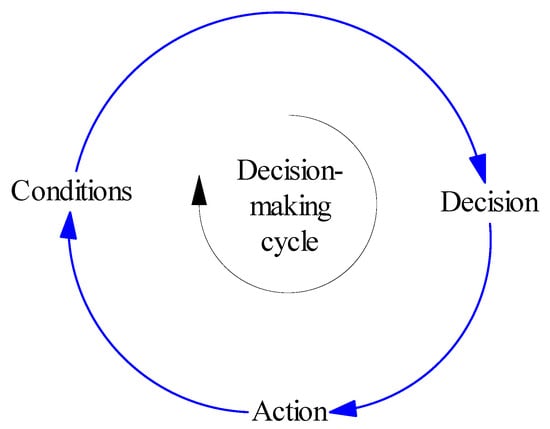
Figure 1.
Feedback loop in the real world.
This type of thinking, which is based on a closed loop, is opposed to a linear or one-way (open loop) approach, where cause-and-effect relationships are analyzed without considering feedback. In reality, different types of feedback play a fundamental role in the formation of phenomena [15,16]. Therefore, paying attention to this feedback can lead to more accurate and effective decisions to manage phenomena and create desirable changes in the real world. Although understanding and analyzing feedback is a difficult process, it can increase the validity of decision-making. However, it should be noted that direct feedback usually leads to other indirect feedback, the analysis of which is of great importance [15].
2.3. System Dynamics
In the context of this study, the most important element of systems thinking is the dynamic perspective. Based on this perspective, humans perceive the world as an ever-changing environment, a world in which change is constant [15]. This dynamism can be recognized through the transformations observed in various aspects of reality. Even the apparent stability of phenomena over a certain period of time can be considered a type of change [15].
The dynamic perspective is in contrast to the static perspective. The static approach examines the world at a specific moment and attempts to understand the relationships that prevail at that moment. This type of perspective focuses more on events that occur at a specific time and seeks to find the factors that led to the occurrence of an event in this specific period of time. Such a focus is usually reaction-oriented—that is, humans react to it after the event occurs [15].
Although identifying and managing events is necessary, it is not sufficient alone because the root cause of the problem may be ignored, and superficial measures may not only be ineffective but may even reinforce the problem in the future, and similar phenomena, but with wider dimensions, may be repeated [16].
In fact, events are often based on and are considered part of long-term trends. Therefore, in systems thinking, it is not enough to focus solely on events—attention must be paid to the more general flows and trends that contain events. In the framework of a dynamic approach, an event is only one component of the path of change over time, and the goal is to understand and analyze the factors affecting these changes [15].
The importance of paying attention to long-term trends stems from the fact that it enables an awareness of gradual and sometimes hidden threats—threats that, if ignored, can seriously damage the foundations of a system. This awareness allows measures to be taken to deal with these seemingly minor trends before they lead to the collapse or decline of the system [15].
In such situations, SD comes into play, which itself includes tools such as the QSDA, CLDs, and feedback loops, which are mentioned below.
2.4. Qualitative System Dynamics Approach
When a model is designed to analyze and understand a phenomenon with a systems approach, it is necessary to clearly display the model structure in the process of its construction and evolution [17]. This display helps to improve the design and development of the model and facilitates the process of understanding the phenomenon; as a result, it provides the possibility of examination, revision, and criticism [17]. Systems that are analyzed based on the theory of systems structure can be displayed in different ways [18]. Each of these display methods is applied at a specific stage of model development and analysis. In a closed system, “feedback”, as one of the key elements, forms a chain of causal relationships. From this perspective, systems thinking is based on the principle of causality [17]. At the macro level, the structure of the system is considered the main factor in the manifestation of its behavior; in other words, the behavior of systems results from their internal structure. The structure of any system is composed of components that interact with each other, and a change in one component can cause a change in other components [17]. These interactions create a chain of causal relationships between the components of the system and lead to the formation of closed feedback loops [18]. These mutual relationships create mechanisms within the structure that cause the behavior of the system to change over time [18].
At the micro level, the principle of causality is based on the assumption that a change in a variable is the result of the effect of another variable or variables. In other words, no change occurs without a reason, and, for each change, an effect factor must be identified [17]. The QSDA is based on this principle of causality. In this approach, concepts such as causal relationships, causal loops, and feedback loops are introduced, all of which are based on cause-and-effect relationships [18].
To define a causal relationship, we can say that, if a change in factor A causes a change in factor B, assuming that other factors are constant, A is the cause and B is the effect. This type of relationship is usually shown with an arrow pointing from A to B, so that the beginning of the arrow indicates the cause and its end indicates the effect (Figure 2).
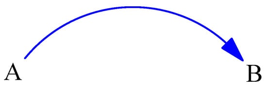
Figure 2.
Causal relationship.
For each cause-and-effect relationship, a logical explanation must be provided about its mechanism, and there must be empirical evidence to validate it [17]. When analyzing changes in the surrounding facts, it should be noted that the simultaneity or correlation of changes between two variables does not necessarily mean the existence of a causal relationship between them [17]. Similarity in the changes in two variables may be due to common causes and not a direct cause-and-effect relationship. Therefore, in causal relationships, the question must be answered as to why and how a change in the cause leads to a change in the effect. However, in correlation, only the simultaneity of changes is reported, without necessarily providing a reason for causality [18].
In causal relationships, when two factors, such as C and D, are positively related, any increase or decrease in C will cause a similar change in D. This type of relationship is indicated by a “+” sign on the arrow connecting C to D. In contrast, if there is a negative relationship between two factors, such as E and F, a change in E will cause the opposite change in F. This situation is represented by a “−” sign on the arrow between these two factors [17,18]. These concepts are illustrated in Figure 3.
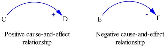
Figure 3.
Similar and opposite changes in causal relationship.
2.5. Causal Loop Diagrams
CLDs are used to represent causal loops. Causal loops are closed structures of cause-and-effect relationships in which the causal process begins with an agent and ultimately returns to the same agent, but this time as a consequence. In these types of structures, at least two elements simultaneously play the role of cause and effect [17]. For example, in Figure 4, two agents, A and B, are involved in a causal loop; A affects B and then B, in turn, affects A.
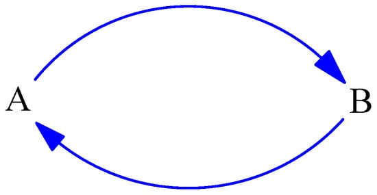
Figure 4.
Causal loop diagram.
In all causal loops, there is a two-way relationship between the agents. This relationship may be direct (only between the two agents) or indirect (with the involvement of intermediary elements) [17]. When the number of agents in the loop is more than two, the interactions are usually indirect [17]. In Figure 5, four agents, A, B, C, and D, are interdependent in the form of a loop; A affects B, B affects C, C affects D, and, finally, D affects A again.
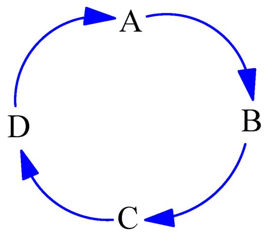
Figure 5.
Four interdependent agents in the form of a loop.
A positive causal loop occurs when a change in one element reinforces the same change in other elements of the loop [17]. These types of loops are represented by the symbol “+” or the letter “R” (an abbreviation for “reinforce”) (Figure 6). The operation of these loops usually leads to exponential growth over time.
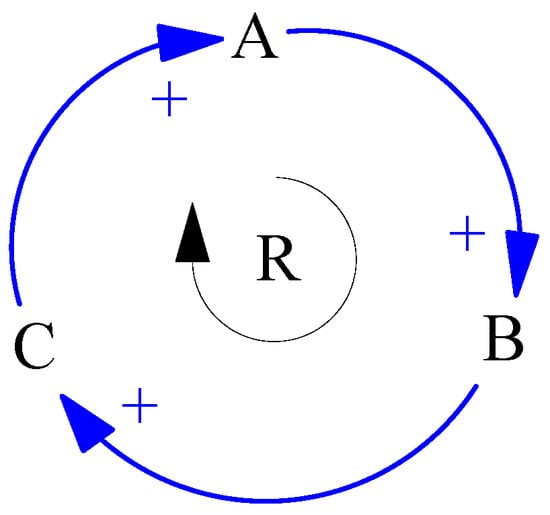
Figure 6.
A positive causal loop.
In contrast, a negative causal loop follows a mechanism that causes any change in one of the factors to be met with an opposing response in the other components [17]. These loops are represented by the symbol “−” or the letter “B” (an abbreviation for “balance”) (Figure 7). Sometimes known as “goal-oriented loops”, these loops tend to maintain stability and achieve a specific goal.
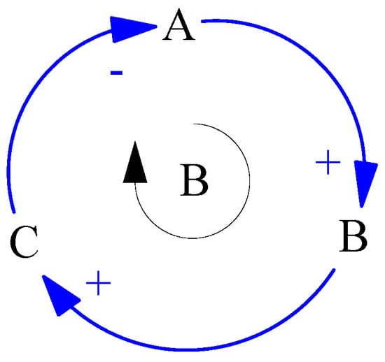
Figure 7.
A negative causal loop.
Most systems consist of a network of causal loops that are interconnected [18]. To accurately understand the dynamic behavior of a phenomenon and analyze the system related to it, the most important causal loops affecting its behavior must be identified [16,17,18]. At the beginning of the analysis process, these loops are selected based on initial dynamic hypotheses and are subsequently modified or supplemented with further investigation to obtain a comprehensive understanding of the system [17].
2.6. System Archetypes
In this section, some of the basic mechanisms that are common in the formation of dynamic phenomena are discussed. We know these mechanisms as “system archetypes”. These patterns are extracted with inspiration from various models developed in the field of SD and represent the main mechanisms of the emergence of some common events [19]. In practice, these fundamental mechanisms can activate other mechanisms tied to each situation’s specific conditions, requiring individual analysis [19]. Recognizing these simple patterns can be central to how feedback affects the changes in the surrounding environment [19]. Understanding the dynamics governing water resource systems would allow decision-makers to identify undesirable behaviors earlier and apply the necessary corrections promptly [20]. This will help to improve the planning and sustainable management of water resources. In the following, some practical examples of these system archetypes are presented to explain the challenges of water resource management.
2.6.1. Limits to Growth
A positive feedback loop alone can cause exponential growth, but, in the real world, no quantity can grow infinitely without limits [19]. The limits in the material world prevent the continuation of exponential growth. In this situation, a negative feedback loop acts as a controlling mechanism [19], which is generally as shown in Figure 8. In this model, feedback loop “A” is the factor that causes the growth of the system, while feedback loop “B” prevents further growth due to the lack of resources needed to feed and maintain the system. In the process of the negative feedback loop, as the current state of the system increases and the resources remain constant, the adequacy of the resources decreases. This decrease in the adequacy of resources, in turn, slows down the net growth rate. It should be noted that, in positive causality relationships, the change in the effect occurs in the direction of the change in the cause; therefore, as the adequacy of the resources decreases, its effect on net growth also decreases.
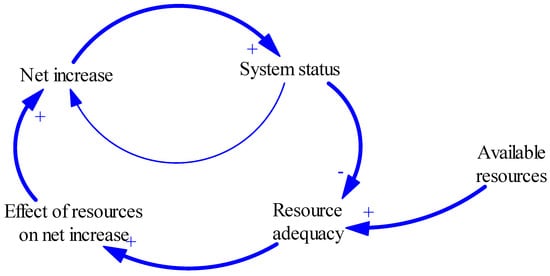
Figure 8.
The general mechanism of growth inhibition as negative feedback.
The dynamic behavior of an agricultural system that relies on groundwater for irrigation is an example of this archetype [20]. Figure 9 shows the CLD of the growth constraint archetype of this agricultural system. In this system, increasing agricultural activity increases the demand for irrigation water. In response to this demand, farmers expand the groundwater resources and increase the pumping rates, increasing their cultivation capacity and agricultural production (a reinforcing loop). However, the over-abstraction of groundwater resources sharply reduces the level of these resources, and, as a result, government regulations become stricter to limit groundwater withdrawals; this ultimately reduces the demand for groundwater (a balancing loop).
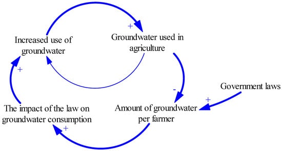
Figure 9.
The effects of government laws on groundwater consumption in agriculture.
2.6.2. Fixes That Backfire
One common system archetype in dealing with various problems is the tendency to choose temporary solutions instead of addressing fundamental solutions [19]. When individuals are faced with the symptoms of a problem, they often resort to methods that only temporarily alleviate them, without identifying and eliminating the root cause [19]. This type of superficial approach often exacerbates the problem in the long run and causes the problem to reoccur on a larger scale [20]. Figure 10 depicts the feedback loop patterns associated with this type of decision-making. Each visible sign of a problem usually originates from one or more root causes. The deeper the root of the problem, the more severe its symptoms will be. In such a situation, the individual has two paths.
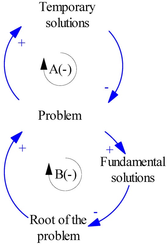
Figure 10.
General mechanism of “fixes that backfire”.
The first path is to resort to a temporary solution that aims to reduce the symptoms of the problem. In this path, the more severe the symptoms, the stronger the temporary measures taken to reduce the symptoms (negative feedback “A”).
The second path is to focus on finding and implementing a fundamental solution that directly targets the root of the problem (negative feedback “B”). In this approach, as the symptoms of the problem become larger, stronger fundamental solutions are considered, and, as the root causes are weakened, the symptoms gradually decrease or disappear.
The goal of both paths is to reduce the symptoms of the problem, but the main difference is that temporary solutions leave the root causes intact, while fundamental solutions deal with the root of the problem. The second path usually requires more time, deeper thought, and more effort to design, implement, and evaluate the results [19,20].
Ultimately, superficial solutions act as painkillers that only temporarily relieve the pain, while the underlying disease remains; meanwhile, fundamental solutions attempt to cure the disease completely.
Inter-basin water transfer projects often have unintended consequences, such as creating a false perception of water abundance and encouraging excessive development and population growth [21]. This situation can be explained by the “fixes that backfire” archetype. As shown in Figure 11, a severe water crisis encourages managers to implement water transfer projects to compensate for the existing shortage. This alleviates the problem in the short term, but, in the long term, the sustainable supply of water in areas facing resource shortages creates the false impression that further development is possible. As a result, increased population growth and greater development in these areas place more pressure on the water resources, ultimately exacerbating the water crisis, while the main resources continue to decline (side effects of the temporary solution).
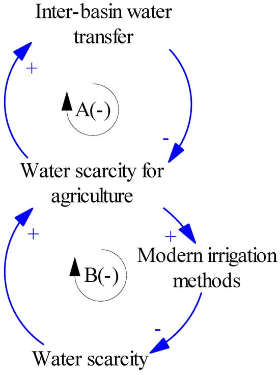
Figure 11.
“Fixes that backfire” for water scarcity in agriculture.
2.6.3. Side Effects of Temporary Solutions
As mentioned earlier, there are two general paths to addressing the symptoms of a problem: firstly, providing fundamental solutions to eliminate the root of the problem; secondly, using temporary solutions to deal with its symptoms [19]. As shown in Figure 12, two negative feedback loops (A and B) are activated to control the symptoms of the problem—one through temporary solutions and the other through fundamental solutions. In this section, the focus is on the unintended consequences of temporary solutions and their harmful effects.
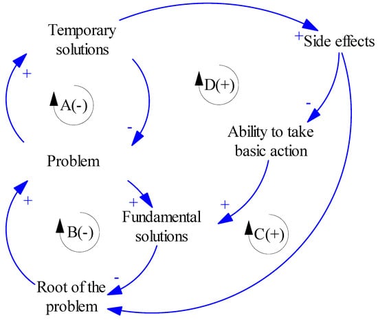
Figure 12.
General mechanism of side effects of temporary solutions.
In cases where temporary solutions cause side effects, the more intense these solutions are, the more severe the side effects will be [19]. As shown in Figure 12, these side effects can have two important consequences. First, these side effects may lead to the strengthening of the root of the problem. In such a case, the root of the problem is intensified, and, as a result, more temporary solutions are needed. This process, through the creation of positive feedback loop “C” in Figure 12, causes the symptoms of the problem to grow exponentially. The second consequence is that side effects can weaken the ability to implement basic measures. This reduction in capacity leads to a weakness in the implementation of basic solutions and disrupts the functioning of negative feedback loop “B”, which aims to eliminate the root of the problem. As a result, the root of the problem either remains unchanged or becomes more severe. This process creates positive feedback loop “D” in Figure 12, which further expands the symptoms of the problem.
For the problem of water scarcity and water shortages in agriculture, as explained in Section 2.6.2, migration from neighboring areas can be considered as one of the side effects of temporary solutions, as shown in Figure 13.
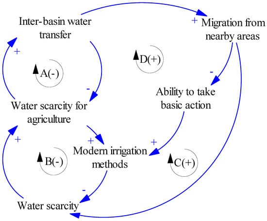
Figure 13.
Side effects of water scarcity in agriculture.
2.6.4. Success for the Successful
One of the most widely used system archetypes in the analysis of socioeconomic phenomena is the “success for the successful” archetype [19,20]. This archetype is activated when several activities or institutions compete with each other for access to limited and shared resources that are necessary for their progress [19]. In this competition, the institution that performs more successfully attracts more resources and support, while the competing institution or activity faces a decrease in resources and its performance is gradually weakened [19,20]. As a result, the gap between the successful and unsuccessful institutions increases over time. The main characteristic of this model is that one of the competitors is continuously improving, while the performance of the other is constantly declining [19].
The general cause-and-effect diagram of this model is shown in Figure 14. Suppose that two institutions, A and B, benefit from common resources. As A’s success increases, it obtains a larger share of the resources and consequently becomes more successful, while B’s success decreases.

Figure 14.
General mechanism of “success for the successful”.
This process creates a reinforcing loop, which is shown in Figure 15 as positive feedback loop 1.
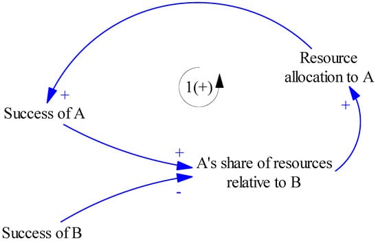
Figure 15.
One reinforcing loop due to “success for the successful”.
As A’s share grows, B’s share decreases and fewer resources are allocated to B. This reduction in resources causes B’s performance to fall further behind that of A, thus widening the achievement gap between the two entities. This process, which is shown in Figure 16 as positive feedback loop 2, causes B to increasingly lag behind A, effectively creating a downward cycle or negative feedback loop for B.
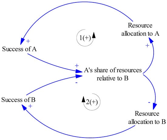
Figure 16.
Two reinforcing loops due to “success for the successful”.
The institutions mentioned earlier can be considered as water resource stakeholders [20]. In this regard, supply-based water resource management in a metropolitan area can be explained using the “success for the successful” model presented in Figure 17. In this model, the needs of a metropolis facing water shortages are prioritized over those of nearby sparsely populated areas [22]. As the metropolis increases its access to water resources, it becomes possible to develop further, and, as a result, its power to acquire additional resources increases. This process simultaneously limits the access of surrounding cities to water resources and weakens their development and competitiveness.
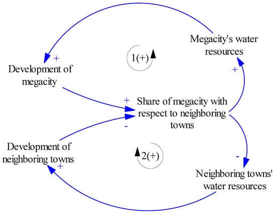
Figure 17.
“Success for the successful” in a megacity and its neighboring towns regarding water resources.
2.6.5. Tragedy of the Commons
The “tragedy of the commons” archetype occurs when different groups simultaneously use a limited resource, and each group consumes a larger portion of the resource to increase its growth [19]. This competition for greater exploitation causes the total consumption to exceed the available capacity of the resource, and, as a result, all groups face a shortage of resources [20]. This shortage leads to a decrease in the growth capacities of the groups, and the “tragedy of the commons” is formed. This tragedy is exacerbated when the overconsumption of the groups leads to the destruction of the resource itself [19,20].
The CLD in Figure 18 shows the overall situation of the consumption of a common resource by two groups. It is assumed that two groups, A and B, are engaged in an activity, such as fishing from a lake. Each group grows through a positive feedback loop: an increase in the capacity of group A increases its output, which is followed by further investment in capacity development. This investment again increases the capacity of the group, and the growth cycle continues. Group B acts similarly to Group A and increases its capacity through a similar feedback loop.
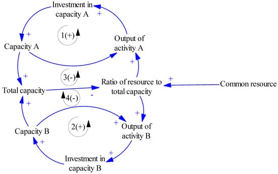
Figure 18.
General mechanism of “tragedy of the commons”.
The growth in the capacities of A and B increases the sum of the total capacity. However, since the amount of the resource (for example, the number of fish) is assumed to be constant, the increase in capacity reduces the ratio of the available resource to the total capacity. Initially, as long as this ratio is high, the activity of the groups is not affected. However, if the ratio of resources to capacity falls below a certain limit, the lack of resources directly affects the performance of the groups, and their production decreases. In this situation, the created capacities cannot be fully utilized, and the actual utilization of the available capacities will be lower than the predicted amount. As a result, the continuation of the activities of the groups may no longer be profitable and may even lead to the cessation of their activities. If the number of groups exceeds two, the pattern of competition and its consequences will intensify, creating a greater crisis for all groups.
Figure 19 also shows the cause-and-effect relationships in a case where the activities of the groups lead to a decrease in the resource. In this case, the increase in the activities of A and B increases the total amount of activities, and this increase accelerates the consumption of resources. As the resources decrease, the ratio of resources to capacity decreases, and, when the production capacities have reached their maximum, the resource shortage crisis intensifies. This crisis ultimately causes the collapse of the created capacities and the cessation of activities.
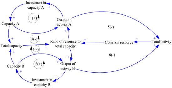
Figure 19.
“Tragedy of the commons” when a resource is depleted.
In water resource management, this system archetype emerges when multiple users share a common resource [20]. Suppose that two farmers rely on groundwater to irrigate their crops. If water withdrawals are made according to a regulated schedule, the resource can be more sustainable and the long-term benefits of the users can be optimized. However, in the absence of effective regulation, each farmer may withdraw water indiscriminately to maximize his short-term profits [20]. This situation is well described by the concept of the “tragedy of the commons” [23], in which each individual, by considering only his own interests, causes the deterioration of the common resource [24,25]. Figure 20 depicts a CLD diagram of this pattern in the context of groundwater exploitation, where two farmers (A and B) compete to maximize their net profits. Initially, the reinforcement loops, R1 and R2, allow the farmers to earn the desired profit. This process continues until a sharp drop in the groundwater level occurs, at which point the balancing loops, B1 and B2, dominate the system’s behavior. Eventually, the increase in pumping costs due to the drop in the water level reduces the profitability of each farmer.
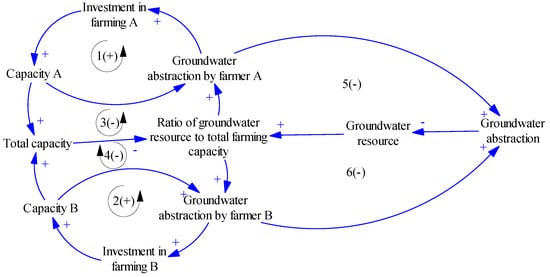
Figure 20.
“Tragedy of the commons” for two farmers.
3. Case Study
The Güzelyurt Basin is located in the northwest of Cyprus at the geographical coordinates (UTM) of 475000–507000 E and 3887000–3896000 N, at an average altitude of about 65 m above sea level. The population of this region is estimated to be about 30,037 people, and it has a semi-arid Mediterranean climate characterized by hot, dry summers and cold, wet winters. The annual rainfall is between 276 and 355 mm, the average air temperature is between 18.3 and 19.2 °C, and the relative humidity is about 68 to 71%. The Güzelyurt Plain, which is a gently sloping coastal plain, is mainly devoted to agriculture in its central part, and the terrain has a slope of close to 1% in most parts, except for the hills that extend from the northeast to the southwest of the region [26,27]. Figure 21 shows a map of the study area.
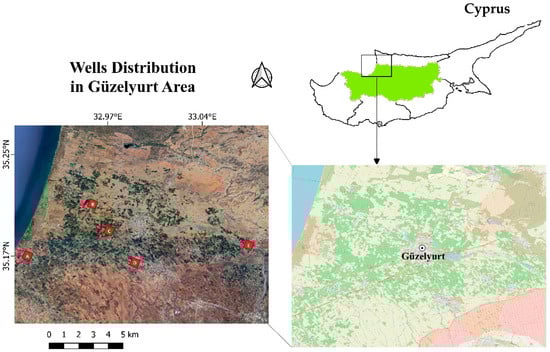
Figure 21.
Study area—Güzelyurt region and locations of selected wells.
Agriculture is the main economic activity in this region, with animal husbandry also common. Güzelyurt is particularly renowned for its citrus production, which meets the needs of the entire island, and this product has a significant contribution to the region’s exports and economy, providing about 40% of the island’s foreign exchange. In addition to citrus, other crops, such as melons, watermelons, strawberries, carrots, potatoes, mulberries, peppers, and eggplants, are also grown in the fertile soil of this plain [27]. In this region, the town of Güzelyurt and several surrounding villages are also located, which operate as tourist centers with local hotels. In addition, universities such as the Middle East Technical University of Cyprus (METU NCC) and the Cyprus University of Health and Social Sciences are located in this city and attract international students.
The Güzelyurt aquifer, which is a coastal open aquifer, faces challenges such as over-abstraction, saltwater intrusion, and regional and local pollution [28]. The aquifer is mainly composed of sand and gravel, with clay layers in some parts [29]. The soil of the region, which is classified as alluvial, is a mixture of sand, silt, and clay, with sand dominating. The upper layers of this soil are well drained, but this feature increases the vulnerability to saltwater intrusion [30] and pollution from local sewage [31]. However, the sandy texture of the soil provides good conditions for plant root ventilation.
Moreover, as can be seen in Figure 22 and Figure 23, the temperature has been increasing, with a gentle trend over a 13-year period, and the rainfall has decreased significantly over a 14-year period, which can be explained by climate change.
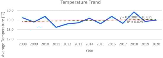
Figure 22.
Güzelyurt region’s temperature.
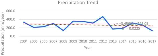
Figure 23.
Güzelyurt region’s precipitation (rainfall).
4. Materials and Methods
In this section, the research methods used—namely GMB and the iceberg model, both of which are systems thinking tools—are explained, and we then describe how they were applied in this research.
4.1. Group Model Building
GMB was first introduced in the 1980s by SD pioneers, including Richardson and Andersen (1995) [32], Richmond (1997) [33], and Vennix et al. (1996) [14]. These researchers recognized the potential for developing computer models and simulations with the participation of individuals who used SD modeling conventions [34]. Although there was a long tradition of using meetings and interviews to gather information about model structures, parameters, and policies in SD, GMB was a new step that aimed to directly involve individuals in the modeling process [35]. The fundamental principles of this approach emphasize the importance of involving stakeholders in model development—an action that is expected to not only lead to a more relevant model but also to promote a shared understanding, a group consensus, and motivation to implement the results [14,32].
Vennix (1996) has identified four main dimensions in designing a GMB process [14]. The first dimension concerns who defines the problem. In communities with limited experience in SD, this task is usually performed by an individual trained in the field. Secondly, group modeling projects are distinguished by whether the group process is structured or unstructured; in structured processes, a specific agenda is developed for the session, often in collaboration with the client or project sponsor, while unstructured processes rely on improvised group interactions and responses to the natural flow of conversation, and success in these processes requires a high level of expertise. The third dimension is the type of model sought. Some projects focus on creating informal causal maps that are used initially to conceptualize the system and define the problem or later to communicate the findings of the analysis. These maps alone are not considered the final output of the project unless they are accompanied by a formal simulation model [34]. Finally, the fourth dimension concerns how the project is initiated: does the process start from a “whiteboard” or is there an initial model structure? In the whiteboard approach, sessions begin with more freedom to explore issues and variables, whereas an initial conceptual model can serve as a starting point for the extraction of the causal structures of the system, especially in introducing participants to the language of SD [36].
As GMB methods have evolved, templates have emerged to guide small groups through the process of developing SD. Andersen and Richardson (1997) call these templates “GMB scripts” [37]. These scripts were originally standard exercises that teams used for activities such as determining group expectations (hopes and fears script), identifying problem variables (variable extraction script), discovering dynamic stories (timeline script), identifying causal structures (structure extraction script), introducing SD concepts (conceptual model script), and analyzing capacity–demand ratios (ratio script). Initially, these scripts were used as practical guides in designing and managing group modeling sessions without detailed documentation. Later, attempts were made to transform this process into a scientific framework [14,37], which emphasized the importance of recording sessions as a sequence of scripts [38], the development of ScriptsMap to map these sequences [39], and the systematic compilation of scripts in Scriptapedia [40]. In this framework, scripts play the role of templates in a template language [13].
One of the key ideas incorporated into the development of ScriptsMap and Scriptapedia was that, except for the initial scripts, each script takes the output of the previous script as input and produces a result for the next script. Another characteristic of scripts is that they generally fall into one of four categories of group activities [13]:
- Divergent activities to generate a range of ideas and interpretations;
- Convergent activities to cluster and organize these ideas;
- Evaluation activities to select or rank options;
- Presentation activities to educate participants or refresh their knowledge.
An important principle in designing modeling workshops is that sessions should alternate between divergent and convergent activities. It is also recommended that the results produced in one script be used in the next script to maintain coherence and efficiency across the process. This coherence can be considered as the efficiency of the sequence of scripts in the group modeling process [13].
For example, in the “graphs over time” script, participants draw and present stories about the dynamic trends of a problem. This divergent activity leads to the creation of a set of related variables. In addition to the graphs, stories with causal links are also shared. If both the data from the graphs and these causal stories are used in the subsequent script, participants will feel that their efforts have been worthwhile. Conversely, if only the list of variables is used and the causal stories are ignored, some of their efforts will go unused and a feeling of inefficiency may develop in the process [13].
4.2. Group Model Building in This Research
As previously stated, the involvement of stakeholders in the model development process increases the likelihood of the acceptance, trust, and use of the model [41]. Conversely, excluding some individuals from this process can lead to their resistance to the results [42]. Since an individual’s view of the system is limited to a specific domain, it is essential to consider all key actors [43].
Two methods were used to analyze stakeholders: firstly, brainstorming in a focus group session with experts [44,45]; secondly, using snowball sampling [44,46]. As explained by Reed (2009) [44], in the snowball method, initially identified individuals help to introduce new stakeholders. The use of these two methods was aimed at fostering the complete identification of stakeholders and avoiding the exclusion of important groups. Since stakeholder identification is a dynamic and iterative process [44], as the project progressed, more stakeholders were identified to increase the diversity and breadth of the network.
According to Hovmand (2014) [13], for group modeling workshops to be effective, the number of participants should be between 5 and 17; in our workshop, 12 people attended, including 3 policymakers, 3 farmers, 2 soil and water managers, 2 university professors, and 2 representatives from the local community of Güzelyurt (non-governmental organizations).
All participants received formal invitations, and their participation was without financial reward. None of the stakeholders had previous experience with SD techniques, although all were university-educated and many had master’s or doctoral degrees in their fields of expertise.
Individual semi-structured interviews were conducted to collect data. In this method, the questions and topics were predetermined, but the order and manner in which they were presented could be changed as needed to ensure that similar information was collected across all interviews. During each one- to two-hour interview session, each stakeholder actively participated in the development of an individual model, allowing them to observe, modify, or change components of the model in real time. At the end, each individual’s model was finalized with their own approval.
After the interviews were completed, the individual models were analyzed and merged to produce an initial qualitative model. This model provided a general understanding of the system’s behavior and reflected the stakeholders’ views. This step, which was a modification of the method of Vennix (1996) [42], aimed to establish a common ground and not to finalize the model. The initial model reflected the components that the majority of the stakeholders considered essential in understanding the system and was interpreted as a common ground. The model was also revised in a subsequent workshop to ensure that minority perspectives were also taken into account.
Following this, a GMB workshop was held, to which all identified stakeholders were invited. The workshop design was based on the four dimensions suggested by Hovmand (2014) [13]: (1) defining groundwater management in the case study area as the main issue; (2) structuring the workshop as a group; (3) setting goals to produce a shared model; and (4) starting work on a “whiteboard” basis. The organizing team consisted of a facilitator and two notetakers [32].
Given that presenting the initial model can weaken stakeholders’ sense of ownership, create bias, or impose mental framing [13,42], this model was not shown to the participants at the beginning. The workshop session proceeded as a discussion and was guided by the facilitator, during which components and relationships suggested by the stakeholders were added to the model. Any changes or additions to components were made only with the agreement of all attendees. This was a 6 h workshop with three 10 min breaks to gather the most information in the shortest time possible.
Modelers should extract causal structures using information provided by stakeholders and validate their models with archival data (such as previous studies, reports, laws, and statistical data), as well as personal experiences and observations [47]. In this study, a qualitative SD model was developed that represented the overall structure of the system based on the stakeholders’ opinions during the interviews, as well as data from the initial and group models. In the first step, the regional water balance was determined as the focus of the model, inspired by the work of Hassanzadeh et al. (2014) [48]. Then, the main causal structures in the initial and group models were identified and validated using other sources of information, including numerical and textual data. This cross-validation process was designed to prevent the introduction of incorrect data or structures into the final model. All data in the qualitative model could be traced back to previous studies, scientific sources, or field observations.
4.3. Stock–Flow Diagram and System Dynamics Modeling
Within systems thinking and SD, the state (stock) variable holds significance. State variables result from cumulative changes in other variables over time. In brief, they accumulate inputs and outputs over time. Flow (rate) variables closely relate to state variables. Input and output flows modify state variables. Flow variables are quantifiable over time. Both state and flow variables form the essence of a system’s structure. To simplify their connection, an auxiliary variable is introduced, derived from state variables, to elucidate their relationship. This leads to the creation of a stock–flow diagram (SFD), where formulas are incorporated into its variables [47]. Figure 24 depicts a simple SD model illustrated using an SFD incorporating a CLD.
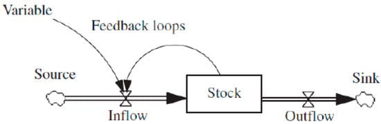
Figure 24.
Simple SD model illustrated using an SFD incorporating a CLD [17].
The system dynamics approach employs the quantitative simulation of all processes using rates. It distinguishes between two key types of variables: stocks and flows. Stocks represent a system’s present condition, shaped by past events, decisions, actions, and time delays. They evolve as flow rates either rise or fall. Flow variables directly influence stock variables and connect to the system’s inputs and outputs. Analyzing the disparities between inflows and outflows helps to determine if the stock is in a dynamic equilibrium [17]. The dynamics system is based on a general formula [17]:
in which “Inflows“ and “Outflows” represent input and output values at any time “s” between the initial moment “t0” and the current moment.
4.4. Iceberg Model
The image of an iceberg is a good example of how to analyze problems and find solutions (Figure 25) [49]. What is visible above the water surface represents the events and incidents that we experience in our daily lives. Meanwhile, the deeper layers that lie below the water line represent the structures and factors that shape these events. Systems thinking, using specific methods and habits, helps to uncover these deeper layers. The iceberg metaphor is a powerful tool in identifying and implementing fundamental changes in chronic problems.
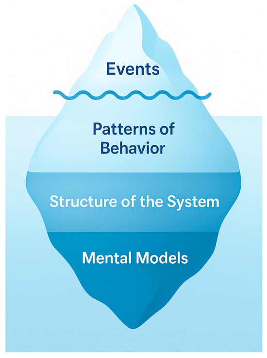
Figure 25.
Iceberg model.
Systems thinking tools can be used in different parts of the iceberg below the water surface. This model allows us to take a more holistic view of the system, rather than focusing solely on individual events [49].
The following is an explanation of how the different levels of the iceberg relate to some of the systems thinking tools [49,50].
- Patterns and Trends: Through behavior over time graphs (BOTG), we can analyze data and examine gradual changes. This tool helps us to better understand existing realities and trends and provides a framework within which to discuss how and why changes occur.
- Structure: Tools such as feedback loops, causal loops, and flow asset maps help us to explore the connections within the system and identify leverage points for effective change. Thinking at this level means examining the cause-and-effect relationships between system components.
- Mental Models: The ladder of inference clarifies individuals’ deeply held beliefs about the system. These models influence their perceptions of the current and future states. Since changing mental models is challenging, the ladder of inference tool helps to make these beliefs visible and analyzable.
4.5. Iceberg Model in This Research
Considering that the GMB applied in the present study, unlike most similar research, does not result in a cause-and-effect model, this study analyzes feasible strategies for better groundwater management in the study area. Considering the tools and capabilities of the iceberg model, this study attempts to construct an iceberg model to obtain feasible solutions and strategies after performing GMB, seeking to provide acceptable suggestions for stakeholders and policymakers.
5. Results and Discussion
In this section, GMB for groundwater resource management is explained. The cause-and-effect models are created separately for the urban and the agricultural sectors. Moreover, for each of the sectors, a preliminary model is obtained from the semi-structured interviews, and then a more evolved model is introduced as the main group model that was discussed in the workshop, and its structure is completed.
5.1. Urban Sector
The preliminary cause-and-effect model of groundwater management in the urban area of Güzelyurt is based on structured semi-structured interviews and the results obtained from them, with a greater emphasis on population growth and urban development, pressure on resources and damage to the environment, the pollution of groundwater resources, the role of groundwater management, and negative feedback from inefficient management. This model is shown in Figure 26.
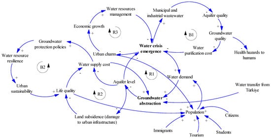
Figure 26.
The preliminary model of groundwater management in the urban sector.
As can be seen from Figure 26, this model has three reinforcing feedback loops and two balancing feedback loops. In reinforcing feedback loop 1, the water demand affects groundwater abstraction (similarly); groundwater abstraction affects the aquifer level (oppositely); aquifer level change affects water crisis emergence (oppositely); and, finally, water crisis emergence affects the water demand (similarly). Meanwhile, the population, which consists of citizens, students, tourists, and migrants (from rural to urban areas), affects the water demand (similarly), and the aquifer level affects the cost of the water supply (oppositely).
In reinforcing feedback loop 2, groundwater abstraction affects the aquifer level (oppositely); the aquifer level affects land subsidence (damage to urban infrastructure) (oppositely); land subsidence affects the quality of life of residents (oppositely); quality of life affects the water supply cost (oppositely); and, finally, the water supply cost affects groundwater abstraction (similarly). In other words, with greater groundwater abstraction, the aquifer level decreases; with a lower aquifer level, land subsidence increases; with greater land subsidence, quality of life decreases; with lower quality of life, the costs of the water supply increase; and, with higher water supply costs, the tendency to abstract more groundwater increases.
In balancing feedback loop 1, urban and industrial wastewater affects aquifer quality (oppositely) (because, with increasing urban and industrial wastewater, aquifer quality decreases and vice versa); aquifer quality affects groundwater quality (similarly); groundwater quality affects the water purification cost (oppositely) (because the higher the groundwater quality, the lower the cost spent on water treatment and vice versa); the water purification cost affects water crisis emergence (oppositely); and, finally, water crisis emergence affects urban and industrial wastewater (similarly) (because, with increasing water crises, water treatment and supply problems intensify, which in turn increases the concentration of urban and industrial wastewater and vice versa).
In balancing feedback loop 2, groundwater protection policies affect water resource resilience (similarly); water resource resilience affects urban sustainability (similarly); urban sustainability affects quality of life (similarly); quality of life affects the cost of the water supply (inversely) (because high quality of life in a city usually means spending less on basic needs, such as water); and, finally, the cost of the water supply affects groundwater protection policies (similarly).
In reinforcing feedback loop 3, water resource management affects water crisis emergence (oppositely); water crisis emergence affects the urban area’s attractiveness (for investment, education, and tourism) (oppositely); the urban area’s attractiveness affects the economic growth of the city (similarly); and, finally, economic growth affects water resource management (similarly) (because, with economic growth and the availability of sufficient financial resources, resource allocation is performed correctly and water resources are managed better).
Following the above explanation of the loops in the preliminary model for the urban sector, the main group model that emerged from the workshop discussion is presented below. The group model developed is based on the resident population, the impacts of the groundwater and aquifer levels on the city, groundwater pollution, sustainable groundwater management, and feedback in cases of mismanagement. This model is shown in Figure 27.
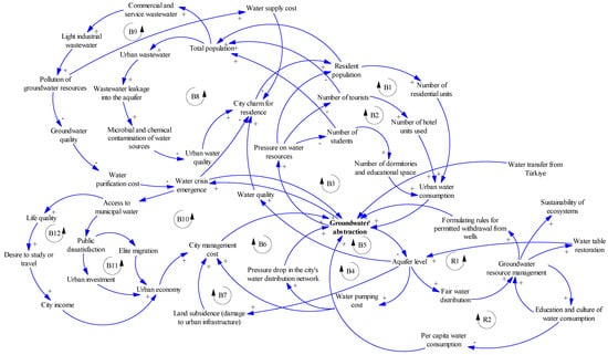
Figure 27.
The group model obtained from the workshop for groundwater management in the urban sector.
As can be seen from Figure 27, this model has two reinforcing feedback loops and twelve balancing feedback loops. In balancing feedback loops 1, 2, and 3, the urban resident population, the number of tourists, and the number of students affect the number of residential units, the number of hotel units used, and the number of dormitories and training spaces used, respectively (similarly). These units, in turn, affect urban water consumption (similarly). Urban water consumption affects groundwater abstraction (similarly) [51], and groundwater abstraction also leads to pressure on water resources (similarly). Finally, pressure on water resources has an adverse effect on the urban resident population, the number of tourists, and the number of students [51] (oppositely).
Balancing feedback loops 4 to 7 address the impacts of groundwater abstraction on various issues. Groundwater abstraction affects the aquifer level (oppositely). The aquifer level affects the water pumping cost (similarly); the water pumping cost affects the pressure drop in the city’s water distribution network (similarly) [52]; and then the pressure drop in the city’s water distribution network affects groundwater abstraction (similarly) (balancing feedback loop 4). On the other hand, the aquifer level affects water quality (similarly); water quality affects the city’s attractiveness for residence (similarly); the city’s attractiveness affects the resident population (similarly); and, finally, the resident population affects groundwater abstraction (similarly) (balancing feedback loop 5). On the other hand, the aquifer level, which similarly affects the cost of pumping water, also affects the cost of city management (similarly), which in turn affects groundwater abstraction (similarly), because, as the cost of city management increases [53], groundwater abstraction is used as a temporary solution to meet the city’s water demand [54] (balancing feedback loop 6). On the other hand, the aquifer level also affects land subsidence (damage to urban infrastructure) (similarly), which also affects the cost of city management (similarly) and ultimately affects groundwater abstraction (similarly) (balancing feedback loop 7).
In balancing feedback loop 8, the total population affects urban wastewater (similarly); urban wastewater affects wastewater leakage into the aquifer (similarly); wastewater leakage into the aquifer affects the microbial and chemical contamination of water sources (similarly) [55]; this pollution of water sources affects the water quality (oppositely); the water quality affects the city’s attractiveness for residence (similarly) [56]; and, finally, the city’s attractiveness affects the total population (similarly). On the other hand, in balancing feedback loop 9, the total population affects commercial and service wastewater (similarly); commercial and service wastewater affects light industrial wastewater, including wastewater from restaurants, hotels, and grocery stores (similarly); light industrial wastewater affects the pollution of groundwater resources (similarly); the pollution of groundwater resources affects groundwater quality (oppositely); groundwater quality affects the water purification cost (oppositely); the water purification cost affects water crisis emergence (oppositely) [57] (because when more money is spent on water treatment, water crisis emergence can be reduced and vice versa); water crisis emergence affects the city’s attractiveness for residence (oppositely); and, finally, the city’s attractiveness for residence affects the total population of the city (similarly).
In balancing feedback loops 10 to 12, groundwater abstraction affects water crisis emergence (similarly), and water crisis emergence affects access to municipal water (oppositely). Access to municipal water affects public dissatisfaction (oppositely) [58]. Public dissatisfaction affects elite migration (similarly); elite migration affects the city’s economy (oppositely); the city’s economy affects the city management cost (similarly); and, finally, the city management cost affects groundwater abstraction (similarly) (balancing feedback loop 10). Meanwhile, public dissatisfaction also affects urban investment (oppositely) [59], and urban investment affects the city’s economy (similarly); furthermore, the city’s economy affects the city management cost and groundwater abstraction (balancing feedback loop 11). On the other hand, access to urban water affects quality of life (similarly); quality of life affects the desire of individuals to study in or travel to the given area (similarly); the desire to study or travel affects urban income (similarly); urban income also affects the city’s economy (similarly); and, subsequently, the city’s economy affects the cost of city management and water withdrawal from groundwater resources (balancing feedback loop 12).
There are also two reinforcing feedback loops in Figure 27. The rules for withdrawal from wells affect groundwater abstraction (oppositely) [60]; groundwater abstraction affects the aquifer level (inversely); the aquifer level affects fair water distribution (similarly); fair water distribution affects groundwater management (similarly); and, finally, groundwater management affects the rules for withdrawal from wells (similarly) (reinforcing feedback loop 1). On the other hand, groundwater abstraction affects the aquifer level, fair water distribution, and groundwater resource management; meanwhile, groundwater resource management, education, and the culture of water consumption influence each other reciprocally (similarly) [61]; education and the culture of water consumption influence the per capita water consumption (oppositely); and, finally, the per capita water consumption affects groundwater abstraction (similarly) (reinforcing feedback loop 2).
5.2. Agricultural Sector
A preliminary cause-and-effect model of groundwater management in the Güzelyurt region, considering intensive and water-intensive agriculture, was prepared based on the structured and semi-structured interviews and the results obtained from them, with a greater emphasis on the population growth of the region and its water needs, water-intensive agriculture and the pressure on water resources, the pollution of groundwater resources due to agriculture, groundwater resource management, water management policies and productivity, and the negative effects of mismanagement on groundwater resources. This model is shown in Figure 28.
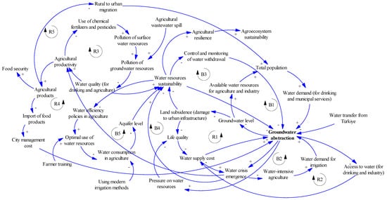
Figure 28.
The preliminary model of groundwater management in the agricultural sector.
As can be seen from Figure 28, this model has five reinforcing feedback loops and five balancing feedback loops. In balancing feedback loop 1, the total population affects the water demand (for drinking and municipal services) (similarly); the water demand affects groundwater abstraction (similarly); groundwater abstraction affects groundwater levels (oppositely); groundwater levels affect the water resources available for agriculture and industry (similarly); and the water resources available for agriculture and industry affect the total population (similarly) (because, as the water resources available for agriculture and industry decrease, fewer people are attracted to the area to live and work, and vice versa).
In balancing feedback loop 2, water-intensive agriculture affects the water demand for irrigation (similarly); the water demand for irrigation affects groundwater abstraction (similarly); groundwater abstraction affects the groundwater level (oppositely); the groundwater level affects land subsidence (damage to urban infrastructure) (oppositely); land subsidence affects quality of life (oppositely); quality of life affects the water supply cost (oppositely); the water supply cost affects water crisis emergence (similarly); and, finally, water crisis emergence affects water-intensive agriculture (oppositely). In the meantime, the water supply cost affects groundwater abstraction (similarly), which forms reinforcing feedback loop 1, with relationships between the groundwater levels, land subsidence, quality of life, and ultimately the water supply cost. Moreover, by considering again the water supply cost affecting groundwater abstraction (similarly), the impact of groundwater abstraction on water availability (for drinking and industry) (oppositely), and the impact of water availability on the water supply cost (oppositely), reinforcing feedback loop 2 is formed.
In reinforcing feedback loop 3, the use of chemical fertilizers and pesticides affects the pollution of surface water resources (similarly); the pollution of surface water resources affects the pollution of groundwater resources (similarly); the pollution of groundwater resources affects the quality of water for drinking and agriculture (oppositely); the quality of water affects agricultural productivity (similarly); and agricultural productivity affects the use of chemical fertilizers and pesticides (oppositely) (because the lower the agricultural productivity, the more farmers resort to the use of chemical fertilizers and pesticides to improve the situation, and vice versa).
In balancing feedback loop 3, the control and monitoring of water withdrawal affects groundwater abstraction (oppositely); groundwater abstraction affects the aquifer level (oppositely); the aquifer level affects land subsidence (oppositely); land subsidence affects water resource sustainability (oppositely); and water resource sustainability affects the control and monitoring of water withdrawal (oppositely). On the other hand, considering the relationship between the control and monitoring of water withdrawal and groundwater abstraction, groundwater abstraction affects the pressure on water resources (similarly); the pressure on water resources affects quality of life (oppositely); quality of life affects water crisis emergence in agricultural areas (oppositely); and water crisis emergence affects water resource sustainability (oppositely). Thus, the relationship between water resource sustainability and the control and monitoring of water withdrawal is established as before, forming balancing feedback loop 4.
In balancing feedback loop 5, water efficiency policies in agriculture affect the optimal use of water resources (similarly); the optimal use of water resources affects water consumption in agriculture (oppositely); water consumption in agriculture affects the aquifer level (oppositely); the aquifer level affects water resource sustainability (similarly); and, finally, water resource sustainability affects water efficiency policies (oppositely) (because, with water resource sustainability, the implementation of water efficiency policies decreases, and vice versa). Moreover, in this loop, there are cases outside the feedback loop, such as the opposite effects of using modern irrigation methods on water consumption in agriculture, as well as educating farmers about the better use of water resources, which similarly affect the optimal use of water resources.
In reinforcing feedback loop 4, groundwater abstraction affects water crisis emergence (similarly); water crisis emergence affects agricultural productivity (oppositely); agricultural productivity affects agricultural production (similarly); agricultural production affects the import of food products (oppositely); the import of food products affects the city management cost (similarly); and, finally, the city management cost affects groundwater abstraction (similarly) (because, as the city management cost increases, the tendency towards using simpler solutions, such as increased abstraction from groundwater resources, increases, and vice versa). Moreover, considering the relationships between groundwater abstraction, water crisis emergence, agricultural productivity, and agricultural production, the opposite effects of agricultural production on rural-to-urban migration and the effects of this migration similarly on groundwater abstraction form reinforcing feedback loop 5.
Following the above description of the loops in the preliminary model for the agricultural sector, the main group model that emerged from the workshop discussion is presented below. The group model developed is based on population growth and water needs, water-intensive agriculture and water resource consumption, groundwater pollution, feedback in cases of improper groundwater resource management, water efficiency policies in agriculture, the long-term effects of groundwater over-abstraction, and water and economic crises resulting from these issues. This model is shown in Figure 29.
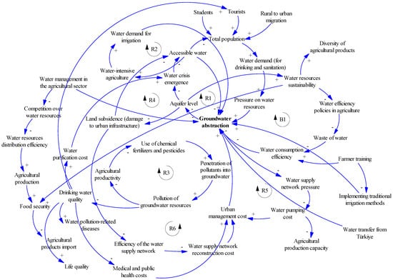
Figure 29.
The group model obtained from the workshop for groundwater management in the agricultural sector.
As can be seen from Figure 29, this model has six reinforcing feedback loops and one balancing feedback loop.
In reinforcing feedback loop 1, the total population affects the water demand (for drinking and sanitation) (similarly); the water demand affects pressure on water resources (similarly); pressure on water resources affects groundwater abstraction (similarly); groundwater abstraction affects aquifer levels (similarly); aquifer levels affect water crisis emergence (oppositely); water crisis emergence affects the accessible water (for agriculture) (oppositely) [57]; and, finally, the accessible water affects the total population (oppositely) (because, as the accessible water decreases, fewer people are attracted to the area in question and vice versa). In reinforcing feedback loop 2, water-intensive agriculture affects the water demand for irrigation (similarly) [62]; the water demand for irrigation affects groundwater abstraction (similarly); groundwater abstraction affects the aquifer level (oppositely); the aquifer level affects water crisis emergence (oppositely); water crisis emergence affects the accessible water (oppositely); and, finally, the accessible water affects water-intensive agriculture (similarly) (because, as the accessible water increases, the amount of water-intensive agriculture usually increases, because it is believed that there is plenty of water available and water-intensive agriculture is not a problem, and vice versa).
In reinforcing feedback loop 3, the use of chemical fertilizers and pesticides affects the penetration of pollutants into groundwater (similarly); the penetration of pollutants into groundwater affects the pollution of groundwater resources (microbial and chemical) (similarly); the pollution of groundwater resources affects agricultural productivity (oppositely) [63]; and, finally, agricultural productivity affects the use of chemical fertilizers and pesticides (oppositely) (because the lower the agricultural productivity, the greater the motivation to use chemical fertilizers and pesticides and vice versa). In reinforcing feedback loop 4, groundwater abstraction affects the aquifer level (oppositely); the aquifer level affects land subsidence (damage to urban and agricultural infrastructure) (oppositely) [64]; land subsidence affects water availability (oppositely); and, finally, water availability affects groundwater abstraction (oppositely). Among reinforcing feedback loops 3 and 4, the cause-and-effect relationships between groundwater pollution, drinking water quality, water treatment costs, water crisis emergence, and groundwater abstraction should be considered, as they link these two feedback loops together. Moreover, in reinforcing feedback loop 4, water management in the agricultural sector affects groundwater abstraction as well as competition over water resources (between agriculture, drinking water, and industry) [65], the water resource distribution efficiency, and consequently agricultural production and ultimately food security, which is related to the import of agricultural products [66].
In reinforcing feedback loop 5, groundwater abstraction affects the water supply network pressure (oppositely); the water supply network pressure affects the water pumping cost (oppositely); the water pumping cost affects the urban management cost (similarly); and, finally, the urban management cost affects groundwater abstraction (similarly) (because, as the urban management cost increases, the use of measures like groundwater abstraction, which are usually less expensive, increases, and vice versa). In reinforcing feedback loop 6, groundwater abstraction affects the aquifer level (oppositely); the aquifer level affects land subsidence (damage to urban infrastructure) (oppositely); land subsidence and damage to urban infrastructure affect the efficiency of the water supply network (oppositely) [67]; the efficiency of the water supply network affects the water supply network’s reconstruction cost (oppositely); the water supply network’s reconstruction cost affects the urban management cost (similarly); and, finally, the urban management cost affects groundwater abstraction (similarly).
In balancing feedback loop 1, water efficiency policies in agriculture affect the waste of water (oppositely); the waste of water affects the water consumption efficiency (oppositely) [68]; the water consumption efficiency affects groundwater abstraction (oppositely); groundwater abstraction affects the aquifer level (oppositely); the aquifer level affects water resource sustainability (similarly); and, finally, water resource sustainability affects water efficiency policies in agriculture (oppositely) (because, with increasing water resource sustainability, there is a reduced need for water efficiency policies in agriculture and vice versa) [69].
5.3. Model Validation Through Stock–Flow Diagram Model
We next examine how the strategies introduced in the previous sections will affect the quantity and quality of groundwater in the study area in the future. For this purpose, the groundwater level was modeled to assess the quantity, and the electrical conductivity was modeled to assess the quality, for station A. This modeling was performed for three periods: the short term (25 years), medium term (50 years), and long term (75 years). Therefore, predictions were made for 2025 to 2100, and these are presented along with feasible scenarios. In Figure 30, the SFD for this research is presented.
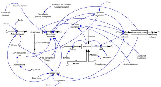
Figure 30.
SFD for Güzelyurt’s groundwater situation.
While the SFD for Güzelyurt’s groundwater situation is shown in Figure 30, in order to model and predict the future situation and better manage the quantity and quality of groundwater, possible scenarios using the strategies introduced in the previous sections were also applied in the modeling. A total of three scenarios were introduced and applied. A fourth scenario (scenario 4) is also possible, which is the sum of all scenarios simultaneously. However, this cannot have a cumulative effect—under some strategies, and by its nature, the scenarios overlap. The scenarios are as follows.
Scenario 1: “Cross-Border and Strategic Water Supply Management” related to “water release from the Southern Cyprus side” and “managed use of water transferred from Turkey to Northern Cyprus” strategies. Scenario 2: “Local Efficiency, Demand Reduction, and Groundwater Protection” related to “controlling the population of the region”, “smart and sustainable urban management”, “water-intensive agricultural management”, “optimal use of water resources”, “modern irrigation technologies”, and “water withdrawal control” strategies. Scenario 3: “Cultural Shift and Public Engagement” related to “education and culture of people” strategy. Each scenario uses a different strategy—external coordination, internal efficiency, and cultural transformation—all crucial for a holistic groundwater management plan in Northern Cyprus. In each of the scenarios, for implementation in the model, the relevant variables were increased to the maximum level that could be implemented. In Figure 31 and Figure 32, the SFD modeling results for the groundwater level and electrical conductivity are presented.
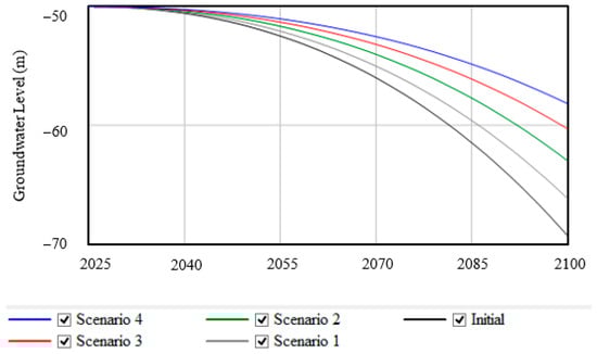
Figure 31.
SFD modeling results for groundwater level for station A.
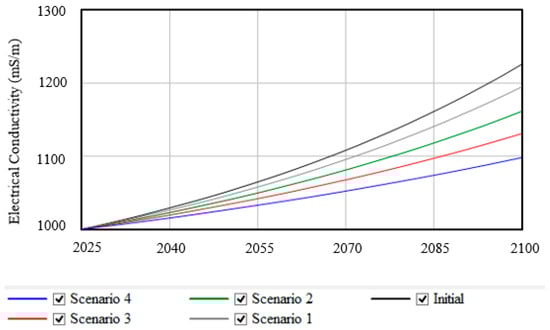
Figure 32.
SFD modeling results for electrical conductivity for station A.
As seen in Figure 31, the groundwater level will continue to decrease in the future for station A. This decrease for station A, which has increased in recent years due to issues such as water transfer from Turkey to the region, will also continue in the future and in the long term because, as mentioned earlier, inter-basin water transfers cannot be a sustainable long-term strategy. Although this decrease is very small at first, in the long term, this station will also experience a decrease in groundwater levels from about −50 m to −70 m. Upon adopting scenarios 1 to 3, this situation will improve; finally, by adopting scenario 4, which is the sum of all previous scenarios, the groundwater level can be decreased by only about 8 m to −58 m.
In Figure 32, it can be seen that an increase in electrical conductivity in the future can be predicted for station A and the study area. For station A, the electrical conductivity value will increase from 1000 s/m in 2025 to 1220 s/m in 2100, which can be improved by adopting different scenarios (scenarios 1 to 3). In the best case, when all strategies are combined and scenario 4 is implemented, the electrical conductivity value at station A could reach 1100 s/m, which is a more than 50% improvement.
5.4. Strategies and Iceberg Model
From Figure 26, Figure 27, Figure 28 and Figure 29, which have been validated and controlled using various scientific sources, it can be seen that there are different reinforcing and balancing loops in both the urban and agricultural sectors. These feedback loops, and the different cause-and-effect relationships existing in the current situation in the study area, have caused the existence of different system archetypes in these structures. In Figure 27 and Figure 29, the balancing loops are subject to balance and “limits to growth” due to the reinforcing loops. Moreover, the transfer of water from Turkey, some of which is used for drinking in Northern Cyprus, while the rest is used in agriculture in the Güzelyurt region, should not serve as a “fix that backfires”. In this case, the root cause of the groundwater management problem in the region will not be resolved, and we will also see side effects of temporary solutions, such as migration from neighboring areas to the Güzelyurt region, which will increase the pressure on its water resources. Moreover, in the region, due to the presence of citizens, agriculture, tourism, and students, the system archetype of “success for the successful” is also very likely, because each of these successful sectors can obtain greater funding from the government and will increase the pressure on the groundwater resources due to their increasing populations. There is also a “tragedy of the commons” among farmers, which can be prevented to some extent by establishing laws and policies on groundwater exploitation and water efficiency policies in agriculture.
The strategies and solutions implemented, and the changes necessary to better manage the groundwater resources in the study area, are presented in this section using the iceberg model. The iceberg model is shown in Figure 33.
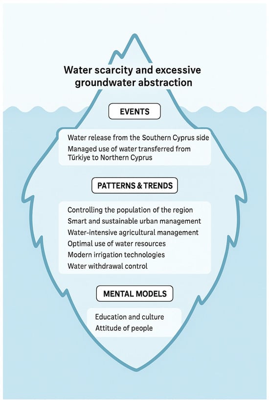
Figure 33.
Iceberg model for water scarcity and excessive groundwater abstraction.
In this case, the “event” or problem is the water scarcity and excessive groundwater abstraction in the study area. Solutions that can be introduced in the “pattern” section, which are mid-range leverage points [70] and are considered minor and partial solutions, include measures such as water release from the Southern Cyprus side in the basin in question and the managed use of water transferred from Turkey to Northern Cyprus. Solutions that can be introduced in the “structure of the system” section, which are deeper-level points [70] and are considered fundamental solutions, include the desirable reinforcing and balancing feedback loops shown in Figure 26 and Figure 28, such as controlling the population of the region (including tourists, migrants, and students), smart and sustainable urban management that improves quality of life and facilitates and ensures the attraction of new, beneficial investments, water-intensive agricultural management, the optimal use of water resources, modern irrigation technologies, and water withdrawal control. A basic solution that can be introduced at the “mental model” level [70] is the education and culture of the population. This includes residents, politicians, farmers, and all other stakeholders. Although this [71] is more difficult to change compared to the other aspects, its results are clearly more significant compared to any other strategy [70]. It is by educating the people of the city that water waste will be reduced; it is by educating farmers that modern agronomy and irrigation can be achieved; and it is by educating politicians that the optimal water efficiency policies will be implemented in all sectors, especially in the agricultural sector.
6. Conclusions
This study highlights the critical complexity of groundwater resource management in the Güzelyurt region of Northern Cyprus through a systems thinking approach, employing SD and GMB techniques. The identification of multiple reinforcing and balancing feedback loops in both the urban and agricultural sectors reveals the intricate interplay between population dynamics, water consumption, groundwater abstraction, and environmental impacts such as land subsidence and water quality degradation. The models developed underscore how short-term fixes, such as external water transfers, may temporarily alleviate the scarcity but risk exacerbating underlying systemic issues if not coupled with sustainable policies. These findings emphasize the necessity of adopting a holistic perspective that recognizes the interconnectedness of the social, economic, and environmental factors affecting water resource sustainability.
Moving forward, the application of the iceberg model in this study provides a valuable framework for the prioritization of intervention strategies across different system layers—from visible events to deeper mental models. Fundamental solutions such as regulated groundwater withdrawal, smart urban and agricultural water management, and the adoption of modern irrigation technologies address systemic structures, while the pivotal roles of education and cultural change emerge as leverage points with the greatest long-term impacts. Engaging all stakeholders in fostering awareness and responsible water use behaviors is essential in ensuring resilient and equitable groundwater management. Ultimately, this research demonstrates that integrating stakeholder-driven system dynamics modeling with targeted, multi-level strategies offers a promising pathway to mitigating water scarcity challenges and securing sustainable water resources for the region’s future.
The GMB-SD approach offers distinct strengths over conventional hydrologic models by integrating stakeholder knowledge, system feedback, and socio-institutional factors into water management. Unlike traditional models that focus primarily on quantitative, physical processes such as flow rates and recharge–discharge dynamics, GMB-SD emphasizes the co-creation of qualitative and quantitative models to capture human–environment interactions, policy dynamics, and behavioral responses. This participatory modeling process fosters a shared understanding, trust, and adaptive capacity among stakeholders. However, implementation faces challenges such as stakeholder resistance, limited data for calibration, time-intensive facilitation, and the complexity of translating qualitative insights into rigorous simulations. To address these, adaptive management options include iterative model refinement, scenario planning, stakeholder training, and integrating GMB-SD with conventional models to support both technical accuracy and institutional learning in dynamic water systems.
Author Contributions
Conceptualization, F.B., V.N. and H.G.; methodology, F.B.; software, F.B.; data curation, Y.K.; writing—original draft preparation, F.B.; supervision, V.N. and H.G. All authors have read and agreed to the published version of the manuscript.
Funding
This research received no external funding.
Data Availability Statement
No new data were created.
Conflicts of Interest
The authors declare no conflicts of interest.
Abbreviations
The following abbreviations are used in this manuscript:
| SD | System dynamics |
| QSDA | Qualitative system dynamics approach |
| GMB | Group model building |
| CLD | Causal loop diagram |
References
- Van Vliet, M.T.; Jones, E.R.; Flörke, M.; Franssen, W.H.; Hanasaki, N.; Wada, Y.; Yearsley, J.R. Global water scarcity including surface water quality and expansions of clean water technologies. Environ. Res. Lett. 2021, 16, 024020. [Google Scholar] [CrossRef]
- Kassem, Y.; Gökçekuş, H.; Mosbah, A.A.S. Prediction of monthly precipitation using various artificial models and comparison with mathematical models. Environ. Sci. Pollut. Res. 2023, 30, 41209–41235. [Google Scholar] [CrossRef]
- Gökçekuş, H.; Bolouri, F. Transboundary Waters and Their Status in Today’s Water-Scarce World. Sustainability 2023, 15, 4234. [Google Scholar] [CrossRef]
- Łukasik, M.; Dąbrowska, D. Groundwater quality testing in the area of municipal waste landfill sites in Dąbrowa Górnicza (southern Poland). Environ. Socio-Econ. Stud. 2022, 10, 13–21. [Google Scholar] [CrossRef]
- Dąbrowska, D.; Sołtysiak, M.; Biniecka, P.; Michalska, J.; Wasilkowski, D.; Nowak, A.; Nourani, V. Application of hydrogeological and biological research for the lysimeter experiment performance under simulated municipal landfill condition. J. Mater. Cycles Waste Manag. 2019, 21, 1477–1487. [Google Scholar] [CrossRef]
- Baghanam, A.H.; Vakili, A.T.; Nourani, V.; Dąbrowska, D.; Soltysiak, M. AI-based ensemble modeling of landfill leakage employing a lysimeter, climatic data and transfer learning. J. Hydrol. 2022, 612, 128243. [Google Scholar] [CrossRef]
- Bolouri, F.; Gökçekuş, H.; Nourani, V. Management of Emerging Pollutants with a Circular Economy Approach: Lessons from Developed Countries and a Case Study in Northern Cyprus. In Emerging Pollutants. Advances in Water Security; Zandaryaa, S., Fares, A., Eckstein, G., Eds.; Springer: Cham, Switzerland, 2025; pp. 317–332. [Google Scholar]
- Ohenhen, L.O.; Zhai, G.; Lucy, J.; Werth, S.; Carlson, G.; Khorrami, M.; Onyike, F.; Sadhasivam, N.; Tiwari, A.; Ghobadi-Far, K.; et al. Land subsidence risk to infrastructure in US metropolises. Nat. Cities 2025, 2, 543–554. [Google Scholar] [CrossRef]
- Ghasemi, A.; Saghafian, B.; Golian, S. System dynamics approach for simulating water resources of an urban water system with emphasis on sustainability of groundwater. Environ. Earth Sci. 2017, 76, 1–15. [Google Scholar] [CrossRef]
- Chen, X.; Xu, Q.; Cai, J. Research on the urban water resources carrying capacity by using system dynamics simulation. Hydrol. Res. 2023, 54, 418–434. [Google Scholar] [CrossRef]
- Zarghami, M.; Akbariyeh, S. System dynamics modeling for complex urban water systems: Application to the city of Tabriz, IranResour. Conserv. Recycl. 2012, 60, 99–106. [Google Scholar] [CrossRef]
- Wei, T.; Lou, I.; Yang, Z.; Li, Y. A system dynamics urban water management model for Macau, China. J. Environ. Sci. 2016, 50, 117–126. [Google Scholar] [CrossRef] [PubMed]
- Hovmand, P.S. Group Model Building and Community-Based System Dynamics Process; Springer: New York, NY, USA, 2014; pp. 17–30. [Google Scholar]
- Vennix, J.A.; Akkermans, H.A.; Rouwette, E.A. Group model-building to facilitate organizational change: An exploratory study. Syst. Dyn. Rev. 1996, 12, 39–58. [Google Scholar] [CrossRef]
- Richmond, B. Systems thinking: Critical thinking skills for the 1990s and beyond. Syst. Dyn. Rev. 1993, 9, 113–133. [Google Scholar] [CrossRef]
- Forrester, J.W. Industrial dynamics. J. Oper. Res. Soc. 1997, 48, 1037–1041. [Google Scholar] [CrossRef]
- Sterman, J. System Dynamics: Systems Thinking and Modeling for a Complex World; Massachusetts Institute of Technology. Engineering Systems Division, UAS: Cambridge, MA, USA, 2002; pp. 1–29. [Google Scholar]
- Richardson, G.P. Problems in causal loop diagrams revisited. Syst. Dyn. Rev. 1997, 13, 247–252. [Google Scholar] [CrossRef]
- Wolstenholme, E. Using generic system archetypes to support thinking and modelling. Syst. Dyn. Rev. 2004, 20, 341–356. [Google Scholar] [CrossRef]
- Mirchi, A.; Madani, K.; Watkins, D.; Ahmad, S. Synthesis of system dynamics tools for holistic conceptualization of water resources problems. Water Resour. Manag. 2012, 26, 2421–2442. [Google Scholar] [CrossRef]
- Madani, K.; Mariño, M.A. System dynamics analysis for managing Iran’s Zayandeh-Rud river basin. Water Resour. Manag. 2009, 23, 2163–2187. [Google Scholar] [CrossRef]
- Bagheri, A.; Hjorth, P. A framework for process indicators to monitor for sustainable development: Practice to an urban water system. Environ. Dev. Sustain. 2007, 9, 143–161. [Google Scholar] [CrossRef]
- Hardin, G. The tragedy of the commons: The population problem has no technical solution; it requires a fundamental extension in morality. Science 1968, 162, 1243–1248. [Google Scholar] [CrossRef]
- Loáiciga, H.A. Analytic game—Theoretic approach to ground-water extraction. J. Hydrol. 2004, 297, 22–33. [Google Scholar] [CrossRef]
- Madani, K. Game theory and water resources. J. Hydrol. 2010, 381, 225–238. [Google Scholar] [CrossRef]
- Ergil, M.E. The salination problem of the Guzelyurt aquifer, Cyprus. Water Res. 2000, 34, 1201–1214. [Google Scholar] [CrossRef]
- Arslan, B.; Akün, E. Management, contamination and quality evaluation of groundwater in North Cyprus. Agric. Water Manag. 2019, 222, 1–11. [Google Scholar] [CrossRef]
- Türker, U.; Hansen, B.R. River Basin Management and Characterization of Water Bodies in North Cyprus. In Proceedings of the 10th International Congress on Advances in Civil Engineering, Ankara, Turkey, 17–19 October 2012; pp. 17–19. [Google Scholar]
- Gökcekuş, H.; Iravanian, A.; Türker, U.; Oğuz, G.; Sözen, S.; Orhon, D. Massive freshwater transport: A new dimension for integrated water-wastewater management in North Cyprus. Desalin. Water Treat. 2018, 132, 215–225. [Google Scholar] [CrossRef]
- Kassem, Y.; Gökçekuş, H.; Rizza, T. Groundwater Quality Assessment Based on Water Quality Index in Northern Cyprus. Eng. Technol. Appl. Sci. Res. 2022, 12, 8435–8443. [Google Scholar] [CrossRef]
- İpek, C.; Türker, U. Geospatial based groundwater resources susceptibility and contamination risk mapping for Yeşilköy aquifer, Cyprus. Environ. Earth Sci. 2024, 83, 446. [Google Scholar] [CrossRef]
- Richardson, G.P.; Andersen, D.F. Teamwork in group model building. Syst. Dyn. Rev. 1995, 11, 113–137. [Google Scholar] [CrossRef]
- Richmond, B. The strategic forum: Aligning objectives, strategy and process. Syst. Dyn. Rev. 1997, 13, 131–148. [Google Scholar] [CrossRef]
- Lane, D.C. Diagramming conventions in system dynamics. J. Oper. Res. Soc. 2000, 51, 241–245. [Google Scholar] [CrossRef]
- Andersen, D.F.; Vennix, J.A.; Richardson, G.P.; Rouwette, E.A. Group model building: Problem structuring, policy simulation and decision support. J. Oper. Res. Soc. 2007, 58, 691–694. [Google Scholar] [CrossRef]
- Richardson, G.P. Concept models in group model building. Syst. Dyn. Rev. 2013, 29, 42–55. [Google Scholar] [CrossRef]
- Andersen, D.F.; Richardson, G.P. Scripts for group model building. Syst. Dyn. Rev. 1997, 13, 107–129. [Google Scholar] [CrossRef]
- Luna-Reyes, L.F.; Martinez-Moyano, I.J.; Pardo, T.A.; Cresswell, A.M.; Andersen, D.F.; Richardson, G.P. Anatomy of a group model-building intervention: Building dynamic theory from case study research. Syst. Dyn. Rev. 2006, 22, 291–320. [Google Scholar] [CrossRef]
- Ackermann, F.; Andersen, D.F.; Eden, C.; Richardson, G.P. ScriptsMap: A tool for designing multi-method policy-making workshops. Omega 2011, 39, 427–434. [Google Scholar] [CrossRef]
- Hovmand, P.S.; Andersen, D.F.; Rouwette, E.; Richardson, G.P.; Rux, K.; Calhoun, A. Group model-building ‘scripts’ as a collaborative planning tool. Syst. Res. Behav. Sci. 2012, 29, 179–193. [Google Scholar] [CrossRef]
- Voinov, A.A. Participatory modeling for sustainability. In Encyclopedia of Sustainable Technologies; Elsevier: London, UK, 2017; pp. 33–39. [Google Scholar]
- Vennix, J.A.M. Group Model Building: Facilitating Team Learning Using System Dynamics; John Wiley & Sons Ltd.: Hoboken, NJ, USA, 1996. [Google Scholar]
- Sterman, J.D. All Models Are Wrong: Reflections on Becoming a Systems Scientist. Syst. Dyn. Rev. 2002, 18, 501–531. [Google Scholar] [CrossRef]
- Reed, M.S.; Graves, A.; Dandy, N.; Posthumus, H.; Hubacek, K.; Morris, J.; Prell, C.; Quinn, C.H.; Stringer, L.C. Who’s in and Why? A Typology of Stakeholder Analysis Methods for Natural Resource Management. J. Environ. Manag. 2009, 90, 1933–1949. [Google Scholar] [CrossRef]
- Al-samarraie, H.; Hurmuzan, S. A Review of Brainstorming Techniques in Higher Education. Think. Ski. Creat. 2017, 27, 78–91. [Google Scholar] [CrossRef]
- Pattison, P.E.; Robins, G.L.; Snijders, T.A.B.; Wang, P. Conditional Estimation of Exponential Random Graph Models from Snowball Sampling Designs. J. Math. Psychol. 2013, 57, 284–296. [Google Scholar] [CrossRef]
- Sterman, J.D. Bussiness Dynamics. Systems Thinking and Modeling for a Complex World; Shelstad, J.J., Ed.; McGraw-Hill Higher Education: New York, NY, USA, 2000. [Google Scholar]
- Hassanzadeh, E.; Elshorbagy, A.; Wheater, H.; Gober, P. Managing Water in Complex Systems: An Integrated Water Resources Model for Saskatchewan, Canada. Environ. Model. Softw. 2014, 58, 12–26. [Google Scholar] [CrossRef]
- Monat, J.P.; Gannon, T.F. What is systems thinking? A review of selected literature plus recommendations. Am. J. Syst. Sci. 2015, 4, 11–26. [Google Scholar]
- Lee, H.; Lee, H. Analysis and effects of high school students’ systems thinking using iceberg (IB) model. J. Korean Assoc. Sci. Educ. 2017, 37, 611–624. [Google Scholar]
- Gejl, R.N.; Rygaard, M.; Henriksen, H.J.; Rasmussen, J.; Bjerg, P.L. Understanding the impacts of groundwater abstraction through long-term trends in water quality. Water Res. 2019, 156, 241–251. [Google Scholar] [CrossRef] [PubMed]
- Taftazani, R.; Kazama, S.; Takizawa, S. Spatial analysis of groundwater abstraction and land subsidence for planning the piped water supply in Jakarta, Indonesia. Water 2022, 14, 3197. [Google Scholar] [CrossRef]
- Foster, S.S. The interdependence of groundwater and urbanisation in rapidly developing cities. Urban Water 2001, 3, 185–192. [Google Scholar] [CrossRef]
- De Graaf, I.E.M.; Van Beek, L.P.H.; Wada, Y.; Bierkens, M.F.P. Dynamic attribution of global water demand to surface water and groundwater resources: Effects of abstractions and return flows on river discharges. Adv. Water Resour. 2014, 64, 21–33. [Google Scholar] [CrossRef]
- Dizer, H.; Hagendorf, U. Microbial contamination as an indicator of sewer leakage. Water Res. 1991, 25, 791–796. [Google Scholar] [CrossRef]
- Liu, Y.; Zhang, L.; Wang, D.; Shi, Y.; Tong, L.; Chen, F.; Li, X.; Dong, C.; Zhang, J. Characterization of microbial communities in urban subway: Connotation for indoor environment quality and public health. Air Qual. Atmos. Health 2024, 17, 1401–1413. [Google Scholar] [CrossRef]
- Jury, W.A.; Vaux, H.J., Jr. The emerging global water crisis: Managing scarcity and conflict between water users. Adv. Agron. 2007, 95, 1–76. [Google Scholar]
- Curry, L.L. Consumer Attitudes Toward Public Water Supply Quality: Dissatisfaction and Alternative Water Sources; Illinois State Water Survey: Champaign, IL, USA, 1983. [Google Scholar]
- Lyons, W.E.; Lowery, D. Citizen responses to dissatisfaction in urban communities: A partial test of a general model. J. Politics 1989, 51, 841–868. [Google Scholar] [CrossRef]
- Nelson, R.L.; Perrone, D. Local groundwater withdrawal permitting laws in the south-western US: California in comparative context. Groundwater 2016, 54, 747–753. [Google Scholar] [CrossRef]
- Tójar-Hurtado, J.C.; Mena-Rodríguez, E.; Fernández-Jiménez, M.Á. Spanish agriculture and water: Educational implications of water culture and consumption from the farmers’ perspective. Water 2017, 9, 964. [Google Scholar] [CrossRef]
- Li, C.; Jiang, T.T.; Luan, X.B.; Yin, Y.L.; Wu, P.T.; Wang, Y.B.; Sun, S.K. Determinants of agricultural water demand in China. J. Clean. Prod. 2021, 288, 125508. [Google Scholar] [CrossRef]
- Okorogbona, A.O.; Denner, F.D.; Managa, L.R.; Khosa, T.B.; Maduwa, K.; Adebola, P.O.; Amoo, S.O.; Ngobeni, H.M.; Macevele, S. Water quality impacts on agricultural productivity and environment. Sustain. Agric. Rev. 2018, 27, 1–35. [Google Scholar]
- Bagheri-Gavkosh, M.; Hosseini, S.M.; Ataie-Ashtiani, B.; Sohani, Y.; Ebrahimian, H.; Morovat, F.; Ashrafi, S. Land subsidence: A global challenge. Sci. Total Environ. 2021, 778, 146193. [Google Scholar] [CrossRef]
- Siyal, A.W.; Gerbens-Leenes, P.W.; Vaca-Jiménez, S.D. Freshwater competition among agricultural, industrial, and municipal sectors in a water-scarce country. Lessons of Pakistan’s fifty-year development of freshwater consumption for other water-scarce countries. Water Resour. Ind. 2023, 29, 100206. [Google Scholar] [CrossRef]
- Strzepek, K.; Boehlert, B. Competition for water for the food system. Philos. Trans. R. Soc. B 2010, 365, 2927–2940. [Google Scholar] [CrossRef]
- Bucx, T.H.M.; Van Ruiten, C.J.M.; Erkens, G.; De Lange, G. An integrated assessment framework for land subsidence in delta cities. Proc. Int. Assoc. Hydrol. Sci. 2015, 372, 485–491. [Google Scholar] [CrossRef]
- Liu, B.; Li, Y.; Hou, R.; Wang, H. Does urbanization improve industrial water consumption efficiency? Sustainability 2019, 11, 1787. [Google Scholar] [CrossRef]
- Yadav, M.; Vashisht, B.B.; Jalota, S.K.; Jyolsna, T.; Singh, S.P.; Kumar, A.; Kumar, A.; Singh, G. Improving Water efficiencies in rural agriculture for sustainability of water resources: A review. Water Resour. Manag. 2024, 38, 3505–3526. [Google Scholar] [CrossRef]
- Kellner, E. Identifying leverage points for shifting Water-Energy-Food nexus cases towards sustainability through the Networks of Action Situations approach combined with systems thinking. Sustain. Sci. 2023, 18, 135–152. [Google Scholar] [CrossRef]
- Fischer, J.; Riechers, M. A leverage points perspective on sustainability. People Nat. 2019, 1, 115–120. [Google Scholar] [CrossRef]
Disclaimer/Publisher’s Note: The statements, opinions and data contained in all publications are solely those of the individual author(s) and contributor(s) and not of MDPI and/or the editor(s). MDPI and/or the editor(s) disclaim responsibility for any injury to people or property resulting from any ideas, methods, instructions or products referred to in the content. |
© 2025 by the authors. Licensee MDPI, Basel, Switzerland. This article is an open access article distributed under the terms and conditions of the Creative Commons Attribution (CC BY) license (https://creativecommons.org/licenses/by/4.0/).