Abstract
To further comprehend kinetic processes in the unsaturated zone, a series of soil column experiments was conducted to simulate downward and upward water movement under variable saturation conditions. High-accuracy spatial and temporal measurements were carried out using the time domain reflectometry—TDR—and Ground-Penetrating Radar—GPR—geophysical methods. Several custom spatial TDR sensors were constructed and used alongside point-measuring TDR sensors, which served as reference points for the calibration of the custom spatial waveguides. The experimental results validated the ability of the custom-made spatial sensors, and the TDR technique in general, to capture water movement and soil moisture changes with high precision during varying wetting processes and demonstrated the complementarity, the limitations, and the potential of the GPR method under the same conditions. The study proved that the combination of the aforementioned measuring technologies provides a better understanding of the kinetic processes that occur in variably saturated conditions.
1. Introduction
High-resolution monitoring of the unsaturated zone plays a key role in understanding the hydrologic processes that govern the interactions between surface water, pore water, and groundwater in the hydrosphere. Various attempts have been made to better comprehend this zone that mainly comprise enhanced soil moisture measurement techniques and numerical modeling methods (e.g., Refs. [1,2,3,4]), and the study of processes at various scales (e.g., Refs. [5,6]). Soil column laboratory experiments can significantly aid these attempts by simulating and analyzing vadose zone processes under controlled conditions [7,8].
Using artificial soil columns to mimic unsaturated zone processes is a widely used and validated laboratory method. Numerous experiments have been conducted to identify the hydraulic characteristics and infiltration rates of soil materials. An artificial soil column permits the control, monitoring, and estimation of infiltration, typically simulating vertical, one-dimensional flows. This is normally accomplished by placing the soil sample in a firm and impermeable casing [9].
The design and development of a soil column setup depends on the goals of each study and for this reason there is no standardized template for all purposes. Each setup has a great impact on the experimental results that are mainly affected by factors such as the existence or lack of macropores, preferential flow paths, and unnatural soil moisture patterns [9]. Therefore, the design of an artificial soil column should be carefully planned and considered. Numerous soil column designs have been presented in the literature. Their dimensions range from a few cm3 to several m3 and can weigh several tons (e.g., Refs. [10,11]).
According to Ref. [9], the three most common materials for the creation of artificial soil columns are plexiglass [12,13], stainless steel [14,15], and glass [16,17], while PTFE-lined steel [18], PVC [19,20], fiberglass [21], and cement [22] are also frequently used. To select the appropriate soil column material, traits like durability, transparency, availability, and potential chemical interference with solutes need to be taken into account.
Depending on the degree of saturation, soil columns are divided into saturated and unsaturated columns. The soil pores of unsaturated columns are filled with both a liquid (such as water) and air, and they are mainly used to replicate vadose zone processes. In contrast, the pores in saturated columns are fully filled with the water in use and are generally used to simulate aquifer processes. The experiments in this study were conducted under both saturated and unsaturated regimes.
Two of the most common measurement techniques in unsaturated soil columns are time domain reflectometry (TDR) for soil moisture estimation and tensiometers for pore water pressure estimation. The data from these two methods can be used to construct the characteristic curve of the soil being studied. A thorough review of the use of TDR in soil column experiments can be found in Ref. [23].
The investigation of hydrological processes using soil columns dates back to the 18th century [9,24]. The majority of the early works, except for the pioneering study of Ref. [25], were conducted in unsaturated soil columns and mainly focused on estimating infiltration rates and the quantity of percolating water [24,26,27]. Studies on transport kinetics and the permeability of porous materials began to emerge after 1940 [28,29,30], alongside the estimation of retention functions, as presented by Refs. [31,32]. In recent years, numerous soil column experiments have been carried out to measure soil water characteristics and infiltration and evapotranspiration rates (e.g., Refs. [33,34], to study contaminant transport (e.g., Refs. [35,36]) and preferential flow mechanisms [37,38], and to assess flow models [39,40]. For example, Ref. [8] developed a soil column setup to simulate mostly non-isothermal unsaturated zone water flows, using spatial TDR sensors to complement the monitoring of soil moisture variations and infiltration front movement along the column.
Soil column experiments can also be engaged to simulate the movement of substances like solutes, contaminants, pesticides, heavy metals, germs, explosive materials, and nutrients in the ground [9]. Monitoring, measuring, and predicting solute movement in the unsaturated zone are fundamental for viable soil and aquifer handling, and many studies have been conducted in this domain (e.g., Refs. [41,42,43,44,45,46], featuring soil column experiments [41,42,47,48]. Ref. [49] conducted a column experiment to improve the estimation of hydraulic properties and soil water retention characteristics to better model and predict water and solute movement in unsaturated soils. Ref. [50] performed soil column percolation tests to enhance the procedure of predicting chemical leaching from contaminated soils, while Refs. [51,52] ran similar percolation and leaching experiments, respectively, utilizing columns of different dimensions.
Even though soil columns have been used for over three centuries, a standard experimental procedure has yet to be developed, mainly due to unique research needs, making the juxtaposition of the results of different studies a complicated task. Soil scientists and hydrogeologists who want to prevent significant design faults, fine-tune the fabrication of their own artificial columns, and ensure the validity of their results should refer to the work of Ref. [9], who wrote a comprehensive paper on the various types of columns and the best practices followed during the execution of experiments found in the literature. The various designs, materials, and dimensions that have been used for the construction of different soil columns, as well as the advantages and drawbacks of each case and the various kinds of soil column experiments, are also mentioned in detail in this paper.
In this study, a series of laboratory experiments was conducted in an artificial soil column filled with quartz sand. The main objective of these experiments was to simulate various types of water flow in the vadose zone and to develop, implement, and evaluate an integrated system for the continuous, real-time, 3-D monitoring of these flows using TDR and GPR techniques. The system involves the design, construction, and evaluation of custom-made elongated TDR sensors. These sensors are calibrated using reference measurements from commercial factory-calibrated point sensors. A key component of the calibration is the implementation and validation of the numerical one-dimensional model by Ref. [53], which estimates soil moisture profiles along the waveguides of a sensor using TDR waveforms. The validation of the developed system in lab conditions led to its application in an infiltration experiment under field conditions, as presented in Ref. [54].
2. Materials and Methods
2.1. Soil Column
To simulate water flows under controlled conditions and evaluate the capability of the custom spatial TDR probes and the entire developed system with various techniques to monitor these flows, an experimental column setup was designed and constructed.
The column is made of poly(methyl methaxcrylate, PMMA (plexiglass), with an inner diameter of 50 cm, a height of 150 cm, and a wall thickness of 0.5 cm (Figure S1a, Supplementary Materials). PMMA was selected as the material of choice for several reasons. It has a dielectric constant of approximately 3 [55], similar to that of the main mineral components of soil (3–12; [56]). The main technical reasons are its increased strength with greater wall thickness, allowing it to bear the cumulative weight of sand and water, especially under saturated conditions, and its transparency, which facilitates the qualitative monitoring of water presence near the column walls and the water level. In general, plexiglass is less prone to scratching and easier to cut and shape compared to other transparent materials, such as glass.
For the purpose of this experiment, the column was filled with quartz sand with a grain size of 0.1 to 0.4 mm and a porosity of 31 to 34%, up to a level of one meter (Figure S1b, Supplementary Materials). The entire setup was positioned on a custom metal base (Figure S1a,c, Supplementary Materials), allowing the sand to be drained through a valve attached at the bottom of the column after each experiment (Figure S1d, Supplementary Materials). A sieve was attached at the drainage outlet at the inner bottom of the column, with a mesh size smaller than the sand grain size to prevent sand passage (Figure S1c, Supplementary Materials).
Several irrigation hoses and nozzles were used as water inlet components, which, depending on the experiment, were placed at different levels and shapes. In this way, water could be inserted from the column surface through rainfall simulation, or from within the sand at different depths.
2.2. TDR Probes and Sensors
In these experiments, two types of TDR sensors were used, commercial sensors for point measurements at specific level intervals, and custom elongated sensors for estimating soil moisture profiles along the length of the sensor as developed and described in Ref. [6].
2.2.1. Point Sensors
The commercial point sensors were used to calibrate and better interpret the measurements of the custom elongated sensors. In this study, five calibrated CS645 3-waveguide point sensors from Campbell Scientific Inc. (Manufacturer: Campbell Scientific Ltd., Loughborough, UK) were used, with a length of 7.5 cm, a waveguide diameter of 0.159 cm and an integrated transformer (balun) to compensate for the impedance differences between the sensors’ waveguides and the coaxial cable (Figure 1). These 5 sensors, henceforth referred to as TDR1, TDR2, TDR3, TDR4, and TDR5, were installed horizontally on the column, at heights of 10 cm, 30 cm, 50 cm, 70 cm, and 90 cm, respectively (Figure 1).

Figure 1.
The five calibrated point sensors (TDR1, TDR2, TDR3, TDR4, and TDR5) are horizontally installed on the column at heights of 10 cm, 30 cm, 50 cm, 70 cm, and 90 cm, respectively, while two custom spatial probes (STDR1 and STDR2), each with a length of 1.5 m, are positioned vertically inside the column.
2.2.2. Custom Elongated Probes
One of the main objectives of this study was to apply custom spatial probes that could be used to accurately measure soil moisture profiles in the deeper parts of the vadose zone. When designing a TDR sensor, the main goal is to achieve a relatively uniform energy distribution in the soil sampling volume. Commercial TDR sensors typically consist of two or three parallel metallic rods that act as waveguides [57,58]. In this study, only 3-waveguide probes were constructed as they produce clear reflected signals, leading to more accurate estimation of soil moisture. Additionally, there is no need for a transformer (balun) to compensate for the impedance mismatch between the waveguides and the transmission cable because a 3-waveguide probe is similar to a coaxial cable. As a result, the unbalanced output of the instrument and cable is directly connected to the unbalanced transmission line of the 3-waveguide probe, generating a balanced signal.
In this study, two spatial sensors with a length of 1.5 m were constructed and positioned vertically at the center of the column to monitor soil moisture changes along the entire length of the waveguides (Figure 1 and Figure 2). Three flat enameled copper wires, measuring 1 mm by 6.3 mm were positioned parallel to each other on pre-excavated dikes 1.5 cm apart and glued on a high-density polyethylene (HDPE) tube, to act as waveguides (Figure S3, Supplementary Materials). Each HDPE tube is 1 m long, with an internal diameter of 5 cm and an external diameter of 6.2 cm. In this study, 1 m tubes were used as it was necessary to measure soil moisture changes throughout the entire 1 m sand column and to assess the impact of 50 cm of air above the sand on the measurements. Therefore, the reflectograms depict the form of the signal as it travels through different media, such as air, coaxial cable, saturated sand, and unsaturated sand, and the impact of the transition from one material to another.
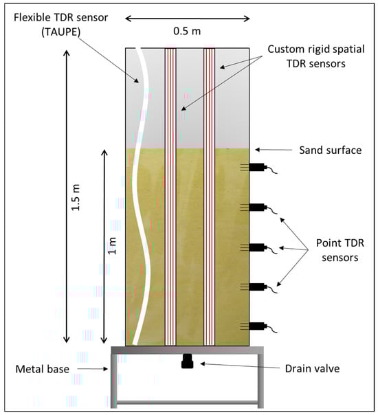
Figure 2.
The vertical installation of custom spatial probes (STDR2, STDR1, and TAUPE) and the horizontal installation of commercial point sensors (TDR1–5) in the column ensures continuous spatial measurements of soil moisture during various wetting and drainage experiments.
During the construction of the two spatial probes, it was decided to insulate the central waveguide of one probe to study its impact on the measurements (Figure S3d, Supplementary Materials). According to the literature, the insulation of the central waveguide reduces signal loss during propagation and facilitates soil moisture estimation in conductive and saline soils [59], but also reduces the sampling volume, which is already limited to a few centimeters around the waveguides. Conversely, the insulation of the two external waveguides, connected to the coaxial cable’s ground, does not affect the measurements. The results of this study justify these findings. The spatial TDR waveguide setups that are used for this experiment are named STDR1 (non-insulated central waveguide) and STDR2 (insulated central waveguide).
After constructing the probe, one end of the waveguides was soldered to a coaxial cable while the other end was left untouched, creating an open electric circuit. The central pin of the coaxial cable was soldered to the central copper wire, while the ground of the cable was soldered to the outer copper wires [60] and the waveguides serve as an extension of the cable (Figure S3e,f, Supplementary Materials). A BNC adapter was attached to the other end of the cable to connect the coaxial cable to a TDR device. During a measurement, the device generates an electromagnetic pulse that travels through the cable and propagates through the waveguides. Next, the device records all pulse reflections along the waveguides that occur where the impedance changes. The impedance depends on the geometry of the probe (the size and spacing of the waveguides) and is inversely related to the dielectric constant of the surrounding medium. A change in soil moisture around the probe alters the soil dielectric constant, which is interpreted as an impedance change and affects the shape of the reflection used for soil moisture estimation.
2.2.3. Custom Flexible Probe (TAUPE)
The second type of custom spatial sensor used in this study to monitor soil moisture changes within the column is a flexible TDR sensor known as TAUPE (Figure 1, Figure 2, and Figure S1c, Supplementary Materials) that has proven to be appropriate for estimating soil moisture profiles [61]. TAUPE is an insulated flexible sensor, in the form of a flat ribbon, developed by the Institute of Meteorology and Climate Research at Forschungszentrum Karlsruhe [8,62,63,64]. TAUPE features three flat copper wires covered with polyethylene and has a sampling volume of 3–5 cm around the waveguides, based on the dielectric constant of the surrounding soil [65]. These sensors exhibit less signal attenuation in the same medium compared to sensors with uninsulated metal waveguides, resulting in increased accuracy. The sensor used in this study is 10 m long.
2.3. Cables and Connectors
To connect the STDR1, STDR2, and TAUPE sensors with the TDR devices, RG-58 C/U 50 Ohm coaxial cables, with a propagation velocity of 66%, were used. Campbell Scientific’s CS645 point sensors use a low-loss LMR-200 50 Ohm coaxial cable, with a propagation velocity of 83%. Such 50 Ohm coaxial cables are widely used in the literature to match the output impedance of TDR devices [66].
The cable length of the STDR1 and STDR2 probes was set at 2 m to minimize signal losses as it propagates along the waveguides and to provide the necessary flexibility. The cable length for the CS645 sensors was set at 3 m, while the cable of the TAUPE sensor measures 10 m. Lastly, BNC male plugs were used to connect the coaxial cables with the TDR devices.
2.4. Measurement Instruments
In this study, the main TDR devices used for soil moisture estimations during the experiments in the artificial column were TDR100 by Campbell Scientific Inc. (Manufacturer: Campbell Scientific Ltd., Loughborough, UK) and HL1101 by Hyperlabs Inc. (Manufacturer: HYPERLABS INC., Beaverton, OR, USA) (Figure S9b, Supplementary Materials). These devices have a 50 Ohm output impedance and generate an electromagnetic pulse that first propagates along the coaxial cable and then through a probe with metal rods that act as an extension of the cable. Next, the reflected waveforms are collected and digitized by the instrument for storage and analysis. Any impedance change will cause the amplitude of the reflected signal to change as well. When the sensor is inserted into the soil, the propagation time of the generated pulse along the waveguides depends on the soil moisture. The higher the moisture content, the longer the propagation time. The reflected waveform can be used to trace the transition of the signal from one material to another due to impedance changes, as well as the start and end of the sensor. Finally, the propagation time and amplitude of the reflected pulse can be used to estimate the soil moisture content.
When multiple sensors were required in this study for water content measurements, a 50 Ohm SDMX50 multiplexer from Campbell Scientific Inc. was used (Manufacturer: Campbell Scientific Ltd., Loughborough, UK), which can receive up to eight TDR sensors or more by connecting multiple multiplexers. As the measurements mainly had to be conducted and stored automatically, an integrated system was developed that included a pulse generator (TDR100), a datalogger (CR800), a multiplexer (SDMX50), a 12V power supply, and a waterproof casing for mounting all components (Figure S9b, Supplementary Materials). The waterproof design allowed the system to be used in the field for several days, as demonstrated in a previous publication. The safe operation of the system was ensured by properly grounding the instruments (Figure S9b, Supplementary Materials). After the automated and continuous storage of all measurements, the raw reflections were processed and converted into soil moisture estimations.
2.5. Software
For water content measurements and troubleshooting during the soil column experiments with the instruments HL1101 and TDR100, the respective software ZTDR Version 2.1.0 by Hyperlabs Inc. and PC-TDR Version 3.0 by Campbell Scientific Inc. were used.
2.6. Quartz Sand and Water Quality Characterization
To better interpret the soil column measurements and the movement of water within the column, a series of laboratory experiments was conducted at the Agricultural University of Athens to determine the soil water retention curve (SWRC) and the saturated hydraulic conductivity of the quartz sand, and to assess the quality of the water used in the column experiments.
To optimize the accuracy of the results during the soil column infiltration experiments, low-conductivity, low-salinity pure quartz sand of river origin was used to fill the column, deliberately avoiding materials such as coastal sands and clays, which are known to potentially distort TDR readings.
2.6.1. Soil Water Retention Curve
The SWRC is like a fingerprint, as each soil has its own. Researchers use these curves to predict and comprehend water movement and storage in a specific type of soil and at a particular soil moisture. A retention curve describes the amount of water retained in the soil under equilibrium conditions at a specific retention potential and presents the relationship between soil moisture and negative pressure [67]. The shape of a retention curve is unique for each soil type and is related to its texture, bulk density, pore size, and connectivity, and is therefore heavily influenced by granulometry and structure, and by other factors including organic matter content [68].
Ref. [69] proved that the relationship between negative pressure (suction) and water content is not described by a single curve, but by two distinct curves, one for the wetting and one for the drainage of the soil. Hence, the drainage–wetting process is not reversible and the difference between the two curves is called hysteresis. Due to the presence of entrapped air during the wetting and drainage of the medium and the geometry of the porous media, the relationship between soil moisture and suction is represented by an infinite number of curves related to the wetting and drainage background of the soil.
Modeling the dispersion and flow of water on partially saturated soils requires knowledge of the SWRC and, therefore, plays a critical role in water management, in calculating water storage and the appropriate irrigation dose, and in predicting the dissolution and transport of pollutants through the vadose zone. Typically, a SWRC is strongly non-linear and it is relatively difficult to achieve accuracy [68].
Various techniques can be used to determine the SWRC of a soil. In this study, the Haines apparatus was utilized to construct the retention curve of the quartz sand due to its simplicity and reliability [69]. Based on the negative pressure heads and the corresponding water content values measured during the application of the method, the SWRC of the sand was created (Figure 3).

Figure 3.
The soil water retention curve of the quartz sand.
2.6.2. Saturated Hydraulic Conductivity
The hydraulic conductivity of a saturated soil determines the ease with which water can move through that soil. In other words, hydraulic conductivity reflects the ability of a porous material, such as soil, to allow water to move through its mass under saturated or near-saturated conditions.
Hydraulic conductivity depends on both soil properties (texture, porosity, structure, compaction, etc.) and water properties (viscosity, temperature, density, etc.). Saturated hydraulic conductivity in the laboratory differs from that in the field because, in the laboratory, the total saturation of the soil sample can be achieved, whereas in the field when wetting occurs from the soil surface, the air cannot escape and is trapped in the soil by the infiltrating water, preventing the soil from reaching full saturation.
Knowledge of this parameter is crucial for estimating the water mass balance and aquifer recharge of the soil under investigation. Hydrologists and researchers need to know this parameter to run their models, assess soil quality, and predict water movement in different parts of the soil, while many agricultural decisions, such as irrigation rates, depend on information like soil erosion potential and nutrient leaching, which depend on this parameter. Ultimately, hydraulic conductivity governs soil water movement.
There are several laboratory and field techniques to measure saturated and unsaturated soil hydraulic conductivity. The constant-head method is suitable for saturated hydraulic conductivity estimations in the laboratory, while single-ring and double-ring infiltrometers are the most common field techniques.
The constant-head method [70] was used in this study to determine the saturated hydraulic conductivity of the quartz sand. The calculated value was 6.664 cm/min.
2.6.3. Water Quality
The water used in the column experiments has an electrical conductivity of 286 μS/cm and a pH of 7.85. The low conductivity of water ensures less signal attenuation and more reliable TDR and GPR results.
2.6.4. Laboratory Environmental Conditions
All experiments were conducted indoors in the laboratory. As a result, the environmental and experimental conditions were limited to standard room conditions. Temperature and humidity were monitored throughout the entire series of experiments, with temperatures ranging from 19.5 °C to 20.5 °C, and humidity was between 40% and 50%. Based on multiple laboratory and field experiments conducted in the past and an extensive literature review, such conditions are highly unlikely to affect the study outcomes or compromise the reliability of measurements for either the TDR or GPR methods. Furthermore, the short duration of the infiltration experiments, combined with the fact that all experiments were conducted during the same time of year, ensured that these environmental conditions remained stable throughout all measurement processes. As a result, all measurements were conducted under consistent conditions.
3. Results
To assess the developed hydrogeophysical system, four series of experiments were conducted. Each series differed in the wetting process and the sensors and techniques used to monitor soil moisture changes within the column. The pros and cons of each sensor and technique are presented below.
3.1. Variable Saturation with Water Input at Different Depths Without Drainage (TDR Measurements)
In the first series, the wetting of the sand was realized from within its mass. An array of irrigation hoses and nozzles was placed in the sand at 10, 50, and 90 cm above the bottom of the column and connected to water supply hoses for a fixed flow of 2 L/min (Figure S5, Supplementary Materials). The drain valve was closed during the inflow and, as a result, 15 min after the start of the flow, a saturated water front formed at the bottom of the column and began to move towards the surface. After the first measurement in dry sand, the next measurements were taken at every 10 cm of upward water movement, at heights of 10, 20, 30, 40, 50, 60, 70, 80, 90, and 100 cm (total saturation) (Figure S6, Supplementary Materials). A TDR waveform was recorded at each height using each point sensor (TDR1, TDR2, TDR3, TDR4, and TDR5) and the STDR1 and STDR2 custom spatial sensors. This type of wetting ensures the total saturation of the sand, as the upward flow of water removes the air and fills the pores with water [71,72,73]. The ease with which the upward flow could be monitored validated the choice of plexiglas as a suitable material for soil column experiments (Figure S6, Supplementary Materials).
After the complete saturation of the sand, the column was drained through the valve at the bottom of the column and measurements were taken with the same sensors every 10 cm of falling water level, i.e., at heights of 90, 80, 70, 60, 50, 40, 30, 20, and 10 cm. After the end of the drainage, the first 10 cm of sand from the bottom remained nearly saturated, mainly due to the fact that the drainage took place through a small opening at the bottom and the presence of the sieve, which increased the adhesion and cohesion between the water molecules, resulting in increased matric and reduced gravitational forces, preventing the expulsion of water. During drainage, the water level was not as visible as during wetting because of the moisture held in the sand above the water level due to capillary forces; however, there were no major problems in conducting measurements at the desired water levels (Figure S7, Supplementary Materials).
In this series, the measurements were conducted with the pulse generator TDR100 so that the multiplexer SDMX50 could be used. All sensors were connected to the multiplexer and measurements for each sensor were taken manually using the PCTDR software, as the time of each measurement depended on the water level.
The reflectograms for all the sensors during the wetting phase are shown in Figure 4, where the propagation of the signal through the different media and the transition from one to the other can be seen. For the custom spatial sensors, STDR1 and STDR2, the first part of the diagram refers to the propagation of the pulse through the coaxial cable; the next part refers to the propagation through the air, as the first 50 cm of the sensors are outside the sand; and the next part corresponds to the propagation of the signal in the sand and is used to estimate soil moisture. The last part of the diagram shows the infinite reflection, which is commonly used to estimate the electrical conductivity of the soil and is beyond the scope of this paper. The reflectograms of the point sensors (TDR1, TDR2, TDR3, TDR4, and TDR5) feature the same parts, but without the air part, as the waveguides of these sensors are only in contact with the sand.
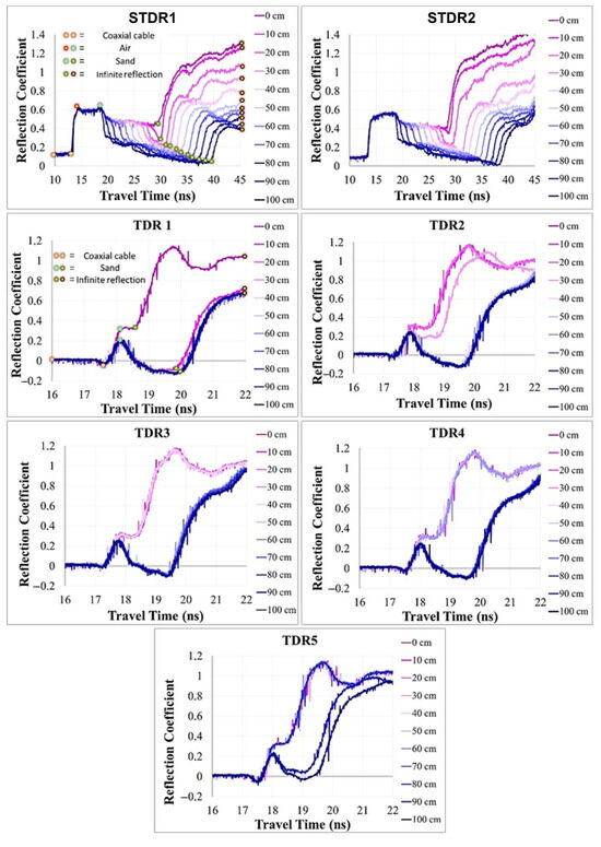
Figure 4.
The reflection coefficient versus travel time graphs for the spatial (STDR1 and STDR2) and point sensors (TDR1, TDR2, TDR3, TDR4, and TDR5) during sand wetting. The legend of each graph shows the water level, where 0 cm is dry sand and 100 cm is complete saturation.
The legend of each graph shows the water level, where 0 cm is dry sand and 100 cm is complete saturation. Each graph shows how the reflection coefficient changes as a function of the water content of the sand. The higher the water content of the sand, the lower the reflection coefficient and the longer the propagation time of the pulse, as the dielectric constant of the sampling volume increases. The graphs of the point sensors do not show the gradual decline that the spatial sensors do as, due to their short length and horizontal installation, they can measure almost exclusively dry or fully saturated sand. An intermediate state is shown for TDR2 and TDR5, indicating that at the time of the measurement one part of the waveguides was in contact with dry sand and the other with saturated sand.
The reflectograms for all the sensors during the drainage phase are shown in Figure 5. The graphs follow the reverse trend compared to wetting, but with some differences. For the STDR1 and STDR2 sensors, the graphs representing the lower water level at 10 cm show lower reflection coefficient values right before the infinite reflection compared to wetting, as this part of the sand remains nearly saturated. The STDR2 sensor shows lower reflection coefficient values at lower water levels compared to the STDR1 sensor, indicating that more water accumulates around the lower parts of this sensor. Overall, the differences between the spatial sensors during both wetting and drainage are not significant, suggesting that under controlled conditions, with homogeneous soil material and low conductivity, the insulation of the central waveguide (STDR2 sensor) has little effect on the quality of the measurements.
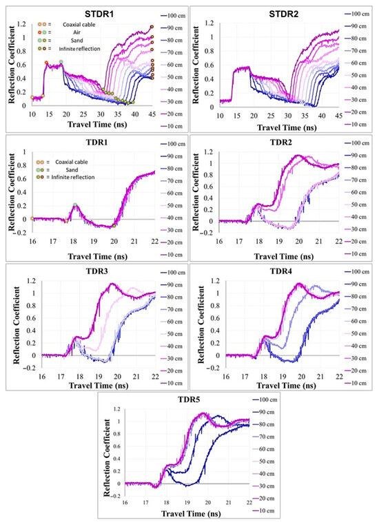
Figure 5.
The reflection coefficient versus travel time graphs for the spatial (STDR1 and STDR2) and point sensors (TDR1, TDR2, TDR3, TDR4, and TDR5) during sand drainage. The legend of each graph shows the downward water level.
The point sensors, due to their short length and orientation, show the same but reversed behavior during drainage compared to wetting, with the only difference being the lack of changes for the TDR1 sensor. This sensor is located at a height of 10 cm, where the sand remains almost saturated after drainage (Figure S7d, Supplementary Materials) and there are no reflection coefficient changes.
The soil moisture profiles for each sensor and water level during both wetting and drainage were calculated from the plots in Figure 4 and Figure 5, using the numerical one-dimensional model by Ref. [53], and considering only the part of the graphs where the signal propagates through the sand. The dielectric constant profiles calculated with this model were then converted to soil moisture profiles using the calibration equation by Ref. [74]. The first 50 cm of the two spatial sensors are outside the sand, in contact only with the air, and cannot be used in soil moisture estimations, as the air has a dielectric constant of around one and the equation by Ref. [74] is only valid for permittivities between 3 and 40.
The estimated soil moisture profiles and values for all sensors during wetting and drainage are shown in Figure 6 and Figure 7. For the point sensors, a mean moisture value was calculated for each plot in Figure 4 and Figure 5. The estimated soil moisture profiles of the STDR1 and STDR2 spatial sensors and the mean values of the point sensors for each water level during wetting are shown in Figure 6. The vertical axis represents the depth of the sand and the waveguide length inside the column, and the horizontal axis, the soil moisture. Each plot represents the soil moisture profile around each spatial sensor for a given water level, while each shape represents the calculated average for a given point sensor and water level. It is noted that the higher the water level, the higher the saturation and soil moisture. It is also noted that the soil moisture in almost dry conditions is between 5% and 6% for the parts of the spatial sensors below 10 cm, while in saturation it ranges between 30% and 31% for the STDR2 sensor and around 35% for the STDR1 sensor. Overall, the moisture values for the STDR2 sensor are reduced compared to those of the STDR1 sensor and show a smaller range for each water level, probably due to the insulation which reduces the sampling volume. In short, the spatial sensors exhibit the same pattern of soil moisture increase and some differentiation in the range of values due to the manufacturing characteristics of the waveguides, such as the insulation of the central waveguide, and the physical position of the sensors in the sand and possible proximity to water hoses, which may slightly reduce the measured permittivity and therefore the measured soil moisture.
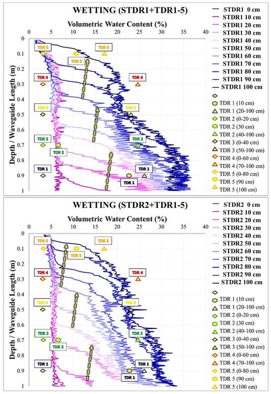
Figure 6.
A comparison between the soil moisture profiles of the custom spatial sensors (STDR1 and STDR2) and the mean values of the point sensors (TDR1, TDR2, TDR3, TDR4, and TDR5) for all rising water levels shown in the legend, during the wetting of the sand.
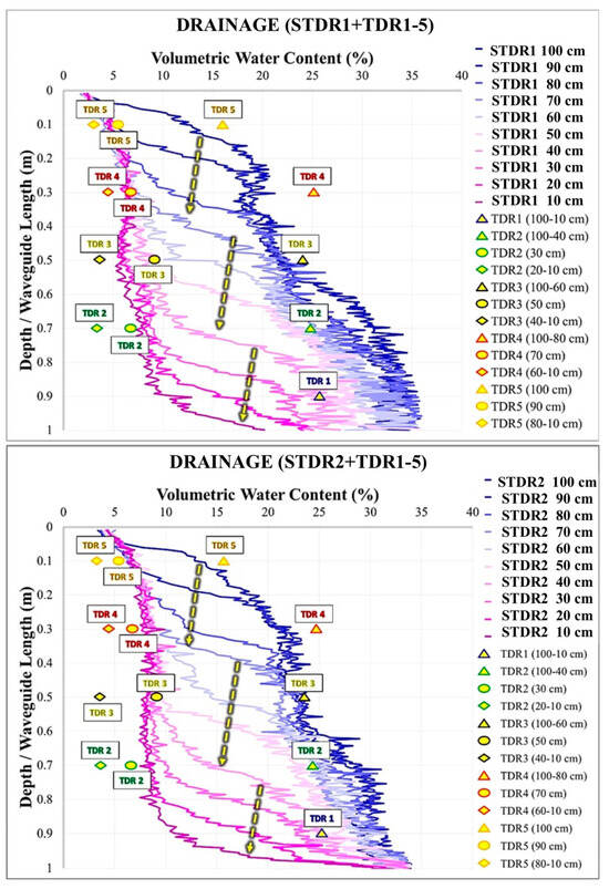
Figure 7.
A comparison between the soil moisture profiles of the custom spatial sensors (STDR1 and STDR2) and the mean values of the point sensors (TDR1, TDR2, TDR3, TDR4, and TDR5) for all falling water levels shown in the legend, during the drainage of the sand.
Figure 6 also shows that the moisture values for the point sensors in dry conditions are around 3% and are lower than the equivalent for the spatial sensors, which range between 5% and 6%. This difference is probably due to the fact that the first 0.5 cm of the waveguides are only in contact with the plexiglas material of the column that is 0.5 cm thick (Figure S2, Supplementary Materials) and has a permittivity of about 3, reducing the overall average soil moisture. In general, the permittivity of dry sand is around 3–4, close to the limit below which the calibration equation by Ref. [74] provides questionable moisture estimates.
In Figure 7, a larger deviation is observed between the lowest soil moisture estimates of the point sensors and the moisture profiles of the spatial sensors at the lowest water level, as a result of the higher moisture retained around the spatial sensors due to greater adhesion forces compared to the much shorter point sensors. However, the average moisture estimates of the TDR2, TDR3, TDR4, and TDR5 sensors, when the water level has reached the installation height of these point sensors, almost perfectly match the lowest moisture values of the STDR1 and STDR2 sensors during drainage.
The estimated soil moisture profiles of the STDR1 and STDR2 spatial sensors and the mean values of the point sensors for each water level during drainage are shown in Figure 7. The lower the water level, the lower the volumetric water content. At the end of drainage, at a water level of 10 cm, the estimated soil moisture for the parts of the spatial sensors above 10 cm is between 5% and 10%, with an average of about 8%, which is higher by 5–6% during wetting for the same water level, due to moisture being retained by capillary forces. The STDR2 sensor also shows a lower range of values compared to the STDR1 sensor during drainage. The consistency of the results between wetting and drainage confirms the effect that the insulation of the central waveguide of the STDR2 sensor has on the measurements. Overall, the plots in Figure 7 are almost the same as those in Figure 6, but in reverse order, with a slight increase in soil moisture at each water level because of the moisture retained in the sand after drainage due to strong matric forces and weak gravitational forces. This means that during wetting, the overlying layer of sand above the rising water level is completely dry, whereas during drainage, the layer of sand above the falling water level retains moisture that cannot be removed by gravity and is held by capillary forces, a situation known as field capacity.
Figure 6 and Figure 7 demonstrate the immediate response of the custom spatial sensors to changes in soil moisture, both for rising and falling water levels, as these changes are recorded at almost the same height as the water level. This immediate response and the very logical moisture estimates are the first proof of the reliable use of these sensors in field studies, under real conditions.
Comparing the results of the spatial and point sensors at various saturation levels is complicated because each type measures different parts of the soil and with a different orientation. Thus, the estimated values of the point sensors and the moisture profiles of the spatial sensors in Figure 6 and Figure 7 can provide a more spatial approach to measuring soil moisture using TDR and an initial quantitative and qualitative estimate of the behavior of the sand around each sensor, but they are not sufficient for a reliable juxtaposition of sensors and evaluation of the STDR1 and STDR2 spatial sensors.
The best method for this evaluation is probably to compare the maximum moisture values estimated for each sensor during wetting and drainage, as shown in Figure 6 and Figure 7, and study their deviation. The results are presented in Table 1. Apart from the TDR5 sensor, which shows lower values at full saturation, all other sensors show very similar values. In fact, the standard deviation between the TDR1, TDR2, TDR3, TDR4, STDR1, and STDR2 sensors is only 1.15% during wetting and 1.01% during drainage. There is a 2–3% deviation between the STDR1 and the point sensors, while the insulated STDR2 sensor almost matches the point sensors. The insulation of the central waveguide of the STDR2 sensor probably generates a narrower range of values than the uninsulated STDR1 sensor, which matches the values of the calibrated point sensors. However, even the slight deviation of the STDR1 sensor is considered normal, as a moisture deviation of up to 3% could be a result of the calibration equation used or some noise during the propagation of the pulse.

Table 1.
The maximum soil moisture estimates for all sensors during the wetting and drainage of the sand.
To compare the results of the STDR1 and STDR2 spatial sensors, the average soil moisture for each plot and water level in Figure 6 and Figure 7 was calculated and the outcome is shown in Figure 8. During wetting, where the overlying layer of sand above the rising water level is completely dry, the STDR1 sensor shows higher values than the STDR2 sensor for all water levels, the maximum deviation though, is no more than 3%. During drainage instead, where the overlying layer retains some moisture, the values of the two sensors overlap in the first 50 cm of the falling water level and only in the last 40 cm does the STDR2 sensor show higher moisture values; however, again, the maximum deviation is only 2.41% at a level of 30 cm. Therefore, the insulation produces a small divergence in moisture estimates when part of the sand is completely dry, but when there is retained moisture, there is no substantial differentiation between the two sensors.
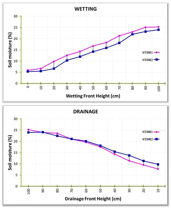
Figure 8.
A comparison between the average moisture estimates for the STDR1 and STDR2 sensors for each water level during wetting and drainage of the sand.
Overall, the divergence between the moisture estimates of the spatial and point sensors does not exceed 2–3%, whether in dry conditions (Figure 6) or in full saturation (Table 1), suggesting that the custom STDR1 and STDR2 spatial sensors performed equally well as the calibrated and high-accuracy point sensors that were selected to calibrate and evaluate the performance of the spatial sensors due to their ability to accurately record even the smallest moisture changes in the surrounding material. Also, the divergence between the moisture estimates of the STDR1 and STDR2 spatial sensors was just as small. In summary, the results of this series are promising and, as will be proven next, are indicative of the potential of the custom spatial sensors, with or without insulation, to be used efficiently in real field studies.
3.2. Variable Saturation with Rainfall Simulation Without Drainage (TDR Measurements)
In this series of column experiments, the column was again filled with dry sand up to a height of 1 m and artificial infiltration was realized by simulating rainfall. A transparent hose in a spiral form, with tiny equidistant openings on the bottom, was placed on top of the column (Figure S8c, Supplementary Materials). The end of the spiral hose was sealed so that water could only enter the sand through the openings. The other end was connected to a valve to supply water and regulate the flow, which, in this experiment, was set at 1.2 L/min. The drainage valve was closed during the water supply and a rising water level appeared sometime after the start of the water inflow. This saturated water front formed at the bottom of the column 25 min after the start of the wetting (Figure 9), indicating an unsaturated hydraulic conductivity of 4 cm/min. The first measurement was conducted in dry sand and the following measurements were taken every 5 min from the start of wetting. The final measurement during wetting took place after 50 min, when the sand was fully saturated (Figure 9). After this time, the sand was drained and the measurements were conducted in the same way as in the first series. After the end of the drainage, the first 10 cm above the bottom of the column remained nearly saturated in this series as well.

Figure 9.
Different saturation phases during sand wetting. At 0 min the sand is completely dry, at 50 min full saturation has been achieved, and at field capacity (FC) the sand has drained and some moisture has been retained due to matric forces.
In this series, the five point sensors (TDR1, TDR2, TDR3, TDR4, and TDR5), the STDR insulated custom spatial sensor, and the flexible insulated TAUPE sensor were used to monitor soil moisture changes during the rainfall simulation (Figure S8b, Supplementary Materials). The point sensors were again used to calibrate and evaluate the STDR and TAUPE sensors.
Although the conditions are also controlled, this series was the first attempt to move closer to natural field processes by simulating rainfall and monitoring induced water flows. An important assumption made for all series of experiments was the absence of preferential flow around the spatial probes. Another type of preferential flow in column experiments occurs on the inner walls of the column [75,76,77] and is the result of improper soil placement inside the column or the bending of the walls after soil placement [9]. Preferential flow can cause spatial heterogeneity in the movement of water and solutes in a porous material and can greatly affect experimental results. Although the assumption of no preferential flow is not correct, it is necessary for calculating infiltration rates in natural systems and for monitoring vadose zone hydrology and water movement. The presence of a foreign body in the soil, such as the spatial sensors, causes preferential flow and its calculation for the correction of infiltration rate values is very cumbersome.
The measurements in this series were conducted with the HL1101 device and Z-TDR software from Hyperlabs Inc. A waveform was measured and stored for each sensor and a full cycle of measurements took almost two minutes since a multiplexer and a datalogger could not be used with this instrument and switching between sensors was performed manually. Therefore, this series not only compares different types of sensors, but also compares different types of instruments.
The different stages of water movement and the different formations from the start of wetting (0 min) to full saturation (50 min) and drainage (FC = Field Capacity) of the sand are shown in Figure 9. During the first phase of wetting, when a saturated front has not yet formed at the bottom of the column, the downward water movement is not uniform. The water follows specific routes and part of the sand remains dry and unaffected by the downward flow. After 25 min though, the saturated front forms at the bottom and moves uniformly upwards until the sand is completely saturated after 50 min. During this time, the rising water front removes the remaining air and the pores are filled with water, gradually saturating the sand.
The paths and formations formed during the first 25 min of wetting have the shape of a sound wave and are known as fingerings (Figure 9), which are formed when there is instability in the water front as it moves through unsaturated coarse soil materials such as sand [78]. Ref. [79] showed that the width of the fingering is a function of grain size, as silt shows formations with a diameter of one meter and coarse sand of just 1 cm. While fingering is mostly observed in sandy materials, the hydrophobia of soil has also been investigated [80,81]. Ref. [78] suggest that the fingering width is generally independent of the flow in the system when the infiltration rate is smaller than the saturated conductivity. As flow increases and reaches the saturated hydraulic conductivity rate, the width and frequency of fingerings will increase until these formations unite on a single saturated front without fingerings. A potential fingering can significantly affect measurements if a constant soil moisture is desired in a soil column experiment. Ref. [82] demonstrated that fingering is more common when wetting a dry soil. Figure 9 confirms findings in the literature, as this experiment shows fingerings in initially dry sandy soil.
The reflectograms for all the sensors during the wetting phase are shown in Figure 10, whereas, in Figure 4, the propagation of the signal through the different media and the transition from one to the other can be seen. The legend of each graph shows the time of each measurement from the start of wetting. The first plot (0 min) represents the measurement in dry sand, before the start of wetting, and the last plot (50 min) represents the measurement in fully saturated sand. The graphs of the STDR and TAUPE sensors show that as wetting progresses and the water content of the sand around the sensors increases, the reflection coefficient decreases and the propagation time of the pulse increases, as the dielectric constant of the sampling volume increases. The propagation times for the TAUPE sensor are greater than the STDR sensor due to the much longer length of the flexible sensor. The graphs for the point sensors in Figure 10 show more reflection coefficient changes than the graphs in Figure 4. This is due to the fact that, in this series for 25 min, there is not a single front affecting the entire length of the waveguides, but many fingerings affecting different parts of the point sensors. The TDR5 sensor, for example, shows a slight gradual increase in travel time for 40 min and an abrupt transition to saturation after 45 min. Such frequent reflection coefficient changes are present in all point sensors, indicating uneven moisture distribution and water movement in the sand.
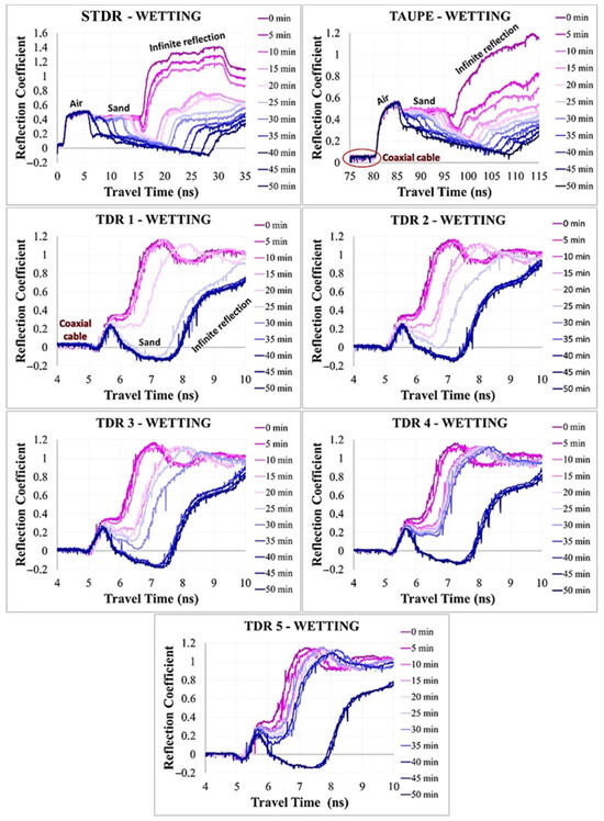
Figure 10.
The reflection coefficient versus travel time graphs for the spatial (STDR and TAUPE) and point sensors (TDR1, TDR2, TDR3, TDR4, and TDR5) during sand wetting. The legend of each graph shows the exact time of the measurement from the start of wetting, where the first plot (0 min) represents the measurement in dry sand, before the start of wetting, and the last plot (50 min) represents the measurement in fully saturated sand.
The reflectograms for the STDR and TAUPE sensors during the drainage phase are shown in Figure 11. The graphs follow the reverse trend compared to wetting because as the sand drains, the reflection coefficient increases and the propagation time of the pulse decreases. Overall, the reflectograms in Figure 11 show a narrower range of values than the wetting in Figure 10 because the overlying sand above the falling water level retains some moisture due to matric forces. After the end of drainage, the graphs representing the lower water level at 10 cm show lower reflection coefficient values right before the infinite reflection compared to wetting, as this part of the sand remains nearly saturated. The STDR sensor shows lower reflection coefficient values at lower water levels compared to the TAUPE sensor, which is probably due to the complete insulation of the TAUPE sensor, which reduces signal loss and the sampling volume of the measurements, as the same trend is observed during wetting. Overall, the STDR and TAUPE spatial sensors show the same patterns of gradual decrease and increase in reflection coefficient during wetting and drainage, respectively, with some slight differences. To better evaluate these two spatial sensors, the corresponding soil moisture profiles were estimated.

Figure 11.
The reflection coefficient versus travel time graphs for the STDR and TAUPE spatial sensors during sand drainage. The legend of each graph shows the falling water level.
The soil moisture profiles for each sensor during both wetting and drainage were calculated from the plots in Figure 10 and Figure 11 in the same way as in the previous series, using the model by Ref. [53] and the calibration equation by Ref. [74], considering only the parts of the graphs where the signal propagates through the sand.
The estimated soil moisture profiles of the STDR and TAUPE spatial sensors and the mean values of the point sensors for each timestamp during wetting are shown in Figure 12. It is noted that the soil moisture in dry conditions (0 min) is around 4–5% for the STDR and TAUPE sensors, while at full saturation (50 min) the maximum value is around 34% for the STDR sensor and 36% for the TAUPE sensor. Between these two states there is a constant increasing trend in the moisture profiles, which is not as symmetrical as in Figure 6. This is probably due to the fact that, as mentioned above, the saturation of the sand is not uniform during the first part of the wetting process and the water formations created and moving downwards affect the different parts of the sensors unevenly. Even after the formation of the saturated front, which begins to move upward after the first 25 min, the changes in soil moisture profiles between 25 and 50 min are still not uniform, possibly due to variable saturated areas in the overlying sand above the water level, causing some areas to reach full saturation faster than others.

Figure 12.
A comparison between the estimated soil moisture profiles of the custom spatial sensors STDR and TAUPE and the mean values of the point sensors (TDR1, TDR2, TDR3, TDR4, and TDR5) from the start (0 min) to the end of the wetting and full saturation of the sand (50 min).
Figure 12 also shows that the mean moisture values of all the point sensors in dry conditions are around 3% and are similar to those of the spatial sensors in dry conditions. In fact, in the case of the TAUPE sensor, they are almost identical.
Overall, the TAUPE sensor shows the maximum soil moisture values, around 36%, but the STDR sensor shows higher overall values and a wider range of values at almost all depths. These differences may be the result of the complete insulation of all the waveguides of the TAUPE sensor, which reduces the sampling volume of the measurements, whereas in the STDR sensor only the central waveguide is insulated. In short, the two spatial sensors exhibit a similar pattern of soil moisture increase and some differentiation in the range of values due to the manufacturing characteristics of the waveguides and their different insulation, possibly due to the physical position of the sensors in the sand and the influence of variable saturated areas during wetting.
The estimated soil moisture profiles of the STDR and TAUPE spatial sensors and the mean moisture values of the point sensors for each water level during drainage are shown in Figure 13. As the drainage progresses and the water level falls, the water content decreases. At the end of the drainage, where the soil has reached field capacity, the moisture above 20 cm ranges between 5% and 10% for both spatial sensors. These values are greater than the 4–5% during wetting because some moisture is retained in the sand due to matric forces. Below 20 cm, the moisture increases rapidly and almost reaches saturation for the STDR sensor as this part of the sand retains water mainly due to the presence of the screen. At field capacity, there is a significant difference between the moisture values for the TDR2, TDR3, TDR4, and TDR5 point sensors and the values for the STDR and TAUPE spatial sensors. This is probably due to the larger surface area and greater adhesion of water to the walls of the spatial sensors around the waveguides, which increases the moisture estimated. In addition, the spatial sensors are affected by the surrounding and variably saturated sand along their entire length, which increases the average soil moisture at field capacity, as shown in the soil moisture profiles. Conversely, the mean moisture value of the TDR1 point sensor at field capacity is almost identical to the values of the STDR and TAUPE sensors.
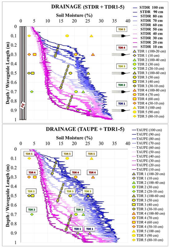
Figure 13.
A comparison between the soil moisture profiles of the STDR and TAUPE custom spatial sensors and the mean values of the point sensors (TDR1, TDR2, TDR3, TDR4, and TDR5) for all falling water levels shown in the legend during the drainage of the sand.
The soil moisture plots of the TAUPE sensor during drainage (Figure 13) show a narrower range of values and lower absolute values at the same height than the STDR sensor. This agrees with the results during wetting (Figure 12), validating the greater effect that the insulation of all the waveguides of the TAUPE sensor has on the signal compared to the STDR sensor, where only the central waveguide is insulated.
In short, apart from an abrupt soil moisture decrease between 70 cm and 60 cm of the water level for the STDR sensor, the progression of the soil moisture profiles during drainage is rather uniform because, unlike wetting, the measurements were conducted at equal spatial intervals of water level drop and the saturated and overlying unsaturated sand layers are also uniform.
Figure 12 and Figure 13 show the capacity of the STDR and TAUPE custom spatial sensors to capture even the smallest soil moisture changes during wetting and drainage of the sand under controlled conditions, with some small deviations between their values, further suggesting their efficient implementation in real field conditions.
As in the previous series, the best way to evaluate the performance of the spatial sensors and compare it with that of the point sensors is probably to compare the maximum moisture values estimated for each sensor during wetting and drainage, as shown in Figure 12 and Figure 13, and to study their deviation. The results are presented in Table 2. The values are similar and the maximum deviation between all sensors is less than 3%. In fact, the standard deviation between all sensors is only 0.92% during wetting and 0.88% during drainage. The maximum deviation between the STDR and point sensors is less than 1.5% throughout the experiment and between the TAUPE and point sensors is less than 3%. The results indicate that the STDR and TAUPE spatial sensors performed equally well as the calibrated point sensors.
Table 2.
The maximum soil moisture estimates for all sensors during wetting and drainage of the sand.
Overall, based on Table 2, which compares the values for all sensors at full saturation, and Figure 12, which shows nearly identical values for all sensors under dry conditions, it can be deduced that the maximum deviation between all sensors and saturation levels is always less than 3%. This is considered normal, as a moisture deviation of up to 3% could be the result of the calibration equation used or noise during the propagation of the pulse and cannot be easily avoided.
To compare the results of the STDR and TAUPE spatial sensors, the average soil moisture for each plot and water level of Figure 12 and Figure 13 was calculated and the outcome is shown in Figure 14. During the first 15 min of wetting, the STDR sensor shows slightly larger values, while during the next 15 min, the values of the two sensors are identical. From that point onward, the TAUPE sensor shows higher values, although the largest difference, after 35 min, is only 2.6%. During drainage, a similar pattern is observed; in the first half, the TAUPE sensor shows slightly larger values, while in the second half, the STDR sensor exhibits the same behavior. The largest deviation occurs at the end of drainage, at a water level of 10 cm, and is only 1.4%. Overall, these small differences are likely the result of the non-uniformity of soil moisture around the various parts of the sensors and the different types of insulation. However, they are small enough to suggest that either sensor could replace the other without compromising measurement integrity.
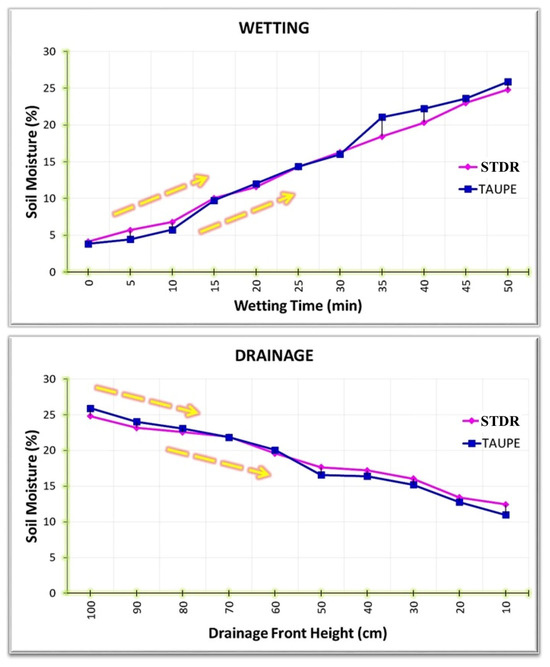
Figure 14.
A comparison between the average moisture estimates for the STDR and TAUPE sensors during wetting and drainage of the sand.
In summary, the second series of column experiments confirms the results of the first series regarding the measurement integrity of the custom spatial sensors. All deviations between the moisture estimates from the spatial and point sensors, as well as between the STDR and TAUPE sensors, for all saturation levels, do not exceed 3%, suggesting that all spatial sensors, with or without insulation, can be effectively used in field studies. In addition, the divergence between the moisture estimates of all sensors in the first and second series is also less than 3%, as shown by Figure 6, Figure 7, Figure 12, and Figure 13. This data indicates that the two different pulse generator devices used in these series can provide comparable integrity in soil moisture measurements.
3.3. Variable Saturation with Rainfall Simulation with Drainage (TDR and GPR Measurements)
In the third series of column experiments, artificial infiltration was achieved by simulating rainfall in the same way as in the second series. The same transparent spiral hose was placed at the top of the column and connected to a valve to supply water and regulate the flow, which, in this experiment, was set at 0.75 L/min. In this series, however, the drainage valve was open during the water supply so that the water balance could be calculated. Hence, an attempt was made to simulate an actual aquifer recharge process by calculating the amount of water infiltrating and draining from the sand.
The duration of wetting was 62 min, after which the valve was left open to allow all available water to drain from the sand due to gravitational forces. When the field capacity was reached, the valve was closed and a new phase of wetting began with the same flow, creating a rising saturated front that eventually led to the full saturation of the sand.
In this series, the measurements were conducted using the TDR and GPR methods and a qualitative comparison between the two methods was attempted. GPR was selected due to its ability to measure larger soil volumes quickly and because its function is based on the same principles as TDR. Each method complements the other, as they both depend on the permittivity and electrical conductivity of the soil. A typical GPR system consists of an antenna that emits a high-frequency electromagnetic wave into the soil and an antenna that receives and measures the amplitude of the reflected wave as a function of time. The propagation velocity of the waves is mostly dependent on the permittivity of the soil, which in turn is influenced by soil moisture.
The selection of the GPR method played a crucial role in determining the parameters for this series of experiments. The water flow was reduced from 1.2 L/min in the previous series to 0.75 L/min in this series, allowing for the more efficient tracing of water movement and moisture changes. The process of rising water levels was also implemented here to evaluate GPR performance under saturated conditions. The wetting time was limited to one hour, as the previous series indicated no significant changes in water flow after that time.
For the TDR method, the five point sensors and the STDR spatial sensor were used in this series. The point sensors were connected to the multiplexer, which was connected to the TDR100 pulse generator. These two devices were then connected to the CR800 datalogger for the automated storage of the measurements every two minutes. In this series, a mean moisture value was automatically calculated for each point sensor during the experiment by importing the appropriate code into the datalogger. A 12V battery powered the system, which was grounded with some quartz sand (Figure S9b, Supplementary Materials). The STDR sensor measurements were taken manually with the HL1101 device, also every two minutes. The complete TDR system used in this series is shown in Figure S9b, Supplementary Materials.
For GPR measurements, two high-density paper guides (Figure S9a, Supplementary Materials) were installed on the external walls of the column to avoid interference with electromagnetic waves from the device. The measurements were taken with the Ramac Proex device from MALA GEOSCIENCE (Manufacturer: Guideline Geo AB (publ), Solna, Sweden) with a 1.6 GHz shielded antenna (Figure S9d, Supplementary Materials). For each measurement, the device moved slowly downward, starting from a height of 120 cm and ending at the bottom of the column (Figure 15). This downward movement was selected to initially avoid the effect of the metal base of the column on the measurements and to better image the water flow processes during wetting of the sand. The first measurement was taken in dry sand, while subsequent measurements were conducted at two-minute intervals until the end of wetting, just like with TDR. Next, a measurement at field capacity was taken using both methods. Finally, after closing the valve and resuming wetting, measurements were taken at every 10 cm of rising water level, as in the first two series.

Figure 15.
(Left) Snapshot from the GPR measurements during the wetting of the sand. (Right) The column setup for the GPR measurements as designed in Blender, a free and open-source 3D creation suite.
From the start of wetting, the first drop of water fell into the container below the column (Figure S9c, Supplementary Materials) after 16 min, indicating a sand infiltration rate of 6.25 cm/min, which is very close to the saturated hydraulic conductivity of 6.664 cm/min calculated with the constant-head method. This value suggests that the effect of preferential flow along the walls of the spatial sensors is probably not that significant.
Based on the fixed water flow of 0.75 L/min and the wetting time, it can be easily calculated that a total of 46.5 L of water infiltrated the sand during the 62 min of wetting. After wetting ended and drainage ceased, allowing the sand to reach field capacity, the total volume of drained water was measured at 29 L, which means that approximately 17.5 L remained in the sand due to capillary forces and negative pore pressure. This approach of the free drainage of pore water from the bottom of the column without applying suction is quite common in the literature (e.g., Refs. [11,14,15,21,22,83,84,85,86,87]. Due to simultaneous free drainage during wetting, the sand did not reach full saturation while the valve remained open. Instead, because the sand is initially dry, the infiltrating water forms specific paths (fingerings) that it tends to follow. As wetting progresses, the number and size of these formations increases (Figure S10, Supplementary Materials).
The soil moisture values for the point sensors during wetting, with and without drainage, are shown in Figure 16. These values were automatically calculated using the appropriate program loaded into the datalogger. This image shows a gradual increase in moisture values for all sensors during wetting, which depends on the position of each sensor in the column. The TDR1 sensor shows the greatest increase, although during the first 26 min it is not much affected by the infiltrating water, as the moisture change does not exceed 1.5%. However, after the 28th minute, there is an abrupt increase that reaches almost 18%. The TDR2 sensor shows the greatest increase after the TDR1 sensor from the 28th minute, but with much lower values, with a maximum of less than 10%, followed by the TDR3 sensor. The TDR5 sensor, located very close to the surface, shows the highest values until the 26th minute, which is rather reasonable as it is the first to be affected by the infiltrating water. However, there is no significant increase in soil moisture after that time, indicating that only a small amount of additional water has accumulated around this sensor. The same behavior is also witnessed for the TDR4 sensor. Overall, the results suggest that during wetting, more water accumulates near the bottom of the column, as the soil tends to retain less water at greater heights due to stronger gravitational and weaker matric forces.
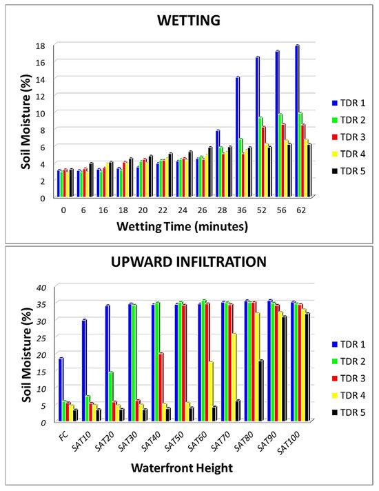
Figure 16.
The automatically calculated soil moisture values for the point sensors during wetting, with (top image) and without (bottom image) drainage.
The bottom image of Figure 16 shows the soil moisture changes for the point sensors during the subsequent wetting phase, this time without drainage, as water levels rise from field capacity (FC) to full saturation of the sand (SAT100). Each sensor is affected by the rising water level, showing an abrupt increase in moisture, before the water level reaches the sensor’s height, likely due to capillary rise. The TDR3 sensor, for example, shows a premature moisture increase at 40 cm of water level and then, at 50 cm, which is the placement height for this sensor, the next big rise occurs, leading to full saturation. The maximum moisture values at full saturation fluctuate around 35% for the TDR1, TDR2, and TDR3 sensors, whereas the TDR4 and TDR5 sensors show lower values of 33% and 31.8%, respectively. At field capacity, the TDR1 sensor records 18.5% moisture due to water accumulation near the bottom, while the other four sensors record much lower values, ranging between 3.3% and 5.8%.
The automatically calculated values of the point sensors in Figure 16 align reasonably well with the values of the point sensors calculated in the previous two series using the numerical model and the calibration equation described earlier.
The reflectograms for the STDR sensor during wetting, with (top image) and without drainage (bottom image), are shown in Figure 17. The legend of the top image represents the time of each measurement from the start of wetting at dry sand (0 min) until the end of wetting (62 min). The legend of the lower image indicates the level of the rising water (SAT) and the thickness of the overlying sand layer in field capacity (FC). Hence, FC represents the measurement taken after the end of drainage, at field capacity, while SAT70FC30 refers to the measurement when the first 70 cm from the bottom are saturated, and the remaining 30 cm of the overlying sand are at field capacity.

Figure 17.
The reflection coefficient versus travel time graphs for the STDR spatial sensor during sand wetting with (top image) and without drainage (bottom image). The legend of the top image represents the time of each measurement, from the start (0 min) to the end of wetting (62 min), while the lower image shows the level of the saturated front (SAT) and the thickness of the overlying sand layer in field capacity (FC).
During the entire wetting with drainage process (0–62 min), only the lower parts of the sensor, near the bottom, seem to be gradually affected by the infiltrating water. This indicates that the water mainly followed specific paths to exit through the bottom, without significantly affecting the sampling volume of the upper parts. This does not rule out the possibility of preferential flow around the sensor, which may have occurred on the opposite side, 6 cm away from the waveguides, thereby avoiding entering the sensor’s sampling volume. On the contrary, after re-wetting without drainage (FC-SAT100FC0), significant changes in the reflection coefficient are observed. As the wetting progresses and saturation increases, the reflection coefficient decreases, and the travel time increases due to the higher permittivity values of the soil surrounding the sensor.
The soil moisture profiles for the STDR sensor during wetting, with and without drainage, were calculated from the plots in Figure 17 using the same numerical model and calibration equation as in the previous series, considering only the sections of the plots where the signal propagates through the sand. The results are shown in Figure 18, where a comparison between the soil moisture profiles from the STDR sensor and the automatically calculated values from the point sensors is presented, offering a more spatial approach to imaging soil moisture changes during wetting. The point sensors are significantly more affected by the infiltrating water than the STDR sensor, showing a greater range of values at each height, especially during wetting with drainage (top image), where the parts of the STDR sensor at depths shallower than 90 cm present little variation, which increases at greater depths. Significant soil moisture changes for the STDR sensor during wetting with drainage are shown only in the first 10 cm above the bottom, where the moisture gradually increases, reaching a maximum value of 17.3% after 56 min. The plots for 56 and 62 min are nearly identical, indicating that if wetting continued beyond 62 min, there would be no significant changes in moisture. Above this height, the moisture is relatively constant, at around 4.5–6%, with a slight increase noticed only between 0.4 and 0.5 cm of height after 56 min.

Figure 18.
A comparison between the calculated soil moisture profiles from the STDR spatial sensor and the automatically calculated values from the point sensors (colorful shapes) during wetting, with (top image) and without drainage (bottom image).
The lowest moisture for the point sensors in dry sand is approximately 3%, while for the STDR sensor, it ranges between 4% and 5%. Conversely, after 62 min of wetting, the maximum values for the STDR and TDR1 sensors are almost identical, at around 18%.
A relatively uniform upward trend in soil moisture profiles is observed during wetting without drainage (bottom image), except for an abrupt increase between 30 cm and 40 cm of rising water level. This is probably due to variably saturated parts of the overlying sand above the water level, causing some areas to reach saturation faster than others. The maximum calculated moisture value for the STDR sensor at full saturation is 36.1%, while at field capacity before rewetting, it ranges from 3% to 5%. Cumulatively, the plots in Figure 18 tally with those in Figure 12 for the STDR sensor, as the wetting process is the same. The 0–10 min section in Figure 12 aligns with the 0–62 min section in Figure 18. The time difference is due to different water flow rates between the two series. The figures illustrating moisture changes during the upward movement of water show the same pattern of moisture change and the same abrupt increase between 0.4 and 0.6 cm in height. The maximum value for the STDR sensor is approximately 34% in Figure 12 and 36% in Figure 18, which is an acceptable deviation.
The bottom image in Figure 18 shows the moisture changes during the rewetting of the sand without simultaneous drainage. The maximum values for the STDR sensor at heights of 10 cm and 30 cm above the bottom almost coincide with the maximum values for the TDR1 and TDR2 sensors. Above this height, the maximum values of the spatial sensor decline. This is probably because the first 50 cm of the sensor are outside the sand, causing the gradual increase in soil moisture until the maximum value is reached. Similarly, the lowest values at field capacity for the point sensors and STDR sensor nearly coincide, except for the TDR1 sensor. The TDR1 sensor value at field capacity is roughly 18%, which differs significantly from the STDR sensor value at 10 cm, around 5%, indicating that the sand surrounding the TDR1 sensor is wetter than the corresponding area around the STDR sensor. Overall, the maximum soil moisture values for all sensors during wetting, with and without drainage, are presented in Table 3.
Table 3.
The maximum soil moisture values for all sensors during wetting, with and without drainage.
The results of the GPR measurements in dry sand are shown in Figure 19. This map of signal reflections highlights parts of the column setup that produce stronger reflections, such as the spatial sensors, the opposite side of the column and the metal base beneath the column. The sand and the air above it are also visible, along with the impact of signal transition between the two materials, which is indicated by stronger reflections at their interface. The white-gray areas within the sand section indicate a lack of reflections, primarily representing dry sand. However, after the start of wetting, the results were insufiicient to generate maps that effectively track water movement and soil moisture changes within the sand.
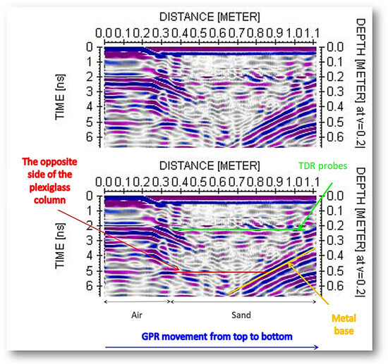
Figure 19.
The results of the GPR measurement in dry sand. This map displays the signal reflections, indicating the different parts of the column setup.
The two main causes of this failure were likely the curvature of the column and the movement of infiltrating water along the inner walls of the column, which increased electrical conductivity near the device. These factors caused significant dispersion and attenuation of the electromagnetic signal, reducing the resolution of the measurements within the moist sand. A possible solution to obtain better results would be the separation of signals in the time domain, which would only be valid if stronger contrasts existed. The creation of a 3D model using the degree of curvature and the column material as input data could also be used to analyze signal propagation both in the air and in the sand. Another option would be to use a column of a different size, or the same-sized column with GPR antennas of varying frequencies. A different, yet complex and demanding approach with uncertain outcomes would be the use of frequency filters to cut or boost specific frequencies and separate the different signals. All these approaches could be of some benefit, but because they require time and research for better results, they are not part of this study. The approach used for the successful application of the GPR method in the column during the wetting of the sand is presented in the next chapter.
Overall, in this series, an experiment was conducted that more closely approached real-field conditions compared to the first two series, as the wetting of the sand was realized with simultaneous free drainage to avoid full saturation and estimate the water mass balance. In this third series, the soil moisture changes within the sand were also monitored using a more spatial approach with both spatial and point TDR sensors. The accuracy of these spatial sensors was assessed and validated during the first three series, indicating that the TDR method can be used not only for point measurements but also for soil moisture estimation in larger soil volumes and deeper parts of the vadose zone using multiple spatial sensors, even with varying orientations. The GPR method did not provide satisfactory results in this series; however, by analyzing these failures, the experiment in the next chapter was designed.
3.4. Variable Saturation with Point Rainfall Simulation with Drainage (GPR Measurements)
For efficient GPR measurements in the column during the wetting of the sand, it was decided to change the wetting process rather than the shape of the column. A successful GPR application with this approach could pave the way for future curved column measurements, which may face serious signal dispersion issues. To reduce the combined effect of curvature and increased conductivity near the GPR device, produced by water movement along the inner walls, the wetting in this series was applied only above the center surface of the sand (Figure S11, Supplementary Materials). Hence, the spatial sensors were removed, dry sand was added up to one meter, and a custom setup was installed above the center of the sand to simulate point rainfall. By doing so, the GPR signal reflections and preferential flow produced by the spatial sensors were eliminated. The infiltrating water now moves naturally through the sand and preferential flow may occur only along the inner walls of the column.
The wetting duration was 80 min and the valve remained open the entire time to allow all available water to drain from the sand due to gravitational forces and to calculate the mass balance of the water entering and exiting the sand. This duration was based on the results from the previous two series, which indicated that no substantial differences would occur after that time. The water flow was reduced and fixed at 0.3 L/min to allow GPR to more efficiently map water movement and soil moisture changes throughout the experiment.
In this series, measurements were taken solely with the GPR method, using the same device and the same downward motion on the outer walls of the column (Figure S11, Supplementary Materials) as in the previous series. Measurements were taken at two-minute intervals, from the first measurement in dry sand to the last at the end of wetting after 80 min. No measurements were taken after the end of wetting.
From the start of wetting, the first drop of water fell into the container below the column after 24 min, indicating a natural sand infiltration rate, without preferential flow, of 4.16 cm/min. Based on the fixed water flow of 0.3 L/min and the wetting time, it was calculated that a total of 24 L of water infiltrated the sand during the 80 min wetting period. After wetting ended and drainage ceased, allowing the wetted parts of the sand to reach field capacity, the total volume of drained water was measured at 10.5 L, indicating that approximately 13.5 L remained in the sand due to capillary forces and negative pore pressure.
Because of free drainage, the sand cannot reach full saturation during wetting. Specific pathways (fingerings) are created, as mentioned earlier, that the infiltrating water tends to follow until it exits the sand from the bottom of the column (Figure S11, Supplementary Materials). Contrary to the previous two series, the fingerings in this series do not appear at the surface. Instead, they first appear after 10 min in the lower half of the sand, with their size and number increasing as wetting progresses. After 16 min, the first sign of water appears at the bottom, while after 30 min, a uniform saturated front has already formed just above the bottom. After that time, and until the end of wetting at 80 min, the saturated front did not significantly increase in size. Between 10 and 80 min, several formations of varying size and shape appeared at different depths in the lower half of the sand. The last image (150 min) shows that, 70 min after the end of wetting, the formations have increased in size due to the capillary movement of water in the sand pores.
In Figure 20, the resulting 2D amplitude envelope maps of selected GPR measurements during wetting are shown. The horizontal axis represents the distance traveled by the GPR device at each measurement, from a height of 120 cm to the bottom of the column. The left vertical axis represents the signal propagation time, while the right axis, the surveying depth. In this study, the depth is approximately 0.5 m due to the high frequency of the antenna used (1.6 GHz). The first measurement (0 min) was conducted in dry sand and the last one was taken after 80 min, when the wetting process was complete. The purple color indicates areas with many reflections, while the gray color represents areas with few reflections. This happens because the gray areas have higher electrical conductivity values, which lead to greater signal attenuation and therefore, fewer reflections.
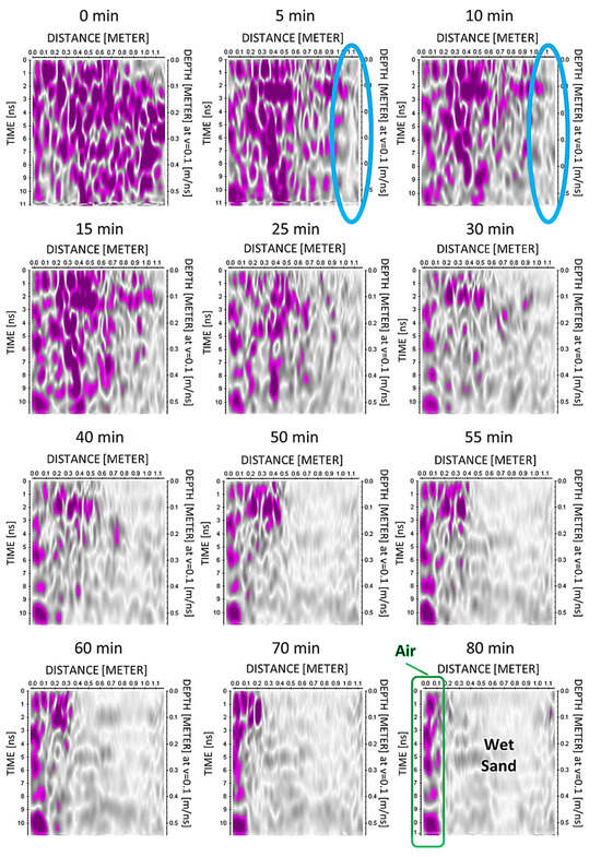
Figure 20.
The resulting 2D amplitude envelope maps of selected GPR measurements from the start (0 min) until the end of wetting (80 min). The blue elliptical shapes indicate a conductive area, which could represent either the saturated front just above the bottom, observed in all series, or the impact from the metal base. In the final map (80 min), the air above the sand surface (purple area) and the variably saturated sand (gray area) are shown.
The first image (0 min) shows the dry sand and the map is filled with reflections (purple areas) due to the resistive nature of the dry sand. This image serves as a reference point to help interpret the subsequent maps during the wetting process. As the wetting progresses and the water content in the sand increases, the reflections (purple areas) gradually decrease, while the conductive areas (gray color) expand, indicating that water has infiltrated these areas, increasing their conductivity, which, in turn, attenuates the signal and reduces the number of reflections.
Within just 5–10 min of wetting, a conductive area has already formed just above the bottom (elliptical blue shapes), indicating either the saturated front observed in that part of the column in all series or the metal base beneath the column. This gray front expands and moves towards the surface as the wetting progresses, due to the increasing saturation of the sand. After 80 min of wetting, the two materials (air and sand) through which the signal propagates can be clearly seen. At the start of a GPR measurement, the device is positioned 120 cm above the bottom (Figure 15) and part of the waves propagate through the air above the sand surface, which is represented as a fixed purple area in all images with a thickness of more than 10 cm. This is clearly seen in the final image (80 min) in Figure 20. When the device moves below 100 cm, the main part of the signals propagates through the variable saturated sand. Initially, this is represented by purple areas due to the dry sand and gradually it converts into gray areas as wetting progresses.
The GPR results are not as accurate as the TDR results; however, the application of the GPR method in this series is considered successful, as it managed to map the general movement of water and how the sand is affected by the infiltrating water during an extended period of wetting. Although Figure S11 (Supplementary Materials) shows that the sand has not reached full saturation during wetting, the maps in Figure 20, especially those after 50 min, indicate nearly full saturation. This likely occurs due to the presence of saturated sand near the device, which causes attenuation of the signal and, as a result, weaker propagation to the sand, making it difficult to image possible dry areas on the other side of the column. As seen in Figure S11 (Supplementary Materials), the main wetted formations appear near the wall where the GPR measurements are taken and the high electrical conductivity of these areas further attenuates the propagating waves. However, considering the curvature of the column, which makes the measurements even more challenging, the results are satisfactory. The use of low conductivity water (286 μS/cm) was proven successful because, with high conductivity water, the attenuation of the signal would be greater, and the results would likely be unusable, as seen in the previous series. Overall, the results from this series demonstrate the ability of the GPR method to effectively monitor water movement in a controlled column experiment under appropriate conditions and highlight the potential of this monitoring system to be used on a larger scale for similar hydrological studies.
4. Discussion and Conclusions
Monitoring the deeper parts of the unsaturated zone remains an important problem and new approaches need to be developed in this direction. In this work, an integrated hydrogeophysical system comprising TDR and GPR has been developed and tested under controlled conditions through a series of laboratory column experiments with different wetting and drainage approaches. The primary purpose of these experiments was to evaluate and validate the system for potential application in the field under real conditions.
In this study, several custom spatial TDR sensors, both rigid and flexible, were constructed and tested. The results indicate that these sensors perform as well as commercial calibrated point sensors. Their ability to reliably measure soil moisture changes suggests that they, along with the TDR technique in general, can be used not only for point estimation of soil moisture but also for monitoring moisture changes and hydrological processes in larger soil volumes and deeper parts of the vadose zone using multiple spatially distributed long sensors, with varying orientations as well.
Initially, the performance of the GPR method was limited due to the curvature of the column and signal dissipation caused by the presence of conductive materials near the GPR device. By analyzing these initial shortcomings and minimizing the sources of signal attenuation and dissipation within the column, a new series of measurements was designed, where the GPR technique succeeded in imaging the general water movement and soil moisture changes during sand wetting. Although GPR is less accurate than TDR, it can capture soil water movement and be used for large-scale hydrological studies under specific conditions.
This integrated approach to soil moisture monitoring, combining custom spatial TDR sensors with point sensors and the GPR method, represents the main novelty of the present study.
Overall, the successful combined application of GPR and TDR in the column experiments of this study under controlled conditions and varying wetting and drainage regimes, demonstrates that this system can effectively capture water movement in the soil in a spatial and 3D manner, not only in the laboratory but also in the field under real conditions. Based on the results of this study and the advantages and limitations of the methods, a field infiltration experiment was designed to monitor the hydrology of the unsaturated zone under real conditions at depths greater than a few centimeters from the soil surface using GPR, TDR, and ERT. This experiment is thoroughly described in a previously published paper.
Supplementary Materials
The following supporting information can be downloaded at: https://www.mdpi.com/article/10.3390/w17132003/s1, Figure S1: (a) The plexiglass column and the metal base on which the column was placed. Both the base and the bottom of the column have a hole for the installation of the drainage valve. (b) Before each experiment, the column was filled with dry sand to a height of one meter (c) The sieve at the bottom of the column prevents sand leakage during drainage. (d) The drainage valve; Figure S2: The three-waveguide point sensors (above) used in this study were mounted horizontally on the column; Figure S3: (a) A sample of an HDPE tube featuring surface dikes for the installation of copper wires and a threaded screw for connection to other tubes. (b) Copper spool. (c) The process of gluing copper wires to the grooves of the tube. (d) The central waveguide in the STDR tube is insulated. (e,f) The central pin of the coaxial cable is soldered to the central copper wire, while the ground of the cable is soldered to the outer copper wires; Figure S4: The flexible TAUPE sensor; Figure S5: The wetting setup consists of external water supply hoses and thinner irrigation hoses with nozzles (red circles) placed in the sand at a height of 10, 50 and 90 cm. The 7 sensors were connected to the SDMX50 multiplexer and the measurements were conducted manually using the TDR100 instrument and PCTDR software; Figure S6: The gradual saturation of the sand during the wetting phase; Figure S7: The gradual drainage of the sand. The water level (yellow arrows) is not as visible as during wetting because of the moisture held above the water level due to capillary forces; however, there were no problems in conducting measurements at the desired water levels; Figure S8: (a,b) The setup of the 2nd series of column experiments comprising the five point sensors (TDR1–5), the STDR insulated custom spatial sensor and the flexible insulated TAUPE sensor, as seen from outside (a) and inside the column (b). (c) The transparent spiral hose placed on top of the column to simulate rainfall; Figure S9: (a) The third series column setup with external paper guides for the downward GPR device movement. (b) The complete TDR system for soil moisture measurements with the point sensors comprising a pulse generator (1), a multiplexer (2), a datalogger (3), a 12V power supply (4), and a ground point. The STDR sensor measurements were taken manually using a different pulse generator (5) and associated software (6) (c) A snapshot of the drainage process during wetting (d) The 1.6 GHz device used for GPR measurements; Figure S10: (a) The third series column setup with external paper guides for the downward GPR device movement. (b) The complete TDR system for soil moisture measurements with the point sensors comprising a pulse generator (1), a multiplexer (2), a datalogger (3), a 12V power supply (4), and a ground point; Figure S11: The custom wetting setup installed above the center of the sand surface (0 min) and selected snapshots from the start (0 min) to the end of wetting (80 min). The last image (150 min) shows the water movement due to capillary forces, 70 min after the wetting process ended.
Author Contributions
Conceptualization, A.P. and A.K.; methodology, A.P., G.A., M.T. and A.K.; validation, A.P. and M.T.; formal analysis, A.P.; investigation, A.P., G.A., P.K., M.T. and A.K.; resources, I.A., G.A. and A.K.; data curation, A.P., G.A., I.A., M.T. and A.K.; writing—original draft preparation, A.P.; writing—review and editing, A.P. and A.K.; visualization, A.P., G.A., M.T., A.K. and I.A.; supervision, A.K.; project administration, A.K.; funding acquisition, A.K. All authors have read and agreed to the published version of the manuscript.
Funding
This research was funded by the Special Account for Research Funding (E.L.K.E.) of National Technical University of Athens (N.T.U.A.) and MARSOL—Demonstrating Managed Aquifer Recharge as a Solution to Water Scarcity and Drought (An Environment 2013 Cooperation Project funded by European Union’s Seventh Programme for research, technological development, and demonstration under grant agreement No [619120]).
Data Availability Statement
Dataset available on request from the authors.
Acknowledgments
The authors would also like to thank Dipl-Ing Franz Königer, Head of High-frequency Technology & Sensors, Karlsruhe Institute of Technology (KIT) for providing the TAUPE sensor. The authors would also like to acknowledge the contribution of PhD student Stavros Karizonis, a mining and metallurgical engineer and member of the Applied Geophysics Laboratory of the School of Mining and Metallurgical Engineering at the National Technical University of Athens (NTUA), for his work during the GPR measurements of this study. This research was conducted as part of A.P.’s doctoral thesis at the Laboratory of Engineering Geology & Hydrogeology, School of Mining and Metallurgical Engineering, National Technical University of Athens, Greece.
Conflicts of Interest
The authors declare no conflicts of interest.
References
- Jones, S.; Blonquist, J., Jr.; Robinson, D.; Rasmussen, V.; Or, D. Standardizing Characterization of Electromagnetic Water Content Sensors Part 1. Methodology. Vadose Zone J. 2005, 4, 1048–1058. [Google Scholar] [CrossRef]
- Dahan, O.; McDonald, E.V.; Young, M.H. Flexible Time Domain Reflectometry Probe for Deep Vadose Zone Monitoring. Vadose Zone J. 2003, 2, 270–275. [Google Scholar] [CrossRef]
- Xie, S.; Zhao, G. Study on Spatiotemporal Transport Characteristics of Soil Moisture in Layered Heterogeneous Vadose Zone Based on HYDRAS-3D. Water 2023, 15, 3550. [Google Scholar] [CrossRef]
- Shen, Z.; Yang, Y.; Fu, X.; Adams, K.H.; Biondi, E.; Zhan, Z. Fiber-optic seismic sensing of vadose zone soil moisture dynamics. Nat. Commun. 2024, 15, 6432. [Google Scholar] [CrossRef]
- Hendrickx, J.; Flury, M. Uniform and Preferential Flow Mechanisms in the Vadose Zone. In Conceptual Models of Flow and Transport in the Fractured Vadose Zone; National Academies Press: Washington, DC, USA, 2001; pp. 149–187. [Google Scholar]
- Kallioras, A.; Khan, A.; Piepenbrink, M.; Pfletschinger, H.; Königer, F.; Dietrich, P.; Schüth, C. Time-domain reflectometry probing systems for the monitoring of hydrological processes in the unsaturated zone. Hydrogeol. J. 2016, 24, 1297–1309. [Google Scholar] [CrossRef]
- Oostrom, M.; Dane, J.H.; Wietsma, T.W. A review of multidimensional, multifluid, intermediate-scale experiments: Flow behavior, saturation imaging, and tracer detection and quantification. Vadose Zone J. 2005, 6, 610–637. [Google Scholar] [CrossRef]
- Pfletschinger, H.; Engelhardt, I.; Piepenbrink, M.; Königer, F.; Schuhmann, R.; Kallioras, A.; Schüth, C. Soil column experiments to quantify vadose zone water fluxes in arid settings. Environ. Earth Sci. 2012, 65, 1523–1533. [Google Scholar] [CrossRef]
- Lewis, J.; Sjöstrom, J. Optimizing the experimental design of soil columns in saturated and unsaturated transport experiments. J. Contam. Hydrol. 2010, 115, 1–13. [Google Scholar] [CrossRef]
- Voegelin, A.; Barmettler, K.; Kretzschmar, R. Heavy metal release from contaminated soils: Comparison of column leaching and batch extraction results. J. Environ. Qual. 2003, 32, 865–875. [Google Scholar] [CrossRef]
- Mali, N.; Urbanc, J.; Leis, A. Tracing of water movement through the unsaturated zone of a coarse gravel aquifer by means of dye and deuterated water. Environ. Geol. 2007, 51, 1401–1412. [Google Scholar] [CrossRef]
- Ahmad, R.; Katou, H.; Kookana, R.S. Measuring sorption of hydrophilic organic compounds in soils by an unsaturated transient flow method. J. Environ. Qual. 2005, 34, 1045–1054. [Google Scholar] [CrossRef] [PubMed]
- Rockhold, M.L.; Yarwood, R.R.; Niemet, M.R.; Bottomley, P.J.; Selker, J.S. Experimental observations and numerical modeling of coupled microbial and transport processes in variably saturated sand. Vadose Zone J. 2005, 4, 407–417. [Google Scholar] [CrossRef]
- Branham, B.; Wehner, D.; Torello, W.; Turgeon, A. A microecosystem for fertilizer and pesticide fate research. Agron. J. 1985, 77, 176–180. [Google Scholar] [CrossRef]
- de Jonge, H.; de Jonge, L.W.; Blicher, B.; Moldrup, P. Transport of di(2-ethylhexyl)phthalate (DEHP) applied with sewage sludge to undisturbed and repacked soil columns. J. Environ. Qual. 2002, 31, 1963–1971. [Google Scholar] [CrossRef]
- Batterman, S.; Padmanabham, I.; Milne, P. Effective gas-phase diffusion coefficients in soils at varying water content measured using a one-flow sorbent based technique. Environ. Sci. Technol. 1996, 30, 770–778. [Google Scholar] [CrossRef]
- Seol, Y.; Lee, L.S. Coupled effects of treated effluent irrigation and wetting–drying cycles on transport of triazines through unsaturated soil columns. J. Environ. Qual. 2001, 30, 1644–1652. [Google Scholar] [CrossRef]
- Lewis, J.; Martel, R.; Thiboutot, S.; Ampleman, G.; Trepanier, L. Quantifying the transport of energetic materials in unsaturated sediments from cracked unexploded ordnance. J. Environ. Qual. 2009, 38, 2229–2236. [Google Scholar] [CrossRef]
- Clay, D.E.; Zheng, Z.; Liu, Z.; Clay, S.A.; Trooien, T.P. Bromide and nitrate movement through undisturbed soil columns. J. Environ. Qual. 2004, 33, 338–342. [Google Scholar] [CrossRef]
- Guber, A.K.; Shelton, D.R.; Pachepsky, Y.A. Transport and retention of manure-borne coliforms in soil. Vadose Zone J. 2005, 4, 828–837. [Google Scholar] [CrossRef]
- Aronsson, P.G.; Bergstrom, L.F. Nitrate leaching from lysimeter-grown short-rotation willow coppice in relation to N-application, irrigation and soil type. Biomass Bioenergy 2001, 21, 155–164. [Google Scholar] [CrossRef]
- Colman, E.; Hamilton, E. The San Dimas Lysimeters; U.S. Forestry Service: Berkeley, CA, USA, 1947. [Google Scholar]
- Heimovaara, T.J.; Freijer, J.I.; Bouten, W. The application of TDR in laboratory column experiments. Soil Technol. 1993, 6, 261–272. [Google Scholar] [CrossRef]
- De la Hire, P. Sur L’origine Des Rivières; L’Academie Royale des Sciences: Paris, France, 1703; pp. 1–6. [Google Scholar]
- Darcy, H. Les Fontaines Publiques De La Ville De Dijon: Exposition Et Application Des Principes a Suivre Et Des Formules a Employer Dans Les Questions De Distribution D’eau; Bibliothèque municipale Dijon: Dijon, France, 1856. [Google Scholar]
- Dalton, J. Experiments and Observations to Determine Whether the Quantity of Rain and Dew is Equal to the Quantity of Water Carried off by the Rivers and Raised by Evaporation; Manchester Literary and Philosophical Society: Manchester, UK, 1802; pp. 360–372. [Google Scholar]
- Lawes, J.; Gilbert, J.; Warington, R. On the Amount and Composition of the Rain and Drainage Water Collected at Rothamstead; William Clowes and Sons, Ltd.: London, UK, 1882. [Google Scholar]
- Christiansen, J.E. Effect of entrapped air upon the permeability of soils. Soil Sci. 1944, 58, 355–365. [Google Scholar] [CrossRef]
- Fireman, M. Permeability measurements on disturbed soil samples. Soil Sci. 1944, 58, 337–353. [Google Scholar] [CrossRef]
- Kirkham, D.; Feng, C.L. Some tests of the diffusion theory, and laws of capillary flow, in soils. Soil Sci. 1948, 67, 29–40. [Google Scholar] [CrossRef]
- Brooks, R.H.; Corey, A.T. Hydraulic Properties of Porous Media, Hydrol. Paper No. 3; Colorado State University: Fort Collins, CO, USA, 1964. [Google Scholar]
- van Genuchten, M.T. A closed-form equation for predicting the hydraulic conductivity of unsaturated soils. Soil Sci. Soc. Am. J. 1980, 44, 892–898. [Google Scholar] [CrossRef]
- Liu, C.M.; Zhang, X.Y.; Zhang, Y.Q. Determination of daily evaporation and evapotranspiration of winter wheat and maize by large-scale weighing lysimeter and micro-lysimeter. Agric. For. Meteorol. 2002, 111, 109–120. [Google Scholar] [CrossRef]
- Sahoo, D.C.; Madhu, M.; Khola, O.P.S. Estimation of evapotranspiration and crop co-efficient of carrot (Daucus carota) for water management using weighing lysimeter. Indian J. Agric. Sci. 2009, 79, 968–971. [Google Scholar]
- Hrapovic, L.; Sleep, B.E.; Major, D.J.; Hood, E.D. Laboratory study of treatment of trichloroethene by chemical oxidation followed by bioremediation. Environ. Sci. Technol. 2005, 39, 2888–2897. [Google Scholar] [CrossRef]
- Dontsova, K.M.; Yost, S.L.; Simunek, J.; Pennington, J.C.; Williford, C.W. Dissolution and transport of TNT, RDX, and Composition B in saturated soil columns. J. Environ. Qual. 2006, 35, 2043–2054. [Google Scholar] [CrossRef]
- Sililo, O.T.N.; Tellam, J.H. Fingering in unsaturated zone flow: A qualitative review with laboratory experiments on heterogeneous systems. Groundwater 2000, 38, 865–871. [Google Scholar] [CrossRef]
- Mooney, S.; Morris, C. Quantification of preferential flow in undisturbed soil columns using dye tracers and image analysis. In Proceedings of the SuperSoil 2004: 3rd Australian New Zealand Soils Conference, Sydney, Australia, 5–9 December 2004. [Google Scholar]
- Klein, M.; Müller, M.; Dust, M.; Görlitz, G.; Gottesbüren, B.; Hassink, J.; Kloskowski, R.; Kubiak, R.; Resseler, H.; Schäfer, H.; et al. Validation of the pesticide leaching model PELMO using lysimeter studies performed for registration. Chemosphere 1997, 35, 2563–2587. [Google Scholar] [CrossRef]
- Butler, A.; Chen, J.; Aguero, A.; Edlund, O.; Elert, M.; Kirchner, G.; Raskob, W.; Sheppard, M. Performance assessment studies of models for water flow and radionuclide transport in vegetated soils using lysimeter data. J. Environ. Radioact. 1999, 42, 271–288. [Google Scholar] [CrossRef]
- Koestel, J.; Kemna, A.; Javaux, M.; Binley, A.; Vereecken, H. Quantitative imaging of solute transport in an unsaturated and undisturbed soil monolith with 3-D ERT and TDR. Water Resour. Res. 2008, 44. [Google Scholar] [CrossRef]
- Corey, J.C.; Nielsen, D.R.; Kirkham, D. Miscible displacement of nitrate through soil columns. Soil Sci. Soc. Am. J. 1967, 31, 497–501. [Google Scholar] [CrossRef]
- van der Pol, R.M.; Wierenga, P.J.; Nielsen, D.R. Solute movement in a field soil. Soil Sci. Soc. Am. J. 1977, 41, 10–13. [Google Scholar] [CrossRef]
- De Smedt, F.; Wauters, F.; Sevilla, J. Study of tracer movement through unsaturated sand. J. Hydrol. 1986, 85, 169–181. [Google Scholar] [CrossRef]
- Vanderborght, J.; Vanclooster, M.; Timmerman, A.; Seuntjens, P.; Mallants, D.; Kim, D.; Jacques, D.; Hubrechts, L.; Gonzalez, C.; Feyen, J.; et al. Overview of inert tracer experiments in key Belgian soil types: Relation between transport and soil morphological and hydraulic properties. Water Resour. Res. 2001, 37, 2873–2888. [Google Scholar] [CrossRef]
- Javaux, M.; Vanderborght, J.; Kasteel, R.; Vanclooster, M. Threedimensional modeling of the scale-and flow rate-dependency of dispersion in a heterogeneous unsaturated sandy monolith. Vadose Zone J. 2006, 5, 515–528. [Google Scholar] [CrossRef]
- Mallants, D.; Vanclooster, M.; Meddahi, M.; Feyen, J. Estimating solute transport in undisturbed soil columns using timedomain reflectometry. J. Contam. Hydrol. 1994, 17, 91–109. [Google Scholar] [CrossRef]
- Javaux, M.; Vanclooster, M. Scale- and rate-dependent solute transport within an unsaturated sandy monolith. Soil Sci. Soc. Am. J. 2003, 67, 1334–1343. [Google Scholar] [CrossRef]
- Peters, A.; Durner, W. Improved estimation of soil water retention characteristics from hydrostatic column experiments. Water Resour. Res. 2006, 42. [Google Scholar] [CrossRef]
- Naka, A.; Yasutaka, T.; Sakanakura, H.; Kalbe, U.; Watanabe, Y.; Inoba, S.; Takeo, M.; Inui, T.; Katsumi, T.; Fujikawa, T.; et al. Column percolation test for contaminated soils: Key factors for standardization. J. Hazard. Mater. 2016, 320, 326–340. [Google Scholar] [CrossRef] [PubMed]
- Kalbe, U.; Berger, W.; Simon, F.-G.; Eckardt, J.; Christoph, G. Results of interlaboratory comparisons of column percolation tests. J. Hazard. Mater. 2007, 148, 714–720. [Google Scholar] [CrossRef]
- Meza, S.L.; Kalbe, U.; Berger, W.; Simon, F.-G. Effect of contact time on the release of contaminants from granular waste materials during column leaching experiments. Waste Manag. 2010, 30, 565–571. [Google Scholar] [CrossRef]
- Todoroff, P.; Luk, J.-D.L.S. Calculation of in situ soil water content profiles from TDR signal traces. Meas. Sci. Technol. 2000, 12, 27. [Google Scholar] [CrossRef]
- Papadopoulos, A.; Apostolopoulos, G.; Kallioras, A. An Integrated Hydrogeophysical Approach for Unsaturated Zone Monitoring Using Time Domain Reflectometry, Electrical Resistivity Tomography and Ground Penetrating Radar. Water 2024, 16, 2559. [Google Scholar] [CrossRef]
- Lide, D.R. (Ed.) CRC Handbook of Chemistry and Physics; CRC Press: Boca Raton, FL, USA, 1996. [Google Scholar]
- Telford, W.M.; Geldart, L.P.; Sheriff, R.E. Applied Geophysics, 2nd ed.; Cambridge University Press: New York, NY, USA, 1990. [Google Scholar]
- Dalton, F.N. Development of time-domain reflectometry for measuring soil water content and bulk soil electrical conductivity. In Advances in Measurement of Soil Physical Properties: Bringing Theory into Practice; Topp, G.C., Reynolds, W.D., Green, R.E., Eds.; SSSA special publication; Soil Science Society of America: Madison, WI, USA, 1992; Volume 30, pp. 143–167. [Google Scholar]
- Zegelin, S.J.; White, I.; Russell, G.F. A critique of the time domain reflectometry technique for determining field soil-water content. In Advances in Measurement of Soil Physical Properties: Bringing Theory into Practice; Topp, G.C., Ed.; SSSA special publication; Soil Science Society of America: Madison, WI, USA, 1992; pp. 187–208. [Google Scholar]
- Noborio, K. Measurement of soil water content and electrical conductivity by time domain reflectometry: A review. Comput. Electron. Agric. 2001, 31, 213–237. [Google Scholar] [CrossRef]
- Zegelin, S.J.; White, I.; Jenkins, D.R. Improved field probes for soil-water content and electrical conductivity measurement using time-domain reflectometry. Water Resour. Res. 1989, 25, 2367–2376. [Google Scholar] [CrossRef]
- Scheuermann, A.; Huebner, C.; Schlaeger, S.; Wagner, N.; Becker, R.; Bieberstein, A. Spatial time domain reflectometry and its application for the measurement of water content distributions along flat ribbon cables in a full-scale levee model. Water Res. 2009, 45. [Google Scholar] [CrossRef]
- Schlaeger, S. A fast TDR-inversion technique for the reconstruction of spatial soil moisture content. Hydrol. Earth Syst. Sci. 2005, 9, 481–492. [Google Scholar] [CrossRef]
- Stacheder, M.; Königer, F.; Schuhmann, R. New Dielectric Sensors and Sensing Techniques for Soil and Snow Moisture Measurements. Sensors 2009, 9, 2951–2967. [Google Scholar] [CrossRef] [PubMed]
- Schlaeger, S. Inversion Von TDR-Messungen Zur Rekonstruktion Räumlich Verteilter Bodenphysikalischer Parameter; Institut für Bodenmechanik und Felsmechanik: Karlsruhe, Germany, 2002. [Google Scholar]
- Schlaeger, S.; Becker, R.; Schadel, W.; Scheuermann, A.; Worsching, H. Improvements of Spatial-TDR for Hydrological and Geotechnical Applications. In Proceedings of the 3rd International Symposium and Workshop on Time Domain Reflectometry for Innovative Soils Applica-tions, Purdue University, West Lafayette, IN, USA, 17–20 September 2006; Paper ID 31. p. 19. [Google Scholar]
- Robinson, D.A.; Jones, S.B.; Wraith, J.M.; Or, D.; Friedman, S.P. A Review of Advances in Dielectric and Electrical Conductivity Measurement in Soils Using Time Domain Reflectometry. Vadose Zone J. 2003, 2, 444–475. [Google Scholar] [CrossRef]
- Childs, E.C. The use of soil moisture characteristics in soil studies. Soil Sci. 1940, 50, 239–252. [Google Scholar] [CrossRef]
- Tuller, M.; Or, D. Hydraulic Functions for Swelling Soils: Pore Scale Considerations. J. Hydrol. 2003, 272, 50–71. [Google Scholar] [CrossRef]
- Haines, W.B. Studies in the physical properties of soils. The hysteresis effect in capillary properties and the modes of moisture distribution associated therewith. J. Agric. Sci. 1930, 20, 97–116. [Google Scholar] [CrossRef]
- Klute, A.; Dirksen, C. Hydraulic conductivityand diffusivity: Laboratory methods. In Methods of SoilAnalysis: Part 1—Physical and Mineralogical Methods; Klute, A., Ed.; American Society of Agronomy: Madison, WI, USA, 1986; pp. 687–734. [Google Scholar]
- Casey, F.X.M.; Ewing, R.P.; Horton, R. Automated system for miscible displacement through soil of multiple volatile organic compounds. Soil Sci. 2000, 165, 841–847. [Google Scholar] [CrossRef]
- Jin, Y.; Yates, M.V.; Thompson, S.S.; Jury, W.A. Sorption of viruses during flow through saturated sand columns. Environ. Sci. Technol. 1997, 31, 548–555. [Google Scholar] [CrossRef]
- Liu, P.W.G.; Whang, L.M.; Yang, M.C.; Cheng, S.S. Biodegradation of diesel-contaminated soil: A soil column study. J. Chin. Inst. Chem. Eng. 2008, 39, 419–428. [Google Scholar] [CrossRef]
- Topp, G.C.; Davis, J.L.; Annan, A.P. Electromagnetic Determination of Soil Water Content: Measurements in Coaxial Transmission Lines. Water Resour. Res. 1980, 16, 574–582. [Google Scholar] [CrossRef]
- Corwin, D.L. Evaluation of a simple lysimeter-design modification to minimize sidewall flow. J. Contam. Hydrol. 2000, 42, 35–49. [Google Scholar] [CrossRef]
- Ghodrati, M.; Chendorain, M.; Chang, Y.J. Characterization of macropore flow mechanisms in soil by means of a Split Macropore Column. Soil Sci. Soc. Am. J. 1999, 63, 1093–1101. [Google Scholar] [CrossRef]
- Sentenac, P.; Lynch, R.; Bolton, M. Measurement of the side-wall boundary effect in soil columns using fibre-optics sensing. Int. J. Phys. Model. Geotech. 2001, 4, 35–41. [Google Scholar] [CrossRef]
- Selker, J.S.; Keller, C.K.; McCord, J.T. Vadose Zone Processes; Lewis: Boca Raton, FL, USA, 1999. [Google Scholar]
- Parlange, J.-Y.; Glass, R.; Steenhuis, T. Application of scaling to the analysis of unstable flow. In Scaling in Soil Physics: Principles and Applications, Chap. 5; Hillel, D., Elrick, D., Eds.; Soil Science Society of America Special Publication: Madison, WI, USA, 1990; Volume 25, pp. 53–57. [Google Scholar]
- Bauters, T.W.J.; DiCarlo, D.A.; Steenhuis, T.S.; Parlange, J.Y. Preferential flow in water-repellent sands. Soil Sci. Soc. Am. J. 1998, 62, 1185–1190. [Google Scholar] [CrossRef]
- Ritsema, C.J.; Nieber, J.L.; Dekker, L.W.; Steenhuis, T.S. Stable or unstable wetting fronts in water repellent soils—Effect of antecedent soil moisture content. Soil Tillage Res. 1998, 47, 111–123. [Google Scholar] [CrossRef]
- Liu, Y.P.; Bierck, B.R.; Selker, J.S.; Steenhuis, T.S.; Parlange, J.Y. High intensity X-ray and tensiometer measurements in rapidly changing preferential flow-fields. Soil Sci. Soc. Am. J. 1993, 57, 1188–1192. [Google Scholar] [CrossRef]
- Akhtar, M.S.; Steenhuis, T.S.; Richards, B.K.; McBride, M.B. Chloride and lithium transport in large arrays of undisturbed silt loam and sandy loam soil columns. Vadose Zone J. 2003, 2, 715–727. [Google Scholar] [CrossRef]
- Derby, N.E.; Knighton, R.E.; Montgomery, B.R. Construction and performance of large soil core lysimeters. Soil Sci. Soc. Am. J. 2002, 66, 1446–1453. [Google Scholar] [CrossRef]
- Pasteris, G.; Werner, D.; Kaufmann, K.; Hohener, P. Vapor phase transport and biodegradation of volatile fuel compounds in the unsaturated zone: A large scale lysimeter experiment. Environ. Sci. Technol. 2002, 36, 30–39. [Google Scholar] [CrossRef]
- Rousseau, M.; Di Pietro, L.; Angulo-Jaramillo, R.; Tessier, D.; Cabibel, B. Preferential transport of soil colloidal particles: Physicochemical effects on particle mobilization. Vadose Zone J. 2004, 3, 247–261. [Google Scholar] [CrossRef]
- Troxler, J.; Zala, M.; MoenneLoccoz, Y.; Keel, C.; Defago, G. Predominance of nonculturable cells of the biocontrol strain Pseudomonas fluorescens CHA0 in the surface horizon of large outdoor lysimeters. Appl. Environ. Microbiol. 1997, 63, 3776–3782. [Google Scholar] [CrossRef]
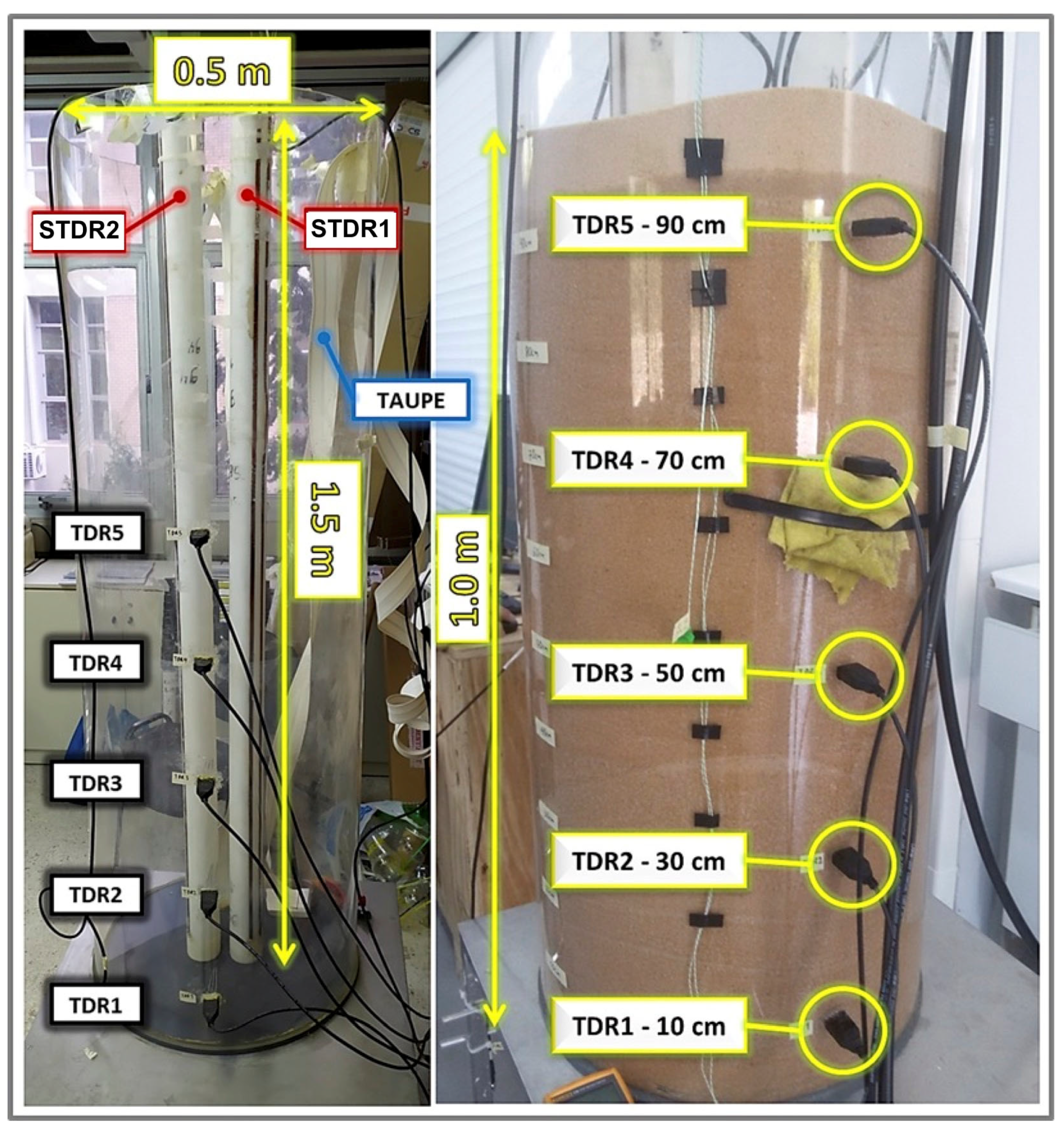

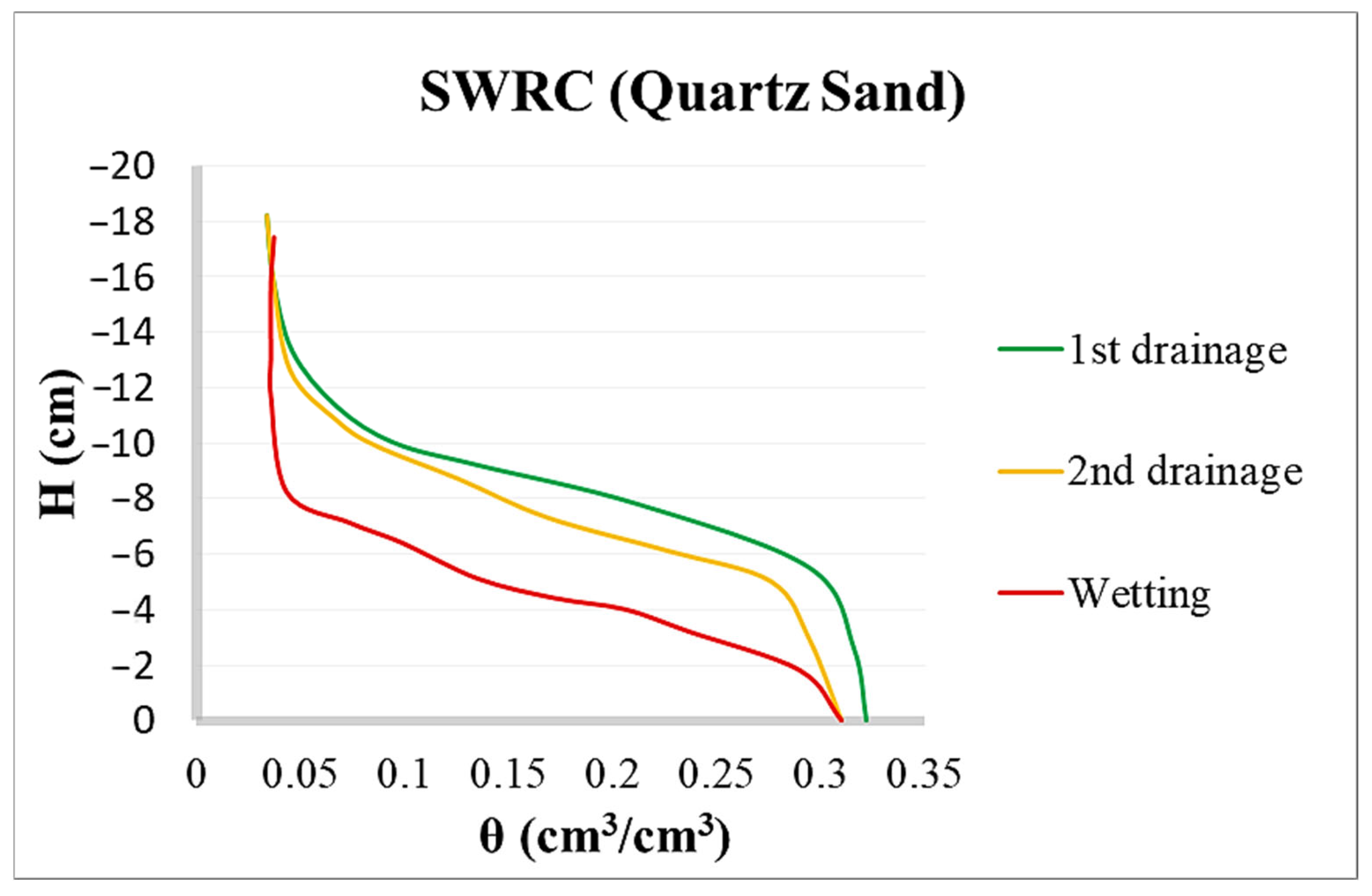
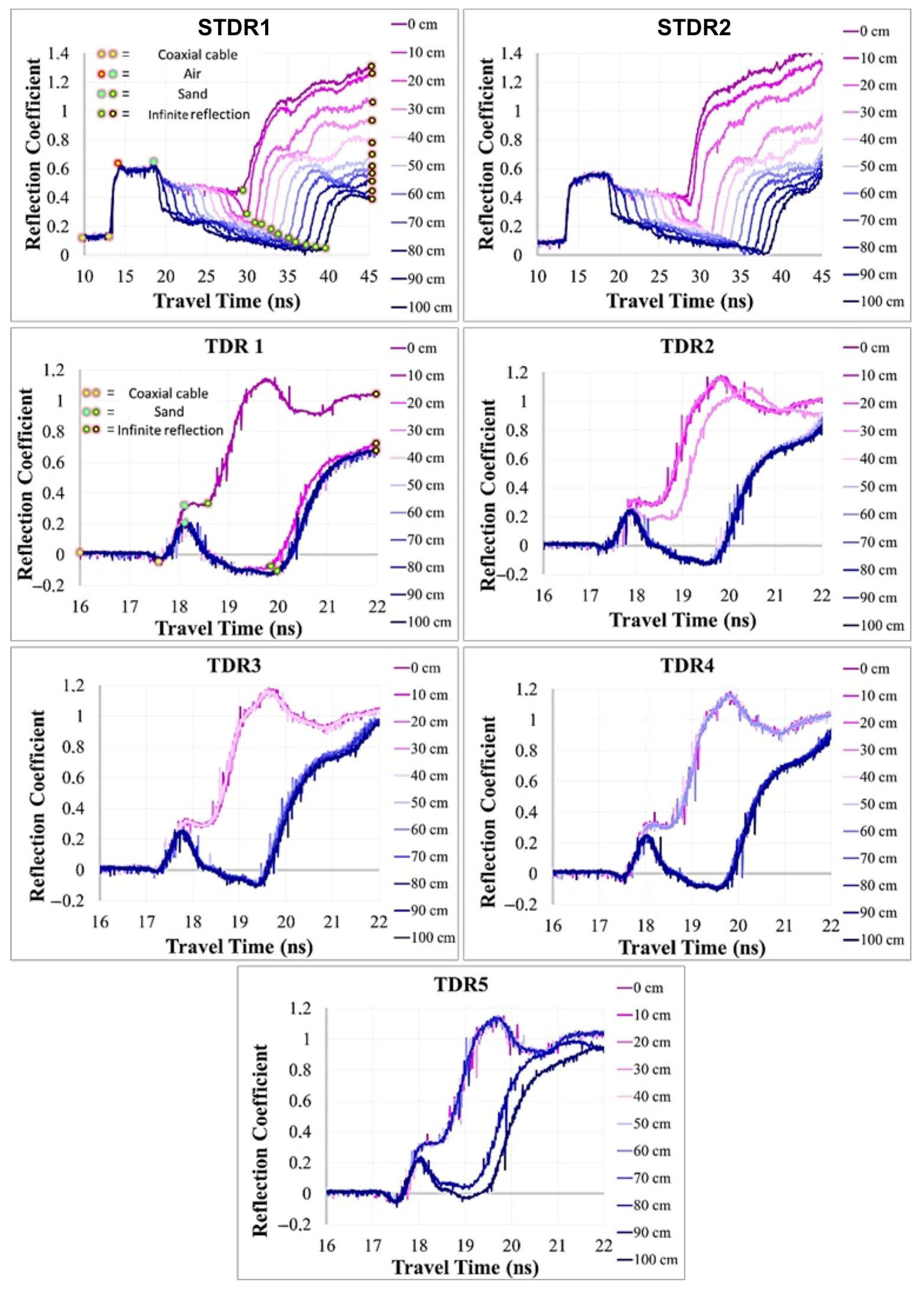
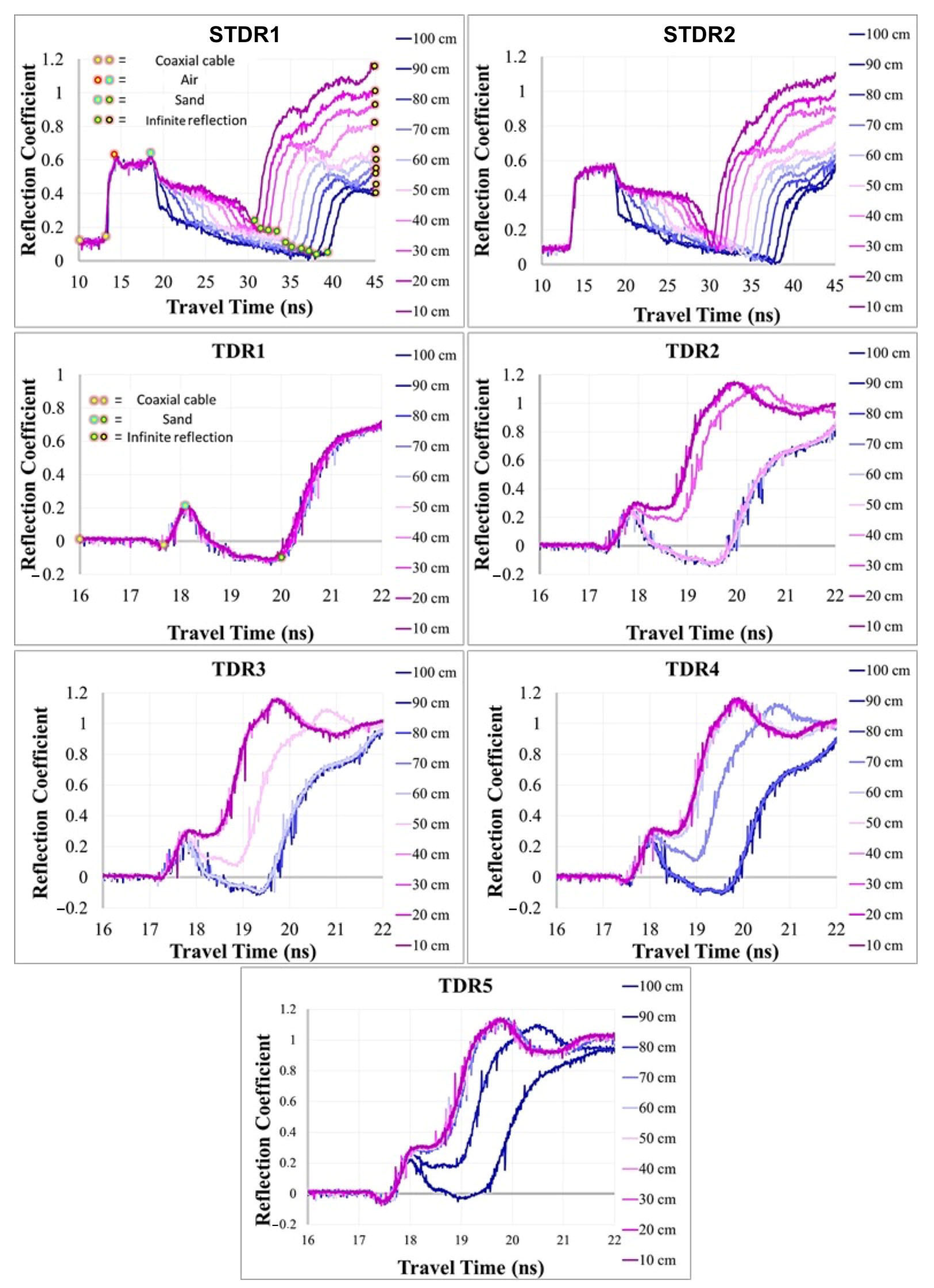
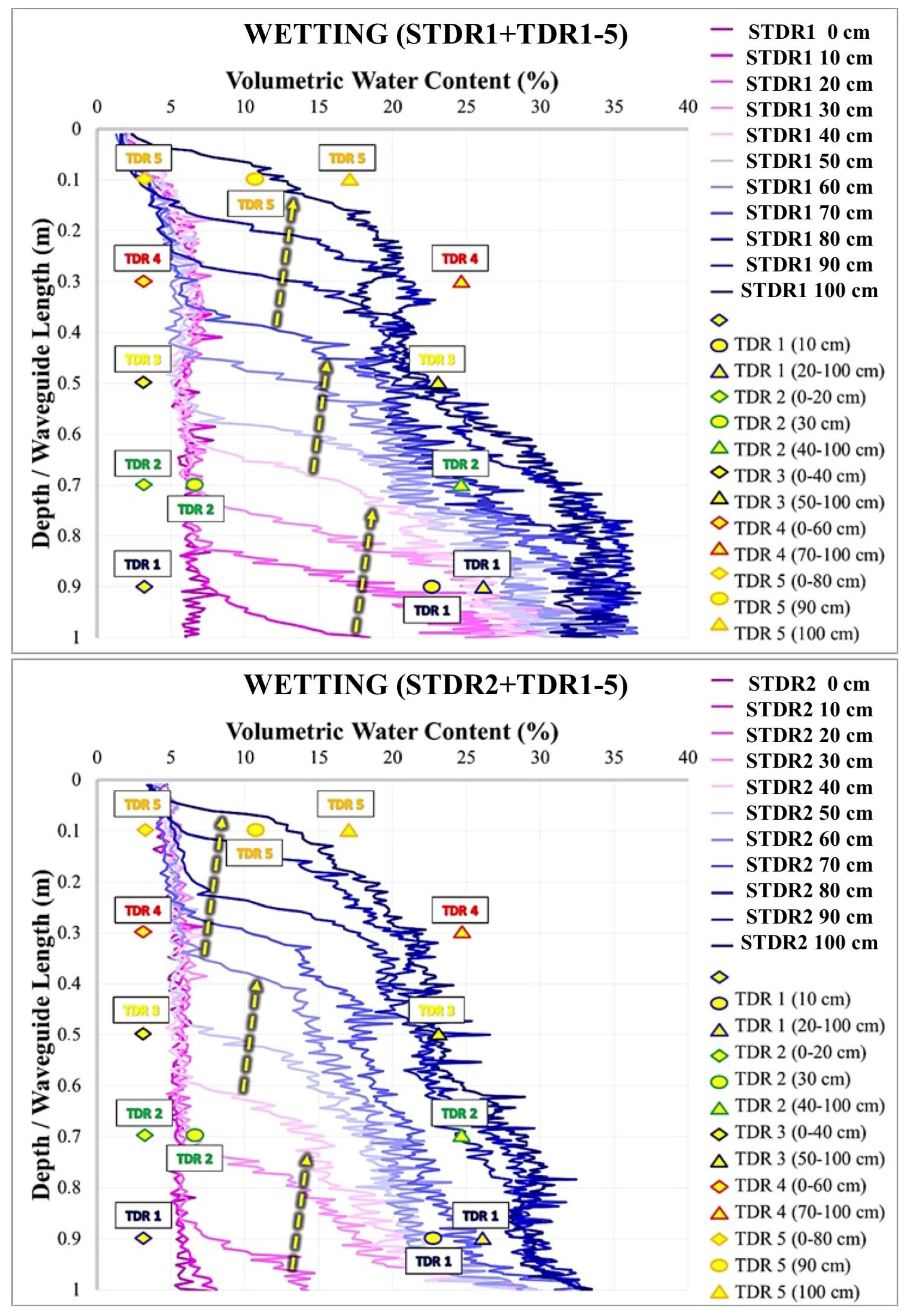
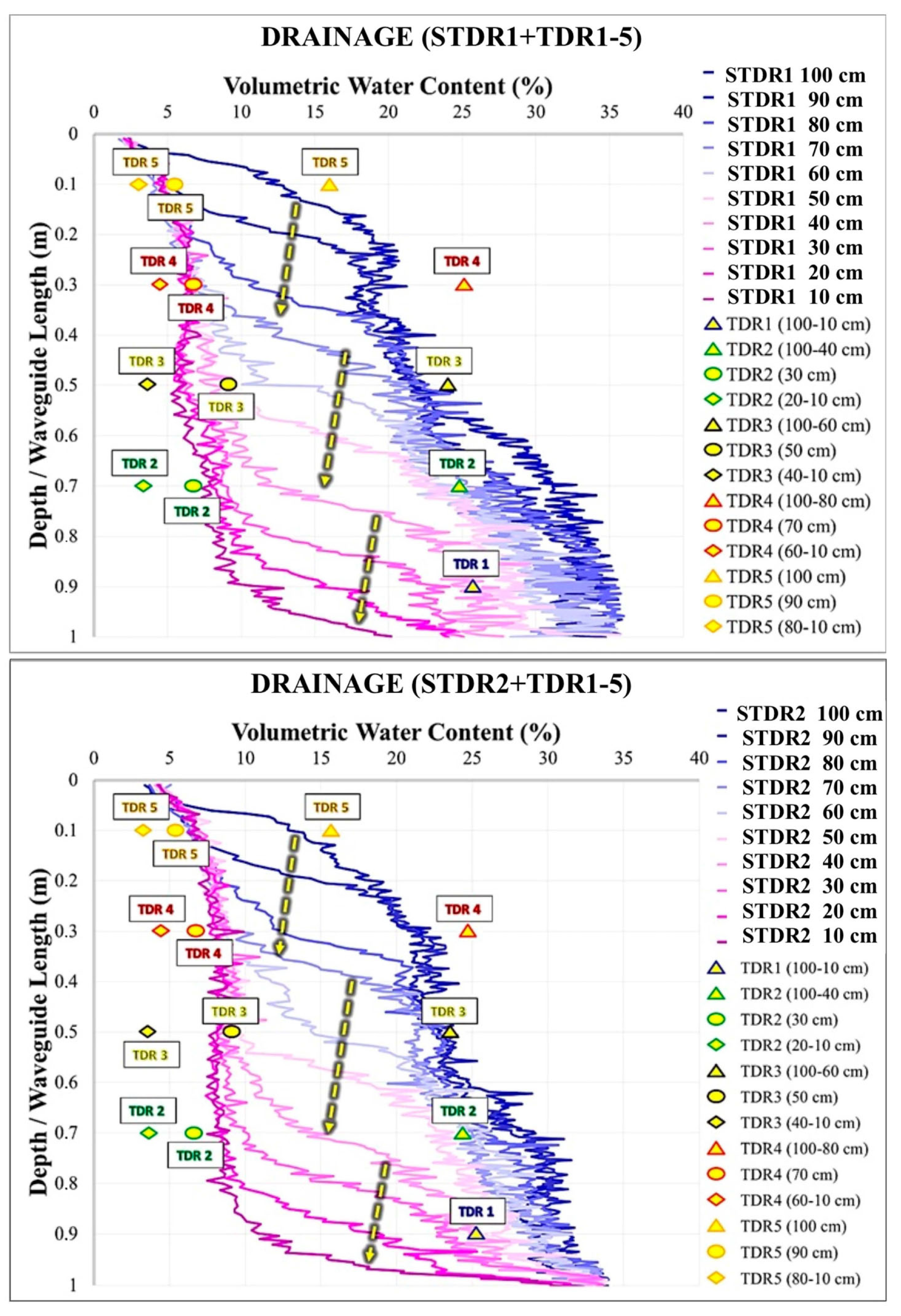
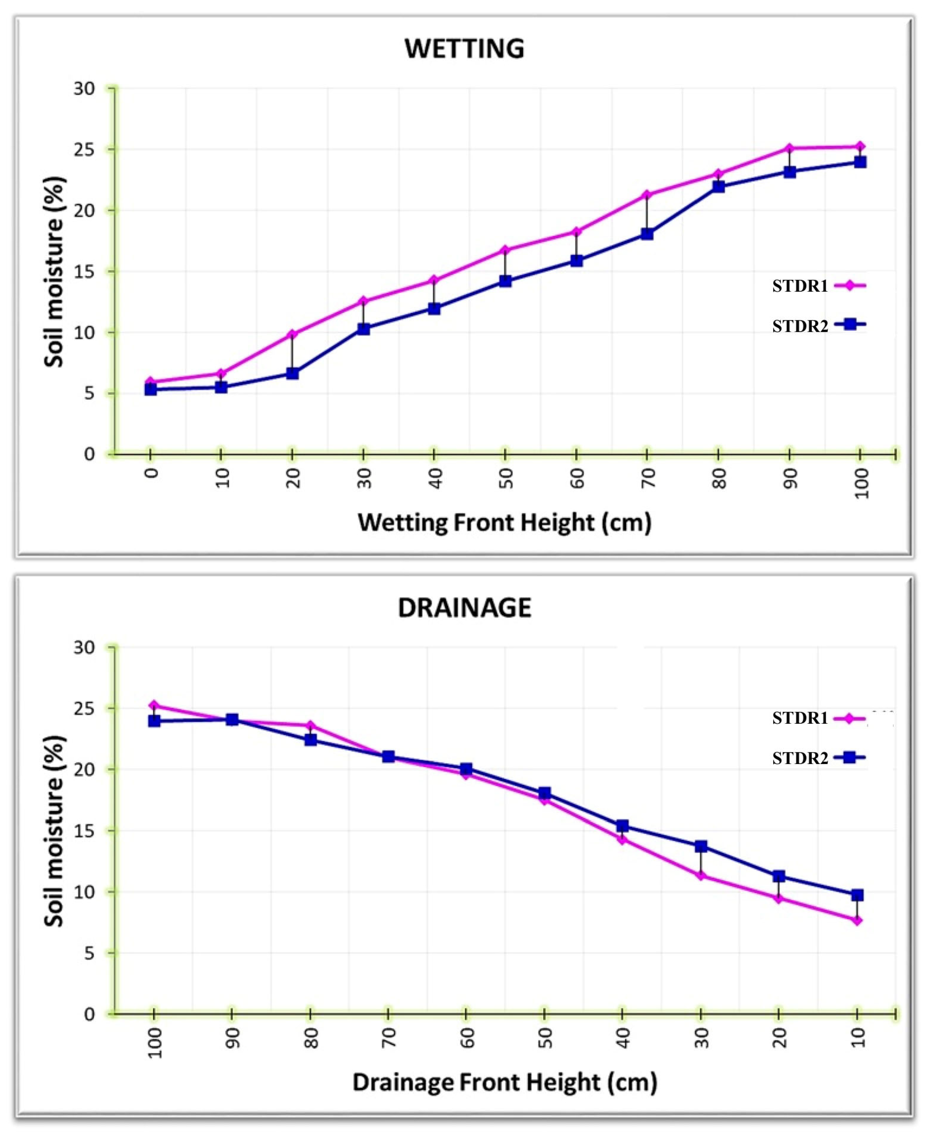
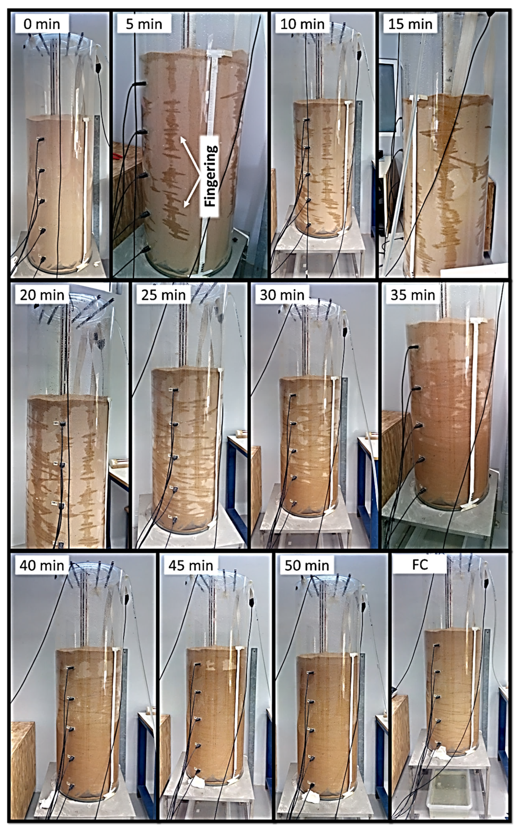
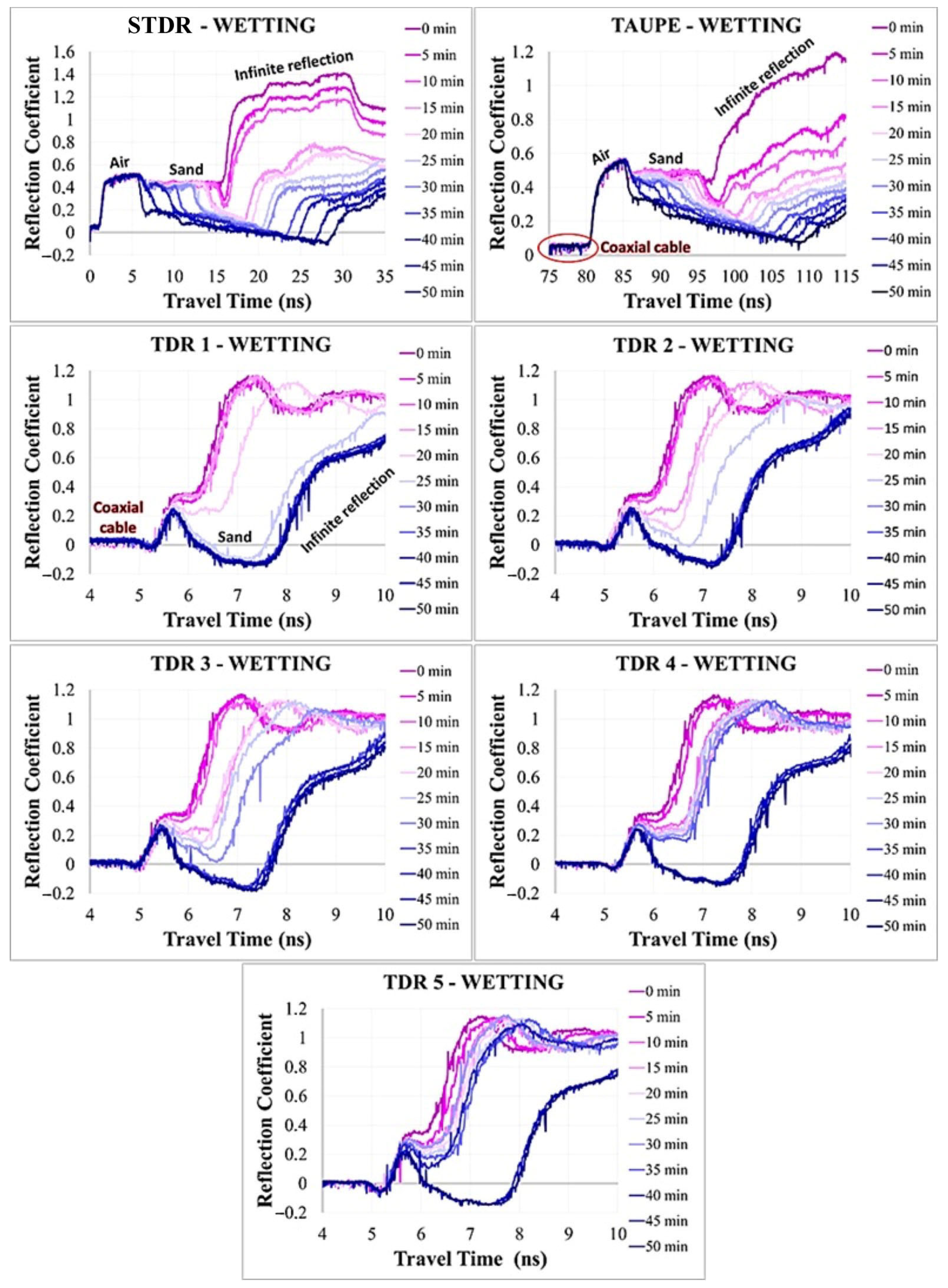
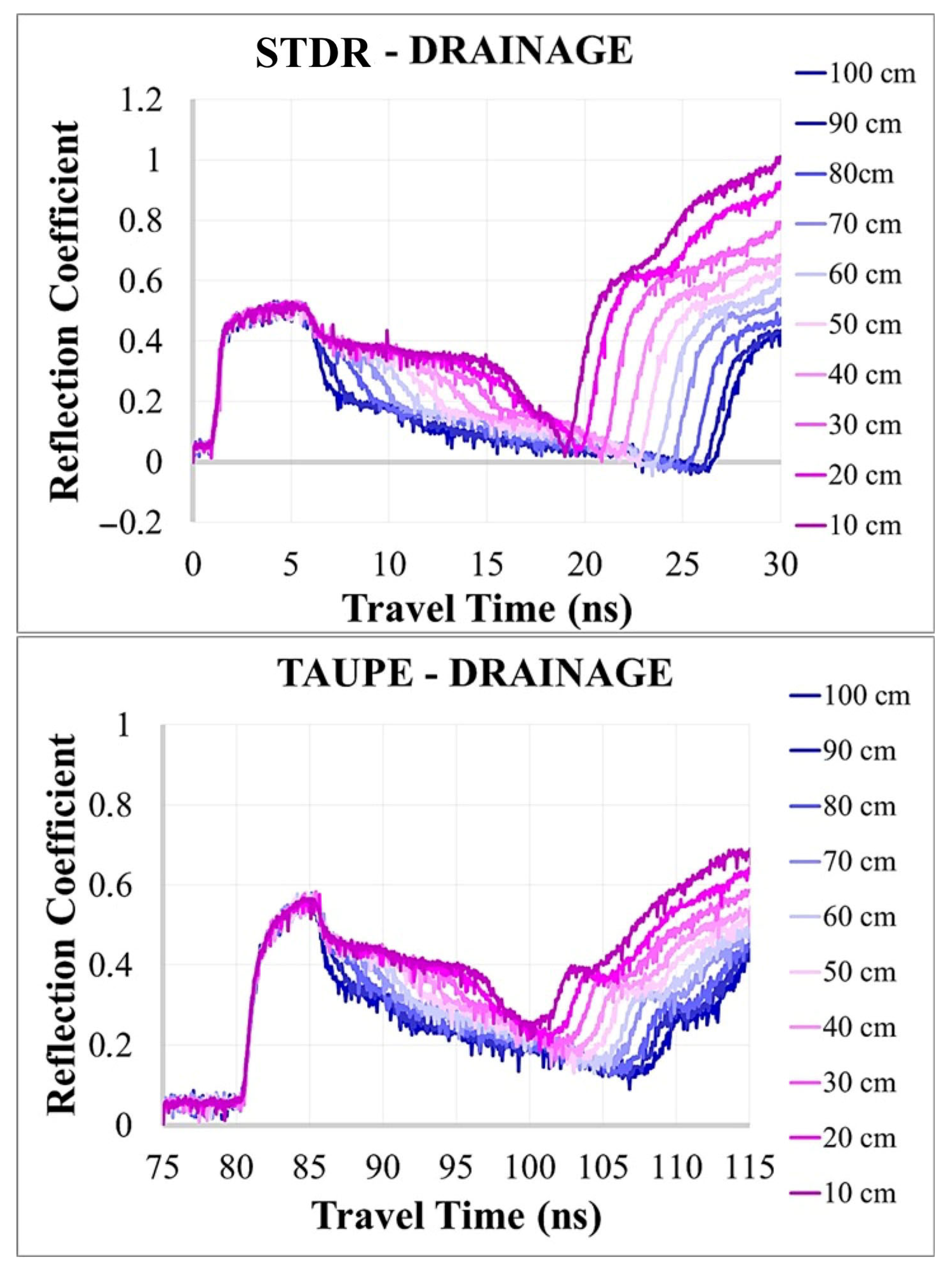
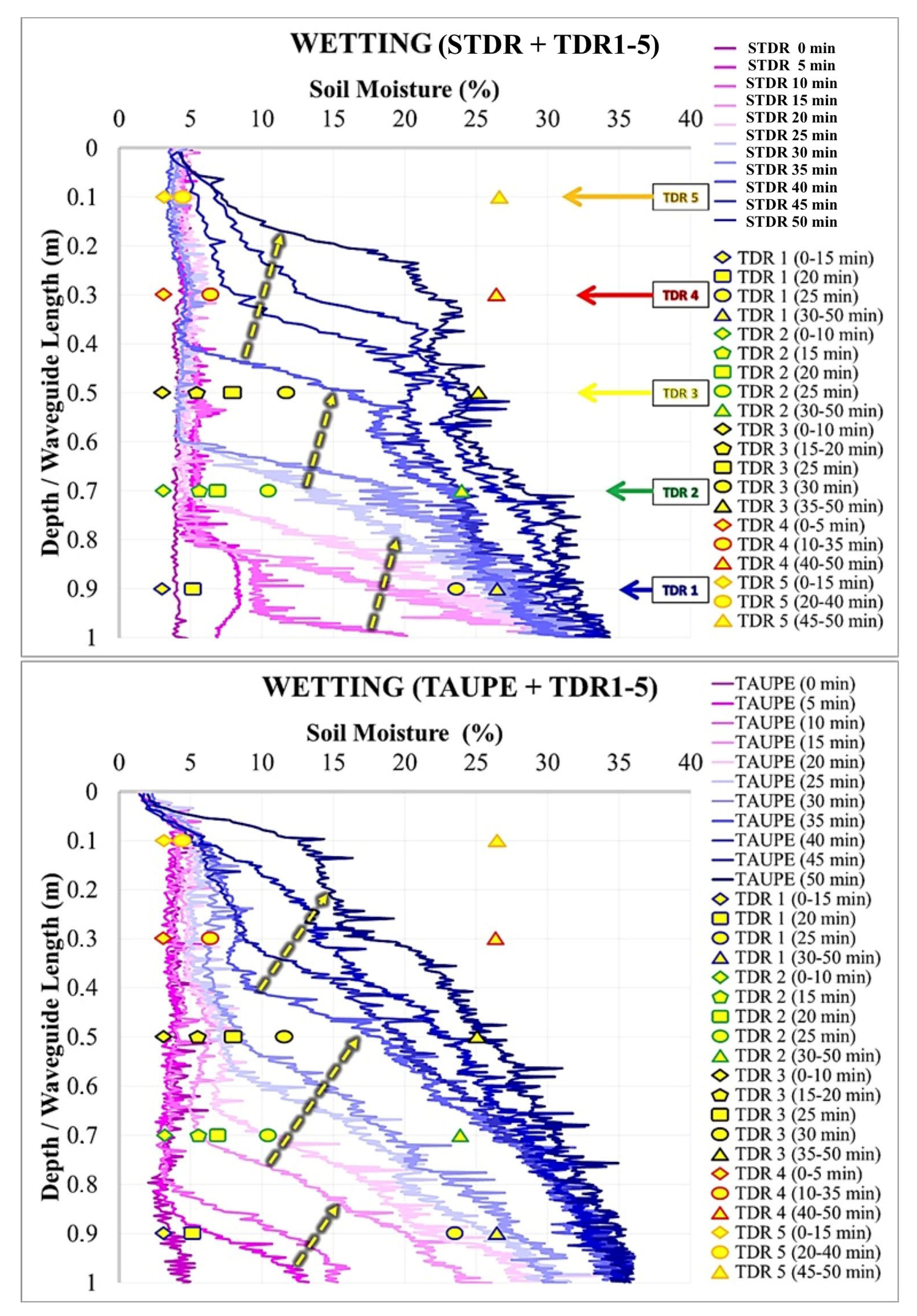
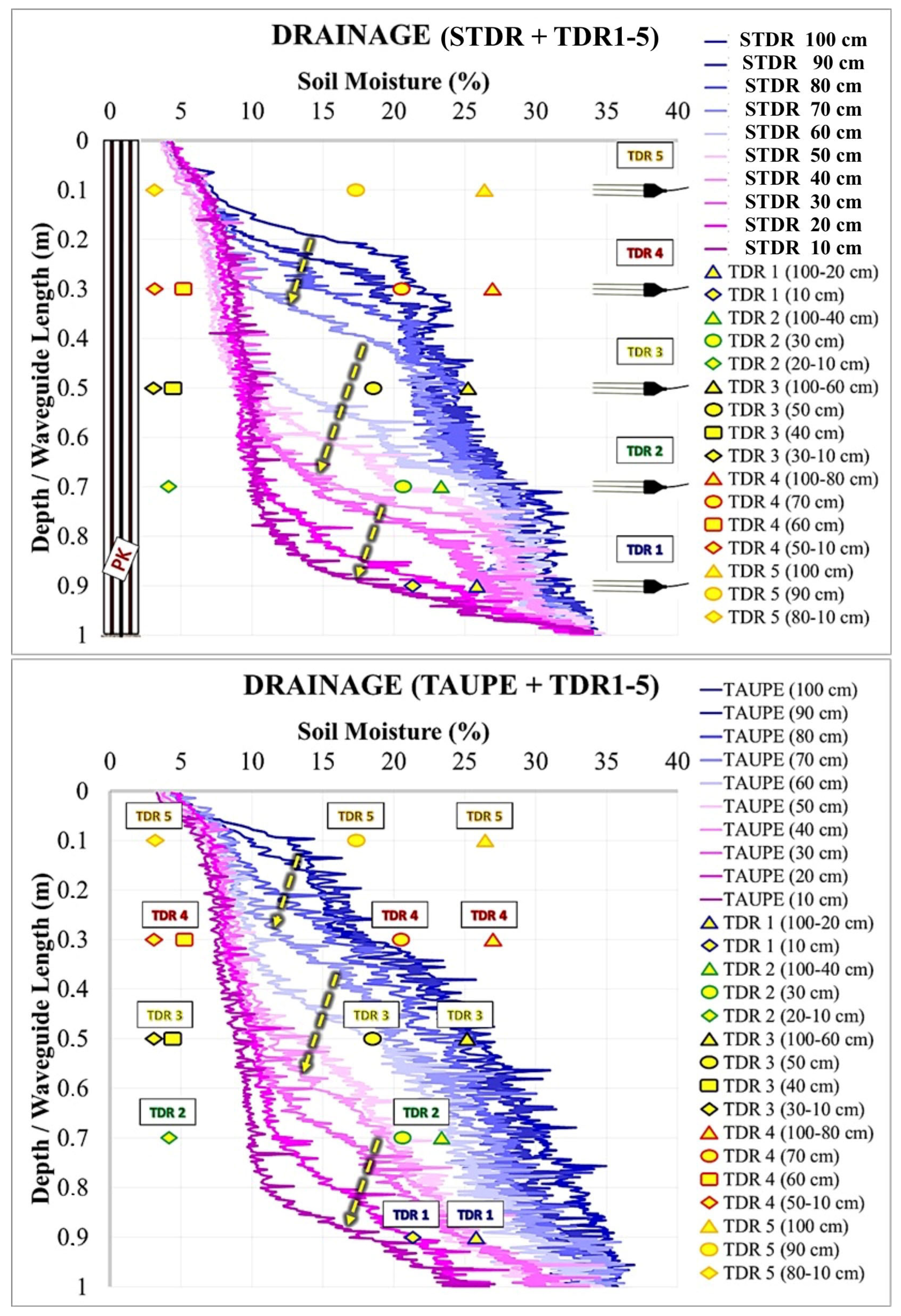
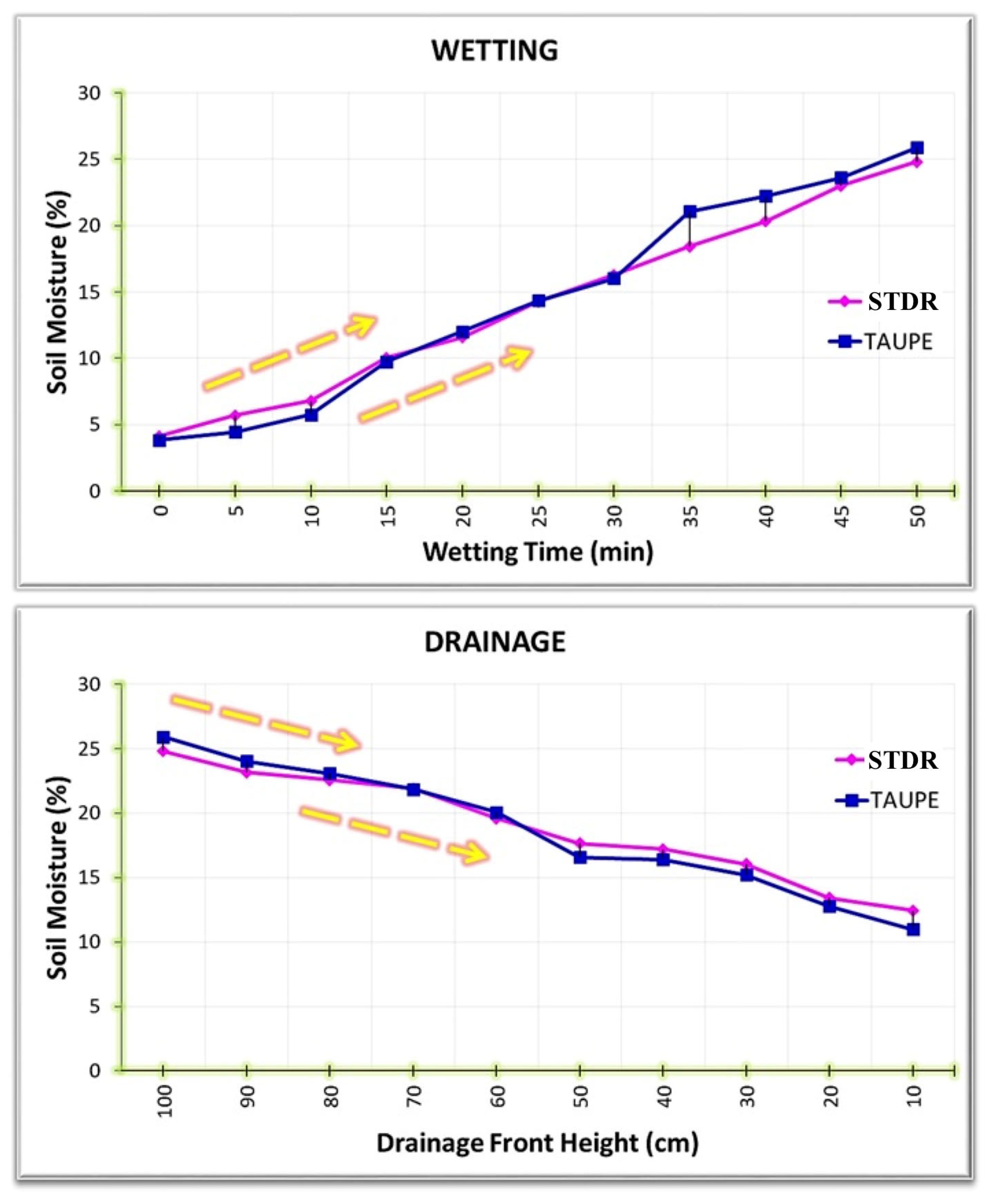
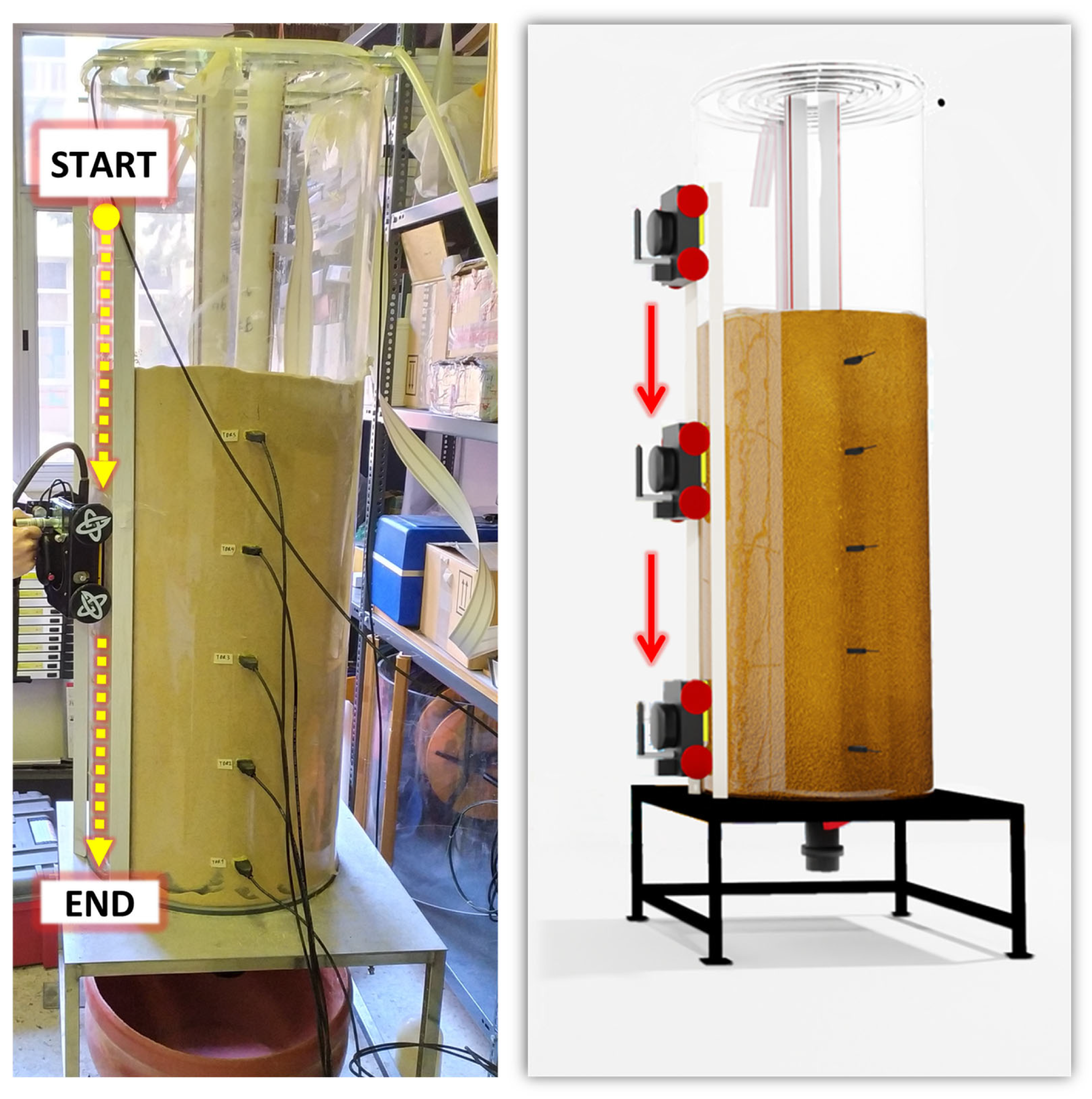
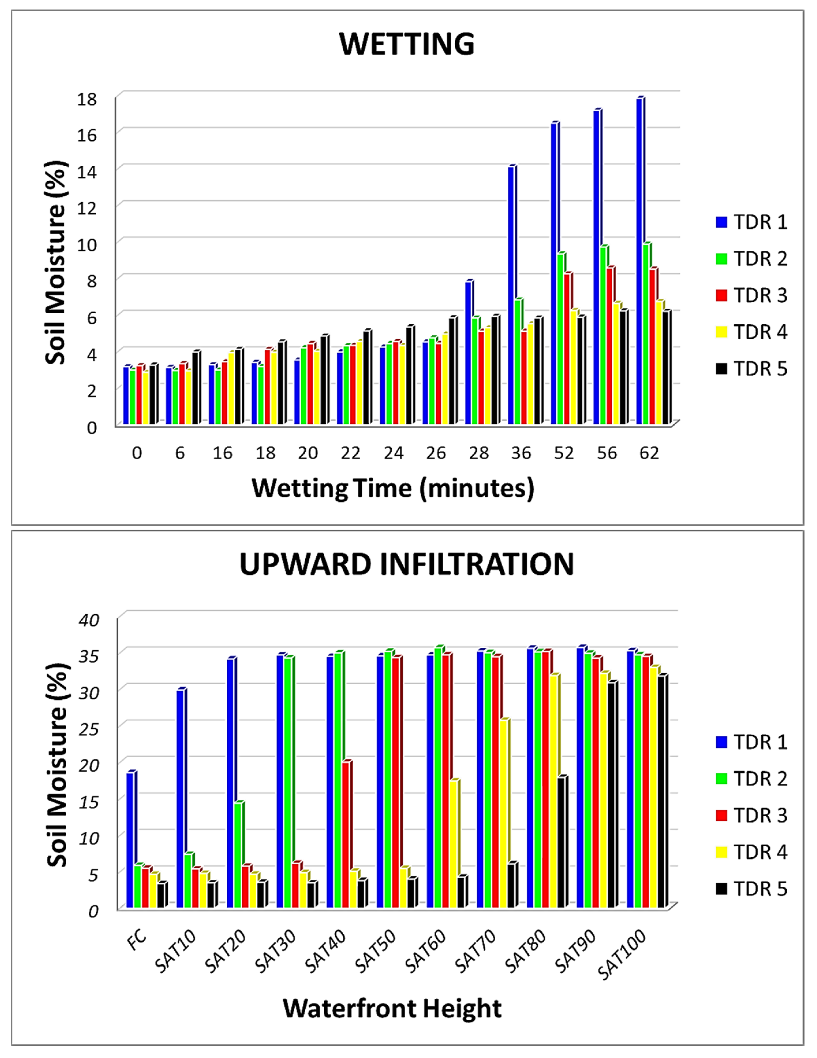
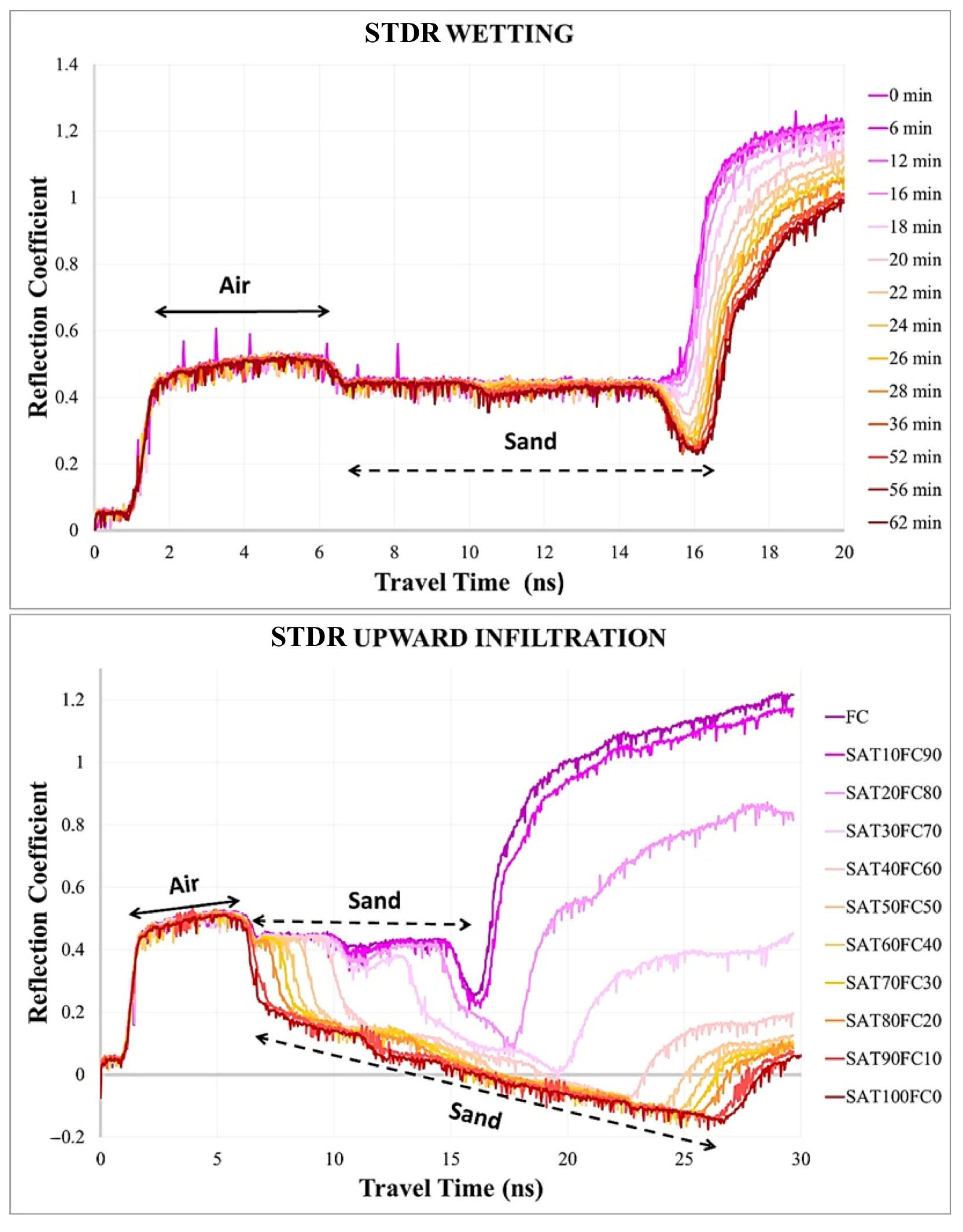
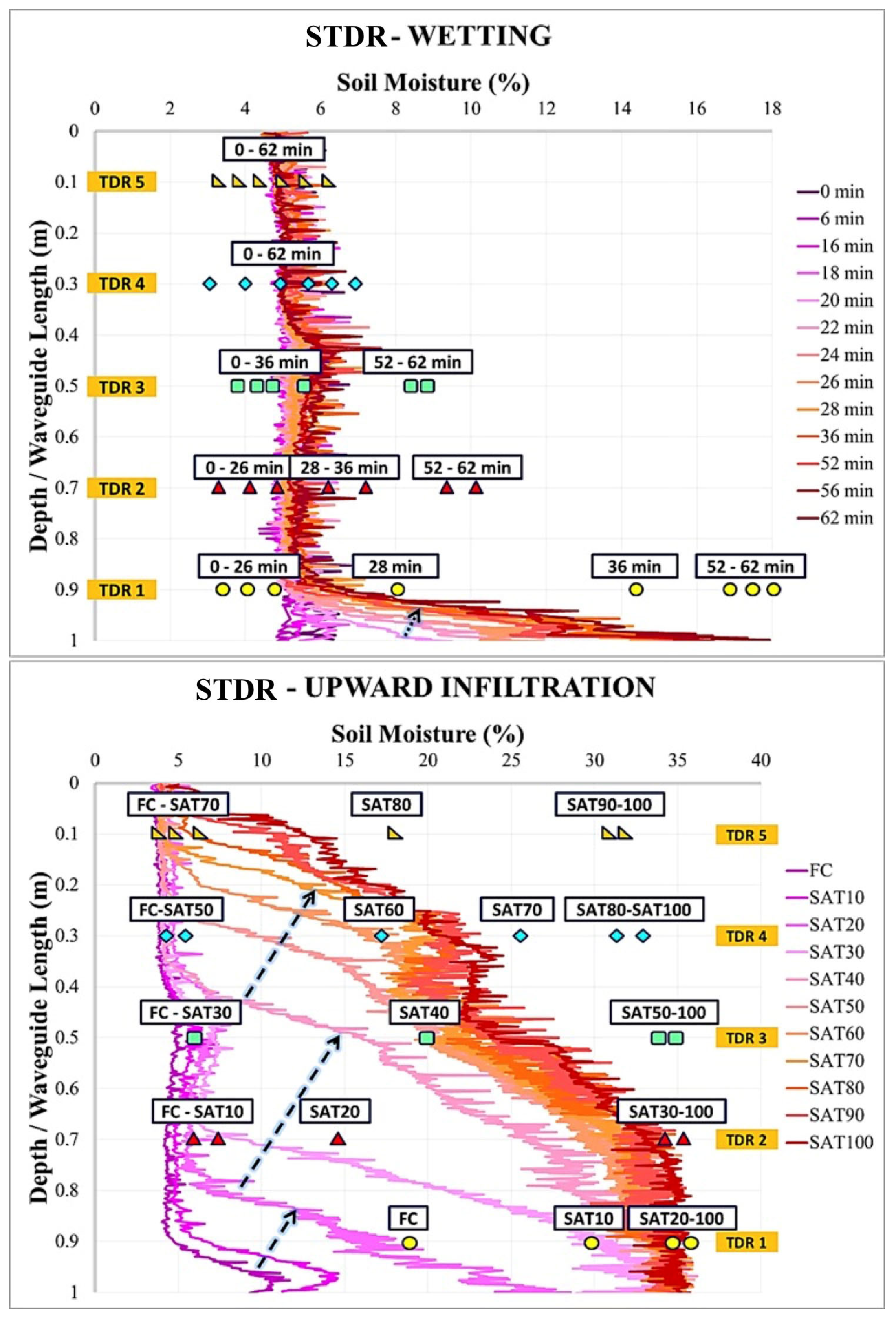

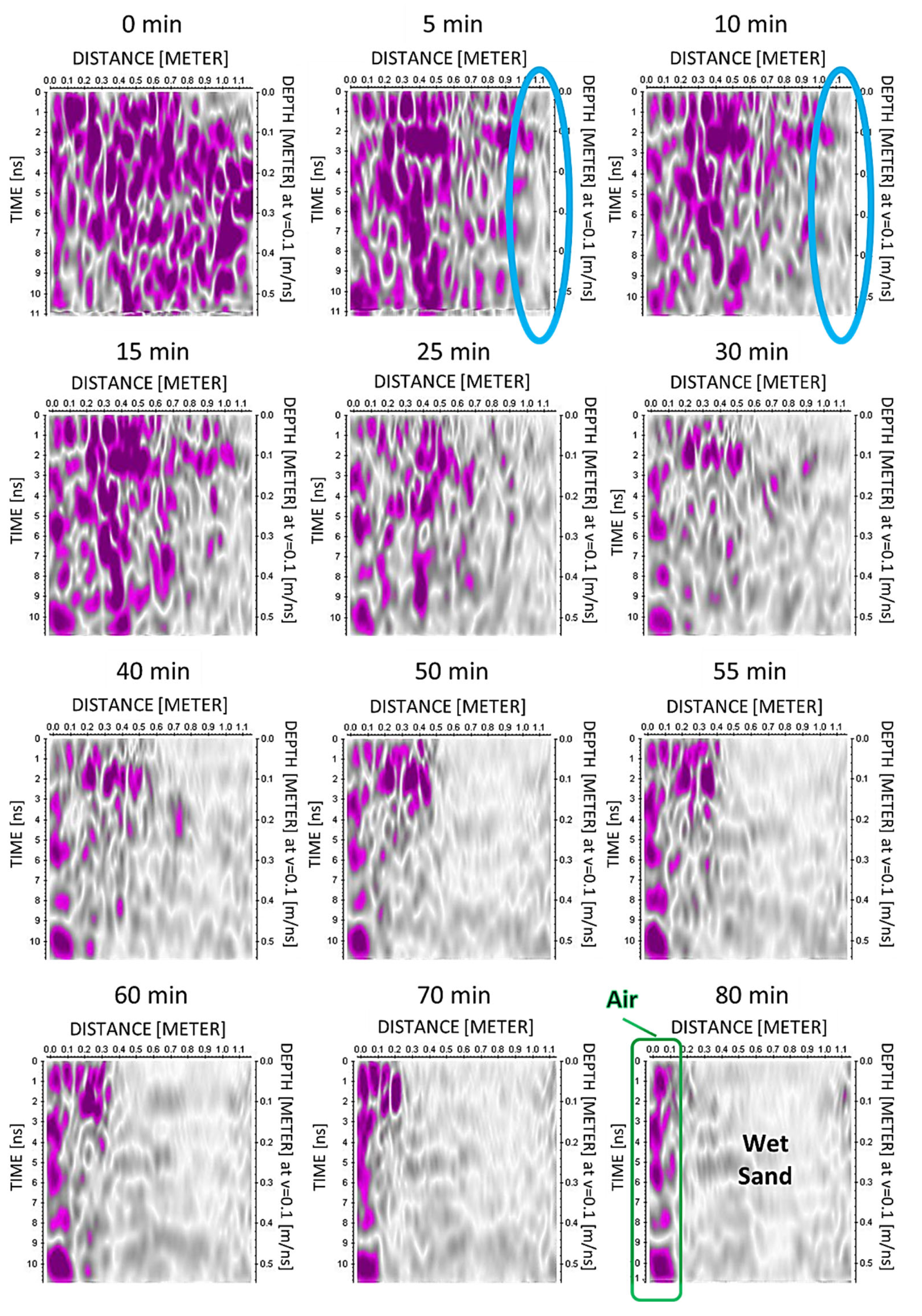
Disclaimer/Publisher’s Note: The statements, opinions and data contained in all publications are solely those of the individual author(s) and contributor(s) and not of MDPI and/or the editor(s). MDPI and/or the editor(s) disclaim responsibility for any injury to people or property resulting from any ideas, methods, instructions or products referred to in the content. |
© 2025 by the authors. Licensee MDPI, Basel, Switzerland. This article is an open access article distributed under the terms and conditions of the Creative Commons Attribution (CC BY) license (https://creativecommons.org/licenses/by/4.0/).