Article

Optimizing Ecological Water Replenishment in Xianghai Wetlands Using CNN-LSTM and PSO Algorithm Under Secondary Salinization Constraints

1
Key Laboratory of Groundwater Resources and Environment, Jilin University, Ministry of Education, Changchun 130021, China
2
Jilin Provincial Key Laboratory of Water Resources and Environment, Jilin University, Changchun 130021, China
3
College of New Energy and Environment, Jilin University, Changchun 130021, China
*
Author to whom correspondence should be addressed.
Water 2025, 17(13), 1886; https://doi.org/10.3390/w17131886
Submission received: 4 April 2025 / Revised: 17 June 2025 / Accepted: 18 June 2025 / Published: 25 June 2025

Abstract

Wetlands play a crucial role in water purification, climate regulation, and biodiversity conservation. However, the Xianghai wetlands (situated in Tongyu County, Jilin Province, China) have experienced severe ecological degradation due to natural factors and unsustainable human activities, leading to declining groundwater levels and intensified salinity issues. To address these problems, this study aims to optimize ecological water replenishment strategies for the Xianghai nature reserve by integrating groundwater numerical simulation, surrogate modeling (convolutional neural network–long short-term memory neural network, CNN-LSTM), and intelligent optimization algorithms (Particle Swarm Optimization, PSO). During the design of the water replenishment scheme, the objective function maximizes the replenishment volume while considering the secondary salinization of soil in the reserve and its surrounding areas as a constraint. The results show that the surrogate model established using the convolutional neural network–long short-term memory neural network achieved high accuracy, with R2 values of 0.9996 and 0.9962 and MREs of 0.0023 and 0.0089 for training and validation sets, respectively; Compared to the random replenishment scheme, the optimized water replenishment scheme significantly reduces secondary salinization. After 10 years water replenishment, the optimized scheme exhibited a 2 km2 reduction in the salinized area compared to the randomized scheme, with the degree of salinization being reduced from moderate to mild. This method improves ecological sustainability and can be adapted to meet local water use demands. This simulation-optimization method provides an effective approach for designing water replenishment schemes that address secondary salinization.

1. Introduction

Wetlands are one of the most important ecosystems on Earth, playing irreplaceable roles in water purification, climate regulation, and the protection of biodiversity [1,2]. In recent years, influenced by natural processes and irrational human exploitation of water and soil resources, the water resources upon which the wetlands of Xianghai depend have diminished, leading to severe degradation. It is urgent to enhance the protection of the Xianghai wetlands [3,4,5,6,7]. As wetland environmental protection methods rapidly evolve, ecological water replenishment has increasingly become one of the main ecological restoration strategies used to prevent wetland degradation and promote ecological succession in wetlands [8]. However, artificial water replenishment in wetlands inevitably leads to salinization. The groundwater level rises with artificial replenishment. Under intense evaporation, the elevated groundwater level increases the salinity of the soil surface, creating conditions for secondary salinization [9,10]. Therefore, to minimize the adverse effects of wetland replenishment on the surrounding environment, it is essential to simulate the replenishment to predict its impact on the environment, design ecological replenishment schemes, and select the optimal replenishment strategy, which is an indispensable part of the entire replenishment process.
Optimization methods represent a quintessential approach in the study of optimized design for water replenishment schemes [11]. Yakowitz [12] applied optimization methods to the problem of wetland water resource management. Since then, numerous researchers have expanded and improved optimization models and algorithms, applying them to various wetland water replenishment issues [13,14,15,16,17]. Some studies have considered economic factors, aiming to minimize the cost of water replenishment, balance economic benefits with water resource availability, or maximize economic returns [18,19,20]; others have focused on ecological and environmental issues, optimizing water replenishment schemes to protect habitats for flora and fauna, enhance environmental quality, or improve water quality [21,22,23]. In areas with shallow water tables and high evaporation rates, the replenishment process can lead to salinization issues. Such conditions are prevalent in the Xianghai nature reserve, where high evaporation and shallow groundwater levels facilitate salinization. In designing water replenishment schemes for this area, it is essential to consider and mitigate salinization. Existing studies on water replenishment for the Xianghai reserve primarily focus on the required water volume and its impact on flora and fauna [24,25], without addressing salinization. However, there is a significant scientific gap in the current research: most previous studies have not considered soil secondary salinization as a key constraint in water replenishment optimization, especially in regions with both shallow groundwater tables and high evaporation rates. Furthermore, integrated frameworks that combine advanced data-driven surrogate models with intelligent optimization algorithms for ecological water management in saline-prone wetlands remain scarce. Addressing this gap is essential for developing sustainable water replenishment strategies in sensitive wetland ecosystems. Therefore, this study aims to optimize the water replenishment scheme for the Xianghai nature reserve by considering the issue of soil secondary salinization.
This study focuses on the Xianghai nature reserve and investigates the optimization of water replenishment schemes through the combined use of groundwater numerical simulation, data-driven surrogate models, and intelligent optimization algorithms. During the design of the water replenishment scheme, the objective function maximizes the replenishment volume while considering the secondary salinization of soil in the reserve and its surrounding areas as a constraint
The optimization process necessitates tens of thousands of invocations of the numerical model, resulting in a substantial computational load. Surrogate models, capable of approximating the input–output relationship of the simulation model with significantly less computational effort, offer a solution to this challenge [26,27,28,29,30,31]. By directly utilizing surrogate models, the computational burden and time associated with repeatedly invoking the simulation model during the optimization process can be markedly reduced. Traditional surrogate model construction methods, such as Kriging, Support Vector Machines (SVMs), and Back-Propagation (BP) Neural Networks, are categorized under shallow machine learning. These models demonstrate good fitting performance on simple problems. However, their accuracy in capturing the nonlinear mapping relationships inherent in simulation models under complex conditions needs further improvement. For example, Kriging and SVMs are limited in representing highly nonlinear relationships when groundwater flow and salinity dynamics interact under changing climatic and anthropogenic conditions. Conventional neural networks, while useful for simple regression, often fail to model the complex temporal and spatial variabilities in wetland hydrology. As a result, more powerful modeling tools are needed to overcome these limitations. CNN-LSTM neural network is an amalgamation of two distinct neural network models, the convolutional neural network (CNN) and long short-term memory (LSTM). The convolution and pooling operations unique to CNNs efficiently extract features from data, while LSTM networks exhibit robust memory capabilities, being especially effective in processing sequential data. Leveraging the strengths of these two neural network models, their combination offers potent feature extraction and time-series prediction capabilities. To date, there has been no reported application of CNN-LSTM neural networks in establishing surrogate models for groundwater numerical simulation. Thus, this study is the first to employ CNN-LSTM surrogate models in the context of groundwater replenishment optimization, specifically addressing secondary soil salinization. This innovative integration is expected to significantly improve surrogate modeling accuracy for complex multi-dimensional hydrological systems while also reducing the computational burden during optimization. This presents an urgent need for empirical validation. Therefore, this study employs the CNN-LSTM neural network to establish a surrogate model, investigating its fitting performance under multi-dimensional input and output scenarios. To comprehensively evaluate the performance and advantages of the proposed CNN-LSTM surrogate model, a Kriging surrogate model is also constructed for comparative analysis, enabling a more systematic comparison of the fitting accuracy and generalization ability of different surrogate modeling approaches in groundwater contamination monitoring applications.
Fitting in this context, the main objective of this study focuses on the Xianghai nature reserve as a case study area, considering the problem of secondary soil salinization. Based on simulation–optimization methods, an optimization model has been established with the total amount of water replenishment as the objective function and the monthly water replenishment volumes as decision variables. Ecological water demand, available water supply, and the observed post-replenishment water table depths serve as constraints to prevent secondary salinization. To reduce the computational load during the solution process, surrogate models of the simulation model were constructed using both a CNN-LSTM neural network and the traditional Kriging approach. By comparing the performances of these surrogate models, the CNN-LSTM was selected and embedded into the optimization model as an equality constraint due to its superior fitting accuracy. Ultimately, the Particle Swarm Optimization (PSO) algorithm was employed to solve the optimization model, yielding a water replenishment scheme that meets the requirements. This provides a scientific basis for ecological water replenishment in the Xianghai nature reserve.
In summary, this research pioneers a simulation–optimization framework that integrates CNN-LSTM-based surrogate modeling with PSO, specifically targeting groundwater replenishment in wetlands under salinization constraints. The proposed method not only advances computational efficiency but also provides a robust decision-making tool for ecological water management in regions with similar hydrological and environmental challenges. This provides a scientific basis for ecological water replenishment in the Xianghai nature reserve.

2. Materials and Methods

2.1. Framework for Optimization Design of Replenishment Scheme Based on CNN-LSTM and PSO Algorithm

The optimization design framework for water replenishment schemes consists of three main components: the numerical simulation model, the surrogate model, and the water replenishment scheme optimization design. The framework for designing the water replenishment scheme is illustrated in Figure 1.
(1)
Based on natural geography, geology, and hydrogeological conditions, a hydrogeological conceptual model was established. Subsequently, a mathematical model was developed and solved using MODFLOW. This model was then subjected to identification and validation.
(2)
Latin hypercube sampling was utilized to sample the input variables, which are then fed into the simulation model to acquire the output samples. A surrogate model for the simulation model was constructed using a CNN-LSTM neural network, employing input–output samples to train the deep learning neural network.
(3)
An optimization model was established with the total monthly replenishment volume as the decision variable and the maximum total replenishment volume of the replenishment area as the objective function. The surrogate model was embedded as an equation constraint within the optimization model, and the PSO optimization algorithm is used to solve the optimization model.

2.2. Latin Hypercube Sampling Method

Latin hypercube sampling (LHS) was proposed by scholars McKay et al. [32] as a stratified sampling method for approximating random sampling from multivariate parameter distributions. This method has been extensively utilized for acquiring datasets for surrogate models [33]. The basic steps of LHS sampling are as follows:
(1)
First, define the number of sampling variables m   and the required sample size n . Then, meticulously divide the feasible range of each variable x 1 , x 2 , , x m into n non-overlapping intervals.
(2)
Draw one sample from each interval for the variables x 1 , x 2 , , x m , so that for any given variable x i , n samples are obtained.
(3)
Combine the n samples of variable x 1 with the n samples of variable x 2 to obtain n 2 sample combinations; then, combine these with the n samples corresponding to variable x 3 to get n 3 sample combinations. Perform combinations in the same manner for the samples of each variable to ultimately obtain n m different sample combinations.
(4)
From the n intervals of the m -dimensional vectors obtained in step 3, one element was randomly selected from each interval to form a sample; and the same method was ultimately used to obtain n samples, which are the results of the sampling.

2.3. CNN-LSTM Neural Network

CNN-LSTM neural network is created by combining two neural network models, the CNN and LSTM, which boasts significant advantages in processing image and textual information. It possesses powerful feature extraction capabilities and time-series prediction abilities, effectively extracting and utilizing data characteristics, thus enhancing the model’s predictive accuracy. It has excelled in various fields, including visual computing, language intelligence, and speech technology, for tasks such as image captioning, text sentiment analysis, and speech transcription [34,35]. The architecture is ingeniously designed and primarily includes input import and multi-layer interaction: First, the information flows through the convolutional units of the CNN, capturing deep-level features of the data through dynamic filters. Next, it undergoes refinement in the max-pooling layer, which retains critical information while effectively compressing the data dimensions. During this process, the Dropout layer plays a crucial role by randomly “turning off” some neurons, strategically reducing the network’s complexity, lowering the risk of overfitting, and enhancing the model’s generalization ability (Figure 2). In summary, this process can be outlined as follows:
(1)
Data enter the CNN convolutional layer, where wide convolutional kernels adaptively extract features.
(2)
Subsequently, features are refined and optimized through the max-pooling layer, balancing information retention and resource saving. The Dropout layer acts as a regularization method, enhancing the model’s robustness.
(3)
The dimensionally reduced feature data are then input into the LSTM layer as features, which trains the neural network and autonomously learns sequence features.
(4)
The fully connected layer integrates the features extracted by previous layers, providing a basis for the final output results.
(5)
The output data are produced, completing the task.
In the CNN-LSTM neural network, the CNN primarily deals with spatial data such as images or texts, extracting features from the input data through convolutional operations and pooling. These features are then processed by the LSTM layer to capture long-term dependencies within time-series data. Finally, the fully connected layer integrates these features to form the basis for the final output. This combination allows the CNN-LSTM neural network to possess both the CNN’s feature extraction capabilities and LSTM’s time-series prediction abilities.
Figure 2. CNN-LSTM neural network structure diagram.
Water 17 01886 g002

2.4. Optimization Model for Water Replenishment Scheme Design

The objective function for the optimization process is defined as the maximization of the total ecological water replenishment volume over the entire water replenishment period:
m a x Z = j = 1 N z t = 1 N m Q j , t
where Z is the total replenishment volume; Q j , t is the water replenishment volume in zone j and month t ; N z is the number of replenishment zones; and N m   is the number of replenishment months.
The above objective function is subject to the following constraints:
(1)
Ecological water demand constraints
Q j , t Q j , t m i n
where Q j , t m i n is the ecological water demand;
(2)
Water supply constraints
j = 1 N z Q j , t Q j , t m a x
where Q j t m a x is available water supply;
(3)
Water level depth constraint considering the problem of secondary soil salinization
d i , 10 d i , m i n
where d i , 10 is the water level burial depth of observation point i after 10 years, and d i , m i n is the minimum water level burial depth of observation point i ;
(4)
Equality constraints constituted by the surrogate model
d i , 10 = M ( Q j , t )
where d i , 10 is a function of the replenishment volume, representing the simulated water table depth at observation point i after 10 years, which is predicted by the established surrogate model M derived from numerical simulation model.

2.5. Particle Swarm Optimization Algorithm

In this study, the Particle Swarm Optimization algorithm was selected as the optimization method due to its well-documented advantages over other evolutionary algorithms such as the Genetic Algorithm (GA) and Differential Evolution (DE). Compared to the GA, PSO is easier to implement, requires fewer control parameters, and typically converges faster because it does not involve complex operations such as crossover and mutation [36]. Furthermore, previous studies have shown that PSO has been demonstrated to be robust and efficient in solving high-dimensional and nonlinear optimization problems encountered in water resource management [37,38]. Therefore, PSO was chosen in this study as a suitable and efficient optimizer for the simulation–optimization framework.
Particle Swarm Optimization (PSO), inspired by the collaborative strategies of bird flocks in nature [39], is an innovative optimization technique that draws on the wisdom of biological foraging behavior to find solutions. Within this framework, each potential solution to the optimization problem is viewed as a virtual bird, or a dynamic particle, in the search domain. These particles explore the solution space through their own velocity and direction, with fitness values assigned to each particle to guide them towards the optimal state.
In this D-dimensional exploration stage, each particle’s state includes its current position X i , current flying speed V i , and the best experienced position P i (the position with the best fitness value) of particle i and are represented as:
X i = ( x i 1 , x i 2 , , x i D ) V i = ( v i 1 , v i 2 , , v i D ) P i = ( p i 1 , p i 2 , , p i D )
For a maximization problem, where the objective f ( x ) is to maximize a function, the update rule for a particle’s personal best position is as follows:
P i t + 1 = P i t   f ( X i t + 1 ) f ( P i t ) X i t + 1   f ( X i t + 1 ) < f ( P i t )
where P i t represents the best position experienced by particle i at time t ; X i t + 1 is current position of particle i at time t + 1 ; and P i t + 1 denotes the best position experienced by particle i at time t + 1 .
Suppose the number of particles in the group is S , and the best position experienced by all particles in the group is P g t , which is called the global best position, that is:
f P g ( t ) = max { f P 1 t , f P 2 t , , f P s t } , P g t P 1 t , P 2 t , , P 3 ( t )
The evolution equation of particle i can be described as:
v i j t + 1 = v i j t + C 1 r 1 P i j t x i j t + C 2 r 2 t [ P g j t x i j t ]
x i j t + 1 = x i j t + v i j ( t + 1 )
where the subscript j represents the j-th dimension of the particle, the subscript i represents the i-th particle, and v i j t denotes the velocity of the i-th particle in the j-th dimension at the t-th generation; C 1 and C 2 are both acceleration constants (learning factors); r 1 , r 2 are two mutually independent random numbers; and P g t are the positions of the global optimal particles. It can be seen from the above equation that C 1 , C 2 combining particle learning from individuals and learning from groups enables particles to learn from the search experience of the body itself [the second term on the right side of Equation (9)] and the search experience of the group [the third term on the right side of Equation (9)] for dynamic adjustment.
Adding inertia weight ω to the term v i j t in Equation (9) is the Particle Swarm Optimization algorithm with the inertia factor:
v i j t + 1 = ω v i j t + C 1 r 1 P i j t x i j t + C 2 r 2 t [ P g j t x i j t ]
As the ω value increases, the Particle Swarm Optimization (PSO) algorithm’s ability for global exploration strengthens, but its capacity to refine local optima weakens. Conversely, when the ω value is lower, the global vision may diminish, but the algorithm becomes more adept at precisely searching local optima. One strategy is to employ a dynamically adjusted ω value, which can significantly enhance optimization performance compared to a fixed value, better adapting to the complexities of the search process. Generally, the linearly decreasing weight (LDW) strategy is used [40]:
ω ( t ) = ω i n i ω e n d G k g G k + ω e n d
where G k is the maximum number of iterations; g is the current number of iterations; ω i n i is the initial inertia weight; and ω e n d is the inertia weight when iterating to the maximum evolutionary algebra, and these generally take typical weights: ω i n i = 0.9 and ω e n d = 0.4.
This dynamic adjustment strategy for the momentum weight (ω) significantly enhances the overall efficiency of the Particle Swarm Optimization (PSO) algorithm. It cleverly balances the flexibility between global exploration and local refinement during the search tasks.

2.6. GMS Software and MODFLOW Model

The groundwater flow simulation in this study was performed using the MODFLOW model (developed by the U.S. Geological Survey), integrated within the Groundwater Modeling System 10.6.6 (GMS, Aquaveo, LLC, Provo, UT, USA) software environment. MODFLOW is a widely used, modular finite-difference groundwater flow model that supports the simulation of groundwater movement under a variety of hydrogeological conditions. Its flexible structure allows for the definition of complex boundary conditions, aquifer properties, and various hydrological processes.
GMS is a comprehensive modeling platform that provides a user-friendly graphical interface for groundwater model construction, parameter assignment, numerical solution, and result visualization. It facilitates the pre-processing of spatial data, the establishment and editing of model grids, the assignment of hydraulic parameters, the configuration of boundary conditions, and the coupling of different simulation modules. GMS also supports post-processing functionalities, such as the visualization of simulated groundwater heads, flow vectors, and water budgets. The main advantages of using MODFLOW within GMS include its robustness, flexibility, and extensive validation in a wide range of practical groundwater applications.
All hydrogeological and meteorological data used in the simulations, including precipitation, evaporation, soil properties, and groundwater levels, were obtained from field surveys and site documentation.

3. Case Application

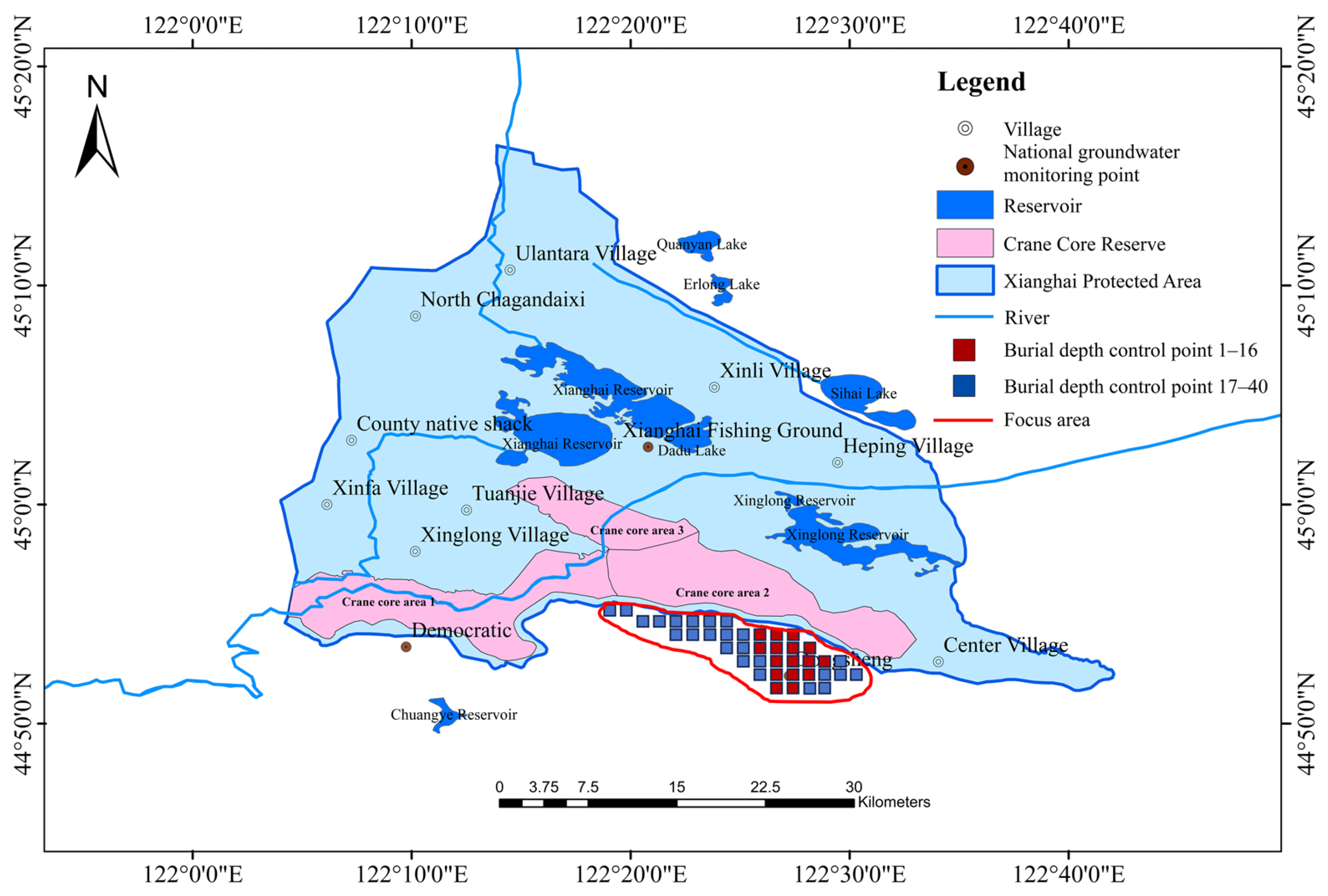
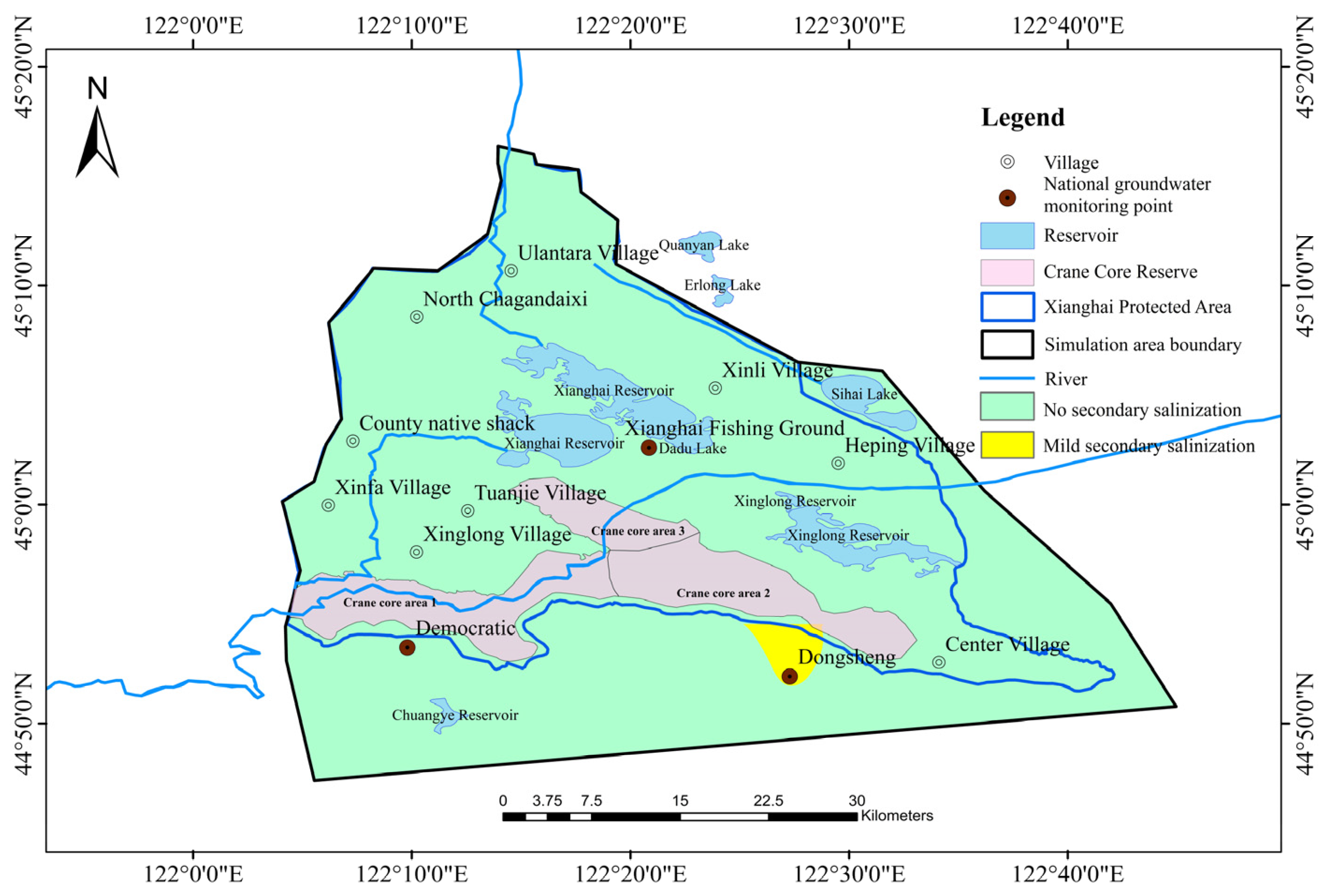
3.1. Study Area Overview

Located in Tongyu County, Baicheng City, in Northeast China, the Xianghai nature reserve is uniquely positioned in the heart of the vast Korqin Grassland. Its geographical coordinates range from 122°5′19″ to 122°31′38″ east longitude and 44°55′ to 45°09′ north latitude, covering an area of 1054 km2. The overview of the study area is depicted in Figure 3.
Xianghai nature reserve is an inland wetland and aquatic ecosystem type of nature reserve mainly aimed at protecting rare waterbirds like the red-crowned crane and valuable forest communities like the Mongolian elm. The primary responsibilities of the reserve include maintaining the wetlands and wetland ecosystems within the Korqin water system, Mutai River, Taoer River, and the Xianghai reservoir irrigation area, as well as the rich wildlife resources within the area. With the recent implementation of water supply projects, the reserve has established good engineering replenishment conditions. However, with the annual decrease in rainfall within the Taoer River basin in recent years, the deterioration of underlying surface conditions, and the lack of guaranteed upstream water supply, the water surface and swamp wetland area of the Xianghai reserve have gradually shrunk, with the wetland area having decreased by more than half. This poses a severe threat to the biodiversity of the reserve. Currently, the ecological water demand in the core area of the reserve exceeds the local water resources and the supply capacity of existing projects. To ensure sustainable development of the reserve, it is necessary to replenish water to the reserve. The monthly precipitation and evaporation in the study area are presented in Figure 4.
Replenishment can lead to an increase in the water table of the aquifer, reducing its burial depth, which, in turn, causes salinization. The formation and distribution of groundwater in the study area are governed by complex geological structures and natural factors. Prolonged sedimentation has produced thick sequences of clastic rocks and Quaternary unconsolidated deposits, facilitating groundwater storage. The main confined aquifers include the Upper Tertiary Da’an Formation (120–160 m depth), composed of gravelly mudstone and sandstone, and the Taikang Formation (45–90 m depth), characterized by highly permeable basal fine sandstone. Both formations are confined by interbedded mudstone aquitards. The Lower Pleistocene Baitushan Formation (24–80 m depth), dominated by gravel and sand layers, exhibits strong permeability and significant groundwater accumulation capacity. Unconfined groundwater within the Middle to Upper Pleistocene Quaternary deposits is extensively distributed, mainly stored in loess-like sandy silt and fine sand layers of the Upper Pleistocene Guxiangtun Formation. Despite its fine-grained texture, the formation remains loosely compacted, ensuring moderate permeability. This provides stable geological conditions for the formation and storage of unconfined groundwater, forming an aquifer with certain water supply potential. This study primarily focuses on the Quaternary pore aquifer, as the impact on the receiving area is predominantly observed in the unconfined aquifer, with minimal influence on the confined aquifer. The primary sources of groundwater recharge include precipitation infiltration, surface water infiltration, and lateral subsurface runoff, with the main discharge through evapotranspiration and lateral runoff. Overall, the groundwater exhibits a west-to-east flow trend, with a hydraulic gradient of approximately 1‰.
This article takes the Xianghai nature reserve as a case study area, proposing to replenish water in Crane Zones 2 and 3 from April to September each year over a period of 10 years. April-September was selected as the replenishment period because Xianghai serves as a reserve for cranes, and crane flocks only inhabit Xianghai from April to September. After September, the crane flocks begin to migrate southward, returning to Xianghai in April of the following year. Additionally, this period coincides with a period of high ecological activity, during which the ecosystem’s demand for water is relatively high. Replenishing water during this time can better meet the ecosystem’s needs, promoting ecosystem recovery and development.
As the replenishment progresses, the wetland area within the water-receiving zones will gradually expand. The soil in these wetlands will constantly maintain a certain layer of water. The movement of soil water and salt is predominantly downward. During the infiltration process, this water will leach the soil salts, diluting them and, thus reducing the soil salinity. The groundwater level around the water-receiving areas will rise. In the water-receiving areas (Crane Zones 2 and 3), the northern, western, and eastern sides predominantly consist of wetlands and reservoirs within the protected area, the surface will maintain a certain layer of water, and the groundwater movement will mainly be downward, making the leaching effect on soil salinity, not causing salinization. However, on the southern side of the water-receiving areas, in non-water areas, the elevated groundwater level under strong evaporation will increase the salt content in the soil surface, creating conditions for secondary salinization. Therefore, the focus is on the salinization issue on the southern side of the water-receiving areas. There are many factors contributing to soil salinization. For the receiving area, the main factor affecting changes before and after water replenishment is the burial depth of groundwater. Therefore, the primary consideration is the impact of groundwater depth on soil salinization.
To achieve the maximum total replenishment volume for the study area while maintaining a low degree of secondary salinization in the focus area after ten years of water replenishment, the replenishment is carried out up to the maximum available water capacity. First, the maximum available water supply is selected to predict the water supplementation for zones 2 and 3 of the crane habitat. To control the extent of salinization, the area of concern is defined as the region where the groundwater depth on the southern side of the water-receiving area is less than 2.5 m after 10 years of supplementation with the maximum available water supply. By setting depth control points in the focus area, where salinization is likely to occur, the groundwater depth after replenishment is controlled, thereby controlling the occurrence of salinization. The distribution of the focus area and depth control points is shown in Figure 5.

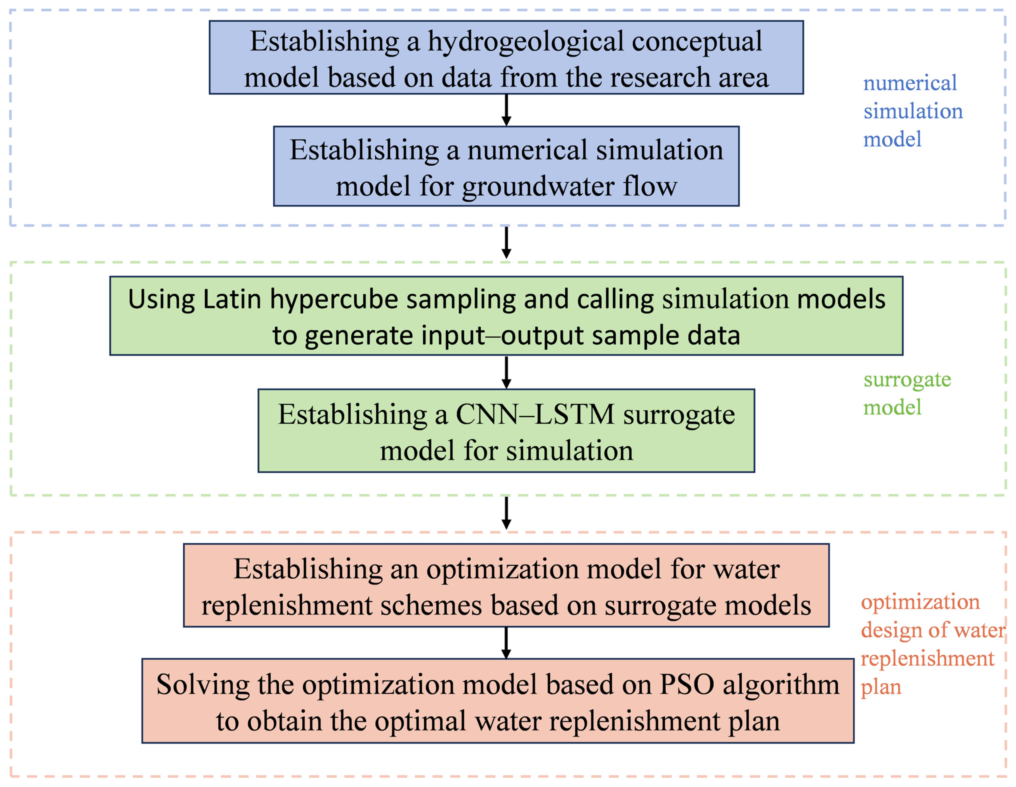
3.2. Construction of the Numerical Simulation Model

This study expanded the simulation area beyond the core of the protection zone, covering a region of approximately 1673.4 km2 (as shown in Figure 6). The target layer for this simulation calculation is the Quaternary unconsolidated rock porous phreatic aquifer. The water table in the research area is relatively flat, and the water flow is essentially horizontal, which allows for the vertical component of the seepage velocity to be ignored. Consequently, the flow is generalized as two-dimensional. The inputs and outputs of the groundwater system are influenced by precipitation infiltration, surface water infiltration, lateral subsurface runoff, evapotranspiration and extraction across different spatial and temporal scales. The groundwater level varies over time, and the groundwater flow is characterized by non-steady flow. The aquifer parameters do not vary significantly across space and are generalized as homogeneous. There is no significant directionality in the parameters, which can be generalized as isotropic. Summarizing the above, the groundwater flow system in the research area can be generalized as a homogeneous, isotropic, unsteady two-dimensional groundwater flow system. The calculation of source and sink terms is shown in Equations (13)–(17), where the precipitation infiltration recharge intensity and phreatic evaporation intensity are determined by the monthly precipitation and evaporation within the study area. These data are applied for a 10-year simulation period.
The calculation formula for precipitation infiltration recharge intensity is expressed as:
Q P R = α × P t
where Q P R represents the precipitation infiltration recharge intensity (m/d); α is the precipitation infiltration coefficient; P is the total precipitation within the study area (m); and t represents the calculation period in days (d).
The infiltration recharge intensity from rivers and lakes to groundwater can be expressed as:
Q L = K 1 h s h g d
where Q L is the infiltration recharge intensity from rivers and lakes (m/d); K 1 is the hydraulic conductivity of riverbed or lakebed sediments (m/d); h s is the water level of the river or lake (m); h g is the groundwater level (m); and d represents the thickness of riverbed or lakebed sediments (m).
The calculation formula for phreatic evaporation intensity is given as:
Q E R = Q E × C t
where Q E R represents the phreatic evaporation intensity (m/d); C is the phreatic evaporation coefficient; Q E is the total phreatic evaporation within the study area (m); and t is the calculation period in days (d).
The lateral recharge and discharge of groundwater along boundary zones can be estimated using Darcy’s Law, expressed as:
Q L R = K 2 × I × H × L × Δ t × sin θ
where Q L R represents the lateral groundwater recharge or discharge (m3); K 2 is the hydraulic conductivity of the aquifer (m/d); I is the hydraulic gradient of groundwater; H is the aquifer thickness (m); L is the width of the cross-sectional flow area (m); Δ t is the computation time step (d); and sin θ accounts for the angle between the groundwater flow direction and the cross-sectional boundary.
The groundwater extraction intensity is calculated as follows:
Q D = W A
where Q D represents the groundwater extraction intensity (m); W is the total groundwater extraction volume (m3); and A is the area of the extraction region (m2).
The upper boundary of the simulation area is the groundwater surface, a continually changing boundary for water exchange, including precipitation infiltration and evapotranspiration across. The bottom boundary of the simulation area is the impermeable mudstone layer, generalized as a no-flow boundary. The western part of the simulation area is the lateral inflow boundary, and the northeastern side is the lateral outflow boundary, both generalized as known flow boundaries. The southern boundary is parallel to the flow lines and generalized as a no-flow boundary.
According to the available hydrogeological data, the initial values of hydrogeological parameters are determined as shown in Table 1.
Based on the hydrogeological conceptual model, the homogeneous, isotropic, and unsteady two-dimensional groundwater flow system can be described by the following partial differential equation and its boundary conditions:
x ( H Z ) H x + y ( H Z ) H y + W K = μ K H t , ( x , y ) Ω , t 0 H x , y , t t = 0 = H 0 x , y , x , y Ω , t = 0 K H Z H n Γ 2 = q x , y , t , x , y Γ 2 , t > 0 K H n Γ 3 = 0 , x , y Γ 3 , t > 0
where H is the groundwater level; H 0 ( x , y ) is the initial water level; Z is the elevation of the target aquifer floor; K is the permeability coefficient; μ is the specific yield; W is the vertical recharge and discharge intensity of the phreatic aquifer; Γ 2 is the known flow boundary; q ( x , y , t ) is the lateral single width displacement of the aquifer; Γ 3 is the impermeable boundary; n is the direction of the outer normal on the boundary; and Ω is the simulation calculation area.
Utilizing the MODFLOW module within GMS software, the aforementioned mathematical model is solved. In the simulation computation area, a rectangular partition is employed, dividing the area into 1784 finite difference grids, with each cell measuring 1000 m × 1000 m. The simulation spans 10 years and is discretized into 200-time steps.
In this study, a local sensitivity analysis method was employed to identify the parameters that have a significant impact on the model outputs. Local sensitivity analysis is used to investigate the influence of variations in individual parameters on the results of numerical simulations. During the analysis, only the parameter under investigation is varied, while all other parameters are kept constant. The main advantages of this approach are its simplicity and ease of implementation, as well as the preservation of computational accuracy. The corresponding formula is as follows:
X k = y / a k
where X k denotes the sensitivity coefficient, which quantifies the influence of changes in parameter a k on the model output y .
When calculating the sensitivity coefficient for parameter k , all other parameters are kept constant. The value of parameter k is changed from a k to α k + Δ a k , resulting in a change in the dependent variable from y i α k to y i α k + Δ a k . The sensitivity coefficient is then computed using the following equation:
X i , k = y i a k y i α k + Δ a k y i α k / Δ a k
X k = y a k   y α k + Δ a k y α k / y α k / Δ a k / α k
Equation (21) is the calculation formula without considering units.
The parameters involved in this sensitivity analysis are the hydraulic conductivity K , specific yield μ , and atmospheric precipitation infiltration coefficient α . The values of these three parameters are listed in 
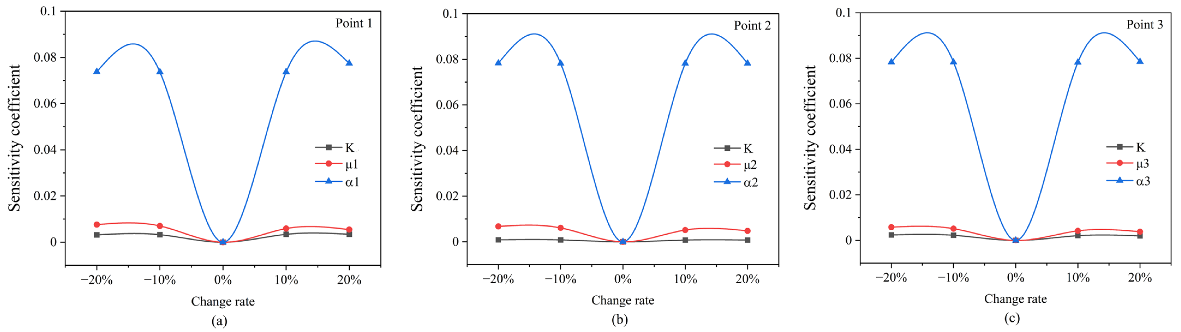
Table 1. Each parameter was individually increased and decreased by 10% and 20%. Three representative groundwater burial depth control points (Figure 7) were selected from the focus area, corresponding to the westernmost (Point 1), easternmost (Point 2), and southernmost (Point 3) locations. Using Equation (21), the sensitivity analysis was conducted with the groundwater table at three control points after 10 years of recharge as the output variable. The results of the sensitivity analysis are presented in Table 2 and Figure 8.
As shown in Figure 8, the results of the local sensitivity analysis indicate that for all three control points, the atmospheric precipitation infiltration coefficient α is the most influential parameter.
To ensure mesh independence and the reliability of the model results, sensitivity analyses on different mesh sizes were conducted. Specifically, grid resolutions of 500 m × 500 m, 1000 m × 1000 m, and 1500 m × 1500 m were tested under identical boundary and initial conditions. The groundwater levels at key monitoring points after ten years of simulation were compared for these mesh configurations. Using the 500 m × 500 m grid as the reference, the relative differences in groundwater levels for the other mesh sizes are presented in Table 3.
The results show that the relative differences between the 500 m × 500 m and 1000 m × 1000 m grids were less than 0.5%, indicating negligible sensitivity to grid resolution refinement. However, increasing the mesh size to 1500 m × 1500 m introduced deviations exceeding 0.5%, suggesting insufficient accuracy at this scale. Therefore, a grid resolution of 1000 m × 1000 m was selected as mesh independent and used consistently throughout this study.
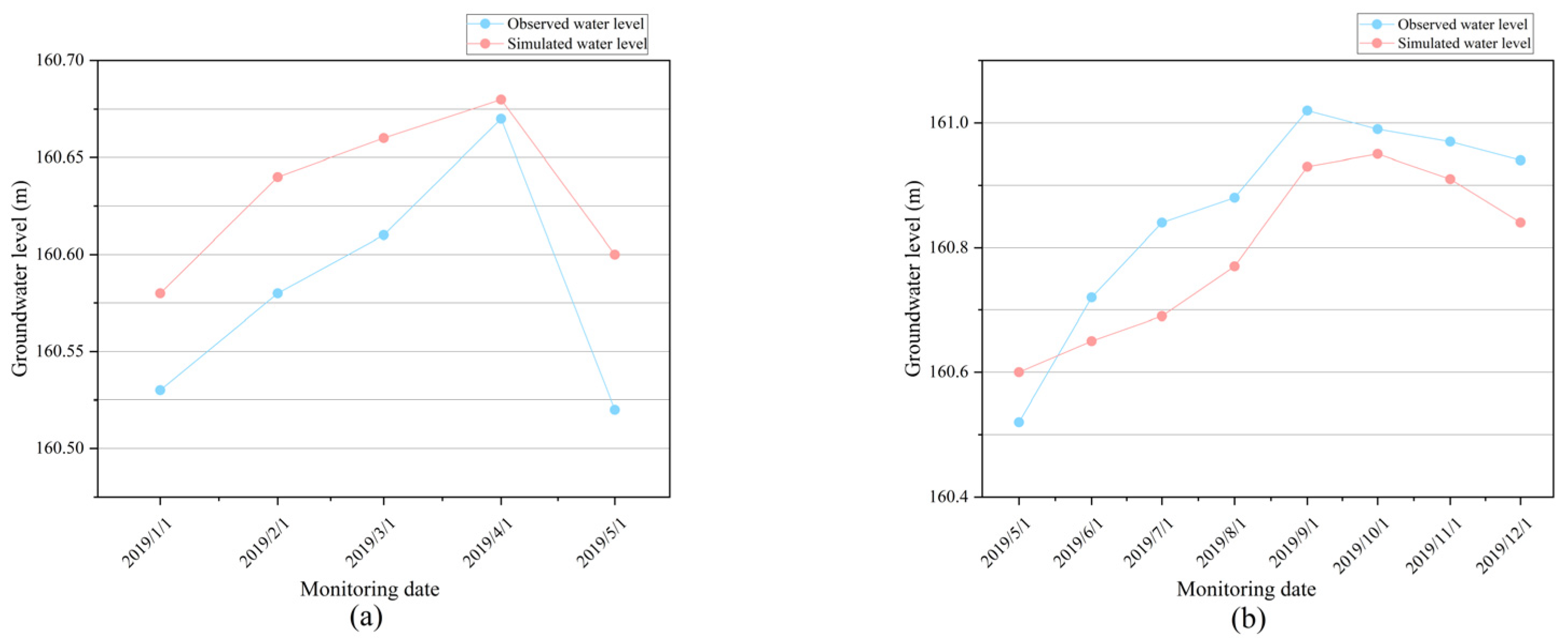
Based on the results of the local sensitivity analysis, this study utilizes the existing water level monitoring data to identify model parameters and verify model reliability. The identification period is from 1 January 2019 to 1 May 2019, and the validation period is from 1 May 2019 to 1 December 2019. The water level fitting results of the monitoring wells during the identification and verification periods are shown in Figure 9, Figure 10 and Figure 11 below. The hydrogeological parameters identified and validated are as shown in Table 4.
From the water level fittings in Figure 9, Figure 10 and Figure 11, it can be observed that the overall fit between the modeled water level results during the identification and verification periods and the actual measured results is quite high. Additionally, the dynamic fitting of the monitoring points illustrates that the deviation between the measured and simulated water levels at the monitoring points is less than 0.2 m, and their dynamic trends are generally consistent. In summary, the established simulation model reliably simulates hydrogeological conditions and groundwater flow fields.

3.3. Construction of the Surrogate Model

The Latin hypercube sampling method was used to sample 12 input variables (monthly water replenishment volumes for crane species zones 2 and 3 from April to September), extracting 100 uniformly distributed samples as input values. These 100 groups of sample input values were then entered into the developed groundwater numerical model for computation, obtaining 100 groups of water table depth data after 10 years at 40 buried depth control points as the sample output values. These 100 groups of samples were used as the training set. Similarly, using the random sampling method, 50 sets of samples were drawn for the 12 input variables as input values, and the corresponding output values were obtained using GMS software, forming the validation set.
A CNN-LSTM neural network was utilized to establish a surrogate model for the simulation model, using the input–output sample set to train the deep learning neural network.

3.4. Construction of the Optimization Model

The optimization model consists of three components: decision variables, objective function, and constraints. The monthly water replenishment volumes for Crane Zones 2 and 3 from April to September were used as decision variables.

3.4.1. Objective Function

The maximization of the total water replenishment volume from April to September for Crane Zones 2 and 3 as the objective function is as follows:
m a x Z = j = 2 3 t = 4,5 , 6,7 , 8,9 Q j , t
where Z is the total replenishment volume, and Q j , t is the water replenishment amount of j-th crane area in t-th month.

3.4.2. Constraint Conditions

The ecological water demand for Crane Zone 2 and Crane Zone 3, available water supply, post-replenishment observation point water table depth, and the established CNN-LSTM surrogate model serve as constraint conditions.
(1)
Ecological water demand constraints
Q j , t Q j , t m i n , j = 2,3 ; t = 4,5 9
Here, Q j , t m i n is the ecological water demand. The ecological water demand requirements are shown in Table 5.
(2)
Water supply constraints
j = 2 3 Q j , t Q j , t m a x , j = 2,3 ; t = 4,5 9
Here, Q j t m a x is the available water supply. The available water volume requirements are shown in Table 6.
(3)
Water level depth constraint considering the problem of secondary soil salinization
The existing literature indicates [41] that in the western region of Jilin Province, when the burial depth exceeds 2.5 m, salinization does not occur. However, when the burial depth ranges from 2 to 2.5 m, mild salinization and alkalinization can occur. Therefore, to ensure the prevention of salinization, it is required that all monitoring points in the focus area have a burial depth greater than 2.5 m. From the initial burial depth map dated 1 December 2020 (Figure 12), it can be observed that the burial depth near Dongsheng is smaller than in other areas, so the requirements for burial depth in this area can be relaxed. The specific constraints on burial depth are as follows:
d i , 10 d i , m i n = 2.5 , i = 17,18 40 d i , 10 d i , m i n = 2 , i = 1,2 16
where d i , 10 is the water level burial depth of observation point i after 10 years, and d i , m i n is the minimum water level burial depth of observation point i .
(4)
Equality constraints constituted by the surrogate model
d i , 10 = M ( Q j , t )
Here, d i , 10 is a function of the replenishment volume, representing the simulated water table depth at observation point i after 10 years, which is predicted by the established surrogate model M derived from numerical simulation model.

4. Results and Discussion

4.1. Analysis of Surrogate Model Results

To construct the surrogate models, the main hyper-parameters of the CNN-LSTM neural network and Kriging method were carefully selected, as summarized in Table 7 and Table 8, respectively. For the CNN-LSTM neural network (Table 7), the number of CNN layers (2) controls the complexity and depth of feature extraction from input data, while the kernel size (3) determines the local scope of data processed by convolution operations. The number of channels (24) defines the number of output feature maps, influencing the richness and dimensionality of the extracted features. The LSTM units (48) indicate the number of neurons in the LSTM layer, enhancing the model’s capacity to capture temporal dependencies in sequential data. A dropout rate of 0.3 was used to reduce overfitting by randomly deactivating a fraction of neurons during training. Additionally, the model was trained for 1000 epochs to achieve convergence, with a learning rate of 0.001 to control the parameter update speed during optimization. For the Kriging surrogate model (Table 8), the regression function selected was constant, assuming a uniform baseline trend across the input space. The ARD Squared Exponential correlation function was applied to effectively capture the nonlinear spatial relationships between input points, with correlation function parameters automatically optimized during model training. Based on these configurations, the CNN-LSTM surrogate model was trained, and the fitting results for the training and test sets are shown in Figure 13. For comparison, the performance of the trained Kriging surrogate model is presented in Figure 14.
From the fitting results shown in Figure 13 and Figure 14, it can be observed that the CNN-LSTM neural network surrogate model achieves excellent fitting accuracy, with an R-squared (R2) value of 0.9996 and a mean relative error (MRE) of 0.0023 for the training set and an R2 of 0.9962 and MRE of 0.0089 for the test set. Most of the fitted data points are closely concentrated along the 1:1 line, indicating a high level of agreement between the CNN-LSTM surrogate model and the numerical simulation model. In contrast, the Kriging model yields R2 values of 0.9885 (training set) and 0.8023 (test set), with corresponding MREs of 0.0174 and 0.4073, showing that while Kriging performs reasonably for the training set, its accuracy drops markedly for the test set as data points deviate further from the 1:1 line. This comparison demonstrates that the CNN-LSTM model provides superior generalization ability and predictive performance compared to the traditional Kriging surrogate model, making it more suitable to replace the numerical groundwater simulation model for computational purposes in this study. The relative error is calculated by taking the difference between the simulated model results vs. the predicted results from the CNN-LSTM surrogate model. The distribution of relative errors is shown in Figure 15.
Figure 15 shows that the relative error follows a normal distribution, with a mean close to 0 and a small variance. The relative error is tightly distributed between −2% and 2%, with most of the errors concentrated around 0, indicating low dispersion. The high concentration and low variance of the data suggest that the surrogate model established by the CNN-LSTM neural network has a high prediction accuracy.

4.2. Analysis of the Optimization Results for the Water Replenishment Scheme

The replenishment plan was obtained by solving the optimization model 20 times using the Particle Swarm Optimization algorithm and averaging the results. The primary hyper-parameters of the PSO algorithm are summarized in Table 9. For the PSO algorithm (Table 9), the swarm size (50) defines the number of particles searching for optimal solutions simultaneously, while the dimension (12) corresponds to the number of decision variables (monthly replenishment volumes). The algorithm was set to perform a maximum of 100 iterations to balance solution quality with computational cost. The inertia weight dynamically adjusted from 0.9 to 0.2 encourages initial global exploration and subsequent local exploitation. The cognitive and social coefficients were both set to 1.5, balancing individual particle experience with group knowledge to guide the optimization process effectively. A histogram of the replenishment plan results for each iteration, along with the average result, was plotted, and the standard deviation was calculated, as shown in Figure 16.
From Figure 16, it can be observed that the water replenishment volumes for Crane Zone 2 in April, June, and September, as well as for Crane Zone 3 in August and September, remain constant across each calculation iteration, with a standard deviation of 0. Therefore, using the average values can effectively represent the water replenishment volumes for these months. For Crane Zone 2 in May, July, and August, as well as for Crane Zone 3 in April, May, June, and July, the water replenishment volumes exhibit minor variations across each calculation iteration, with deviations from the average values being minimal and a small standard deviation, indicating relatively concentrated results. This implies that the average values can adequately represent the overall level of these computed results while also demonstrating the stability of the algorithm. The average value of the replenishment scheme can be considered the optimal replenishment scheme to supply water to crane species zones 2 and 3 in the Xianghai nature reserve.
The total replenishment volume of the optimal replenishment plan is 7446.78 × 104 m3. The results of the replenishment plan are shown in Table 10.

4.3. Verification of Water Replenishment Plan Optimization Results

To verify the impact of the optimal water replenishment plan on the secondary salinization in the study area, the optimal plan (as detailed in Table 10) was input into the numerical model. This model was then run to determine the extent of secondary salinization after 10 years of water replenishment under this plan (as shown in Figure 17).
According to Figure 17, after ten years of water replenishment using the optimal plan, only the area around Dongsheng and its northern part within a 2.5 km radius experiences mild secondary salinization. Other areas do not undergo secondary salinization, adhering to the depth constraint. This ensures that the degree of secondary salinization in the study area remains as low as possible after ten years of replenishment.
To demonstrate the superiority of the optimal water replenishment scheme, we distribute the same total amount of water (7446.78 × 104 m3) as in the optimized scheme evenly across all regions and time periods. The secondary salinization condition after ten years of replenishment under this evenly distributed plan (as shown in Figure 18) is compared with that of the optimal water replenishment plan.
According to Figure 18, after ten years of water replenishment using the evenly distributed water supply plan, not only does the area near Dongsheng in the southern part of the water-receiving area experience mild secondary salinization, but also a zone approximately 1.5 km north of Dongsheng undergoes about 1 km2 of moderate secondary salinization. This scenario does not meet the depth constraint condition. Compared to the optimal water replenishment plan, the evenly distributed water supply plan results in a higher degree of secondary salinization in the focus area, leading not only to mild but also to moderate salinization, and it does not minimize the extent of secondary salinization in the region nor satisfy the depth constraint condition.
Therefore, using the optimal water replenishment plan can maximize the total volume of water replenished while keeping the degree of secondary salinization in the study area as low as possible after ten years of replenishment. This plan provides a scientific basis for ecological water replenishment in the Xianghai nature reserve.

4.4. Discussion

To further elucidate the contributions and prospects of this study, the main methodological strengths and directions for future research are outlined below.

4.4.1. Benefit and Advantages of the Adopted Methods

The simulation–optimization framework developed in this study exhibits several notable advantages for ecological water replenishment management in salinity-prone wetland environments:
(1)
Direct incorporation of salinization constraints: The framework explicitly incorporates secondary soil salinization as a constraint in the optimization process. By doing so, it addresses a critical but often overlooked challenge in wetland water management, ensuring that ecological restoration efforts do not inadvertently exacerbate soil degradation.
(2)
Facilitation of science-based management: The approach provides stakeholders and practitioners with a robust, quantitative tool for balancing ecological water needs with environmental constraints. This is especially relevant for regions where wetland sustainability is threatened by both water scarcity and soil salinization.

4.4.2. Implications for Future Research

This simulation–optimization framework provides a scientific basis for wetland management in salinity-prone environments and can be adapted to other regions with similar hydrogeological and ecological settings. Future studies may improve the framework in the following ways:
(1)
In future work, we will incorporate longer-term groundwater level monitoring data to continuously validate and update the model, thereby enhancing its reliability.
(2)
We will conduct a more refined analysis of aquifer heterogeneity, investigating how the characterization of spatial variability in hydrogeological parameters influences the simulation and optimization results. Incorporating detailed descriptions of aquifer heterogeneity will help enhance the physical realism and applicability of the model under more complex site conditions.
(3)
Although the current study focuses primarily on ecological criteria, future research should consider integrating the water needs and preferences of local stakeholders, including farmers, residents, and industries. Modeling and multi-objective optimization can help balance ecological, social, and economic outcomes.

5. Conclusions

This paper focuses on the Xianghai nature reserve, employing simulation-optimization, CNN-LSTM neural networks, and PSO optimization algorithms to obtain a water management strategy that maximizes the total replenishment volume over ten years while minimizing the degree of secondary soil salinization in the study area. The proposed optimization framework not only effectively controls soil salinity and supports wetland health but can also be adapted to meet local water use demands. The main conclusions are as follows:
(1)
The surrogate model established using the CNN-LSTM neural network can well approximate the input–output relationship of the simulation model, with an R2 of 0.99 and a significantly faster operation speed than the numerical simulation model, proving that it can replace the numerical simulation model embedded in the optimization model for designing water replenishment schemes.
(2)
The use of the Particle Swarm Optimization (PSO) algorithm to repeatedly solve for monthly replenishment volumes shows minimal variation in results, and the deviations from the mean are close to zero and have low standard deviations, indicating that the results are relatively concentrated. This demonstrates the strong stability of this optimization algorithm.
(3)
Compared to a randomized approach, the proposed management scheme significantly improves soil salinity control. After a ten-year period, only mild salinity was detected within 2.5 km north of Dongsheng, while the random scheme resulted in both mild and moderate salinity issues, affecting approximately 1 km2 located 1.5 km farther north. This demonstrates the clear advantage of the proposed optimization approach and provides a strong reference for future ecological water management efforts.

Author Contributions

Z.S.: Conceptualization, Methodology, Software, Formal analysis, Writing—original draft, Writing—review and editing, and Visualization. J.L.: Methodology, Software, Formal analysis, Data curation, Writing—original draft, Writing—review and editing, and Funding acquisition. X.M.: Data curation and Writing—review and editing. All authors have read and agreed to the published version of the manuscript.

Funding

This study is supported by the National Natural Science Foundation of China (No. 42472317).

Data Availability Statement

Data will be made available on request.

Conflicts of Interest

The authors declare no conflicts of interest.

Code Availability Section

Name of the code/library: WaterReplenishmentScheme. Contact: 1070662769@qq.com; +8613308675957. Hardware requirements: Intel CPU and NVIDIA GPU. Program language: Matlab. Software required: Matlab R2021b. Program size: 11 KB. The source codes are available for downloading at the link: https://github.com/songzhuo24/WaterReplenishmentScheme (accessed on 17 June 2025).

References

  1. Busch, D.E.; Loftus, W.F.; Bass, O.L. Long-term hydrologic effects on marsh plant community structure in the southern Everglades. Wetlands 1998, 18, 230–241. [Google Scholar] [CrossRef]
  2. Mao, D.; Wang, Z.; Wu, J.; Wu, B.; Zeng, Y.; Song, K.; Yi, K.; Luo, L. China’s wetlands loss to urban expansion. Land Degrad. Dev. 2018, 29, 2644–2657. [Google Scholar] [CrossRef]
  3. Li, D.; Zhu, S.; Gao, J.; Jiang, H.; Deng, G.; Sheng, L.; Cao, Y.; Li, L.; Lin, B. The influence of ecological engineering on waterbird diversity in different habitats within the Xianghai Nature reserve. Diversity 2022, 14, 1016. [Google Scholar] [CrossRef]
  4. Sheng, L.; He, C.; Zhao, J.; Song, Y.; Zou, L. Analysis of effect of wetland ecological environment change in Xianghai nature reserve on number and distribution of Red-crowned Crane. J. Northeast Norm. Univ. (Nat. Sci. Ed.) 2001, 33, 91–93. [Google Scholar] [CrossRef]
  5. Wang, G.P.; Liu, J.S.; Tang, J. The long-term nutrient accumulation with respect to anthropogenic impacts in the sediments from two freshwater marshes (Xianghai Wetlands, Northeast China). Water Res. 2004, 38, 4462–4474. [Google Scholar] [CrossRef]
  6. Wang, G.; Zhang, Y. Impacts of reservoir project on hydrologial and ecologial environment of Xianghai wetlands. Resour. Sci. 2002, 24, 26–30. [Google Scholar] [CrossRef]
  7. Zhang, H.; Long, E.; Cheng, W. Research on dynamic change and effect factors of Xianghai Wetland. J. Nat. Resour. 2005, 20, 613–620. [Google Scholar] [CrossRef]
  8. Guo, Y.; Huang, S.; Huang, Q.; Wang, H.; Fang, W.; Yang, Y.; Wang, L. Assessing socioeconomic drought based on an improved Multivariate Standardized Reliability and Resilience Index. J. Hydrol. 2019, 568, 904–918. [Google Scholar] [CrossRef]
  9. Metternicht, G.; Zinck, A. Remote Sensing of Soil Salinization: Impact on Land Management; CRC Press: Boca Raton, FL, USA, 2008. [Google Scholar]
  10. Metternicht, G.; Zinck, J.A. Spatial discrimination of salt- and sodium-affected soil surfaces. Int. J. Remote Sens. 1997, 18, 2571–2586. [Google Scholar] [CrossRef]
  11. Morshed, J.; Kaluarachchi, J.J. Enhancements to genetic algorithm for optimal ground-water management. J. Hydrol. Eng. 2000, 5, 67–73. [Google Scholar] [CrossRef]
  12. Yakowitz, S. Dynamic programming applications in water resources. Water Resour. Res. 1982, 18, 673–696. [Google Scholar] [CrossRef]
  13. Duan, H.; Xu, M.; Cai, Y.; Wang, X.; Zhou, J.; Zhang, Q. A holistic wetland ecological water replenishment scheme with consideration of seasonal effect. Sustainability 2019, 11, 930. [Google Scholar] [CrossRef]
  14. Wang, W.; Hu, P.; Yang, Z.; Wang, J.; Zhao, J.; Zeng, Q.; Liu, H.; Yang, Q. Prediction of NDVI dynamics under different ecological water supplementation scenarios based on a long short-term memory network in the Zhalong Wetland, China. J. Hydrol. 2022, 608, 127626. [Google Scholar] [CrossRef]
  15. Loftis, B. Optimal Operation of a System of Lakes for Quality and Quantity. Ph.D. Thesis, Colorado State University, Fort Collins, CO, USA, 1985. [Google Scholar]
  16. Xu, Y.; Wang, Y.; Li, S.; Huang, G.; Dai, C. Stochastic optimization model for water allocation on a watershed scale considering wetland’s ecological water requirement. Ecol. Indic. 2018, 92, 330–341. [Google Scholar] [CrossRef]
  17. Yang, H.; He, W.; Li, Y. Optimization of ecological water replenishment scheme based on the interval fuzzy two-stage stochastic programming method: Boluo lake national nature reserve, Jilin Province, China. Int. J. Environ. Res. Public Health 2022, 19, 5218. [Google Scholar] [CrossRef]
  18. Dadaser-Celik, F.; Coggins, J.S.; Brezonik, P.L.; Stefan, H.G. The projected costs and benefits of water diversion from and to the Sultan Marshes (Turkey). Ecol. Econ. 2009, 68, 1496–1506. [Google Scholar] [CrossRef]
  19. Karamouz, M.; Mojahedi, S.A.; Ahmadi, A. Interbasin water transfer: Economic water quality-based model. J. Irrig. Drain. Eng. 2010, 136, 90–98. [Google Scholar] [CrossRef]
  20. Qiu, Y.; Liu, Y.; Liu, Y.; Chen, Y.; Li, Y. An interval two-stage stochastic programming model for flood resources allocation under ecological benefits as a constraint combined with ecological compensation concept. Int. J. Environ. Res. Public Health 2019, 16, 1033. [Google Scholar] [CrossRef]
  21. Alafifi, A.H.; Rosenberg, D.E. Systems modeling to improve river, riparian, and wetland habitat quality and area. Environ. Modell. Softw. 2020, 126, 104643. [Google Scholar] [CrossRef]
  22. Huang, J.; Zhao, L.; Sun, S. Optimization model of the ecological water replenishment scheme for boluo lake national nature reserve based on interval two-stage stochastic programming. Water 2021, 13, 1007. [Google Scholar] [CrossRef]
  23. Jiang, H.; He, C.; Luo, W.; Yang, H.; Sheng, L.; Bian, H.; Zou, C. Hydrological restoration and water resource management of Siberian Crane (Grus leucogeranus) Stopover Wetlands. Water 2018, 10, 1714. [Google Scholar] [CrossRef]
  24. Cai, B.; Meng, C.; Wang, X.E.; Li, Y. Application of a fuzzy two-stage chance constrained stochastic programming model for optimization of the ecological services value of the interconnected river system network project in the Western Jilin Province, China. Water 2019, 11, 68. [Google Scholar] [CrossRef]
  25. Yinglan, A.; Wang, J.; Zeng, Q.; Wu, S.; Yan, L.; Liu, H.; Yang, Z.; Yang, Q.; Wang, L.; Hu, P. Optimization of wetland water replenishment process based on the response of waterbirds in a semi-arid and cold region. Ecol. Indic. 2023, 156, 111142. [Google Scholar] [CrossRef]
  26. Asher, M.J.; Croke, B.F.W.; Jakeman, A.J.; Peeters, L.J.M. A review of surrogate models and their application to groundwater modeling. Water Resour. Res. 2015, 51, 5957–5973. [Google Scholar] [CrossRef]
  27. Luo, J.; Lu, W.; Yang, Q.; Ji, Y.; Xin, X. An adaptive dynamic surrogate model using a constrained trust region algorithm: Application to DNAPL-contaminated-groundwater-remediation design. Hydrogeol. J. 2020, 28, 1285–1298. [Google Scholar] [CrossRef]
  28. Luo, J.; Lu, W. Comparison of surrogate models with different methods in groundwater remediation process. J. Earth Syst. Sci. 2014, 123, 1579–1589. [Google Scholar] [CrossRef]
  29. Queipo, N.V.; Haftka, R.T.; Shyy, W.; Goel, T.; Vaidyanathan, R.; Kevin Tucker, P. Surrogate-based analysis and optimization. Prog. Aerosp. Sci. 2005, 41, 1–28. [Google Scholar] [CrossRef]
  30. Razavi, S.; Tolson, B.A.; Burn, D.H. Review of surrogate modeling in water resources. Water Resour. Res. 2012, 48. [Google Scholar] [CrossRef]
  31. Xiong, Y.; Luo, J.; Liu, X.; Liu, Y.; Xin, X.; Wang, S. Machine learning-based optimal design of groundwater pollution monitoring network. Environ. Res. 2022, 211, 113022. [Google Scholar] [CrossRef]
  32. McKay, M.D.; Beckman, R.J.; Conover, W.J. A comparison of three methods for selecting values of input variables in the analysis of output from a computer code. Technometrics 1979, 21, 239–245. [Google Scholar] [CrossRef]
  33. Liu, Y.; Luo, J.; Xiong, Y.; Ji, Y.; Xin, X. Inversion of hydrogeological parameters based on an adaptive dynamic surrogate model. Hydrogeol. J. 2022, 30, 1513–1527. [Google Scholar] [CrossRef]
  34. He, W.; Wang, X.; Zhang, Y.; Zhu, B.; Wu, H. Adsorption behavior of aged polystyrene microplastics (PSMPs) for manganese in water: Critical role of hydrated functional zone surrounding the microplastic surface. J. Environ. Chem. Eng. 2022, 10, 109040. [Google Scholar] [CrossRef]
  35. Nguyen, H.V.; Pham, T.X.; Le, C.N. Real-time long short-term glance-based fire detection using a CNN-LSTM neural network. Int. J. Intell. Inf. Database Syst. 2021, 14, 349–364. [Google Scholar] [CrossRef]
  36. Jahandideh-Tehrani, M.; Jenkins, G.; Helfer, F. A comparison of particle swarm optimization and genetic algorithm for daily rainfall-runoff modelling: A case study for Southeast Queensland, Australia. Optim. Eng. 2021, 22, 29–50. [Google Scholar] [CrossRef]
  37. Chen, H.-T.; Wang, W.-C.; Chen, X.-N.; Qiu, L. Multi-objective reservoir operation using particle swarm optimization with adaptive random inertia weights. Water Sci. Eng. 2020, 13, 136–144. [Google Scholar] [CrossRef]
  38. Jahandideh-Tehrani, M.; Bozorg-Haddad, O.; Loáiciga, H.A. Application of particle swarm optimization to water management: An introduction and overview. Environ. Monit. Assess. 2020, 192, 281. [Google Scholar] [CrossRef]
  39. Zhang, G.-H.; Liu, X.-D.; Wu, S.; Hua, Z.-L.; Zhao, L.; Xue, H.-Q.; Wang, P. Identification of pollution sources in river based on particle swarm optimization. J. Hydrodyn. 2021, 33, 1303–1315. [Google Scholar] [CrossRef]
  40. Wu, Z.; Yin, L.; Xiong, R.; Wang, S.; Xiao, W.; Liu, Y.; Jia, J.; Liu, Y. A novel state of health estimation of lithium-ion battery energy storage system based on linear decreasing weight-particle swarm optimization algorithm and incremental capacity-differential voltage method. Int. J. Electrochem. Sci. 2022, 17, 220754. [Google Scholar] [CrossRef]
  41. Cui, X. Study on the Groundwater and Environment Influenced by Water Diversion Irrigation in Week Eco-Environmental Area of Zhenlai County. Master’s Thesis, Jilin University of Technology, Changchun, China, 2008. [Google Scholar]
Figure 1. Design framework for the water replenishment scheme.
Water 17 01886 g001
Figure 3. Overview of the study area.
Water 17 01886 g003
Figure 4. Monthly precipitation and evaporation charts of the study area. (a) Monthly precipitation in the study area and (b) monthly evaporation in the study area.
Water 17 01886 g004
Figure 5. Layout diagram of buried depth control points.
Water 17 01886 g005
Figure 6. Boundary conditions diagram.
Water 17 01886 g006
Figure 7. Schematic diagram of control point locations.
Water 17 01886 g007
Figure 8. Local sensitivity analysis results for the three control points: (a) Point 1, (b) Point 2, and (c) Point 3.
Water 17 01886 g008
Figure 9. Fitting results of the groundwater level at the end of the identification period.
Water 17 01886 g009
Figure 10. Fitting results of the groundwater level at the end of the validation period.
Water 17 01886 g010
Figure 11. Dynamic fitting results of groundwater level in monitoring wells: (a) identification period and (b) verification period.
Water 17 01886 g011
Figure 12. Initial distribution of groundwater burial depth.
Water 17 01886 g012
Figure 13. Fitting results of the CNN-LSTM neural network: (a) training set and (b) test set.
Water 17 01886 g013
Figure 14. Fitting results of the Kriging model: (a) training set and (b) test set.
Water 17 01886 g014
Figure 15. The relative error distribution diagram of the CNN-LSTM surrogate model.
Water 17 01886 g015
Figure 16. Histogram of water replenishment scheme: (a) histogram of water replenishment (volume for Crane Zone 2) and (b) histogram of water replenishment (volume for Crane Zone 3).
Water 17 01886 g016
Figure 17. Secondary salinization condition after 10 years of water replenishment under the optimal plan.
Water 17 01886 g017
Figure 18. Secondary salinization condition after 10 years of water replenishment using the evenly distributed water supply plan.
Water 17 01886 g018
Table 1. The initial values of hydrogeological parameters table.
ParameterNumerical Value
Hydraulic conductivity10 m/d
Specific yield0.065
Atmospheric precipitation infiltration coefficient0.15
Table 2. Sensitivity analysis results of different parameters at each point.
Parameter Change Rate
−20%−10%010%20%
K 0.003160.0032700.003420.00346
μ 1 0.007620.0070200.005920.00548
α 1 0.07380.073700.07370.0774
K 0.000860.0008300.000780.00077
μ 2 0.006740.0061000.005150.00478
α 2 0.07830.078200.07820.0782
K 0.002380.0022600.002070.00198
μ 3 0.005810.0051600.004190.00382
α 0.07830.078300.07820.0785
Table 3. The relative errors of different grid sizes.
Grid SizeRelative Error Point 1 (%)Relative Error Point 2 (%)Relative Error Point 3 (%)
500 m × 500 m---
1000 m × 1000 m0.0862%0.2452%0.4051%
1500 m ×1500 m0.2377%0.5152%0.8385%
Table 4. Results of identification and validation of hydrogeological parameters.
ParameterNumerical Value
Hydraulic conductivity12 m/d
Specific yield0.05
Atmospheric precipitation infiltration coefficient0.15
Table 5. Ecological water demand (×104 m3).
AreaEcological Water Demand
AprilMayJuneJulyAugustSeptember
Crane Zone 2722872705488670686
Crane Zone 3289348280192267274
Table 6. Available water supply (×104 m3).
Available Water Supply
AprilMayJuneJulyAugustSeptember
150015001500150015001500
Table 7. The main hyper-parameters of the CNN-LSTM surrogate model.
Hyper-ParameterNumber of CNN LayersKernel SizeNumber of ChannelsLSTM UnitsDropout RateEpochsLearning Rate
Value2324480.310000.001
Table 8. The main hyper-parameters of the Kriging surrogate model.
Hyper-ParameterRegression
Function
Correlation
Function
Correlation Function Parameters
ValueConstantARD Squared Exponential σ (Sigma) = 0.001, θ 1 ,   θ 2 ,…, θ 12 (optimized automatically)
Table 9. The main hyper-parameters of the PSO algorithm.
Hyper-ParameterSwarm SizeDimensionMax IterationsCognitive CoefficientSocial CoefficientInertia Weight
Value50121001.51.50.9–0.2 (linear)
Table 10. Optimal water replenishment scheme (×104 m3).
AreaWater Replenishment Volume
AprilMayJuneJulyAugustSeptember
Crane Zone 2722936.33705703.5744.12686
Crane Zone 3498.72422.92499.43498.76500500
Disclaimer/Publisher’s Note: The statements, opinions and data contained in all publications are solely those of the individual author(s) and contributor(s) and not of MDPI and/or the editor(s). MDPI and/or the editor(s) disclaim responsibility for any injury to people or property resulting from any ideas, methods, instructions or products referred to in the content.

