Prediction of Sluice Seepage Based on Impact Factor Screening and the IKOA-BiGRU Model

Abstract

Sluices play a critical role in flood control, power generation, water supply, etc. With decades of service, sluice safety assurance becomes a structural engineering imperative. Previous investigations have revealed that failures of sluices are often associated with seepage damage. To gain further insight into sluice seepage and ensure the safety of sluice structures, proposing an effective prediction method for sluice seepage nevertheless remains a challenging fundamental and practical perspective. Therefore, in this paper, a novel prediction model for sluice seepage based on impact factor screening methods, the improved Kepler optimization algorithm (IKOA) and the bidirectional gated recurrent unit (BiGRU), is presented. Primarily, the maximal information coefficient and the correlation-based feature selection (MIC–CFS) are introduced to screen the impact factors of the model, aiming to reduce redundant information and the complexity of the model. Subsequently, the Kepler optimization algorithm (KOA) is enhanced using three strategies: chaotic mapping-based initialization, Runge–Kutta-based position updating, and the enhanced solution quality (ESQ) strategy to optimize the hyperparameters of the BiGRU network. On this basis, the prediction model is established, which is applied in the Bengbu sluice to verify its fitting and prediction performance. Eventually, comparison analyses with a traditional stepwise regression model, IKOA–LSTM, and IKOA–GRU, were conducted based on monitoring sequences of three monitoring points. The coefficients of determination of the proposed model were located in the range of 0.974 to 0.988. Correspondingly, the mean absolute error values of the proposed model were the lowest, ranging from 0.074 to 0.064. The results of six evaluation metrics confirm that the proposed model consistently exhibits superior interpretability and is able to serve as a promising tool for sluice seepage prediction.

1. Introduction

As a widely-used type of hydraulic engineering, sluices hold great importance for the development and utilization of water resources. However, structural failures of sluices pose tremendous threats to public safety and property [1,2]. With the rapid development of sluice construction, ensuring their safety and stability has become increasingly critical. In essence, structural failures of sluices are often closely associated with seepage damage, highlighting the urgent need for reliable sluice seepage safety monitoring [3,4]. To gain a deeper understanding of the seepage behavior of sluices, it is essential to develop effective prediction models for seepage. Nevertheless, the current research on sluice seepage prediction models remains limited and is still in the stage of early exploration [5].

Over the past decade, extensive research has been conducted on sluice seepage monitoring instruments and systems [6]. Commonly used facilities include piezometers, seepage meters, pressure tubes, water level gauges, and automated data acquisition and transmission systems [7]. These instruments are used to monitor parameters such as pore water pressure, seepage velocity, internal hydraulic gradients, and upstream–downstream water levels. Leveraging such equipment enables real-time safety monitoring and data analysis [8]. Based on the collected data, a comprehensive understanding of sluice seepage stability can be achieved, thereby improving safety management and early warning capabilities [9]. In recent years, simulation-based analysis of sluice seepage has gained increasing attention, with the finite element method (FEM) playing a central role [10]. However, compared to numerical simulations, predictive models typically require less computational effort, allowing for faster simulations and real-time application. They are also better suited for complex, data-driven environments where detailed physical parameters may be unavailable. Moreover, predictive models can effectively capture nonlinear behaviors and uncertainties in seepage processes by utilizing historical monitoring data, making them highly applicable for intelligent forecasting and decision support [11,12]. As a result, the development of sluice seepage prediction models has become an active area of research.

It is well-established that sluice seepage behavior is influenced by numerous factors, often exhibiting complex interdependencies. Incorporating all available variables as model inputs can introduce redundancy, which, in turn, degrades model performance and weakens its generalization capability [13,14,15]. To address this issue, dimensionality reduction techniques, such as feature extraction and feature selection, are commonly employed. Traditional methods, such as principal component analysis (PCA), have been effectively used in dam deformation studies to reduce input dimensionality [16,17,18]. However, PCA transforms the original feature space, potentially compromising interpretability. To overcome this limitation, feature selection methods based on the maximal information coefficient (MIC) have been proposed. Liu et al. [19] applied the MIC to evaluate the sensitivity of individual variables for dam seepage prediction modeling. In addition, Li et al. [20] employed the MIC to objectively weight evaluation indices in dam safety assessment. These methods enable the identification of feature subsets that maintain high relevance while minimizing redundancy. Given the intercorrelations among impact factors, it is imperative to propose a more efficient impact factor screening strategy to further minimize the redundancy of the model.

Currently, widely used models for predicting sluice structural behaviors mainly include traditional regression models and machine learning-based approaches [21,22]. Under the coupled influence of external environmental conditions, material properties, and structural configurations, seepage behaviors of sluices often exhibit typical time-varying and nonlinear dynamic characteristics. However, traditional regression models struggle to capture such nonlinear relationships effectively. In recent years, machine learning algorithms have attracted growing attention for dam deformation prediction, including support vector machines (SVMs) [23,24,25], extreme learning machines (ELMs) [26,27,28], and artificial neural networks. These algorithms demonstrate strong capabilities in uncovering nonlinear patterns in seepage data and can be integrated with intelligent optimization techniques to achieve faster and more accurate prediction performance. Nevertheless, in comparison with shallow learning models such as SVMs and ELMs, deep learning architectures such as recurrent neural networks (RNNs) and long short-term memory (LSTM) networks have been widely adopted due to their ability to capture temporal dependencies in sequential data [29,30,31]. However, these models are often associated with complex structures and high computational costs when processing large-scale datasets, limiting their practical deployment in engineering applications. In addition, the gated recurrent unit (GRU), an improved variant of LSTM retaining the advantages of LSTM while offering enhanced computational efficiency, is proposed. However, the GRU is highly sensitive to its hyperparameters, which significantly influence prediction accuracy [32,33,34]. In addition, the GRU exhibits certain limitations in modeling sequential data. Due to its unidirectional architecture, the GRU can only capture dependencies in the past data, making it less effective in capturing bidirectional temporal dependencies. Utilization of intelligent optimization algorithms for automatic hyperparameter tuning can improve predictive accuracy and enhance computational efficiency [35]. Considering that the bidirectional gated recurrent unit (BiGRU) is able to model complex temporal structures and bidirectional dependencies, which is critical in tasks such as sequence prediction and language understanding [36], in this case, an improved BiGRU is introduced to establish a sluice seepage prediction model to guarantee the prediction accuracy and generalization performance of the model.

Above all, it is crucial to provide a novel prediction method for sluice seepage to improve sluice seepage analysis effectiveness. Hence, a prediction model considering major impact factors based on the MIC–CFS and the IKOA–BiGRU is proposed in this work. The article is organized as follows. Section 2 introduces the impact factor screening method of sluice seepage based on the maximal information coefficient and the correlation-based feature selection (MIC–CFS), which achieves the target of reducing model redundancy and enhancing its generalization capability. Subsequently, the prediction model of the sluice based on a statistical model is clarified in Section 3, which illustrates the impact factors of the sluice seepage algorithm. Furthermore, to address the issue of susceptibility to local optima convergence in model optimization, hyperparameters of the BiGRU are tuned with the application of the improved Kepler optimization algorithm (IKOA), thereby improving search efficiency of hyperparameters and developing a more reliable prediction model for sluice seepage. Accordingly, a practical project in China is introduced to verify the prediction performance and accuracy of the proposed model in Section 4. The fitted and prediction results are discussed. Eventually, the concluding remarks complete the paper in Section 5.

2. Impact Factor Screening Method of Sluice Seepage

2.1. Principle of the MIC

The maximal information coefficient (MIC) is an algorithm developed by Reshef et al. [37] as an improvement upon mutual information for measuring the correlation strength between two variables. The mutual information I(X;Y) between variables X and Y is defined as follows:

$$I(X;Y)={\int }_x{\int }_{y}f(x,y)lo{g}_2\left({\displaystyle \frac{f(x,y)}{g\left(x\right)h\left(y\right)}}\right)dxdy,$$

(1)

where g(x) and h(y) represent the marginal probability density functions of variables X and Y, respectively, and f(x, y) denotes their joint probability density function.

By discretizing the sample space of variables X and Y into an m × n grid D, the joint and marginal probability densities can be estimated through sample counts within grid cells. This yields the discretized mutual information:

$$I(X;Y|D)={\displaystyle {\sum }_x{\displaystyle {\sum }_{y}f(x,y){\log }_2\left(\frac{f(x,y)}{g(x)h(y)}\right)}}$$

(2)

The maximum mutual information across different grid partitions is then recorded as follows:

$$I_{m\times n}(X;Y)=ma{x}_{D\in \mathcal{G}(m,n)}I(X;Y|D)$$

(3)

After normalization, the maximal normalized mutual information value is defined as the maximal information coefficient (MIC):

$$\mathrm{MIC}(X;Y)={\max }_{m\times n<B}\left\{{\displaystyle \frac{I_{m\times n}(X;Y)}{{\log }_2\min (m,n)}}\right\},$$

(4)

where B represents the upper bound for the number of m × n grid configurations, typically set as B = n0.6.

2.2. Impact Factor Screening Method Based on the MIC–CFS

Correlation-based feature selection (CFS) is a feature selection method widely used in machine learning and data mining, which evaluates feature subsets based on inter-feature correlations and feature–class relationships. Given a feature set U and its subset S⊆U, the evaluation metric CFS(S) is defined as follows:

$$CFS(S)={\displaystyle \frac{k\cdot {\stackrel{-}{r}}_{cf}}{\sqrt{k+k(k-1){\stackrel{-}{r}}_{ff}}}},$$

(5)

where k denotes the cardinality of feature subset S; ${\stackrel{-}{r}}_{cf}$ represents the mean feature–class correlation between features in S and the target variable; and ${\stackrel{-}{r}}_{ff}$ indicates the average feature–feature correlation within S. As evident from Equation (5), the CFS algorithm maximizes the average feature–class correlation while minimizing inter-feature correlations in the selected subset.

If all impact factors related to sluice seepage are included as input features of the prediction model based on the MIC algorithm, redundant information may be introduced, leading to increased model complexity. As a result, it is vital to further employ the CFS method to filter the impact factors. The process helps eliminate redundant variables and variables with weak inter-variable correlations, while retaining the most relevant impact factors strongly associated with the seepage behavior of the sluice structure.

Accordingly, the MIC is adopted as the measure index of correlation between variables. Subsequently, the CFS method is applied to rank the impact factors based on the evaluation function of correlation coefficients between each factor and the sluice seepage. The subset of impact factors with the highest value of CFS(S) is selected as the optimal subset of influencing factors. Finally, the MIC–CFS-based impact factor screening method is proposed for selecting key impact factors.

3. Sluice Seepage Prediction Model Based on the IKOA–BiGRU

3.1. The Statistical Model of Sluice Seepage

The statistical model is established on the basis of long-term monitoring data by utilizing mathematical statistics methods, which is applied to describe the relationship between independent and dependent variables. By leveraging the prior knowledge, impact factors such as water pressure, rainfall, temperature, and time effect all influence the seepage behavior of sluices. Therefore, the statistical model for sluice seepage can be expressed as follows:

$$\begin{gathered} Y\hspace{0.33em}=\hspace{0.33em}{Y}_{Hu}+Y_p+Y_T+Y_{\theta }=\sum _{i=1}^5{a}_{ui}({\stackrel{-}{H}}_{ui}-{\stackrel{-}{H}}_{ui}^0)\hspace{0.33em}+\sum _{i=1}^5{d}_i({\stackrel{-}{p}}_i\hspace{0.33em}-{\stackrel{-}{p}}_i^0)\hspace{0.33em}+ \\ \sum _{i=1}^2\left[b_{1i}\left(\mathit{sin}\left({\displaystyle \frac{2\pi it}{365}}\right)\hspace{0.33em}-\mathit{sin}\left({\displaystyle \frac{2\pi i{t}_0}{365}}\right)\hspace{0.33em}\right)\hspace{0.33em}+b_{2i}\left(\mathit{cos}\left({\displaystyle \frac{2\pi it}{365}}\right)\hspace{0.33em}-\mathit{cos}\left({\displaystyle \frac{2\pi i{t}_0}{365}}\right)\hspace{0.33em}\right)\hspace{0.33em}\hspace{0.33em}\right]+ \\ {c}_1\left(\theta -{\theta }_0\right)\hspace{0.33em}-\hspace{0.33em}{c}_2\left(\mathit{ln}\theta -{\mathit{ln}\theta }_0\right), \end{gathered}$$

(6)

where Y indicates the value of sluice seepage; Y_Hu, Y_p, Y_T, and $Y_{\theta }$ represent the water pressure, rainfall, temperature, and time effect components of sluice seepage, respectively; a, b, c, and d denote the fitting coefficients; θ and ln θ represent the time effect factors, θ = t/100, and t denotes the number of days elapsed from the initial monitoring date to the current monitoring date.

3.2. LSTM Model

The long short-term memory (LSTM) network, a specialized variant of recurrent neural networks (RNNs), was introduced to address the vanishing gradient problem inherent in traditional RNNs. Distinguished by its ability to capture long-term dependencies in sequential data, the LSTM architecture incorporates memory cells and gating mechanisms to regulate the information flow.

As presented in Figure 1, each LSTM unit consists of three primary gates: the input gate, which controls the extent of new information stored in the cell state; the forget gate, which determines the retention or discarding of previous information; and the output gate, which modulates the exposure of the cell state to subsequent layers. Mathematically, these operations are governed by the following Equations:

$$\left\{\begin{array}{cc}{f}_t& =\sigma (W_f\cdot [h_{t-1},x_t]+b_f),\\ i_t& =\sigma (W_i\cdot [h_{t-1},x_t]+b_i),\\ {\tilde{C}}_t& =\mathit{tan}h(W_C\cdot [h_{t-1},x_t]+b_C),\\ C_t& =f_t\odot C_{t-1}+i_t\odot {\tilde{C}}_t,\\ o_t& =\sigma (W_o\cdot [h_{t-1},x_t]+b_o),\\ h_t& =o_t\odot \mathit{tan}h(C_t),\end{array}\right.,$$

(7)

where ft, it, and o_t denote the forget, input, and output gates, respectively; C_t represents the cell state; h_t is the hidden state; σ and tanh are the sigmoid and hyperbolic tangent activation functions; and ⊙ signifies element-wise multiplication.

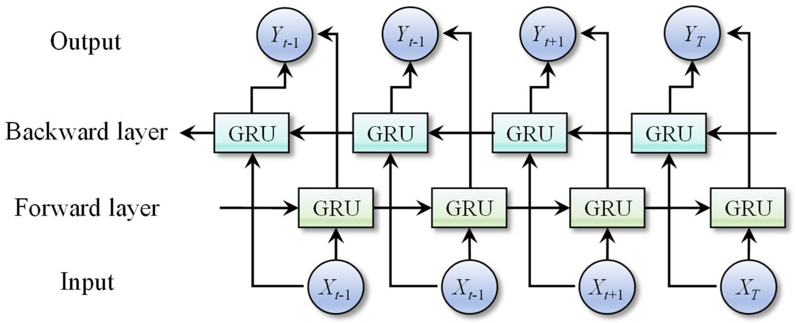
3.3. Bidirectional Gated Recurrent Unit

The gated recurrent unit (GRU) represents a variant of long short-term memory (LSTM) networks [38], featuring only reset and update gates with fewer parameters and faster convergence compared to LSTM. The internal information propagation within a GRU cell is given as follows:

$$\left\{\begin{array}{c}{r}_t=\sigma (W_x{x}_t+U_h{h}_{t-1}+b_r)\hfill \\ z_t=\sigma (W_z{x}_t+U_z{h}_{t-1}+b_z)\hfill \\ {\stackrel{-}{h}}_t=\mathit{tan}h(W_h{x}_t+U_h(r_t\odot h_t-1)+b_h)\hfill \\ h_t=(1-z_t)\odot h_{t-1}+z_t\odot {\stackrel{-}{h}}_t\hfill \end{array}\right.,$$

(8)

where $r_t$, $z_t$ denote the reset gate and update gate outputs, respectively; σ represents the sigmoid activation function; W and U are the weight matrices; $x_t$ is the input vector at time t; $h_{t-1}$ is the previous hidden state; b terms indicate the bias vectors; ${\stackrel{-}{h}}_t$, $h_t$ correspond to the candidate hidden state and final hidden state at time t; and tanh denotes the state activation function.

The bidirectional gated recurrent unit (BiGRU) is an improved variant of the standard GRU, which incorporates two parallel GRUs processing sequences in opposite directions. These two GRUs operate independently, with their outputs jointly controlling the final prediction. Compared to the unidirectional GRU, the BiGRU can more effectively capture temporal dependencies within monitoring data by simultaneously analyzing both forward and backward contexts. Consequently, the BiGRU model demonstrates superior predictive performance in time-series forecasting tasks. Figure 2 illustrates the architecture of the BiGRU network.

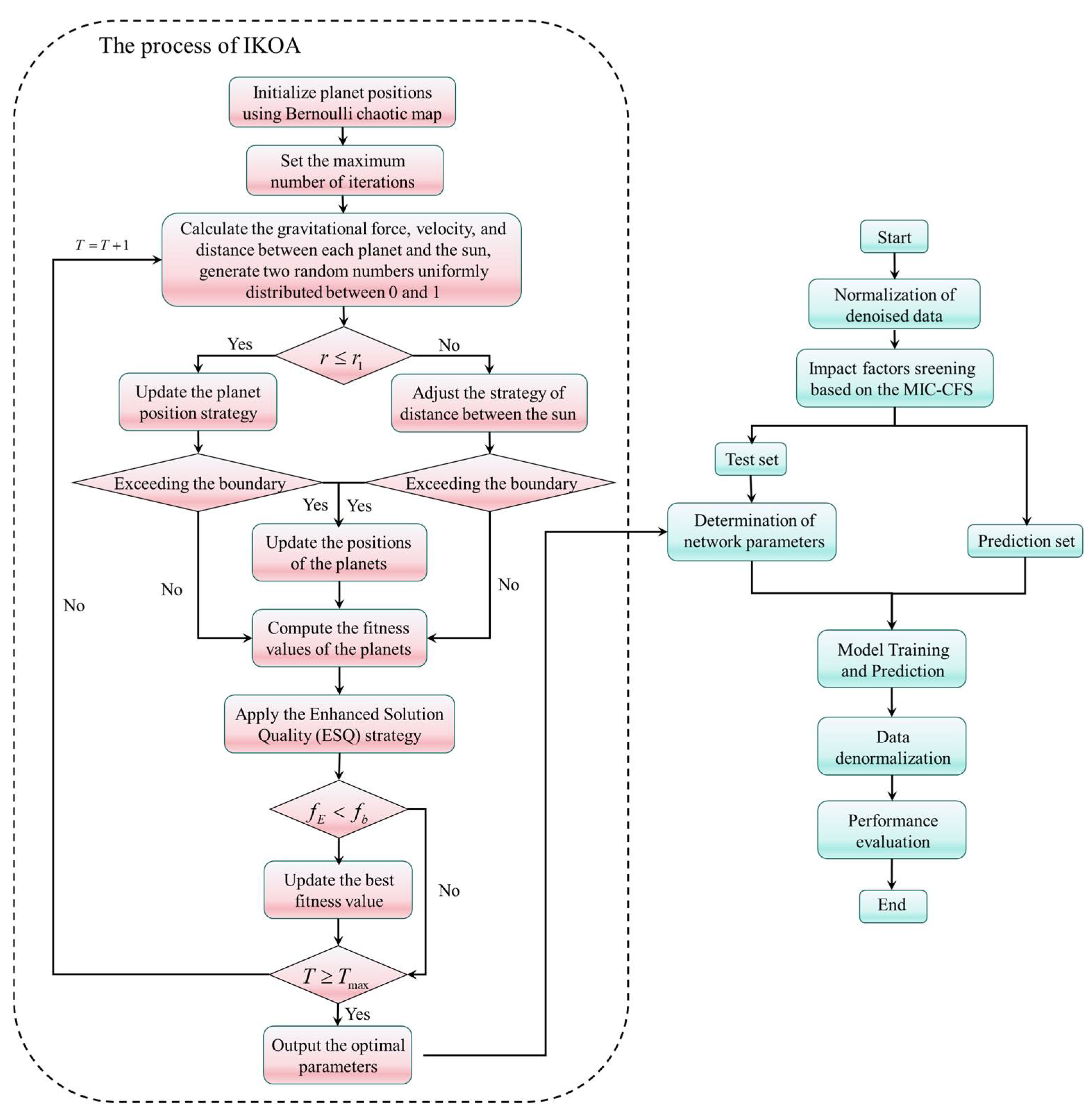
3.4. Improved Kepler Optimization Algorithm

The prediction accuracy of the BiGRU is highly sensitive to its numerous hyperparameters, necessitating intelligent optimization for automatic parameter tuning. While the conventional Kepler optimization algorithm (KOA) generates initial solutions randomly, resulting in non-uniform planetary distributions and frequent boundary violations. Hence, we propose a threefold enhancement: (1) Bernoulli chaotic mapping during initialization to maximize position diversity, (2) Runge–Kutta-based boundary handling for position updates, and (3) exponential sine quantization (ESQ) strategy to escape local optima and strengthen global search capability. This optimized framework systematically addresses the limitations of the KOA in hyperparameter optimization for the BiGRU architecture, and its principle is illustrated in Figure 3.

(1)

Bernoulli chaotic mapping

Bernoulli chaotic mapping is frequently employed for optimization algorithm initialization due to its uniform ergodicity and rapid convergence properties [39]:

$$z_{n+1}=\left\{\begin{array}{c}{z}_n/(1-\beta ),0\le z_n\le 1-\beta \hfill \\ (z_n-(1-\beta \left)\right)/\beta ,1-\beta \le z_n\le 1\hfill \end{array}\right.,$$

(9)

where β denotes the mapping parameter, β∈ [0, 1].

(2)

Runge–Kutta-inspired position update

To address boundary violation issues during planetary position updates, a stochastic relocation function used to reposition out-of-bound particles randomly within the search space is expressed as follows:

$$X_{i^{’}}=L_d+\mathrm{rand}(U_d-L_d),$$

(10)

where L_d and U_d represent the lower and upper bounds of the d-dimensional search space, respectively, with rand ∈ [0, 1] being a uniform random number.

Building upon the RUN optimization algorithm [40], the fourth-order Runge–Kutta method is applied to update the location of the planetary body. The equation is expressed as follows:

$$x_{\mathrm{new}1}=\left(X_{i^{’}}-\mathrm{rand}\cdot X_{i^{’}}\right)+SF\cdot \left(SM+\left(2\cdot \mathrm{rand}\cdot X_s-X_{i^{’}}\right)\right),$$

(11)

where SM (slope modifier) is determined through weighted averaging of four intermediate variables, mimicking solution dynamics in the search space, and SF (scaling factor) controls the movement magnitude of solutions.

The slope modifier is computed as follows:

$$SM=(k_1+2k_2+2k_3+k_4)/6,$$

(12)

where 1/6 is the standard Runge–Kutta weighting coefficient, and k₁, k₂, k₃, and k₄ are determined as follows:

$$\left\{\begin{array}{c}{k}_1=0.5\cdot (\mathrm{r}\mathrm{a}\mathrm{n}\mathrm{d}\cdot X_s-C\cdot X)\hfill \\ k_2=0.5\cdot (\mathrm{r}\mathrm{a}\mathrm{n}\mathrm{d}\cdot (X_s+q_2\cdot k_1\cdot \Delta x/2)-(C\cdot X_s+q_1\cdot k_1\cdot \Delta x/2\left)\right)\hfill \\ k_3=0.5\cdot (\mathrm{r}\mathrm{a}\mathrm{n}\mathrm{d}\cdot (X_s+q_2\cdot k_2\cdot \Delta x/2)-(C\cdot X_s+q_1\cdot k_2\cdot \Delta x/2\left)\right)\hfill \\ k_4=0.5\cdot (\mathrm{r}\mathrm{a}\mathrm{n}\mathrm{d}\cdot (X_s+q_2\cdot k_3\cdot \Delta x)-(C\cdot X_s+q_1\cdot k_3\cdot \Delta x\left)\right)\hfill \end{array}\right.,$$

(13)

where Δx denotes the adaptive step size and C, q₁, and q₂ are the adjustment coefficients introducing stochasticity to simulate planetary dynamics.

The scaling factor incorporates an exponential decay mechanism:

$$SF=2\cdot (0.5-\mathrm{rand})\cdot f,$$

(14)

$$f=a\cdot \mathit{exp}\left(-b\cdot \mathrm{rand}\cdot (T/T_{max}()\right),$$

(15)

where T represents the current iteration count; T_max is the maximum iteration number; and a and b are the constants used to determine the initial size and the reduction rate of f, respectively.

(3)

ESQ exploration enhancement

The exponential sine quantization (ESQ) strategy dynamically adjusts the search behavior by synthesizing both exploration and exploitation states of planetary agents, significantly improving the algorithmic performance:

$$X_{\mathrm{new}3}=\left\{\begin{array}{c}{X}_{\mathrm{new}2}+r\cdot \omega \left|\left(X_{\mathrm{new}2}-X_{\mathrm{avg}}\right)+\mathrm{rand}\right| , \mathrm{i}\mathrm{f} \omega <1\hfill \\ X_{\mathrm{new}2}+\left|r\cdot \omega \cdot \left(u\cdot X_{\mathrm{new}2}-X_{\mathrm{avg}}\right)+\mathrm{rand}\right|, else\hfill \end{array}\right.,$$

(16)

where r∈{−1, 0, 1} is a random integer and u∈ [0, 2] denotes a uniform random number.

The adaptive weight coefficient ω follows an exponential decay:

$$\omega =\mathrm{rand}\left(\mathrm{0,2}\right)\cdot \mathit{exp}\left(-c(T/T_{\max })\right),$$

(17)

where c is a stochastic constant.

The reference position $X_{\mathrm{avg}}$ combines three random solutions:

$$X_{\mathrm{avg}}=(X_{r1}+X_{r2}+X_{r3})/3$$

(18)

The updated position blends exploration and exploitation as follows:

$$X_{\mathrm{new}2}=\beta \cdot X_{\mathrm{avg}}+(1-\beta )\cdot X_s,$$

(19)

where β is a random term, β∈ [0, 1].

Upon obtaining a new solution, a greedy selection strategy is employed. If the fitness value of the new solution is superior to (i.e., lower than) that of the current optimal solution, the reinforcement is considered successful and the solution is retained; otherwise, the reinforcement is discarded. In summary, the pseudocode representation of the IKOA-based hyperparameter optimization for the BiGRU is exhibited in

Table 1. Pseudocode of the IKOA for the BIGRU hyperparameter optimization.

Input:        - BIGRU hyperparameter search space H = {h₁, h₂,…, h_D}                e.g., h = [learning rate, number of neurons]        - f(h): Objective function        - N: Number of planets (population size)        - Tmax: Max number of iterations        - Bound: lower & upper bounds for each hyperparameter Output:        - h_best: Optimal hyperparameter set        - f(h_best): Best validation performance

1. Initialization with Bernoulli Chaotic Mapping:         for i in 1 to N:                 for each dimension d in H:                         β = rand() in [0, 1]                         if 0 <= z [i][d] <= 1−β:                                z[i][d] = z[i][d]/(1-β)                         else:                                z[i][d] = (z[i][d]-(1-β)/) 2. Evaluate fitness F[i] = f(P[i])       Set global_best = best P[i] with minimum F[i] 3. For T in 1 to Tmax:         a. For each planet i:                 i. Runge-Kutta Inspired Position Update Compute k1 =0.5*(rand() *f(P[i]))                       k2 = 0.5*(rand()*(f(P[i])+q2*k1*Δx/2 – (C* f(P[i])+q1*k1*Δx/2)                       k3 = 0.5*(rand()*(f(P[i])+q2*k2*Δx/2 – (C* f(P[i])+q1*k2*Δx/2)                       k4 =0.5*(rand()*(f(P[i])+q2*k3*Δx/2 – (C* f(P[i])+q1*k3*Δx/2)                       SM = (1/6) * (k1 + 2*k2 + 2*k3 + k4)                       f = a * exp(-b*rand()*T/Tmax)                       SF=2*(0.5-rand())*f                       New_P[i] = (f(P[i])-rand()*f(P[i])) + SF *(SM+2*rand()*f(P[i])- f(P[i]))                       If New_P[i] violates bounds:                                Relocate with stochastic repositioning:                                         New_P[i][d] = Lower[d] + rand() * (Upper[d] - Lower[d])                  ii. Apply ESQ strategy:                      r ∈ {−1, 0, 1}, u ∈ [0, 2], β ∈ [0, 1]                      ReferencePosition = (P[r1] + P[r2] + P[r3])/3                      ω = rand(0,2)*exp(-c*T/Tmax)                      ESQ_Position_temp=β* ReferencePosition+(1-β)* f(P[i])                     If ω < 1:                             ESQ_Position = ESQ_Position_temp+r*ω*|(ESQ_Position_temp- Ref erencePosition) + rand()|                       else:                             ESQ_Position = ESQ_Position_temp+ | r*ω* (u* ESQ_Position_temp- Ref erencePosition) + rand()|                       Evaluate f(ESQ_Position)                       If f(ESQ_Position) < f(P[i]):                               P[i] = ESQ_Position                iii. Evaluate New fitness F[i] = f(P[i])          b. Update global_best if new best found 4. Return global_best, f(global_best)

.

3.5. Establishment Steps of the Proposed Prediction Model

Establishment steps of the proposed prediction model are exhibited as follows:

Step 1: Data preprocessing.

Raw monitoring data typically contain significant noise, and large-span monitoring data may degrade the model’s prediction performance. Therefore, we first denoised the original monitoring data; then, we normalized the processed data and divided them into the training and testing sets.

Step 2: Impact factor screening.

Based on the statistical model of sluice seepage, the MIC–CFS method was introduced to select the primary impact factors of seepage behavior.

Step 3: Parameter initialization.

The root mean square error (RMSE) during model training served as the objective function for the IKOA algorithm.

Step 4: Model optimization and validation.

The normalized training data were fed into both the target BiGRU model and the comparative models. The positions of planets were initialized using the Bernoulli chaotic map. The worst and best fitness values of the current planets were computed, and the planet with the best fitness was designated as the sun. Subsequently, the distances and velocities between the planets and the sun were updated. According to the random selection mechanism, either the planet position update strategy or the adjustment strategy based on the distance to the sun was applied. If a planet moved beyond the boundary, it was repositioned randomly within the search space, and its position was updated according to Equation (10). The ESQ enhancement strategy was then executed. If the fitness value after enhancement surpassed the current best fitness, the enhancement was retained; otherwise, it was discarded.

After employing the IKOA algorithm to optimize the BiGRU parameters and output the optimal configuration, the normalized testing data were input into the optimized BiGRU model and the comparative models. Finally, the prediction results from all the models were denormalized to obtain final predictions.

Step 5: Prediction evaluation.

After obtaining the final prediction results from all the models, we analyzed the prediction performance of both the proposed model and the comparative models in this study. The flowchart of the establishment of the prediction model is represented in Figure 4.

4. Case Study

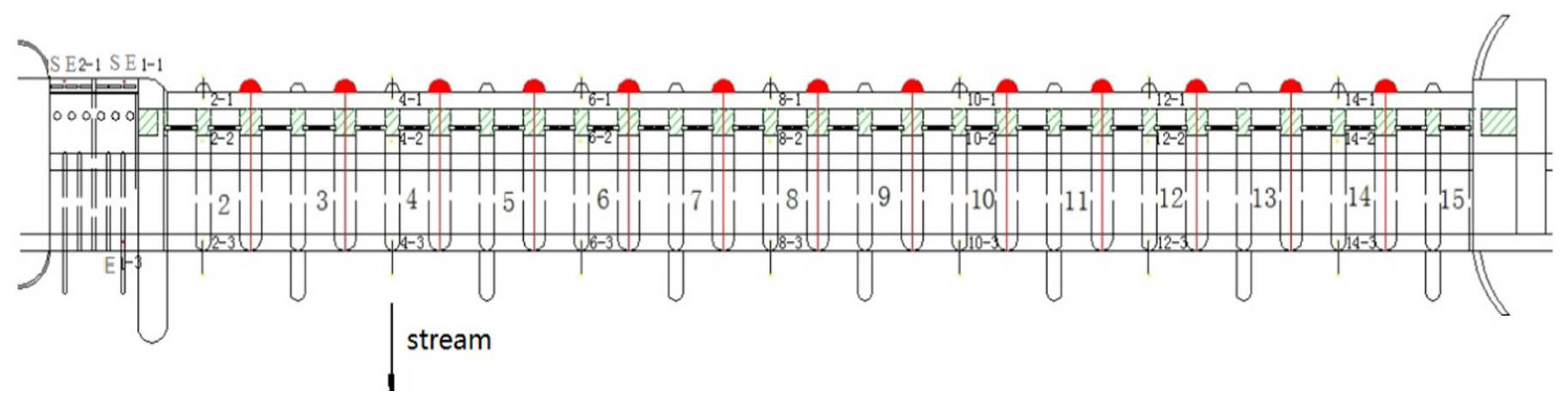
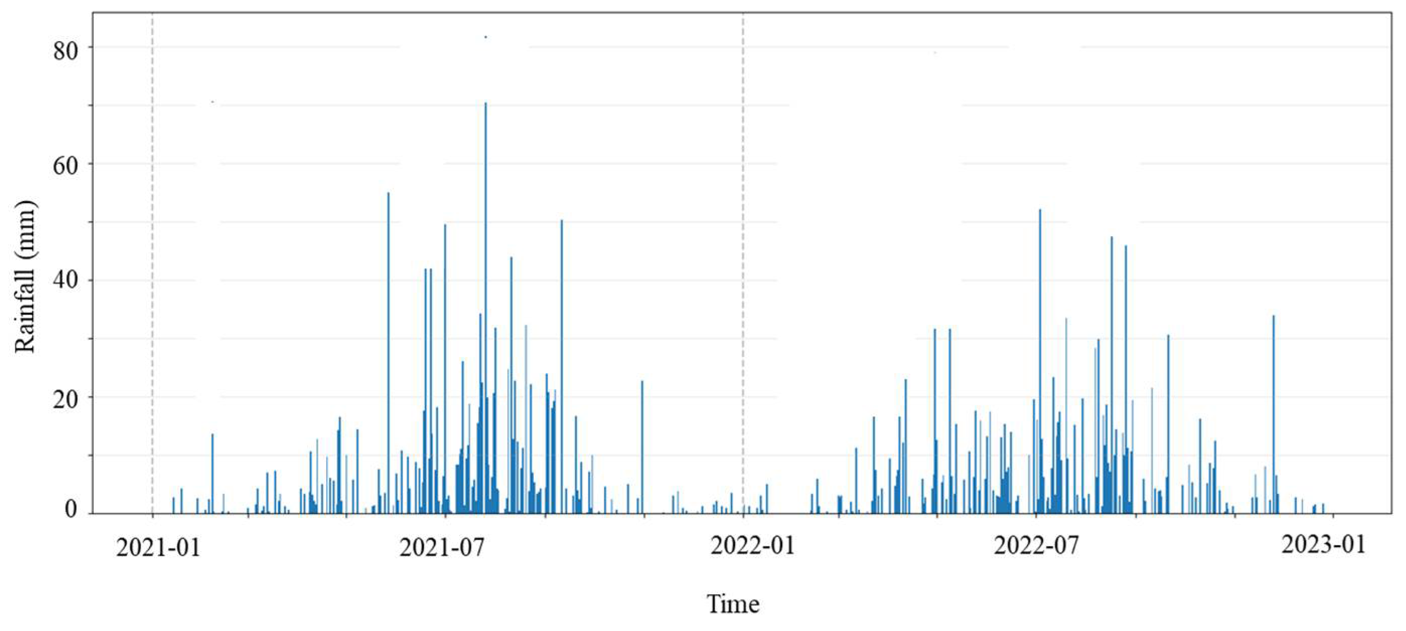
4.1. Project Overview

The Bengbu sluice project is located on the middle reaches of the Huai River, spanning the Huaishang and Yuhui districts of Bengbu City, approximately 250 km upstream from Hongze Lake. With a catchment area of 121,000 km² upstream of the sluice, the project consists of the 12-bay regulation sluice, the hydropower station, the navigation lock, and the flood diversion channel. The Bengbu sluice project serves multiple functions, including flood control, water storage for irrigation, navigation, power generation, and urban water supply, and it is a large-scale water control hub, as shown in Figure 5.

This study employs monitoring data from the Bengbu sluice project for analysis, specifically utilizing 72 sets of seepage measurements collected between 2021 and 2022. The dataset is divided into the training set (from January 2021 to June 2022, a total of 165 data points) and the test set (from June 2022 to December 2022, a total of 55 data points), with the latter period notably including July and August (the local flood season characterized by the maximum annual rainfall), during which the monitoring seepage data are incorporated into the model as rainfall characteristics.

The spatial arrangement of pressure monitoring tubes is illustrated in Figure 6. In this case, the typical monitoring points we selected were three monitoring points located at the left end, right end, and middle section of the sluice. The monitoring series of seepage and rainfall are shown in Figure 7 and Figure 8, respectively.

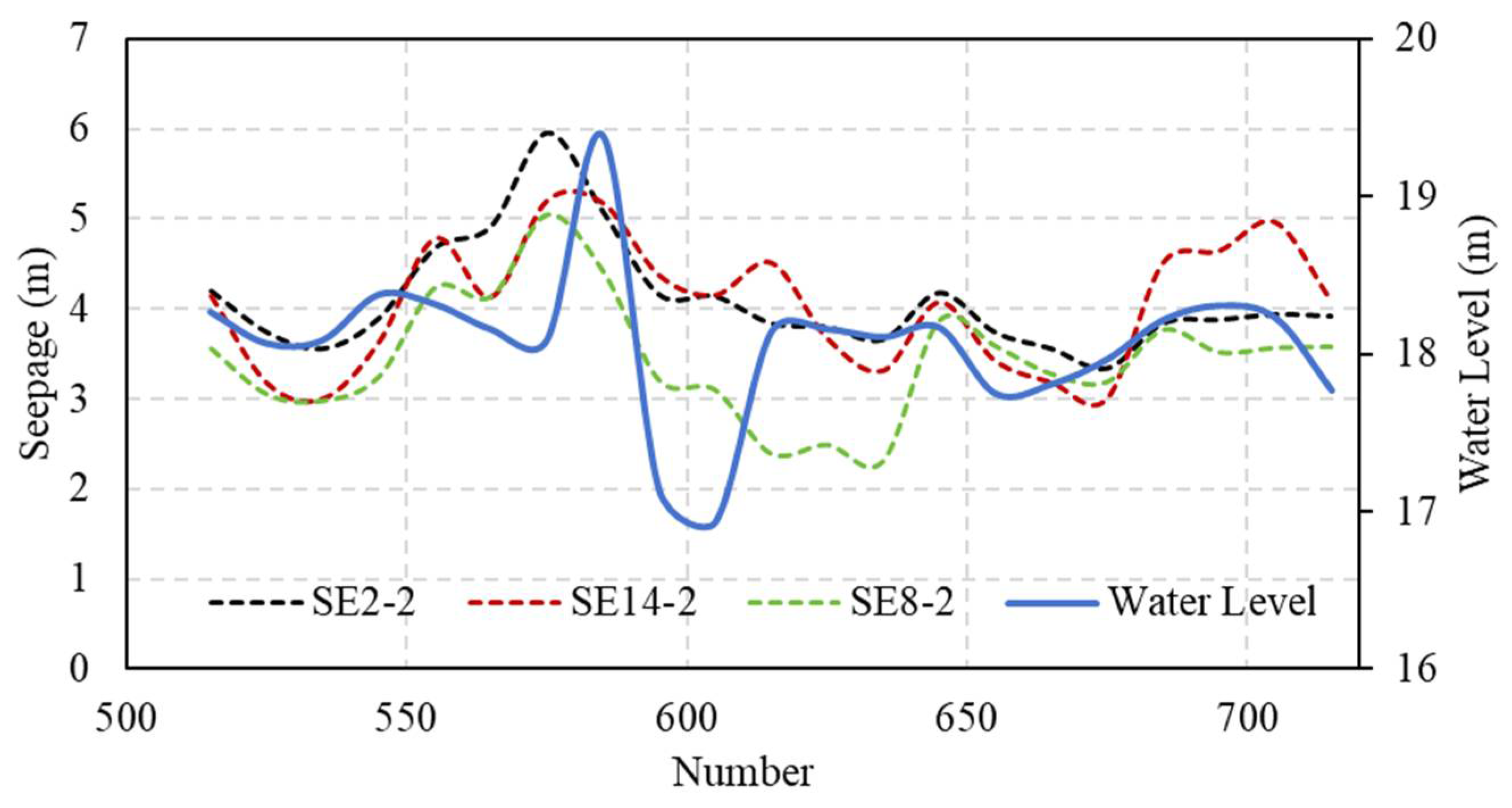
4.2. Results and Discussion

To demonstrate the effectiveness of the proposed model, this study establishes an impact factors screening and the IKOA–BiGRU-based model for predicting seepage at the Bengbu Sluice, with comparative analysis conducted against three alternative models (stepwise regression model, LSTM model, and GRU model) to evaluate predictive performance.

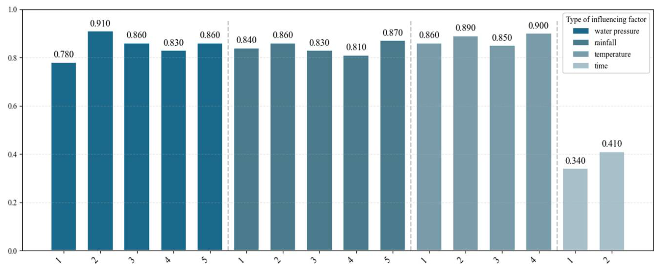
4.2.1. Impact Factor Screening Results

Previous studies demonstrated the superiority of the maximal information coefficient (MIC) algorithm over the Pearson correlation coefficient in detecting nonlinear relationships between variables through the construction of various function types. We further validated the MIC’s capability in identifying nonlinear dependencies using computational results from engineering case studies. According to Equation (6), the seepage exhibits dependence on 16 influencing factors, encompassing water level, rainfall, and their antecedent terms, as well as temperature and time effect.

Table 2. Comparison of correlation recognition capabilities between the Pearson correlation coefficient and the MIC.

Coefficient		MIC	Pearson
Impact factors about water pressure	$x_1$	0.84	0.95
	$x_2$	0.98	0.89
	$x_3$	0.94	0.92
	$x_4$	0.85	0.87
	$x_5$	0.81	0.84
Impact factors about rainfall	$x_6$	0.83	0.81
	$x_7$	0.73	0.44
	$x_8$	0.74	0.43
	$x_9$	0.77	0.58
	$x_{10}$	0.75	0.69
Impact factors about temperature	$x_{11}$	0.68	−0.23
	$x_{12}$	0.63	0.27
	$x_{13}$	0.72	0.33
	$x_{14}$	0.63	−0.43
Impact factors about time	$x_{15}$	0.44	0.06
	$x_{16}$	0.44	0.21

presents both Pearson correlation coefficient and MIC between seepage and various influencing factors.

As shown in Table 2, both methods effectively identify impact factors with strong linear correlations to sluice seepage, such as water pressure factors X1–X5 and rainfall factors X6–X10. However, the correlation coefficients between sluice seepage and temperature factors X11–X14 or aging factors X15–X16 reveal that Pearson’s method fails to detect nonlinear relationships. Consequently, this study adopts MIC-derived correlation coefficients as the metric for evaluating inter-variable relationships, as illustrated in Figure 9 and Figure 10.

Figure 9 presents the correlation heatmaps of seepage-related impact factors for monitoring points SE2-2 and SE14-2, respectively. As illustrated in Figure 9, significant correlations exist among the impact factors, while their correlation degrees with sluice seepage vary considerably. Specifically, strong inter-correlations are observed among water pressure factors X1–X5 (varying from 0.80 to 1.00) and rainfall factors X6–X10 (varying from 0.70 to 0.90), both of which exhibit substantial influence on sluice seepage. In contrast, temperature factors X11–X14 (varying from 0.60 to 0.70) and time effect factors X15–X16 (varying from 0.40 to 0.60) demonstrate relatively heterogeneous correlation patterns.

Figure 10 exhibits the correlation heatmaps of seepage-related impact factors for SE8-2. Consistent with theoretical expectations, sluice seepage shows a statistically significant correlation with both water pressure and rainfall impact factors. Notably, the correlation between temperature and sluice seepage displays moderate-to-strong positive relationships (varying from 0.84 to 0.89), while time effect factors exhibit a dynamic correlation at a range of 0.33~0.40.

Directly incorporating all impact factors as input features would inevitably introduce information redundancy and increase model complexity. Therefore, it is imperative to employ the MIC–CFS feature selection method to screen the previously constructed impact factors, thereby eliminating redundant variables and those with weak correlations while retaining factors strongly associated with sluice seepage.

Considering the differential influences of water pressure, rainfall, temperature, and time effect factors on sluice seepage, calculating CFS values for all possible feature subsets would incur prohibitive computational costs. To address this, our methodology involves (1) ranking all impact factors in descending order of their correlation coefficients with sluice seepage and (2) sequentially introducing factors into the feature subset starting from the highest-correlated one. This iterative process continues until the CFS value reaches its maximum, ensuring optimal feature selection while maintaining computational efficiency.

Following the aforementioned methodology, the water pressure, rainfall, temperature, and time effect impact factors were systematically screened. Figure 11 displays the CFS values for all influencing factor subsets of monitoring points SE2-2 and SE14-2, while Figure 12 presents the corresponding CFS values for SE8-2.

Figure 11 and Figure 12 demonstrate that water level and precipitation exert significant influences on seepage pressure at monitoring points SE2-2 and SE14-2, while SE8-2 exhibits additional pronounced temperature effects. From a mechanical perspective, seepage behavior at slope-proximal monitoring points (SE2-2/SE14-2) primarily reflects the soil mass’s hydraulic interaction, while the centrally located monitoring point (SE8-2) shows stronger thermal correlations due to crack-induced seepage pathways in the dam foundation and sluice floor.

Through a rigorous selection process based on CFS, impact factors X2, X3, X4, X6, X7, X10, X12, and X15 for SE2-2; X2, X3, X4, X6, X7, X8, X11, and X15 for SE14-2; and X2, X3, X5, X6, X7, X8, X12, X14, and X16 for SE8-2 were ultimately identified as the optimal input features for the IKOA–BiGRU prediction model, based on their superior correlation characteristics and minimal information redundancy.

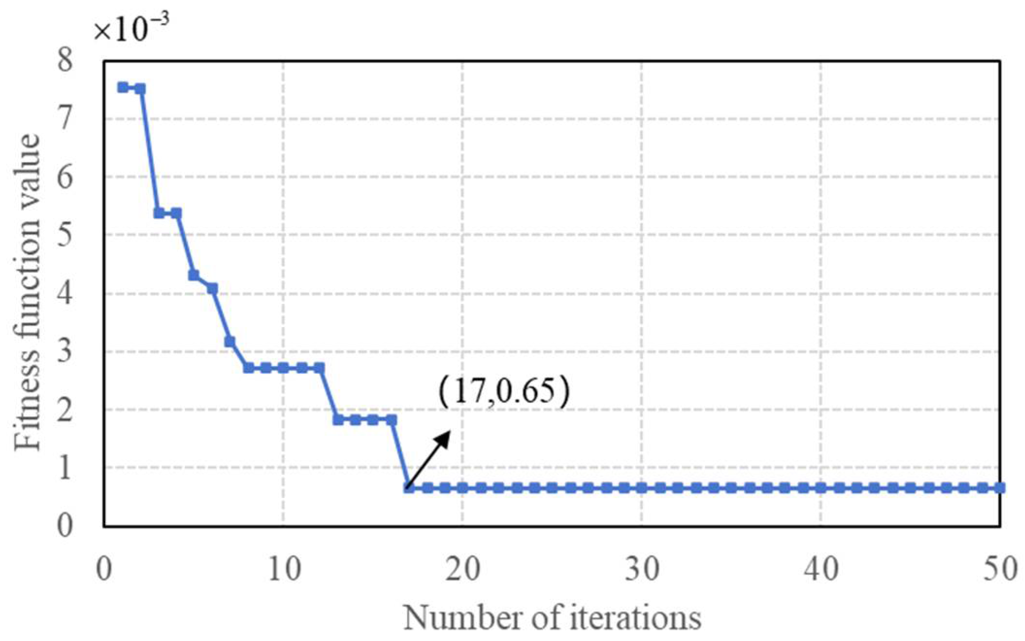
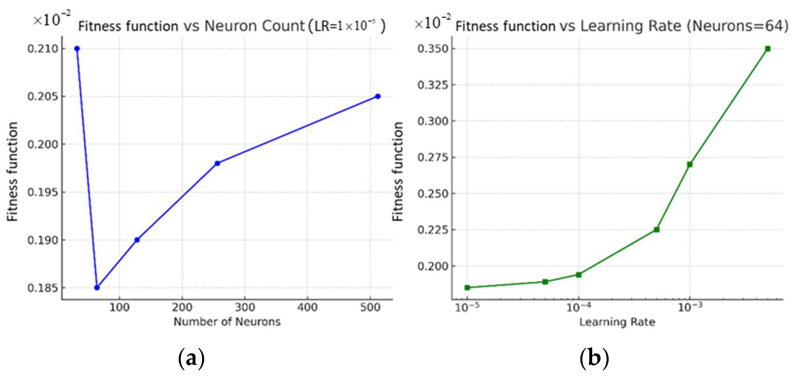
4.2.2. Results of the IKOA–BIGRU Model

Based on the identified impact factors in Section 4.2.1, we subsequently developed the sluice seepage prediction model. As presented in Section 3, the proposed approach utilizes the IKOA to optimize the hyperparameters of the BiGRU network, with the optimization objective set to minimize the training set’s root mean square error (RMSE). Considering the commonly used configurations in artificial neural network models for time-series and sequence modeling tasks, the key hyperparameters subject to optimization include the number of neurons (search range: 32–256) and the learning rate (search range: 1 × 10⁻⁵–1 × 10⁻³). The IKOA algorithm terminates when either 50 iterations are completed or the optimization error converges below 1 × 10⁻³.

In Figure 13, it indicates that through this optimization process, the fitness function converges at the 17^th generation, and at this time, the final BiGRU model architecture is determined to consist of 64 neurons with a learning rate of 1 × 10⁻⁵.

To evaluate the sensitivity of the BiGRU model to its key hyperparameters, we conducted a localized test by varying one parameter while fixing the other. The results in Figure 14 indicate that the values of the fitness function remained relatively stable when the number of neurons was within the range of 64–128, while the learning rate had a more pronounced effect: rates above 1 × 10⁻³ caused divergence, and those below 1 × 10⁻⁵ led to slow convergence. These results support the choice of 64 neurons and a learning rate of 1 × 10⁻⁵, including as a balanced configuration in terms of model complexity, convergence behavior, and generalization performance.

Based on the determined hyperparameters, the proposed sluice seepage prediction model was constructed. Figure 15 exhibits the fitting and predicting results for SE2-2, SE14-2, and SE8-2 based on the proposed model. It is noted that the modeled data series fitted the monitoring data very well, and the prediction results demonstrated satisfactory agreement with the actual monitoring data as well.

4.2.3. Model Interpretability Analysis Through SHAP

The proposed improved IKOA–BiGRU seepage prediction model demonstrates strong capability in modeling complex nonlinear relationships within time-series monitoring data and their influencing factors. However, its inherent lack of interpretability presents a significant limitation for engineering analysis and decision-making applications. To address this challenge, we employed SHapley Additive exPlanations (SHAP) to quantitatively evaluate factor influences on seepage in sluices. This approach adopts an additive feature attribution strategy that decomposes the proposed model output into constituent factor contributions, expressed as follows:

$$g(z)={\varphi }_0+{\sum }_{i=1}^m{\varphi }_i{z}_i,$$

(20)

where g(z) represents the explanatory model approximating the output of the proposed model $\widehat{f}\left(x\right)$, m denotes the number of input factors, z∈{0,1}^m indicates whether the factor is present ($z_i$ = 1) or absent ($z_i$ = 0), ${\varphi }_0$ represents the constant term of the explanatory model, ${\varphi }_i$ quantifies the Shapley value contribution of factor x_i to $\widehat{f}\left(x\right)$. The calculation of the Shapley value ${\varphi }_i$ is rooted in the cooperative game theory, and the expression is as follows:

$${\varphi }_i={\sum }_{S\subseteq \{x_1,x_2,\dots ,x_m\}\setminus \left\{x_i\right\}}{\displaystyle \frac{\left|S\right|!(m-|S|-1)!}{m!}}\left[\widehat{f}(S\cup \{x_i\})-\widehat{f}(S)\right],$$

(21)

where S represents a subset of variable combinations from the complete feature set, {x₁,x₂,…,xₘ}/{xᵢ} denotes the set of all variables excluding xᵢ, and $\widehat{f}(S)$ indicates the output prediction of the proposed model when using only the variable subset S.

The Shapley value determined based on Equation (21) employs an approach to objectively quantify the importance of variables that constitute the model and averages the marginal contribution $\widehat{f}(S\cup \{x_i\})-\widehat{f}(S)$ of the variable x_i. The Shapley value is computed for individual predictions and reflects the local importance of a specific variable. The global importance of the variable x_i is then obtained by aggregating its local contributions over the training set, and the expression is represented as:

$$I_i={\displaystyle \frac{{\sum }_{j=1}^N| {\varphi }_i^{\left(j\right)}|}{{\sum }_{l=1}^m{\sum }_{j=1}^N| {\varphi }_l^{\left(j\right)}|}},$$

(22)

where ${\varphi }_i^{\left(j\right)}$ represents the local importance of factor x_i for the j^th monitoring data.

In this case, 100 samples were randomly selected from the training dataset, and the Shapley values of each input variable were computed (Equation (21)). The resulting feature contributions are visualized in Figure 16, where each data point represents the Shapley value of a specific feature for an individual sample. In Figure 16, the horizontal axis indicates both the magnitude and direction of each feature’s contribution to seepage predictions, while the vertical axis organizes features according to their global importance ranking. A color gradient from red to blue corresponds to normalized feature values, enabling simultaneous interpretation of value ranges and their predictive impacts.

Figure 17 presents the aggregated global importance of each variable, calculated as the mean absolute Shapley value across all the samples (Equation (22)). The combined interpretation of both figures demonstrates consistent identification of dominant impact factors for sluice seepage across monitoring points. The analysis confirms that water pressure variation constitutes the most significant driver of sluice seepage, followed by rainfall-related terms. These findings validate the model’s ability to capture physically meaningful relationships while maintaining computational robustness.

The SHAP value distribution reveals distinct patterns in factor contributions to sluice seepage. Positive Shapley values (red) are predominantly associated with water level elevation, indicating its direct positive correlation with seepage. This finding aligns with fundamental structural mechanics principles where increased hydrostatic pressure induces seepage.

For the impact factors related to rainfall, the positive Shapley values also account for a substantial proportion, mostly distributed within the range of 0–3. The results indicate the positive correlation with seepage as well, which aligns with physical principles, namely, that rainfall-induced water level rise intensifies seepage.

Regarding the impact factors related to temperature and time effects, the selected factors exhibit positive correlations with seepage, but relatively weak compared to impact factors related to water level and rainfall.

The alignment between the SHAP-derived importance attributions and the well-established physical principles of sluice behavior strongly supports the model’s ability to capture the underlying physics of seepage variations. Moreover, the model effectively replicates the magnitude of the key influencing factors.

4.2.4. Fitting and Prediction Results Comparison

To validate the effectiveness of fitting and prediction capability of the proposed model, we systematically evaluated its performance through comparative analysis with three benchmark models: the stepwise regression model, the IKOA–LSTM model, and the IKOA–GRU model.

The performance of time series prediction models requires both qualitative and quantitative assessment. While visual inspection of prediction-standard data comparisons provides intuitive subjective evaluation, objective metric-based analysis is essential for rigorous scientific validation. This study employs six evaluation metrics with distinct mathematical formulations:

Metric 1: mean absolute error (MAE).

Quantifies the average magnitude of the absolute prediction errors:

$$MAE={\displaystyle \frac{1}{m}}{\sum }_{i=1}^m\left|y_{test,i}-{\widehat{y}}_{test,i}\right|,$$

(23)

where m represents the sample size, ytest, i denotes the measured values, and ${\widehat{y}}_{test,i}$ indicates the predicted values.

Metric 2: mean square error (MSE).

Measures the average squared deviation between the predictions and the observations, emphasizing larger errors:

$$MSE={\displaystyle \frac{1}{m}}\sum _{i=1}^m{\left(y_{test,i}-{\widehat{y}}_{test,i}\right)}^2$$

(24)

Metric 3: root mean square error (RMSE).

Provides error magnitude in original units through square root transformation:

$$RMSE=\sqrt{{\displaystyle \frac{1}{m}}\sum _{i=1}^m{\left(y_{test,i}-{\widehat{y}}_{test,i}\right)}^2}$$

(25)

Metric 4: coefficient of determination (R²).

Evaluates the proportion of variance explained by the model, with values bounded at [0, 1]:

$$R^2=1-{\displaystyle \frac{{\sum }_{i=1}^m{(y_{test,i}-{\widehat{y}}_{test,i})}^2}{{\sum }_{i=1}^m{(y_{test,i}-{\stackrel{-}{y}}_{test})}^2}},$$

(26)

where ${\stackrel{-}{y}}_{test}$ signifies the mean of the observed values. Model accuracy increases as R² approaches unity.

Metric 5: Willmott index (WI).

Evaluates the consistency between the predictions and the observations, which is mathematically expressed as follows:

$$WI=1-{\displaystyle \frac{{\sum }_{i=1}^n({\widehat{y}}_{test,i}-y_{test,i}{)}^2}{{\sum }_{i=1}^n{\left(|{\widehat{y}}_{test,i}-{\stackrel{-}{y}}_{test}|+|y_{test,i}-{\stackrel{-}{y}}_{test}|\right)}^2}}$$

(27)

Metric 6: Kling–Gupta efficiency (KGE).

Evaluates the accuracy of the prediction model, which includes components of correlation, bias, and variability, and the expression is as follows:

$$KGE=1-\sqrt{(r-1{)}^2+(\alpha -1{)}^2+(\beta -1{)}^2},$$

(28)

where $r$ denotes the Pearson correlation coefficient between the predicted and observed values; $\alpha$ denotes the variability ratio, $\alpha ={\displaystyle \frac{{\sigma }_p}{{\sigma }_o}}$, ${\sigma }_p$, and ${\sigma }_o$ represent the standard deviations of the predicted and observed values, respectively; $\beta$ denotes the bias ratio, which is determined as $\beta ={\displaystyle \frac{{\mu }_p}{{\mu }_o}}$; and ${\mu }_p$ and ${\mu }_o$ denote the means of the predicted and observed values.

Figure 16 represents the results of fitting, predicting, and corresponding residuals of the four models. As evidenced in Figure 18, the proposed method demonstrates superior performance relative to the three comparative models, exhibiting both a lower mean absolute error (0.057 for SE2-2, 0.064 for SE14-2, and 0.074 for SE8-2) and a significantly reduced error variability (variation amplitude of 0.16, 0.12, and 0.39 for SE2-2, SE14-2, and SE8-2, respectively). The results demonstrate that the stepwise regression model underperforms as compared to the other three models in both fitting and predicting performance, indicating that the structural behavior of sluice seepage exhibits complex nonlinear interactions with external environmental factors. The IKOA–LSTM and IKOA–GRU models exhibit strong capabilities in characterizing nonlinear relationships, with minimal discrepancies between modeled and monitored values. To evaluate the interpretability and the prediction capability of these four models, six evaluation metrics were established, and the results are listed in

Table 3. The results of the evaluation metrics of the proposed model, the stepwise regression model, the IKOA–LSTM model, and the IKOA–GRU model.

Evaluation Metric		IKOA–BiGRU Model	Stepwise Regression Model	IKOA–LSTM Model	IKOA–GRU Model
SE2-2	MAE	0.0567	0.3005	0.1348	0.1319
	MSE	0.0051	0.1123	0.0254	0.0239
	RMSE	0.0709	0.3282	0.1579	0.1531
	R2	0.9853	0.5896	0.9183	0.9321
	WI	0.9595	0.7473	0.8984	0.9058
	KGE	0.9659	0.7941	0.9245	0.9117
SE8-2	MAE	0.0638	0.09	0.0643	0.0795
	MSE	0.0054	0.0124	0.0063	0.0082
	RMSE	0.0729	0.1112	0.0776	0.0882
	R2	0.9879	0.9721	0.9844	0.9805
	WI	0.9636	0.9481	0.9612	0.9532
	KGE	0.9749	0.9544	0.9645	0.9665
SE14-2	MAE	0.0743	0.1138	0.1014	0.0986
	MSE	0.0124	0.0186	0.0214	0.0181
	RMSE	0.1112	0.1317	0.1335	0.1346
	R2	0.9736	0.9587	0.9514	0.9597
	WI	0.9601	0.9379	0.9438	0.9461
	KGE	0.9655	0.9476	0.9546	0.9498

.

According to the results of the evaluation metrics of each model presented in Table 3, the proposed model achieves remarkable error minimization, with average MAE (0.0649), MSE (0.0076) and RMSE (0.0850) values lower than those of the closest competitor (IKOA–LSTM: average MAE = 0.1001, MSE = 0.0177, RMSE = 0.1230). This improvement in prediction accuracy suggests the model effectively seizes complex temporal structures and bidirectional dependencies, which eventually improve the predictive accuracy.

Based on the results of evaluation metrics of R², WI, and KGE, all the models show acceptable performance for SE8-2 and SE14-2, as the R², WI, and KGE values of all the four models exceeded 0.95, 0.93, and 0.94, respectively. Similarly, the proposed model uniquely excels in advanced indicators, R² (0.9736–0.9879 vs. 0.5896–0.9844 for the other models), WI (0.9595–0.9636 vs. 0.7473–0.9612 for the other models), and KGE (0.9655–0.9749 vs. 0.7941–0.9665 for the other models), which verifies the superior model interpretability and consistency compared to the other three models.

In conclusion, compared with the other benchmark models, the proposed seepage prediction model demonstrates better predictive performance, which is expected to provide a more effective solution for monitoring and forecasting seepage in hydraulic engineering applications.

5. Conclusions

In order to accurately analyze and evaluate the seepage safety state of a sluice, in this study, a novel seepage prediction method based on the BiGRU model optimized by the IKOA is proposed, with key impact factors selected through a rigorous screening process. The main conclusions can be drawn as follows:

(1)

The main impact factor screening method based on the MIC–CFS effectively identifies a set of features with high relevance to sluice seepage and low redundancy. The process of the selection reduces the complexity of the prediction model significantly, mitigates the risk of overfitting, and enhances the overall generalization and prediction accuracy.

(2)

By optimizing the Kepler optimization algorithm (KOA) based on chaotic mapping, Runge–Kutta position updating, and ESQ strategies, the efficiency of the optimization algorithm is significantly improved. The integration of the improved Kepler optimization algorithm (IKOA) for hyperparameter tuning effectively reduces the uncertainty associated with manual parameter selection, improving the efficiency of model development as a result.

(3)

The case study demonstrates that, compared to other predictive models, the IKOA–BiGRU model exhibits obvious advantages in sluice seepage prediction. Incorporating the BiGRU model into the prediction framework effectively compensates for the limitations of the GRU in capturing deep temporal features of sluice seepage data, enabling a more accurate representation of seepage patterns. The proposed model demonstrates superior prediction performance, with R² values ranging from 0.974 to 0.988 and MAE values between 0.074 and 0.064. Comparative analyses further vali-date the effectiveness and feasibility of the proposed model, highlighting its potential as a valuable reference for practical sluice seepage forecasting.

Nevertheless, our study primarily focuses solely on seepage at a single monitoring point of a sluice, which limits the spatial comprehensiveness of the model. In practical engineering applications, seepage behavior exhibits spatiotemporal correlations across multiple locations within a sluice structure. In future work, it is necessary to incorporate multi-point monitoring data to capture spatial interactions and coupling effects among different regions of the sluice structure. By incorporating multi-point seepage monitoring sequences, a more comprehensive multi-point seepage prediction model for sluices can be developed to further enhance prediction accuracy and reliability. Furthermore, future studies may also explore real-time data fusion techniques and uncertainty quantification methods to enhance model adaptability under varying environmental conditions.

References

1. Fan, X.; Wu, Z.; Liu, L.; Wen, Y.; Yu, S.; Zhao, Z.; Li, Z. Analysis of Sluice Foundation Seepage Using Monitoring Data and Numerical Simulation. Adv. Civ. Eng. 2019, 2019, 2850916. [Google Scholar]
2. Zhang, T.; Li, C.; Du, X.; Yu, Y. Anti-seepage Technology for a Sluice Foundation on Soft Soil. Appl. Mech. Mater. 2014, 638, 384–388. [Google Scholar]
3. Ma, F.; Hu, J.; Ye, W. Study on key technical elements of technical specification for sluice safety monitoring. Water Resour. Hydropower Eng. 2019, 50, 90–94. (In Chinese) [Google Scholar]
4. Chen, S. Sluices and barrages. In Hydraulic Structures; Springer: Berlin/Heidelberg, Germany, 2015; pp. 643–713. [Google Scholar]
5. Huang, Z.; Gu, C.; Peng, J.; Wu, Y.; Gu, H.; Shao, C.; Zheng, S.; Zhu, M. A Statistical Prediction Model for Sluice Seepage Based on MHHO-BiLSTM. Water 2024, 16, 191. [Google Scholar] [CrossRef]
6. Cai, X.; Cui, Z.; Guo, X.; Li, F.; Zhang, Y. Seismic Safety Design and Analysis of Hydraulic Sluice Chamber Structure Based on Finite Element Method. Comput. Intell. Neurosci. 2022, 2022, 6183588. [Google Scholar] [CrossRef]
7. Chen, L. Safety Monitoring of Sluice Gate of Xinglong Water Control Project on Hanjiang River. Rural. Water Conserv. Hydropower China 2015, 8, 165–167. [Google Scholar]
8. Liu, Y.; Luo, L.; Wu, G. Analysis and Study on Seepage Safety Monitoring of Zhaoshandu Diversion Project. In Proceedings of the 2022 8th ICHCE, Xi’an, China, 25–27 November 2022; pp. 1027–1031. [Google Scholar]
9. Yu, G.; Wang, Z.; Zhang, B.; Xie, Z. The grey relational analysis of sluice monitoring data. Procedia Eng. 2011, 15, 5192–5196. [Google Scholar]
10. Liu, B.; Cen, W.; Zheng, C.; Li, D.; Wang, L. A combined optimization prediction model for earth-rock dam seepage pressure using multi-machine learning fusion with decomposition data-driven. Expert Syst. Appl. 2024, 242, 122798. [Google Scholar] [CrossRef]
11. Fatehi-Nobarian, B.; Fard Moradinia, S. Wavelet–ANN hybrid model evaluation in seepage prediction in nonhomogeneous earthen dams. Water Pract. Technol. 2024, 19, 2492–2511. [Google Scholar] [CrossRef]
12. Rehamnia, I.; Al-Janabi, A.M.S.; Sammen, S.S.; Pham, B.T.; Prakash, I. Prediction of seepage flow through earthfill dams using machine learning models. HydroResearch 2024, 7, 131–139. [Google Scholar] [CrossRef]
13. Cao, W.; Wen, Z.; Feng, Y.; Zhang, S.; Su, H. A multi-point joint prediction model for high-arch dam deformation considering spatial and temporal correlation. Water 2024, 16, 1388. [Google Scholar] [CrossRef]
14. Shao, C.; Gu, C.; Yang, M.; Xu, Y.; Su, H. A novel model of dam displacement based on panel data. Struct. Control. Health Monit. 2018, 25, e2037. [Google Scholar] [CrossRef]
15. Cai, S.; Gao, H.; Zhang, J.; Peng, M. A self-attention-LSTM method for dam deformation prediction based on CEEMDAN optimization. Appl. Soft Comput. 2024, 159, 111615. [Google Scholar] [CrossRef]
16. Lei, W.; Wang, J. Dynamic Stacking ensemble monitoring model of dam displacement based on the feature selection with PCA-RF. J. Civ. Struct. Health Monit. 2022, 12, 557–578. [Google Scholar] [CrossRef]
17. Kang, X.; Li, Y.; Zhang, Y.; Wen, L.; Sun, X.; Wang, J. PCA-IEM-DARNN: An enhanced dual-stage deep learning prediction model for concrete dam deformation based on feature decomposition. Measurement 2025, 242, 115664. [Google Scholar] [CrossRef]
18. Deng, Y.; Zhang, D.; Cao, Z.; Liu, Y. Spatio-temporal water height prediction for dam break flows using deep learning. Ocean Eng. 2024, 302, 117567. [Google Scholar] [CrossRef]
19. Liu, Y.; Zheng, D.; Wu, X.; Chen, X.; Georgakis, C.; Qiu, J. Research on prediction of dam seepage and dual analysis of lag-sensitivity of influencing factors based on MIC optimizing random forest algorithm. KSCE J. Civ. Eng. 2023, 27, 508–520. [Google Scholar] [CrossRef]
20. Shi, Z.; Li, J.; Wang, Y.; Gu, C.; Jia, H.; Xu, N.; Pan, W. Characterization Model Research on Deformation of Arch Dam Based on Correlation Analysis Using Monitoring Data. Mathematics 2024, 12, 3110. [Google Scholar] [CrossRef]
21. Peng, J.; Xie, W.; Wu, Y.; Sun, X.; Zhang, C.; Gu, H.; Zhu, M.; Zheng, S. Prediction for the Sluice Deformation Based on SOA-LSTM-Weighted Markov Model. Water 2023, 15, 3724. [Google Scholar] [CrossRef]
22. Ma, Z.; Lou, B.; Shen, Z.; Ma, F.; Luo, X.; Ye, W.; Li, D. A Deformation Analysis Method for Sluice Structure Based on Panel Data. Water 2024, 16, 1287. [Google Scholar] [CrossRef]
23. Xing, Y.; Chen, Y.; Huang, S.; Wang, P.; Xiang, Y. Research on dam deformation prediction model based on optimized SVM. Processes 2022, 10, 1842. [Google Scholar] [CrossRef]
24. Xu, Y.; Bao, T.; Yuan, M.; Zhang, S. A Reservoir Dam Monitoring Technology Integrating Improved ABC Algorithm and SVM Algorithm. Water 2025, 17, 302. [Google Scholar] [CrossRef]
25. Jiang, Z. Monitoring model group of seepage behavior of earth-rock dam based on the mutual information and support vector machine algorithms. Struct. Health Monit. 2024, 24, 466–480. [Google Scholar] [CrossRef]
26. Zhang, Y.; Zhang, W.; Li, Y.; Wen, L.; Sun, X. AF-OS-ELM-MVE: A new online sequential extreme learning machine of dam safety monitoring model for structure deformation estimation. Adv. Eng. Inform. 2024, 60, 102345. [Google Scholar] [CrossRef]
27. Zhu, Y.; Yang, Z.; Huang, J. Intelligent Prediction on Cement Take of Dam Foundation Grouting Based on GOA-ELM Model. Hydraul. Struct. Hydrodyn. 2024, 608, 121–131. [Google Scholar]
28. Ou, B.; Zhang, C.; Xu, B.; Fu, S.; Liu, Z.; Wang, K. Innovative Approach to Dam Deformation Analysis: Integration of VMD, Fractal Theory, and WOA-DELM. Struct. Control Health Monit. 2024, 2024, 1710019. [Google Scholar] [CrossRef]
29. Al-Hardanee, O.F.; Demirel, H. Hydropower Station Status Prediction Using RNN and LSTM Algorithms for Fault Detection. Energies 2024, 17, 5599. [Google Scholar] [CrossRef]
30. Yang, X.; Xiang, Y.; Wang, Y.; Shen, G. A Dam Safety State Prediction and Analysis Method Based on EMD-SSA-LSTM. Water 2024, 16, 395. [Google Scholar] [CrossRef]
31. Hu, Y.; Gu, C.; Meng, Z.; Shao, C.; Min, Z. Prediction for the Settlement of Concrete Face Rockfill Dams Using Optimized LSTM Model via Correlated Monitoring Data. Water 2022, 14, 2157. [Google Scholar] [CrossRef]
32. Abdi, E.; Taghi Sattari, M.; Milewski, A.; Ibrahim, O.R. Advancements in Hydrological Modeling: The Role of bRNN-CNN-GRU in Predicting Dam Reservoir Inflow Patterns. Water 2025, 17, 1660. [Google Scholar] [CrossRef]
33. Hua, G.; Wang, S.; Xiao, M.; Hu, S. Research on the Uplift Pressure Prediction of Concrete Dams Based on the CNN-GRU Model. Water 2023, 15, 319. [Google Scholar] [CrossRef]
34. Xu, B.; Zhang, H.; Xia, H.; Song, D.; Zhu, Z.; Chen, Z.; Lu, J. A multi-level prediction model of concrete dam displacement considering time hysteresis and residual correction. Meas. Sci. Technol. 2024, 36, 015107. [Google Scholar] [CrossRef]
35. Ma, N.; Niu, X.; Chen, X.; Wei, W.; Zhang, Y.; Kang, X.; Wu, J. Analysis of Concrete Dam Deformation Prediction Based on the ResNet-GRU-SGWO Model. Adv. Civ. Eng. 2024, 2024, 4791788. [Google Scholar] [CrossRef]
36. Liu, W.; Wang, J.; Li, Z.; Lu, Q. ISSA optimized spatiotemporal prediction model of dissolved oxygen for marine ranching integrating DAM and Bi-GRU. Front. Mar. Sci. 2024, 11, 1473551. [Google Scholar] [CrossRef]
37. Reshef, D.; Reshef, Y.; Finucane, H.; Grossman, S.; McVean, G.; Turnbaugh, P.; Sabeti, P. Detecting novel associations in large data sets. Science 2011, 334, 1518–1524. [Google Scholar] [CrossRef]
38. Wu, T.; Wang, M.; Xi, Y.; Zhao, Z. Malicious URL Detection Model Based on Bidirectional Gated Recurrent Unit and Attention Mechanism. Appl. Sci. 2022, 12, 12367. [Google Scholar] [CrossRef]
39. Saito, A.; Yamaguchi, A. Pseudorandom number generation using chaotic true orbits of the Bernoulli map. Chaos Interdiscip. J. Nonlinear Sci. 2016, 26, 063122. [Google Scholar] [CrossRef]
40. Ahmadianfar, I.; Heidari, A.; Gandomi, A.; Chu, X.; Chen, H. RUN beyond the metaphor: An efficient optimization algorithm based on Runge Kutta method. Expert Syst. Appl. 2021, 181, 115079. [Google Scholar] [CrossRef]
Figure 1. Network architecture of an LSTM unit.
Water 17 01850 g001
Figure 2. Network architecture of the BiGRU.
Water 17 01850 g002
Figure 3. Improved Kepler optimization algorithm.
Water 17 01850 g003
Figure 4. Flowchart of the model establishment.
Water 17 01850 g004
Figure 5. Engineering overview of the 28-bay regulation sluice at Bengbu hydraulic project.
Water 17 01850 g005
Figure 6. Distribution of seepage monitoring points for the 28-bay regulation sluice at the Bengbu hydraulic project.
Water 17 01850 g006
Figure 7. Monitoring data series of seepage at three typical monitoring points and the corresponding water level.
Water 17 01850 g007
Figure 8. Monitoring data series of rainfall.
Water 17 01850 g008
Figure 9. Heatmaps of sluice seepage-related variables for monitoring points: (a) SE2-2 and (b) SE14-2.
Water 17 01850 g009
Figure 10. Heatmaps of sluice seepage-related variables for SE8-2.
Water 17 01850 g010
Figure 11. Bar chart of CFS values of impact factor subsets for monitoring points: (a) SE2-2 and (b) SE14-2.
Water 17 01850 g011
Figure 12. Bar chart of CFS values of impact factor subsets for SE8-2.
Water 17 01850 g012
Figure 13. The results of the fitness function across varying iterations.
Water 17 01850 g013
Figure 14. Sensitivity analysis of the BiGRU model with respect to two key hyperparameters: the number of neurons and the learning rate. (a) Values of the fitness function across varying neuron counts with the learning rate fixed at 1 × 10⁻⁵; (b) values of the fitness function across varying learning rates with the number of neurons fixed at 64.
Water 17 01850 g014
Figure 15. Fitting and predicting results of (a) SE2-2, (b) SE14-2, and (c) SE8-2.
Water 17 01850 g015
Figure 16. SHAP-based analysis of local feature importance and directional contributions for the sluice seepage prediction of (a) SE2-2, (b) SE8-2, and (c) SE14-2.
Water 17 01850 g016
Figure 17. Global importance ranking of input variables for sluice seepage prediction based on the Shapley values of (a) SE2-2, (b) SE8-2, and (c) SE14-2.
Water 17 01850 g017
Figure 18. Fitting and predicting results, residuals of the proposed model, the stepwise regression model, the IKOA–LSTM model, and the IKOA–GRU model for (a) SE2-2, (b) SE14-2, and (c) SE8-2.
Water 17 01850 g018