Abstract
The accurate prediction of wastewater quality parameters is pivotal for evaluating the treatment stability of processes and for ensuring regulatory compliance in wastewater treatment plants. A singular machine learning model often faces challenges in fully capturing and extracting the complex nonlinear relationships inherent in multivariate time series data. To overcome this limitation, this study proposes a dual hybrid modeling framework that effectively integrates LSTM and XGBoost models, leveraging their complementary strengths. The first hybrid model refines the residues to utilize the information, whereas the second hybrid model enhances the input features by extracting temporal dependencies. A comparative analysis against three standalone models reveals that the proposed hybrid framework consistently outperforms them in both predictive accuracy and generalization ability across four key effluent indicators—chemical oxygen demand, ammonia nitrogen, total nitrogen, and total phosphorus. These results demonstrate that the proposed hybrid machine learning framework has great potential to be used to evaluate process stability in wastewater treatment plants, paving a way for smarter, more resilient, and more sustainable wastewater management, which will improve ecological integrity and regulatory compliance.
1. Introduction
Water is essential for sustaining life, maintaining ecosystems, and supporting economic activities [1]. Water quality is critical for sustainable development, public health, and environmental balance. However, the pollution of water resources caused by urbanization and industrialization has emerged as a major global challenge for environmental conservation and sustainability [2]. The direct discharge of industrial wastewater, agricultural runoff, and urban sewage has exacerbated water pollution, posing significant threats to human health and socio-economic development. Water pollutants encompass a wide range of substances, including organic pollutants, heavy metals, nutrients, pathogens, and microplastics. As water treatment technologies advance and the scale of sewage treatment expands, the complexity of water treatment processes has also increased. Wastewater treatment systems are highly nonlinear industrial control processes characterized by substantial time lags and variability [3]. The efficient operation of wastewater treatment plants (WWTPs) is therefore critical in safeguarding water resources and promoting environmental protection through the removal of various pollutants [4]. Key water quality indicators (WQIs) affecting WWTPs’ performance across different stages include chemical oxygen demand (COD), biological oxygen demand (BOD), total nitrogen (TN), total phosphorus (TP), ammonia nitrogen (NH3-N), and influent flow (IF). For instance, COD represents organic pollution, while NH3-N reflects eutrophication potential [5]. The accurate prediction of these indicators is essential to ensure the stability of effective wastewater treatment and provides a foundation for optimizing treatment programs. Additionally, it enables the early detection of potential problems, serving as a warning to prevent environmental hazards from non-compliant discharges [6].
Existing water quality prediction models primarily fall into two categories: mechanistic models based on biochemical reactions and data-driven machine learning models. Mechanistic models (such as the IWA ASM family [7,8,9]) employ mathematical frameworks grounded in the principles of wastewater treatment processes, incorporating multiple biochemical and chemical reactions to enable the real-time monitoring and prediction of water quality parameters [10]. Bolyard and Reinhart [11] developed a total nitrogen model based on biochemical reaction mechanisms to describe the relationship between TN and process variables. Similarly, El Shorbagy et al. [12] proposed an energy consumption prediction model rooted in nitrification reaction mechanisms, establishing correlations between energy consumption and variables such as dissolved oxygen and nitrate concentrations. While these models demonstrate utility, their prediction accuracy remains limited due to the complexity and variability of wastewater indicators and reactions [13]. With the development of artificial intelligence [14] in recent years, machine learning (ML) offers new approaches to better capture the complex relationships inherent in wastewater data [15]. Machine learning algorithms excel in uncovering complex nonlinear relationships between variables from real-world data and have achieved notable success in diverse fields such as weather forecasting [16], intelligent transportation [17], disease diagnosis [18], and financial risk control [19]. Over the past decade, machine learning models such as Artificial Neural Networks (ANNs) [20,21], support vector Machines (SVMs) [22,23], extreme learning machines (ELMs) [24,25], Random Forests (RFs) [26,27], and Reinforcement Learning [28,29,30] have demonstrated their potential in influent parameter prediction by effectively capturing nonlinear relationships and temporal dependencies.
However, most ML-based models are not time-dependent models. The rise in deep learning has further enhanced complex system modeling through its strengths in automatic feature extraction when modeling temporal dependencies and its recognition, particularly for large and intricate datasets, thereby significantly mitigating the limitations of traditional machine learning. In the context of wastewater quality prediction, deep learning models have demonstrated remarkable success. Gated Recurrent Units (GRUs), Long Short-Term Memory (LSTM), and Transformer models have shown promise in predicting water quality parameters [31,32,33]. Furthermore, a series of hybrid approaches that integrate signal decomposition techniques, hyperparameter optimization algorithms, and machine learning algorithms have been proposed to enhance prediction accuracy and stability. For instance, Zhu et al. [34] integrated an adaptive particle swarm optimization algorithm with least squares support vector machines (LSSVMs) to predict COD. Xie et al. [35] combined a temporal convolutional network with LSTM to simulate hourly TN, achieving a 33% accuracy improvement over single models. Yao et al. [36] developed a hybrid model leveraging multi-source spatiotemporal data for water quality prediction, classification, and regulation, achieving a high forecasting accuracy across six key water quality indicators. Similarly, Zhang et al. [37] proposed an integrated model that combined Empirical Mode Decomposition (EMD) with LSTM networks. Their approach demonstrated notable performance improvements in predicting critical water quality parameters when compared to conventional data-driven prediction algorithms. Chen et al. [38] developed a deep learning hybrid prediction model that combined Ensemble Empirical Mode Decomposition (EEMD) and a dynamic feature selection mechanism to predict the influent parameters of wastewater treatment plants. Yin et al. [33] developed a deep learning model that incorporated encoder–decoder LSTM networks, significantly improving the robustness of real-time water quality predictions, particularly during shock load events. More recently, Lv et al. [39] introduced a mechanistically enhanced hybrid model that combined mechanistic modeling with data-driven approaches.
Despite these advancements, two significant challenges persist in practical applications and warrant further investigation. One is that the lack of interpretability has always hindered the engineering applications of deep learning models, and the other is that the reasons for the combination of different models and strategies are still lacking in detailed comparison and analysis. To address this, this study enhances both prediction reliability and interpretability while offering practical applications for wastewater management by adopting the hybrid ML framework. Two types of hybrid models combining LSTM and eXtreme Gradient Boosting (XGBoost) [40] are proposed for wastewater quality prediction. The comparisons with singular machine learning techniques were drawn to verify the advantages of the proposed models. The findings inform the optimization of wastewater management strategies and advance sustainable water management, which will eventually benefit the health of the water environment. The necessary computations are performed through programming in Python (Version 3.13), utilizing essential libraries such as pandas, scikit-learn, numpy, SHAP, and matplotlib.
2. Materials and Methods
This section introduces all the data and methods involved in this work, including data collection, baseline models, interpretable machine learning methods, the proposed hybrid framework, the hyperparameter optimization technique, and the performance evaluation criteria.
2.1. Data Collection
The dataset for this study comes from a sewage treatment plant in Jiujiang, China. The dataset is a record of hourly influent water quality parameters from 00:00 on 12 December 2024, to 08:00 on 19 February 2025. It includes five input parameters: influent chemical oxygen demand (COD), influent ammonia nitrogen (NH3-N), influent total phosphorus (TP), influent total nitrogen (TN), and influent flowrate (IF), as well as four output parameters: effluent COD, NH3-N, TP, and TN, with 1665 samples for each parameter.
To train and test the model, data from 00:00 on 12 December 2024 to 13:00 on 29 January 2025 (the first 70%) were used as the training set, while data from 14:00 on 29 January 2025 to 08:00 on 19 February 2025 (the remaining 30%) were used as the test set. The influent and effluent parameters for the designated period are illustrated in Figure 1. Both input and output variables were normalized and preprocessed to address missing values before establishing different types of models.
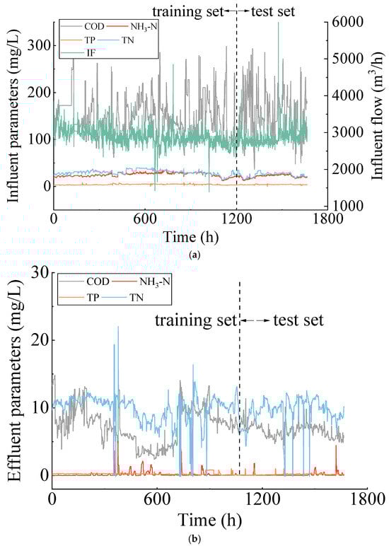
Figure 1.
Time series of water quality measurements: (a) Time series of input influent parameters; (b) time series of output effluent parameters.
2.2. Baseline Models
2.2.1. XGBoost
XGBoost builds upon the Gradient Boosting Decision Tree (GBDT) [41] ensemble learning method by enhancing both its loss function formulation and corresponding optimization process. The main objective of XGBoost is to minimize an objective function that combines two primary terms: the loss term (L) and the regularization term (Ω). Mathematically, the objective function (obj) can be formulated as follows:
During training, XGBoost employs additive learning, where new trees are added to minimize the loss function iteratively. This is different from singular models, which tend to have a pre-defined structure and are optimized in a Euclidean parameter space [42].
2.2.2. Long Short-Term Memory
LSTM [43] is an improved version of the Recurrent Neural Networks (RNNs) created by replacing conventional recurrent nodes with memory cells. As illustrated in Figure 2, each memory cell in LSTM contains three types of gates (i.e., input gate, forget gate, and output gate), implemented as fully connected layers with sigmoid activations to control data flow within the cell. In addition to the gating mechanisms, LSTM networks incorporate an input node, denoted as ct, which serves as the candidate cell state for updating the memory cell. Unlike the gates that typically use the sigmoid activation function, the candidate state employs the hyperbolic tangent (tanh) activation function, mapping values to the range (−1, 1). This design enables the introduction of both positive and negative contributions to the cell’s internal state. The forget gate regulates the extent to which the previous cell state ht−1 is retained; the input gate determines how much of the new candidate information ct is incorporated into the current cell state; and the output gate determines how much of the updated internal state (ct) contributes to the output (ht) at the current timestep. These three gating structures work together to effectively control the selective storage and updating of memory content within the LSTM unit. The internal computational process of LSTM can be described using Equations (2)–(8).
where Wf, Wi, Wc, and Wo are weight matrices; bf, bi, bc, and bo are bias terms; and σ is the sigmoid activation function.
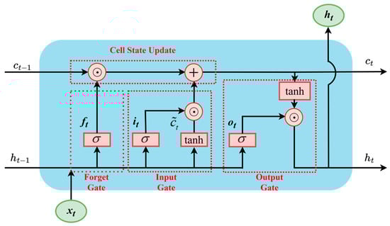
Figure 2.
Internal structure of LSTM unit.
2.3. Interpretable Machine Learning
The XGBoost algorithm offers three importance metrics based on gain, coverage, and weight. In recent years, a model-agnostic method called SHapley Additive exPlanations (SHAP) has become the preferred approach to interpret XGBoost outputs. The following discussion briefly introduces the use of SHAP with XGBoost and the attention mechanism to explain the LSTM model.
2.3.1. SHAP
SHAP was initially proposed by Shapley [44] and computes Shapley values from cooperative game theory; its values explain the contribution of each feature to the prediction. More recently SHAP values have been used as a tool [45] for interpreting ensemble tree models. The specific mathematical expressions of SHAP are shown in Equations (9)–(11) [46]:
where z = {0,1}M, zi = 1 represents a present feature and zi = 0 represents an absent feature; M is the total number of input feature variables; φ0 = f (hx(0)); and φi is the SHAP value:
where F is the set of nonzero inputs in z, S is a subset of the features incorporated into the model, and fx(S) is the prediction for feature values in set S.
2.3.2. Attention Mechanism
The attention mechanism [47] was inspired by the human visual system’s ability to selectively focus on important regions of a scene. Unlike traditional neural network architectures that apply fixed weights to all inputs, the attention mechanism computes a probability distribution over input elements to amplify the impact of the most critical features on the output. To implement the attention mechanism, the raw input data are first transformed into a set of ⟨Key, Value⟩ pairs. The attention module then computes a similarity score between each key and a given Query, which serves as a measure of relevance. These similarity scores are subsequently used to produce a weighted combination of the corresponding values, enabling the model to selectively focus on the most pertinent information in the input sequence. Denoting Query, Key, and Value, respectively, as Q, K, and V, the formulas for calculating weight coefficient W and output a can be expressed as follows:
2.4. Combination of LSTM and XGBoost
LSTM networks excel in capturing both long- and short-term temporal dependencies within time series data. Meanwhile, XGBoost algorithms effectively model nonlinear relationships and mitigate overfitting through regularized optimization. However, neither architecture alone achieves an optimal balance between predictive accuracy and computational efficiency. This underscores the necessity to develop a hybrid framework that synergistically integrates LSTM and XGBoost, thereby establishing an innovative integration methodology to enhance both prediction precision and operational stability in water quality prediction. This paper proposes two approaches combining the LSTM model with an attention mechanism (i.e., Attention–LSTM model) and the XGBoost model. Each integration approach aims to optimize the application of water quality management in wastewater treatment plants. Figure 3 illustrates the two distinct types of integration processes.
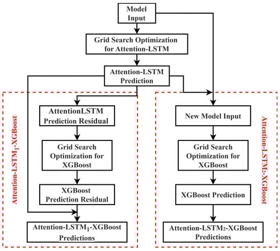
Figure 3.
The LSTM-XGBoost combination process.
The first approach (Attention–LSTM1–XGBoost in the left-hand red-dashed box in Figure 3) leverages the XGBoost model to capture the component of water quality variation not explained by the LSTM model. Specifically, the Attention–LSTM generates the initial predicted values yAttention-LSTM and the residual εAttention-LSTM between the predicted values and the actual values is computed. Then the XGBoost model is trained on these residuals to obtain the predicted residuals εXGBoost. The final prediction is obtained by summing yAttention-LSTM and εXGBoost. This hybrid configuration is referred to as the Attention–LSTM1–XGBoost model.
The second approach (Attention–LSTM2–XGBoost in the right-hand red-dashed box in Figure 3) utilizes the temporal features extracted by Attention–LSTM to assist the XBoost model in water quality prediction. First, the Attention–LSTM model is trained on time series data to obtain predicted value yAttention-LSTM. The obtained prediction is concatenated with the original independent variables to form a new input. The XGBoost model is trained on this combined input to generate the final predicted value. This hybrid model is referred to as the Attention–LSTM2–XGBoost model.
2.5. Hyperparameter Optimization
Grid search performs exhaustive optimization by discretizing all possible parameter combinations into a grid within the parameter space and evaluating each combination. For each parameter combination, cross-validation is used to calculate the error, and the combination with the minimum error is selected as the global optimal solution. Grid search is effective in finding the optimal solution from multiple parameters. Therefore, in this study, we employ grid search to determine the optimal hyperparameters for both the XGBoost and LSTM models. For the XGBoost model, the search space included n_estimators, which determines the number of weak learners; max_depth, which limits tree depth to prevent overfitting; learning_rate, which adjusts the contribution of each tree; subsample, which controls the proportion of data sampled for training each tree; and child_weight, which controls the weight of splits at child nodes. For the LSTM model, grid search optimizes epochs representing the number of full training passes; batch size defines the number of samples used in each training step; units control the number of LSTM units and thus the model’s expressive capacity; and timestep refers to the number of timesteps in each input sequence and thus influences the model’s temporal context.
Figure 4 illustrates the example of a grid search procedure applied to the model’s parameters. The selection ranges of all hyperparameters are listed in Table 1. Hyperparameter selection ranges for different models were determined based on the characteristics of the time series dataset collected in this work.
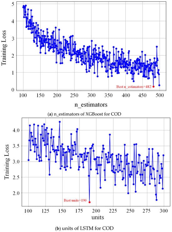
Figure 4.
Conducting a grid search for XGBoost and LSTM parameters: (a) n_estimators of XGBoost for COD; (b) units of LSTM for COD.

Table 1.
Hyperparameters for different prediction models.
3. Results and Discussion
3.1. Statistical Analysis
Before training the model, a statistical analysis of the dataset was performed, calculating the correlation between all measurements at the wastewater treatment plant, including both input and output variables. Figure 5 presents the heat map of correlation coefficients in the dataset. As can be observed, there is a notable correlation between NH3-H and TN among the input variables, and COD and IF demonstrate statistically weak correlations with all other parameters in the feature space. In contrast, the correlation among the output variables is relatively weak.
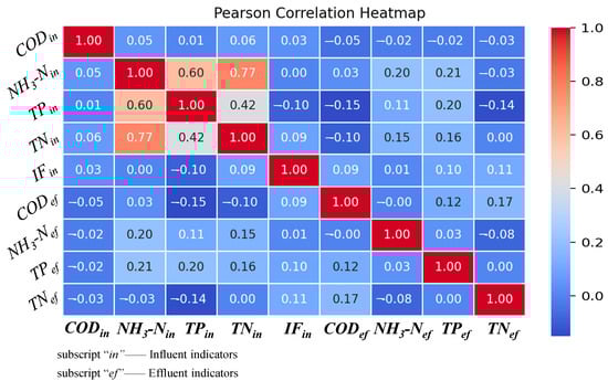
Figure 5.
Heat map of correlation between input and output variables in dataset.
3.2. Performance of Singular Models
Figure 6 and Figure 7 show the predicted effluent parameters obtained from the trained LSTM and XGBoost models compared to the measured data. The black line indicates the actual measurements, while the red line shows the predicted values. The prediction performance evaluation metrics of the three singular machine learning methods are listed in Table 2. The results indicate that the LSTM model demonstrates a marginally better performance compared to the XGBoost model on the training set. Specifically, the R2 values for LSTM are 0.896 and 0.873 for COD and NH3-N, respectively, while the R2 values for XGBoost are 0.893 and 0.855 for COD and NH3-N, respectively. Additionally, for the three effluent parameters—COD, NH3-N, and TP—the model fitting results on the training set are consistently below the measured values. On the test set, the predictive performance of the LSTM and XGBoost models is largely comparable. The R2 for the two models across different effluent parameters are all above 0.800. However, it is important to note that the prediction performance should not be solely evaluated based on the value of R2. For instance, while the LSTM model yields a R2 for the COD parameter compared to the XGBoost model, its RMSE and MAE values are also higher. Furthermore, the Attention–LSTM model, which incorporates the attention mechanism, outperforms the previous two models both on the training and test sets, demonstrating its superior generalization capability (Figure 8). In short, the LSTM, XGBoost, and Attention–LSTM models are capable of effectively approximating the irregular periodicity of effluent parameters during the measurement period.
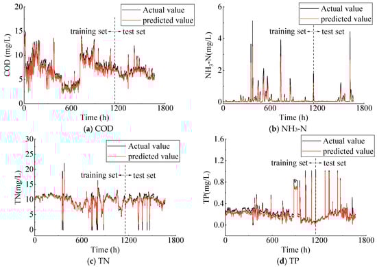
Figure 6.
Actual vs. predicted values of effluent parameters using LSTM model.
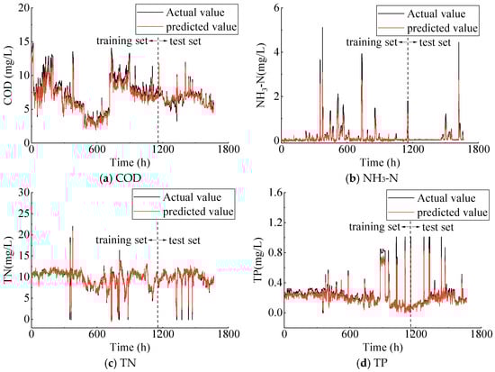
Figure 7.
Actual vs. predicted values of effluent parameters using XGBoost model.
Table 2.
Performance indicators of effluent COD, NH3-N, TN, and TP using singular models.
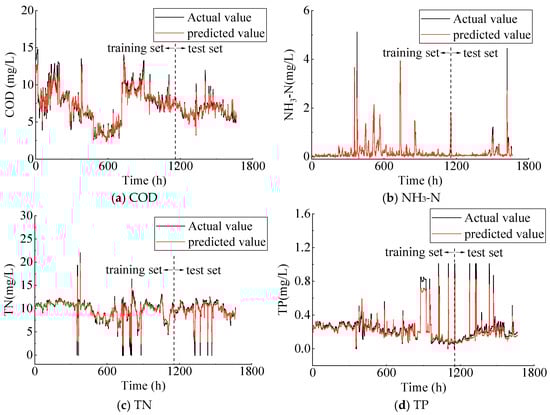
Figure 8.
Actual vs. predicted values of effluent parameters using Attention–LSTM model.
3.3. Interpretability Analysis
For the four effluent parameters, Figure 9 presents the feature importance ranking of the five input variables, derived using three interpretability analysis methods. The vertical axis represents the normalized score. These methods include the weight method of XGBoost, the SHAP method, and the attention mechanism method. Overall, the SHAP and attention mechanism methods exhibit a high degree of consistency in the feature importance ranking. Specifically, for effluent TN prediction, both methods rank influent TN, TP, and NH3-N in the top three, which may be attributed to NH3-N being an essential component of TN. For effluent NH3-N prediction, both methods prioritize influent NH3-N as the most important feature, while ranking influent flow rate as the least significant. These results align with conclusions drawn in existing research [48,49]. In contrast, the feature importance ranking generated by the weight method of XGBoost demonstrates greater variability across the four effluent parameters. For example, influent COD, NH3-N, and IF are ranked among the top three for effluent TN prediction, and influent COD is ranked first for effluent NH3-N prediction. This may be due to the fact that when there is multicollinearity among features, XGBoost tends to prioritize splitting one feature, potentially overlooking other correlated features. It is also worth noting that even the lower-ranked features in Figure 9 may demonstrate scores that are not substantially lower than those of higher-ranked features. For example, NH3-N shows a certain degree of contribution to the predicted COD time series, as indicated by SHAP values. This may be attributed to the indirect relationships between the volume of food scraps, excreta, and washing wastewater generated by residents [50]. Additionally, NH3-N in water can undergo transformation through microbial processes under specific conditions. Under aerobic conditions, nitrification consumes oxygen, which may result in a decrease in available oxygen, thereby potentially affecting the oxidation of organic matter.
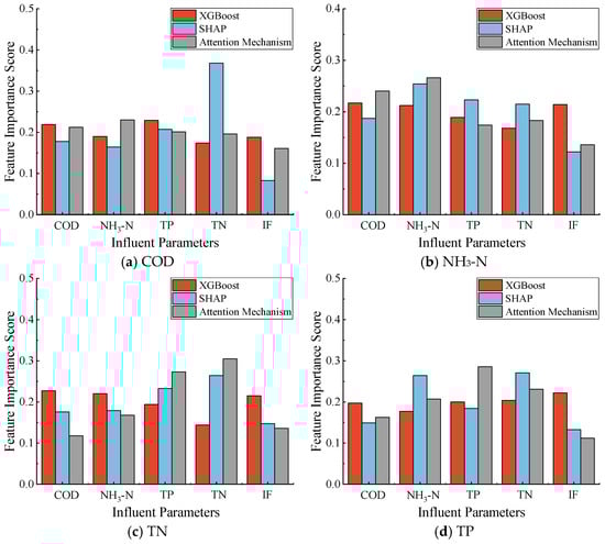
Figure 9.
Feature importance ranking for effluent: (a) COD; (b) NH3-N; (c) TP; (d) TP.
Figure 10 illustrates the significant interactions between input parameters in the prediction of COD using XGBoost. On the right side of each plot, a color bar is provided to represent the interacting input parameters, with blue and red corresponding to lower and higher values, respectively. Taking Figure 10a as an example, the partial dependence relationship between the influent TP and TN is depicted. The figure demonstrates that the effect of influent TN on effluent COD is dependent on the TN range. Notably, when the influent TP concentration is high, the negative correlation between influent TN and effluent COD becomes more pronounced. This observed trend highlights the intricate interaction between influent TN and influent TP.
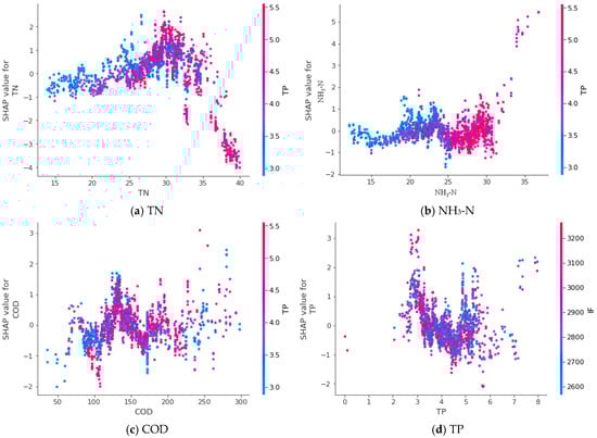
Figure 10.
SHAP dependence scatter plots with interactions for predicting COD.
3.4. Performance of Hybrid Models
Figure 11 and Figure 12 present the results from the two hybrid models, while Table 3 provides the specific values of the performance metrics. It is evident that, regardless of the training or test set used, the Attention–LSTM1–XGBoost and Attention–LSTM2–XGBoost models outperform the previous three models across all four effluent parameters. A notable observation is that neither of the two hybrid models exhibits a consistent underestimation of certain parameters throughout the entire monitoring period, as was observed in the previous case with a singular model (e.g., as seen in Figure 6). Throughout the entire period, both models displayed relatively large errors during the TP prediction phase (around the 900th hour), as seen in Figure 11d and Figure 12d. However, the error values remained substantially lower compared to those of the singular model. Furthermore, neither of the two hybrid models exhibited the prediction delay typically observed in traditional autoregressive models. The two hybrid models exhibit an outstanding performance in forecasting effluent quality values. In the case of the training dataset, the minimum R2 value of 0.953 and the maximum R2 value of 0.995 signify a good alignment with the actual values. For the test set, a more detailed quantitative analysis reveals that the Attention–LSTM1–XGBoost model achieves R2 values of 0.972, 0.957, and 0.952 for predicting COD, TN, and TP, respectively. It demonstrates increases in R2 of 2.1%, 1.2%, and 4.2% for these three metrics compared to the Attention–LSTM2–XGBoost model. However, the Attention-LSTM2-XGBoost model demonstrates slightly superior predictive performance for NH3-N compared to the Attention–LSTM1–XGBoost model, with an increase in R2 of 0.4%, along with reductions in RMSE and MAE of 8.8% and 25.0%, respectively. In summary, LSTM networks are particularly adept at capturing both long-term and short-term temporal dependencies in time series data. In contrast, XGBoost algorithms are highly effective at modeling nonlinear relationships and reducing overfitting through regularization-based optimization techniques. Attention–LSTM1–XGBoost utilizes the information by adjusting the residuals, while Attention–LSTM2–XGBoost enhances the input features through the extraction of temporal dependencies. These two hybrid models leverage the respective strengths of the XGBoost and LSTM models from distinct perspectives, resulting in a substantial improvement in both predictive performance and generalization capability.
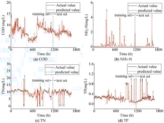
Figure 11.
Actual vs. predicted values of effluent parameters using Attention–LSTM1–XGBoost model.
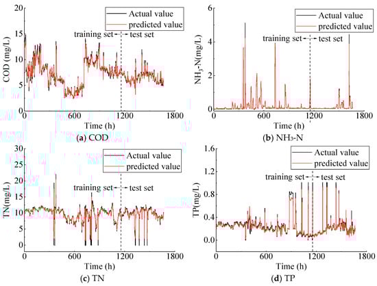
Figure 12.
Actual vs. predicted values of effluent parameters using Attention–LSTM2–XGBoost model.
Table 3.
Performance indicators of effluent COD, NH3-N, TN, and TP using hybrid models.
4. Conclusions
This paper presents two hybrid models that integrate LSTM and XGBoost to predict four effluent parameters in wastewater treatment plants, and compares their performance against three singular machine learning models. The key findings are summarized as follows:
- (1)
- The predictive performance of the individual LSTM and XGBoost models is relatively comparable, with R2 values for the four effluent parameters ranging from 0.810 to 0.877. However, the predictions for certain parameters exhibit a consistent underestimation of the actual values throughout the monitoring period. In contrast, the LSTM model incorporating the attention mechanism demonstrates improved predictive accuracy, with R2 values ranging from 0.850 to 0.899.
- (2)
- Interpretability analysis reveals that the feature importance rankings from SHAP and the attention mechanism are largely consistent. For a given effluent parameter, in addition to the corresponding influent parameter, other influent indicators also influence the outcome through interactions. However, the rankings from the weight method of XGBoost differ from those of SHAP and the attention mechanism. This discrepancy may result from XGBoost’s tendency to prioritize a single feature for splitting, disregarding other correlated features.
- (3)
- The prediction accuracy of the two hybrid models is markedly superior to that of the singular model. The first model utilizes the information by adjusting the residuals, achieving R2 values ranging from 0.952 to 0.982. The second model enhances the input features by capturing temporal dependencies, resulting in R2 values between 0.914 and 0.986. The hybrid framework strategically combines the strengths of XGBoost and LSTM models from complementary perspectives, offering a robust solution for treatment process stability evaluation and real-time effluent quality monitoring. This integration has the potential to enable proactive adjustments in wastewater treatment processes, thereby optimizing operational efficiency and improving system responsiveness and treatment system resilience.
The hydraulic retention time of the sewage biochemical treatment process is usually several hours or may even be more than ten hours. For operational parameter adjustment, using predictions based on the influent quality and flow rate as the feedforward parameters, and hence predicting the future effluent quality, has better sensitivity than methods using the biochemical process parameters or effluent quality feedback. Therefore, based on the effluent quality in the next few hours, operators of wastewater treatment plants can adjust the operational parameters on their initiative to ensure effluent quality is stable and up to regulated discharge standards.
The hybrid model framework has great potential to evaluate process stability in wastewater treatment plants, paving the way for smarter, more resilient, and more sustainable wastewater management with predictive control and real-time process monitoring, which will improve ecological integrity and regulatory compliance. WWTPs are transformed from reactive to predictive sentinels of public health and environmental integrity. By ensuring effluent meets stringent quality standards, the methods mitigate downstream pollution, protect ecosystems, conserve resources, and reduce human exposure to contaminants. As climate change intensifies water stress and regulatory pressures, smart effluent management will become indispensable for sustainable water cycles.
In the future, according to the different working conditions of a wastewater treatment plant, the mechanistic model and data-driven model can be combined to evaluate the response-ability of the biochemical reaction process facing impact loads, and can meanwhile achieve the adjustment and optimization of operating parameters. Future advancements in edge computing and digital twins will also further amplify these benefits, embedding wastewater treatment into the One Health framework.
Author Contributions
Conceptualization, Z.X. and Z.L.; methodology, X.L.; validation, Z.X. and X.L.; formal analysis, Z.L.; resources, Z.X.; data curation, Z.X.; writing—original draft preparation, Z.X. and X.L.; writing—review and editing, T.I.; visualization, T.I.; supervision, Y.C.; project administration, Y.C. All authors have read and agreed to the published version of the manuscript.
Funding
This research received no external funding.
Data Availability Statement
The data presented in this study are available on request from the corresponding author due to data security requirements.
Conflicts of Interest
The authors declare no conflicts of interest.
References
- Silva, J.A. Wastewater treatment and reuse for sustainable water resources management: A systematic literature review. Sustainability 2023, 15, 10940. [Google Scholar] [CrossRef]
- Wang, M.; Bodirsky, B.L.; Rijneveld, R.; Beier, F.; Bak, M.P.; Batool, M.; Droppers, B.; Popp, A.; van Vliet, M.T.H.; Strokal, M. A triple increase in global river basins with water scarcity due to future pollution. Nat. Commun. 2024, 15, 880. [Google Scholar] [CrossRef] [PubMed]
- Newhart, K.B.; Holloway, R.W.; Hering, A.S.; Cath, T.Y. Data-driven performance analyses of wastewater treatment plants: A review. Water Res. 2019, 157, 498–513. [Google Scholar] [CrossRef] [PubMed]
- Flores-Alsina, X.; Ramin, E.; Ikumi, D.; Harding, T.; Batstone, D.; Brouckaert, C.; Sotemann, S.; Gernaey, K.V. Assessment of sludge management strategies in wastewater treatment systems using a plant-wide approach. Water Res. 2021, 190, 116714. [Google Scholar] [CrossRef]
- Feng, K.; Zhao, Z.; Li, M.; Tian, L.; An, T.; Zhang, J.; Xu, X.; Zhu, L. Novel intelligent control framework for WWTP optimization to achieve stable and sustainable operation. ACS ES&T Eng. 2022, 2, 2086–2094. [Google Scholar] [CrossRef]
- Jin, T.; Cai, S.; Jiang, D.; Liu, J. A data-driven model for real-time water quality prediction and early warning by an integration method. Environ. Sci. Pollut. Res. 2019, 26, 30374–30385. [Google Scholar] [CrossRef] [PubMed]
- Gujer, W.; Henze, M.; Mino, T.; Matsuo, T.; Wentzel, M.C.; Marais, G.V.R. The activated sludge model No. 2: Biological phosphorus removal. Water Sci. Technol. 1995, 31, 1–11. [Google Scholar] [CrossRef]
- Gujer, W.; Henze, M.; Mino, T.; Van Loosdrecht, M. Activated sludge model No. 3. Water Sci. Technol. 1999, 39, 183–193. [Google Scholar] [CrossRef]
- Henze, M.; Gujer, W.; Mino, T.; Matsuo, T.; Wentzel, M.C.; Marais, G.V.R.; Van Loosdrecht, M.C. Activated sludge model no. 2d, ASM2d. Water Sci. Technol. 1999, 39, 165–182. [Google Scholar] [CrossRef]
- Zhu, J.-J.; Kang, L.; Anderson, P.R. Predicting influent biochemical oxygen demand: Balancing energy demand and risk management. Water Res. 2018, 128, 304–313. [Google Scholar] [CrossRef]
- Bolyard, S.C.; Reinhart, D.R. Evaluation of leachate dissolved organic nitrogen discharge effect on wastewater effluent quality. Waste Manag. 2017, 65, 47–53. [Google Scholar] [CrossRef] [PubMed]
- El Shorbagy, W.E.; Radif, N.N.; Droste, R.L. Optimization of A2O BNR Processes Using ASM and EAWAG Bio-P Models: Model Performance. Water Environ. Res. 2013, 85, 2271–2284. [Google Scholar] [CrossRef]
- Jeppsson, U.; Alex, J.; Batstone, D.J.; Benedetti, L.; Comas, J.; Copp, J.B.; Corominas, L.; Flores-Alsina, X.; Gernaey, K.V.; Nopens, I.; et al. Benchmark simulation models, quo vadis? Water Sci. Technol. 2013, 68, 1–15. [Google Scholar] [CrossRef] [PubMed]
- Wan, W.; Yang, L.; Liu, L.; Zhang, Z.; Jia, R.; Choi, Y.-K.; Pan, J.; Theobalt, C.; Komura, T.; Wang, W. Learn to predict how humans manipulate large-sized objects from interactive motions. IEEE Robot. Autom. Lett. 2022, 7, 4702–4709. [Google Scholar] [CrossRef]
- Lin, S.; Kim, J.; Hua, C.; Park, M.-H.; Kang, S. Coagulant dosage determination using deep learning-based graph attention multivariate time series forecasting model. Water Res. 2023, 232, 119665. [Google Scholar] [CrossRef] [PubMed]
- Xie, C.; Yang, X.; Chen, T.; Fang, Q.; Wang, J.; Shen, Y. Short-term wind power prediction framework using numerical weather predictions and residual convolutional long short-term memory attention network. Eng. Appl. Artif. Intell. 2024, 133, 108543. [Google Scholar] [CrossRef]
- Zhang, S.; Yu, W.; Zhang, W. Interactive dynamic diffusion graph convolutional network for traffic flow prediction. Inf. Sci. 2024, 677, 120938. [Google Scholar] [CrossRef]
- Li, S.; Zhang, R. A novel interactive deep cascade spectral graph convolutional network with multi-relational graphs for disease prediction. Neural Netw. 2024, 175, 106285. [Google Scholar] [CrossRef]
- Liao, S.; Xie, L.; Du, Y.; Chen, S.; Wan, H.; Xu, H. Stock trend prediction based on dynamic hypergraph spatio-temporal network. Appl. Soft Comput. 2024, 154, 111329. [Google Scholar] [CrossRef]
- Zhao, Y.; Guo, L.; Liang, J.; Zhang, M. Seasonal artificial neural network model for water quality prediction via a clustering analysis method in a wastewater treatment plant of China. Desalin. Water Treat. 2016, 57, 3452–3465. [Google Scholar] [CrossRef]
- Jawad, J.; Hawari, A.H.; Zaidi, S.J. Artificial neural network modeling of wastewater treatment and desalination using membrane processes: A review. Chem. Eng. J. 2021, 419, 129540. [Google Scholar] [CrossRef]
- Zhang, L.; Chao, B.; Zhang, X. Modeling and optimization of microbial lipid fermentation from cellulosic ethanol wastewater by Rhodotorula glutinis based on the support vector machine. Bioresour. Technol. 2020, 301, 122781. [Google Scholar] [CrossRef] [PubMed]
- Hejabi, N.; Saghebian, S.M.; Aalami, M.T.; Nourani, V. Evaluation of the effluent quality parameters of wastewater treatment plant based on uncertainty analysis and post-processing approaches (case study). Water Sci. Technol. 2021, 83, 1633–1648. [Google Scholar] [CrossRef]
- Pham, Q.B.; Gaya, M.; Abba, S.; Abdulkadir, R.; Esmaili, P.; Linh, N.T.T.; Sharma, C.; Malik, A.; Khoi, D.N.; Dung, T.D.; et al. Modeling of Bunus regional sewage treatment plant using machine learning approaches. Desalin. Water Treat. 2020, 203, 80–90. [Google Scholar] [CrossRef]
- Mekaoussi, H.; Heddam, S.; Bouslimanni, N.; Kim, S.; Zounemat-Kermani, M. Predicting biochemical oxygen demand in wastewater treatment plant using advance extreme learning machine optimized by Bat algorithm. Heliyon 2023, 9, e21351. [Google Scholar] [CrossRef]
- Cheng, Q.; Chunhong, Z.; Qianglin, L. Development and application of random forest regression soft sensor model for treating domestic wastewater in a sequencing batch reactor. Sci. Rep. 2023, 13, 9149. [Google Scholar] [CrossRef]
- Zhou, P.; Li, Z.; Snowling, S.; Baetz, B.W.; Na, D.; Boyd, G. A random forest model for inflow prediction at wastewater treatment plants. Stoch. Environ. Res. Risk Assess. 2019, 33, 1781–1792. [Google Scholar] [CrossRef]
- Gao, J.; Wahlen, A.; Ju, C.; Chen, Y.; Lan, G.; Tong, Z. Reinforcement learning-based control for waste biorefining processes under uncertainty. Commun. Eng. 2024, 3, 38. [Google Scholar] [CrossRef]
- Negm, A.; Ma, X.; Aggidis, G. Deep reinforcement learning challenges and opportunities for urban water systems. Water Res. 2024, 253, 121145. [Google Scholar] [CrossRef]
- Yang, Q.; Cao, W.; Meng, W.; Si, J. Reinforcement-learning-based tracking control of waste water treatment process under realistic system conditions and control performance requirements. IEEE Trans. Syst. Man Cybern. Syst. 2021, 52, 5284–5294. [Google Scholar] [CrossRef]
- Xu, B.; Pooi, C.K.; Tan, K.M.; Huang, S.; Shi, X.; Ng, H.Y. A novel long short-term memory artificial neural network (LSTM)-based soft-sensor to monitor and forecast wastewater treatment performance. J. Water Process Eng. 2023, 54, 104041. [Google Scholar] [CrossRef]
- Voipan, D.; Voipan, A.E.; Barbu, M. Evaluating Machine Learning-Based Soft Sensors for Effluent Quality Prediction in Wastewater Treatment Under Variable Weather Conditions. Sensors 2025, 25, 1692. [Google Scholar] [CrossRef]
- Yin, H.; Chen, Y.; Zhou, J.; Xie, Y.; Wei, Q.; Xu, Z. A probabilistic deep learning approach to enhance the prediction of wastewater treatment plant effluent quality under shocking load events. Water Res. X 2025, 26, 100291. [Google Scholar] [CrossRef] [PubMed]
- Zhu, B. COD Prediction Model for Wastewater Treatment Based on Particle Swarm Algorithm. In Proceedings of the 2023 Asia-Europe Conference on Electronics, Data Processing and Informatics (ACEDPI), Prague, Czech Republic, 7–19 April 2023; pp. 454–459. [Google Scholar]
- Xie, Y.; Chen, Y.; Wei, Q.; Yin, H. A hybrid deep learning approach to improve real-time effluent quality prediction in wastewater treatment plant. Water Res. 2024, 250, 121092. [Google Scholar] [CrossRef]
- Yao, Z.; Wang, Z.; Huang, J.; Xu, N.; Cui, X.; Wu, T. Interpretable prediction, classification and regulation of water quality: A case study of Poyang Lake, China. Sci. Total Environ. 2024, 951, 175407. [Google Scholar] [CrossRef]
- Zhang, Y.; Li, C.; Jiang, Y.; Sun, L.; Zhao, R.; Yan, K.; Wang, W. Accurate prediction of water quality in urban drainage network with integrated EMD-LSTM model. J. Clean. Prod. 2022, 354, 131724. [Google Scholar] [CrossRef]
- Chen, Y.; Zhang, H.; You, Y.; Zhang, J.; Tang, L. A hybrid deep learning model based on signal decomposition and dynamic feature selection for forecasting the influent parameters of wastewater treatment plants. Environ. Res. 2025, 266, 120615. [Google Scholar] [CrossRef]
- Lv, J.-Q.; Yin, W.-X.; Xu, J.-M.; Cheng, H.-Y.; Li, Z.-L.; Yang, J.-X.; Wang, A.-J.; Wang, H.-C. Augmented machine learning for sewage quality assessment with limited data. Environ. Sci. Ecotechnol. 2025, 23, 100512. [Google Scholar] [CrossRef]
- Chen, T.; Guestrin, C. Xgboost: A scalable tree boosting system. In Proceedings of the 22nd ACM SIGKDD International Conference on Knowledge Discovery and Data Mining, San Francisco, CA, USA, 13–17 August 2016; pp. 785–794. [Google Scholar]
- Friedman, J.H. Greedy function approximation: A gradient boosting machine. Ann. Stat. 2001, 29, 1189–1232. [Google Scholar] [CrossRef]
- Ching, P.; Zou, X.; Wu, D.; So, R.; Chen, G. Development of a wide-range soft sensor for predicting wastewater BOD5 using an eXtreme gradient boosting (XGBoost) machine. Environ. Res. 2022, 210, 112953. [Google Scholar] [CrossRef]
- Hochreiter, S.; Schmidhuber, J. Long short-term memory. Neural Comput. 1997, 9, 1735–1780. [Google Scholar] [CrossRef] [PubMed]
- Shapley, L.S. 17. A Value for n-Person Games. In Contributions to the Theory of Games; Kuhn, H.W., Tucker, A.W., Eds.; Princeton University Press: Princeton, NJ, USA, 2016; Volume II, pp. 307–318. Available online: https://www.degruyterbrill.com/document/doi/10.1515/9781400881970-018/html (accessed on 19 June 2025).
- Lundberg, S.M.; Lee, S.I. A unified approach to interpreting model predictions. In Proceedings of the 31st International Conference on Neural Information Processing Systems, Long Beach, CA, USA, 4–9 December 2017. [Google Scholar]
- Deng, Z.; Wan, J.; Ye, G.; Wang, Y. Data-driven prediction of effluent quality in wastewater treatment processes: Model performance optimization and missing-data handling. J. Water Process Eng. 2025, 71, 107352. [Google Scholar] [CrossRef]
- Treisman, A.M.; Gelade, G. A feature-integration theory of attention. Cogn. Psychol. 1980, 12, 97–136. [Google Scholar] [CrossRef] [PubMed]
- Zhu, J.; Wagner, M.; Cornel, P.; Chen, H.; Dai, X. Feasibility of on-site grey-water reuse for toilet flushing in China. J. Water Reuse Desalin. 2018, 8, 1–13. [Google Scholar] [CrossRef]
- Simbeye, C.; Courtney, C.; Simha, P.; Fischer, N.; Randall, D.G. Human urine: A novel source of phosphorus for vivianite production. Sci. Total Environ. 2023, 892, 164517. [Google Scholar] [CrossRef]
- Zhang, Y.; Wang, J.; Li, C.; Duan, H.; Wang, W. Attention-based deep learning models for predicting anomalous shock of wastewater treatment plants. Water Res. 2025, 275, 123192. [Google Scholar] [CrossRef]
Disclaimer/Publisher’s Note: The statements, opinions and data contained in all publications are solely those of the individual author(s) and contributor(s) and not of MDPI and/or the editor(s). MDPI and/or the editor(s) disclaim responsibility for any injury to people or property resulting from any ideas, methods, instructions or products referred to in the content. |
© 2025 by the authors. Licensee MDPI, Basel, Switzerland. This article is an open access article distributed under the terms and conditions of the Creative Commons Attribution (CC BY) license (https://creativecommons.org/licenses/by/4.0/).