Similar Physical Model Experimental Investigation of Landslide-Induced Impulse Waves Under Varying Water Depths in Mountain Reservoirs

Abstract

Landslide-induced impulse waves (LIIWs) are significant natural hazards, frequently occurring in mountain reservoirs, which threaten the safety of waterways and dam project. To predict the impact of impulse waves induced by Rongsong (RS) potential landslide on the dam, during the layered construction period and maximum water level operation period of Rumei (RM) Dam (unbuilt), a large-scale three-dimensional similar physical model with a similarity scale of 200:1 (prototype length to model length) was established. The experiments set five water levels during the dam’s layered construction period and recorded and analyzed the generation and propagation laws of LIIWs. The findings indicate that, for partially granular submerged landslides, no splashing waves are generated, and the waveform of the first wave remains intact. The amplitude of the first wave exhibits stable attenuation while the third one reaches the largest. After the first three columns of impulse waves, water on the dam surface oscillates between the two banks. This study specifically discusses the impact of different water depths on LIIWs. The results show that the wave height increases as the water depth decreases. Two empirical formulas to calculate the wave attenuation at the generation area and to calculate the maximum vertical run-up height on the dam surface were derived, showing strong agreement between the empirical formulas and experimental values. Based on the model experiment results, the wave height data in front of the RM dam during the construction and operation periods of the RM reservoir were predicted, and engineering suggestions were given for the safety height of the cofferdam during the construction and security measures to prevent LIIW overflow the dam top during the operation periods of the RM dam.

1. Introduction

Landslide-induced impulse waves (LIIWs) are considered significant secondary hazards, sometimes more destructive than the landslide itself, especially in the reservoir areas [1]. The Vajont disaster, which occurred on 9 October 1963, is one of the most catastrophic documented instances of LIIWs [2]. A 300 million m³ landslide near the dam detached and fell into the Vajont reservoir, generating an 80 m high wave. The impulse wave overtopped the Vajont dam and destroyed the city of Longarone, resulting in the death of 1909 people [3]. Evaluating LIIWs in reservoirs is crucial for the planning and management of dams and the reservoirs [2]. Research on LIIW characteristics in reservoir areas is essential for hazard prediction and mitigation.

Current methods used to investigate the generation and the propagation of LIIWs can be divided into numerical simulations and model experiments. Recent research has seen numerical simulations evolve from a single method to multiple approaches, including DEM-SPH [4,5], CFD-DEM [6], and SPH-SWEs [7]. Numerical simulation [8,9,10,11] plays a key role in calculating LIIWs under known parameter conditions. However, due to the complex terrain of mountain reservoir river channels and the complex coupling mechanism between water flow and landslides, many parameters remain difficult to obtain accurately, making it challenging to ensure the accuracy of numerical simulation results.

The physical model experiment method is widely used as an effective method for studying LIIWs. Initially, researchers investigated the characteristics of LIIWs through simplified two-dimensional model experiments with different materials like 2D block materials [12,13,14,15,16,17,18,19,20] and 2D granular materials [21,22,23,24,25,26,27,28,29,30,31,32,33]. Additionally, some researchers conducted two-dimensional experiments with various landslide materials under different water conditions. For example, Tang [34] used a combination of block and granular materials, while Meng [35] employed a visco-plastic material. Also, pure water [36] and debris flow [37] were chosen as water environments., Through these two-dimensional model experiments, researchers examined the characteristics of LIIWs along the sliding axis, such as waveform classification, wave amplitude/height trends, wave period, wavelength, wave speed, and wave run-up along the opposite-bank slope.

Due to the constraint effects of the narrow side walls of two-dimensional experiments, researchers began conducting experiments in unconfined water using three-dimensional model setups, which more closely replicate real phenomena. Prior to the use of large-sized 3D water basins, medium-sized water basins (2.5D) were also used as an intermediate step between 2D and 3D. The characteristics of medium-sized water basins were that their width was less than 2.5 m, but still much larger than the width of the landslide [38,39,40,41,42]. In 3D experiments, block materials [43,44,45,46,47,48,49,50] and granular materials [51,52,53,54,55,56] were used. Through three-dimensional model experiments, researchers investigated the characteristics of LIIWs both along the sliding axis and across axes with different deflection angles on the water surface.

The two-dimensional and three-dimensional LIIW model experiments discussed above were conducted in regular terrain, which should be called theoretical model experiments. Due to the complexity of real engineering terrain and landslide movement, the laws of theoretical model experiments are difficult to apply to real engineering. Especially for reservoir landslides, the direction of wave propagation is perpendicular to the direction of landslide movement, while in theoretical model experiments, the direction of wave propagation follows the direction of landslide movement. This has led to a completely different propagation pattern of landslide surges in the reservoir from the theoretical model experiments.

To study the characteristics of LIIWs in practical engineering projects, researchers established three-dimensional scaled physical models with proportionally reduced terrains. Huang [57] used marble coarse sand material and set four test water depths, recording wave height data along sliding axis and at the center of the river channel. Wang [58,59] used cement gravel blocks and varied block shapes, water depths, opposite-bank slope feet, inflow angles, and inflow velocities, proposing empirical formulas for maximum wave height and opposite-bank climb height. Chen [60] used pebbles and varied sliding speeds, recording wave height data along sliding axis and at the center of the river channel, and proposed an empirical formula for dam surface climbing.

Compared to 2D and 3D experiments conducted in regular terrain, the results of similarity physical model experiments are more representative of real engineering scenarios [57]. However, due to the high construction cost and monitoring equipment costs associated with large-scale model experiments, there are still relatively few large-scale similar model experiments at present. The complex geometric shapes of landslide bodies, intricate river terrain, and other factors make the patterns observed during wave height propagation more complex. This makes the results and patterns of similar physical model experiments only applicable to projects with similar terrain.

Therefore, in order to predict the LIIWs in a specific project, a three-dimensional similar physical model should be established based on the terrain of the project. In order to predict the impact of impulse waves induced by Rongsong (RS) potential landslide on the dam during the layered construction period and maximum water level operation period of Rumei (RM) Dam (unbuilt), this paper establishes a large-scale 3D similar physical model based on the terrain of RM reservoir, sets five construction period water levels, and records and analyzes the generation and propagation laws of LIIWs in RM reservoir at different water depths. The wave height data in front of the dam surface recorded in the experiment is used to guide the safety during the RM dam construction period and reservoir operation period. The results of model experiments help researchers understand the generation and propagation laws of LIIWs in mountain reservoir terrain, expand the database of LIIW experiments in complex terrain, provide data support for fluid–solid coupling research, and fluid motion research in complex terrain.

2. Methodology

2.1. Similarity Theory

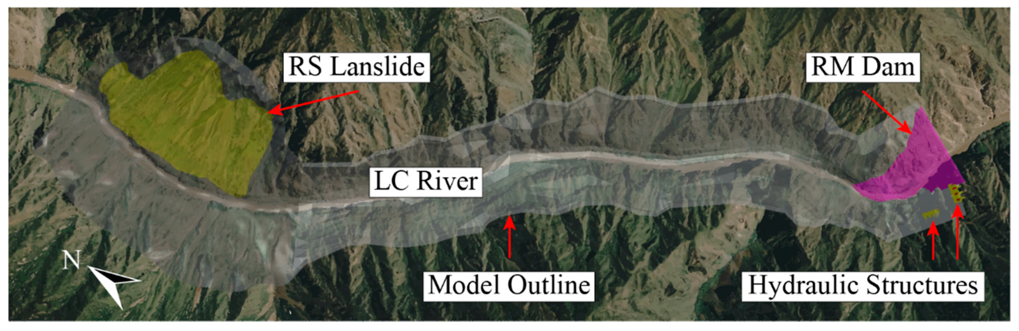
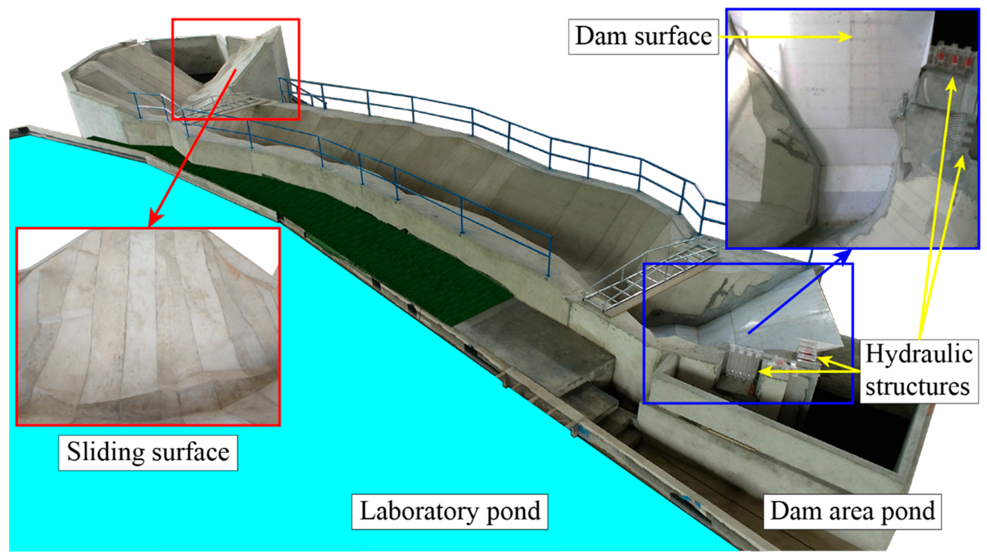
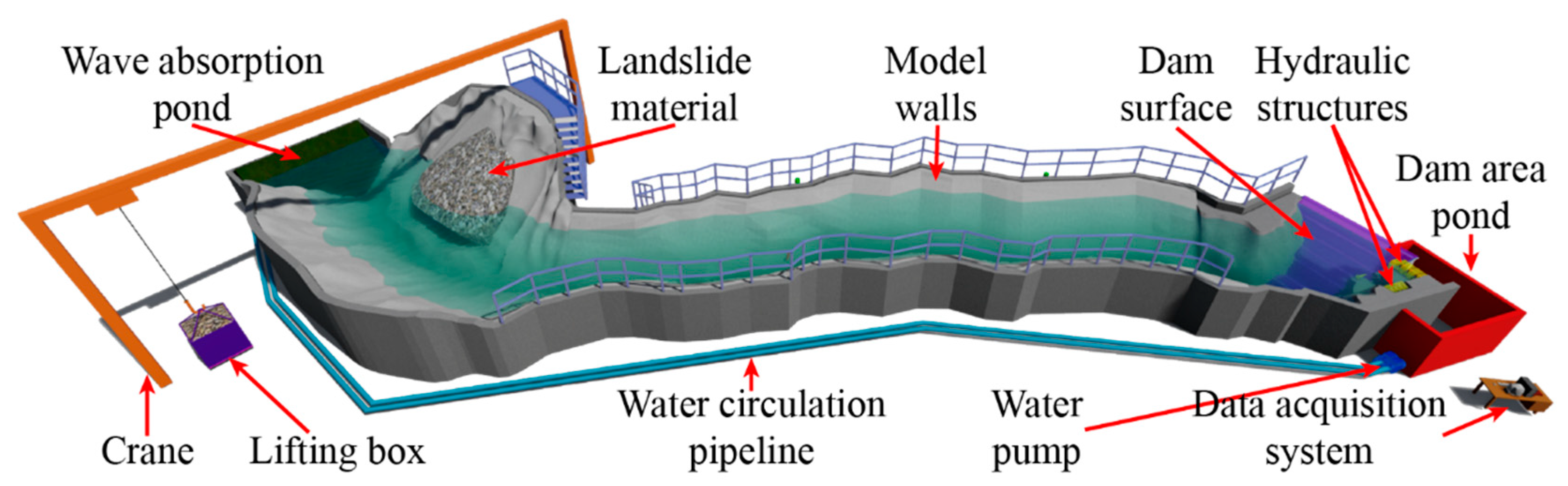
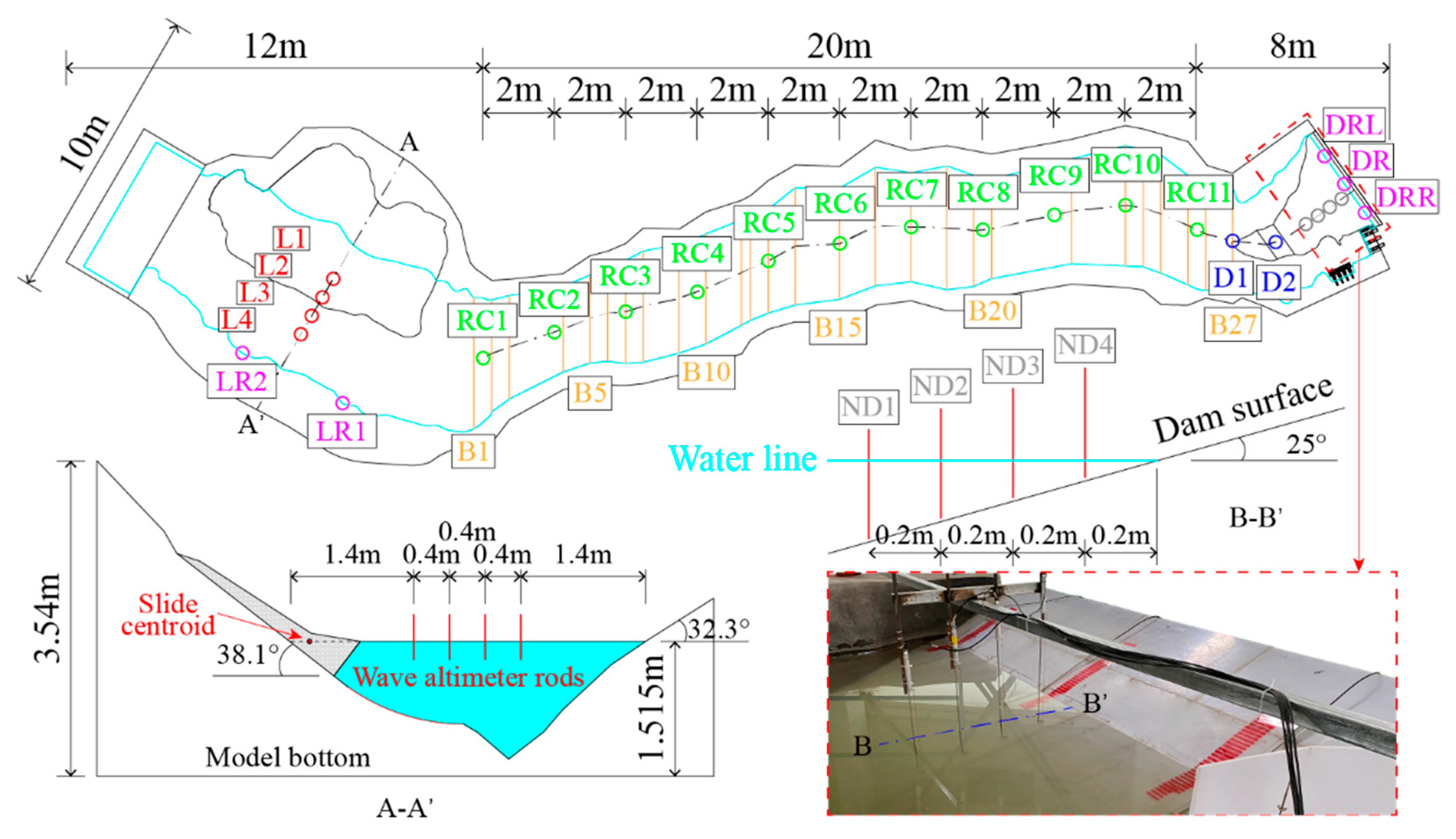
The model is established based on similarity theory, satisfying geometric similarity, water flow motion similarity, dynamic similarity, and following Froude similarity criterion. According to Newton’s similarity criterion, when gravity is the main force, gravity scale and inertial force scale should be equal.

Defining $L_r=L_p/L_m$, where $L$ is length and subscript $r$ is scale, $p$ is prototype, $m$ is model, inertial force $F_H$ and gravity $G$ can be represented by formulas below:

$$\begin{array}{c}{(F}_H{)}_r=m_r{a}_r=m_r{a}_r={\rho }_r{L_r}^2{v_r}^2\end{array}$$

(1)

$$\begin{array}{c}{G}_r={\gamma }_r{L_r}^3={\rho }_r{g}_r{L_r}^3\end{array}$$

(2)

where $\rho$ is density, $v$ is velocity, $\gamma$ is unit weight, $g$ is gravitational acceleration, and $F_r$ is Froude number, also called gravitational similarity criterion number.

When ${(F}_H{)}_r=G_r$, then ${\rho }_r{L_r}^2{v_r}^2={\rho }_r{g}_r{L_r}^3$, and then,

$$\begin{array}{c}(v/(gL{)}^{0.5}{)}_r={(F}_r{)}_r=1\end{array}$$

(3)

According to similarity theory, similarity scales of physical parameters are shown in

Table 1. Similarity scales of physical parameters according to similarity theory.

Physical Parameters	Normal Model Similarity Scale	Physical Parameters	Normal Model Similarity Scale
Length	$L_r$	Flow	${L_r}^{5/2}$
Area	${L_r}^2$	Quality	${L_r}^3$
Volume	${L_r}^3$	Gravity	${L_r}^3$
Time	${L_r}^{1/2}$	Pressure	$L_r$
Velocity	${L_r}^{1/2}$	Momentum	${L_r}^{7/2}$
Acceleration	${L_r}^0$	Energy	${L_r}^4$

.

2.2. Physical Model

The RM reservoir is located in the upstream section of Lancang (LC) River in Tibet, China. The RM dam is a gravel-soil-core rockfill dam under planned construction with a maximum height of 315 m, and the altitude of the dam top is 2907 m, as shown in Figure 1. The maximum water level altitude during the operation period of the reservoir is 2895 m. The RS landslide is a partially submerged potential landslide with an estimated volume of about 47 million m³.

The background engineering is in the feasibility study stage. Stability analysis was conducted on the 10 landslide profiles. Based on the stability analysis results, the potential sliding surface locations of 10 landslide profiles were estimated, and the sliding volumes of landslides were estimated. Since the content of stability analysis is lengthy and has little correlation with LIIW tests and results, this article does not introduce the process of estimating landslide volume.

Based on preliminary calculations, two potential sliding modes were estimated, with sliding volumes of 12 million cubic meters and 27 million cubic meters, respectively, as shown in Figure 2. Based on sliding mode 1 with landslide volume of 12 million cubic meters, a physical model was designed in this study.

A similar physical model (Figure 3) with a similarity scale of 200:1 (prototype length to model length) was established at the Port and Waterway Laboratory of Hohai University, China. The model’s maximum overall dimensions are 40 m in length, 10 m in width, and 3.54 m in height. As shown in Figure 4, the main components of the model include the following: (1) walls of the landslide, river channel, and the dam areas; (2) wave absorption pond and dissipative material in the landslide area; (3) the dam and other hydraulic structures; (4) landslide material; and (5) crane and other experimental facilities. The section plate construction method is used for building the model walls. Section plates are placed at locations where river channel deviates or where cross-sectional shape changes.

2.3. Testing System

The model data monitoring instruments include the following: (1) Sliding velocity measuring instrument. The Jakon JK72S-RS intelligent wire-pulling displacement-time measuring instrument (Shanghai Jiakong Instrument Co., Ltd., Shanghai, China) with an accuracy of 0.2 mm, which records the displacement-time data of the rear edge of the landslide body. (2) Wave amplitude measuring instrument. The DS30 wave height acquisition system (Tianjin Boming Electronic Products (The company has been deregistered), Tianjin, China). The wave altimeter rod has a measuring range of −25 to +25 cm, a sampling frequency of 50 Hz, and a measurement error of less than 0.3 mm. As shown in Figure 5, the altimeters record the wave amplitude along the landslide sliding axis, the amplitudes of the water surface at the center of the river channel throughout the propagation process, and run-up at left, middle, and right positions of the dam surface. (3) Camera. The Canon CR-N700 (Canon (China) Co., Ltd., Beijing, China).

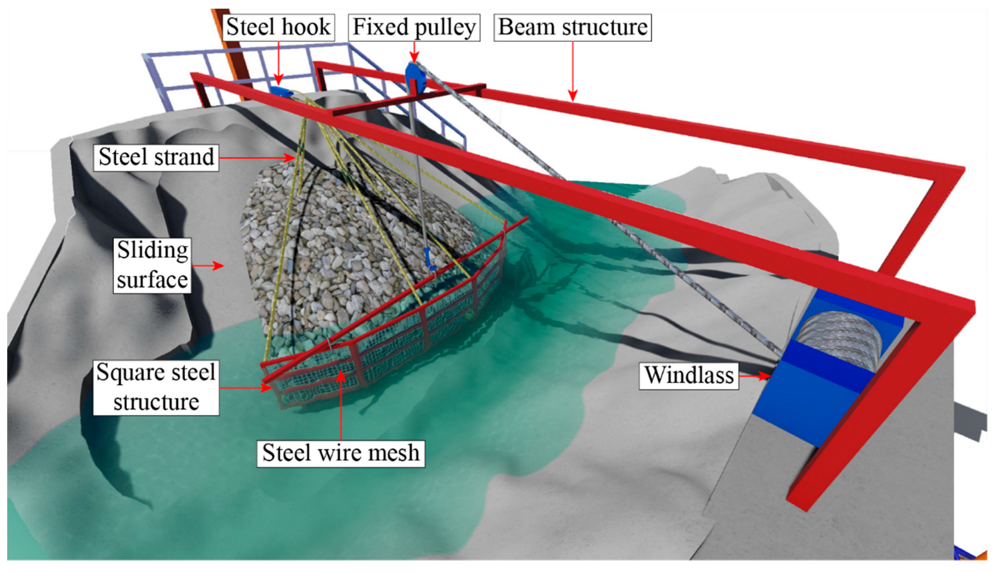
2.4. Landslide Generator Device

The landslide generator device, shown in Figure 6, uses a windlass to lift the landslide material baffle. The baffle consists of steel bars with square cross-section (4 cm width) together and covered with steel wire mesh featuring square holes (1 cm width). The baffle is connected to a steel hook by steel cables, with the hook fixed to the wall crest behind the landslide. The entire baffle can be lifted by the windlass (The TSJ-A windlass (Hebei Tianduo Crane Machinery Co., Ltd., Baoding, China)), which operates at a lifting speed of 1 m/s.

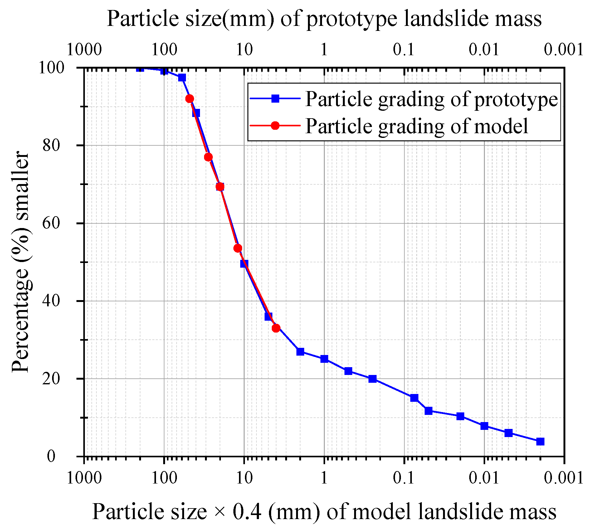
2.5. Landslide Material and Experimental Design

The landslide body consists of cobblestones (Nanjing Sanshan Pebble Factory (General Partnership), Nanjing, China), with particle sizes ranging between 1 cm and 12 cm. As shown in Figure 7, the particle size of prototype to model is 1: 2.5. Based on the relative position of the landslide mass and the water level, the landslide–water type in this experiment is classified as a partially submerged landslide, where the front edge of the landslide mass is below the water level and the rear edge is above the water level line. Five different water depths were designed in the experiment: 1.32 m, 1.242 m, 1.164 m, 1.086 m, and 1.008 m. The parameters for the physical model experiment are listed in

Table 2. Prior range and distribution of rheological parameters.

Parameters	Values	Parameters	Values	Parameters	Values
$V_s$	1.5 m3	$s$	0.5 m	$\beta$	32.3°
$M_s$	2850 kg	$l$	2.233 m	$\phi$	25°
${\rho }_s$	1.9 t/m3	$f$	0.39
$D50$	4.6 cm	$d$	1.008–1.320 m
$b_s$	4.50 m	$\alpha$	38.1°

. $V_s$ is the landslide volume, $M_s$ is the landslide mass, ${\rho }_s$ is the accumulation density of landslide, $D50$ is the particle size corresponding to a cumulative particle size distribution percentage of 50%, $b_s$ is the maximum stacking width of landslide, $s$ is the maximum stacking thickness of landslide, $l$ is the average stacking length of landslide, $f$ is the friction coefficient of sliding surface, $d$ is water depth, $\alpha$ is the sliding surface inclination angle, $\beta$ is the landslide opposite-bank inclination angle, and $\phi$ is dam surface inclination angle.

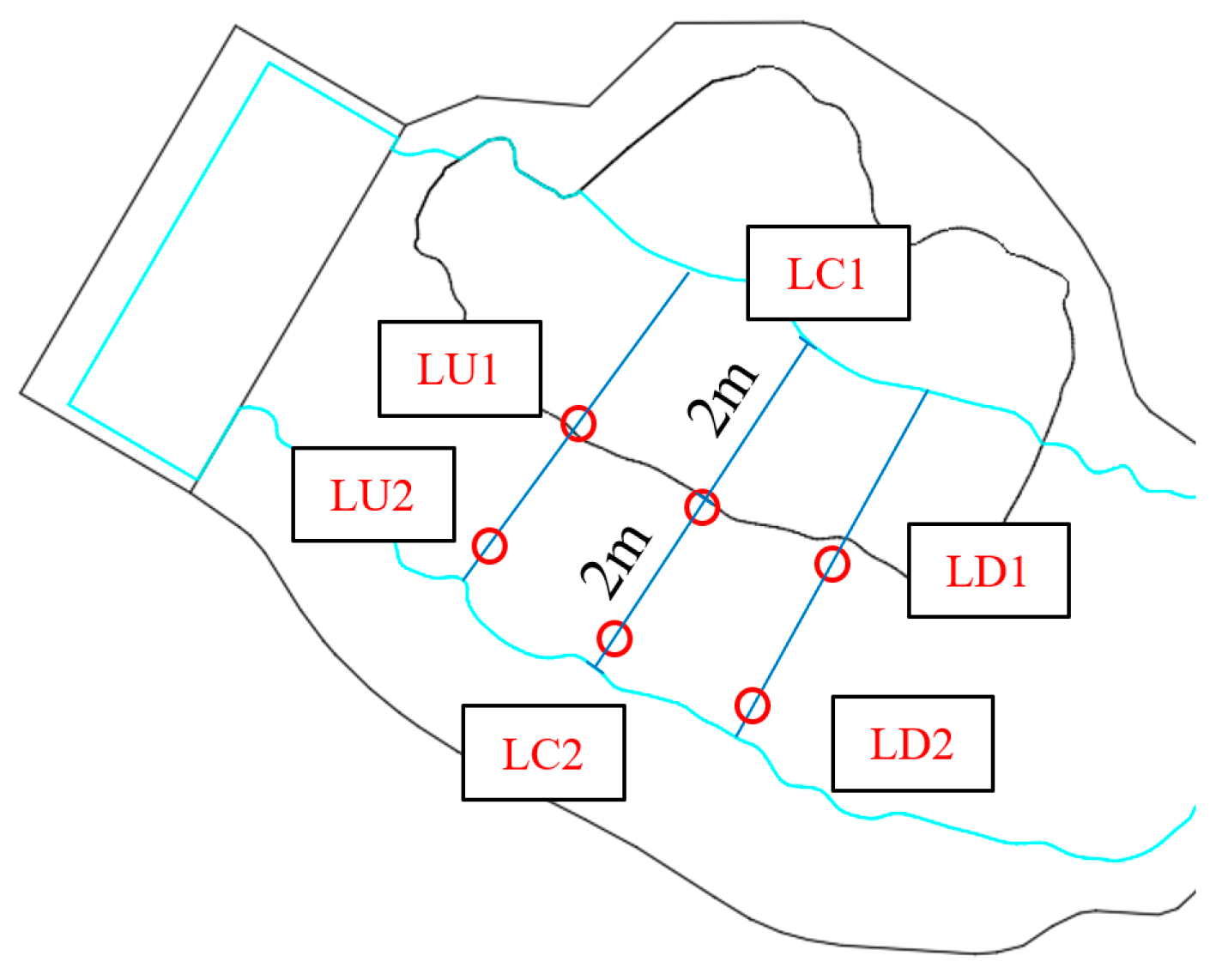
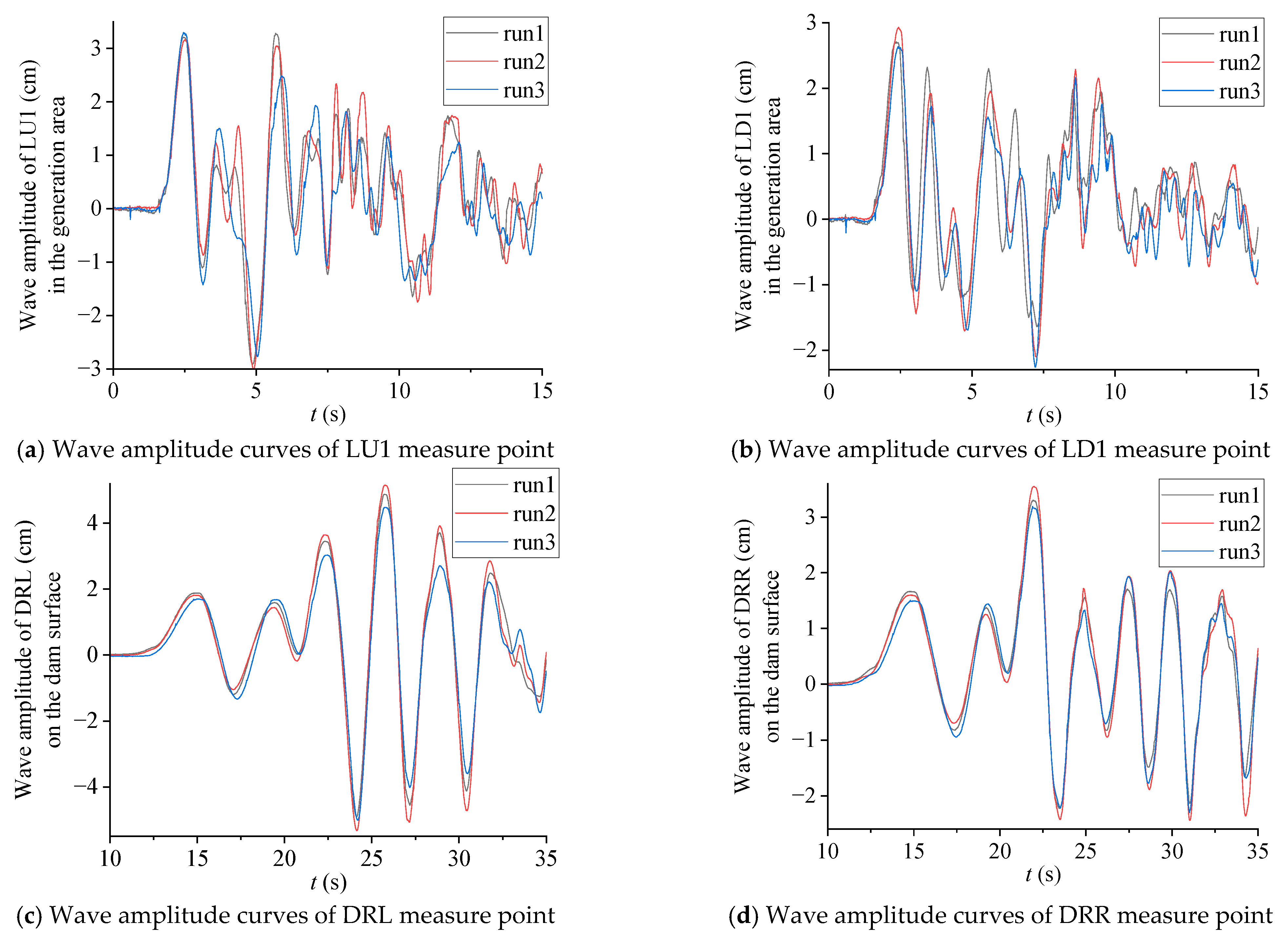
2.6. Experimental Repeatability and Error

In order to verify the repeatability of the 3D physical model experiment and measure the experimental error, three repeated experiments were conducted on the same test conditions to compare and analyze the waveform and wave amplitude data in the generation area and the dam area. In the three repeated test conditions, the layout of wave altimeter rods in the landslide area is different from that in Figure 5, as shown in Figure 8.

In the three repeated experiments, wave amplitude waveforms in the generation area and the dam area are shown in Figure 9. The consistency of the wave amplitude waveforms in the landslide area was slightly poor in the three repeated experiments, which was due to the slight changes in the geometric shape of the landslide material during the artificial stacking process. The wave amplitude waveforms on the dam surface showed excellent consistency in the three repeated experiments, indicating that slight differences in wave amplitude waveforms in the landslide area have little impact on the wave amplitude waveforms in the dam area.

In order to quantitatively analyze the differences in data obtained from the three repeated experiments and measure the data error of the 3D physical model experiment in this article, it is assumed that the mean value ($\overline{x}=(x_1+x_2+x_3)/3$) of the data values (${x=[x}_1,x_2,x_3]$) obtained from three repeated experiments at the same measuring point is the true experimental value. The difference between the experimental data value $x$ and the true experimental value $\overline{x}$ is set as the experimental error ($∆=|x-\overline{x}|$), and the maximum experimental error is set as ${∆}_{max}=|x-\overline{x}{|}_{max}$. The maximum error percentage for the experiment is set to ${∆}_{max}/\overline{x}=|x-\overline{x}{|}_{max}/\overline{x}$. The calculation results of experimental errors are shown in

Table 3. Experimental errors based on three repeated experiments.

Measure	${\mathit{H}}_1$ (cm)			${∆}_{\mathit{m}\mathit{a}\mathit{x}}$	$\frac{{∆}_{\mathit{m}\mathit{a}\mathit{x}}}{\overline{\mathit{x}}}$ (%)
Point	run1	run2	run3	(cm)
LD1	3.79	4.38	3.73	0.41	10.33
LD2	7.62	8.72	7.60	0.74	9.28
DRL	3.07	2.85	3.03	0.13	4.35
DRR	2.48	2.29	2.45	0.11	4.71

. The maximum error of wave amplitude in the generation area is less than 10.33%, and the maximum error of wave amplitude in the dam area is less than 4.71%.

3. Results

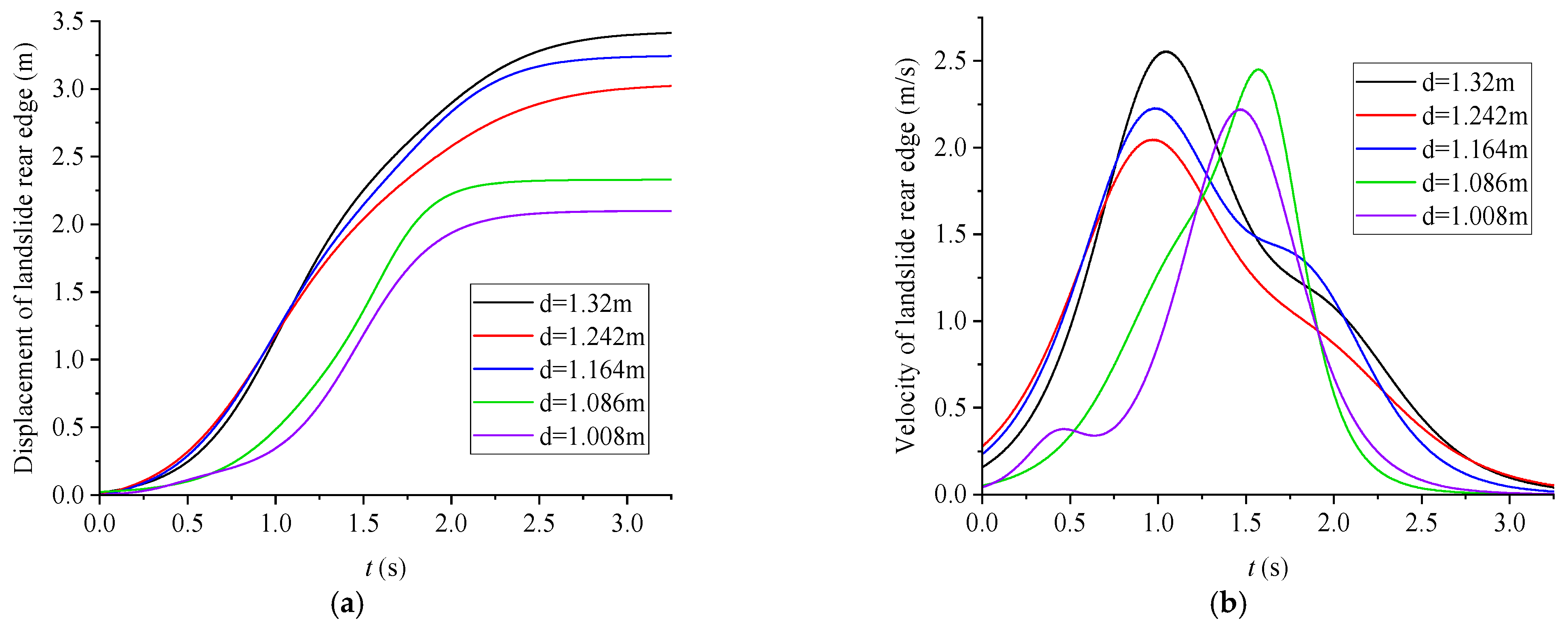
3.1. Landslide Movement

The landslide generator operates by lifting the baffle at the front edge of the landslide mass. As the baffle is lifted, the landslide material slides downward along the sliding surface from the gap where the baffle is raised. As shown in Figure 10, with a decrease in water depth, the maximum displacement of the rear edge of the landslide mass shows a decreasing trend. This is attributed to the significant frictional force between the baffle and the granular landslide material. As the water depth decreases, the submerged volume of the landslide mass decreases, resulting in a reduction in its buoyancy. Consequently, the frictional force between the landslide mass and the baffle increases, causing the lifting speed of the baffle slowing down. As shown in Figure 10b, during the sliding process, the maximum velocity at the rear edge of the landslide mass typically ranges from 2.05 m/s to 2.56 m/s, and its mean value is 2.30 m/s. According to the similarity theory, the maximum velocity at the rear edge of a real engineering landslide is 28.99 m/s to 36.20 m/s. The expected maximum speed of the engineering landslide is 24.27 m/s to 39.74 m/s, and the test speed is within this range.

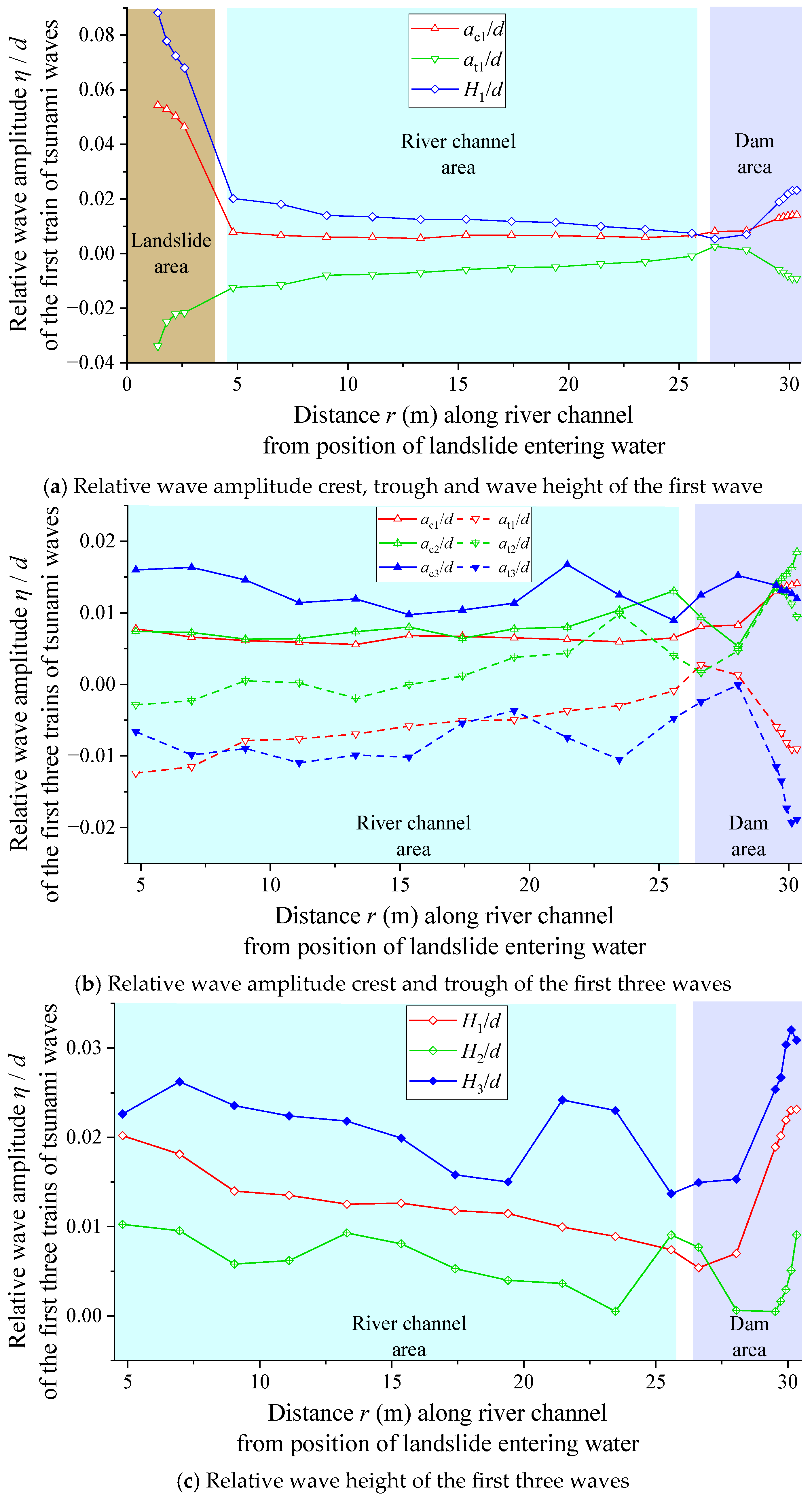
3.2. Impulse Wave Characteristics in the Generation Area

Due to the similar waveform characteristics of LIIWs under different water depth conditions, data collected at a water depth of 1.32 m is used for the following waveform characteristic analysis. When water depth is 1.32 m, the water surface width at the sliding axis is $b_w$ = 4.0 m, and four wave altimeter rods are arranged along the sliding axis. The position of the landslide entering the water is taken as the origin (x = 0 m), with four wave altimeter rods located at L1 (x = 1.4 m), L2 (x = 1.8 m), L3 (x = 2.2 m), and L4 (x = 2.6 m). Additionally, one run-up wave altimeter rod, LR1, is positioned at x = 4.0 m on the opposite bank.

Due to the small initial velocity and limited initial volume of the landslide mass in the water, the partially submerged landslide does not generate air cavities or splashing waves. During the process of the landslide mass entering the water, impact energy is primarily concentrated along the sliding axis. The maximum amplitude of the waves in the generation area occurs at the first wave crest, and the wave amplitude gradually decreases as the distance from the sliding axis increases. Because of the narrow water surface width between the two banks, when the second wave reaches the center of the water surface along the sliding axis, it interferes with the first reflected wave from the opposite bank, causing a decrease in the amplitude of the second wave and waveform fusion, as shown in Figure 11.

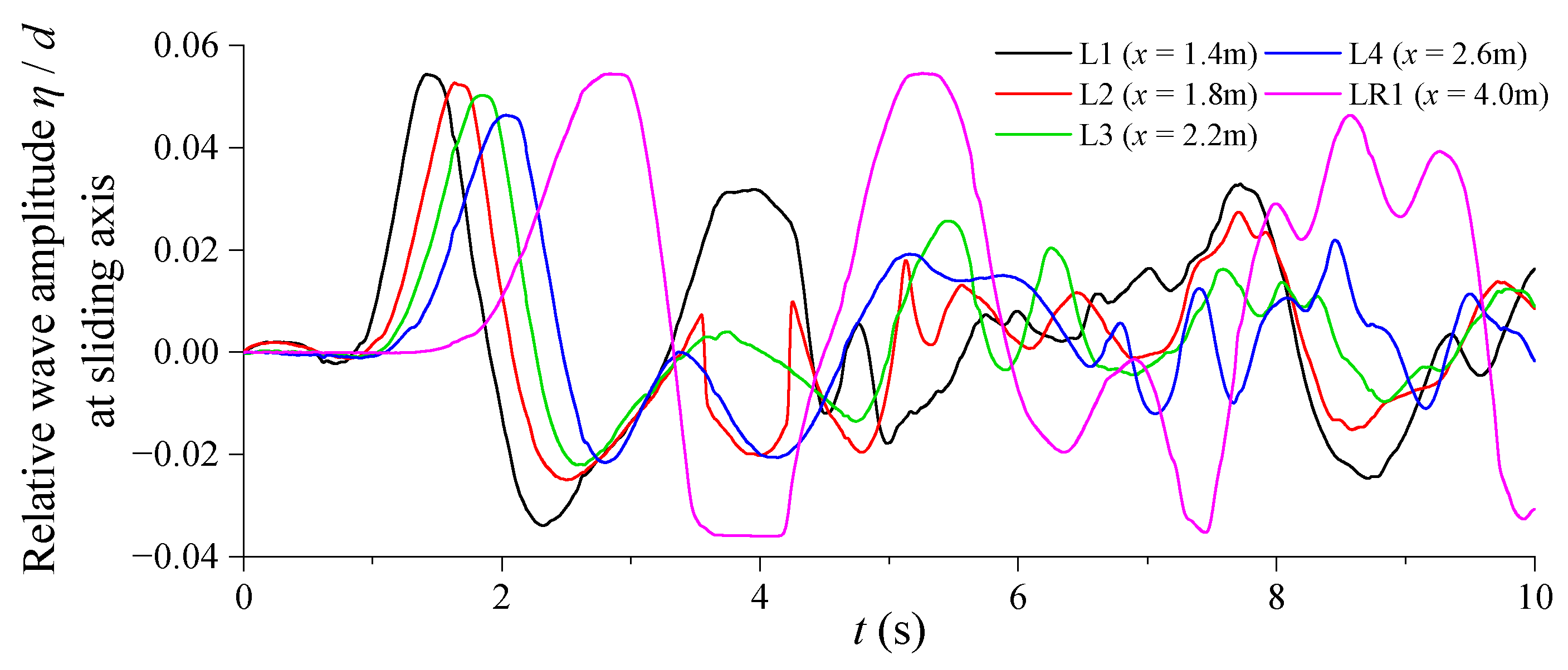
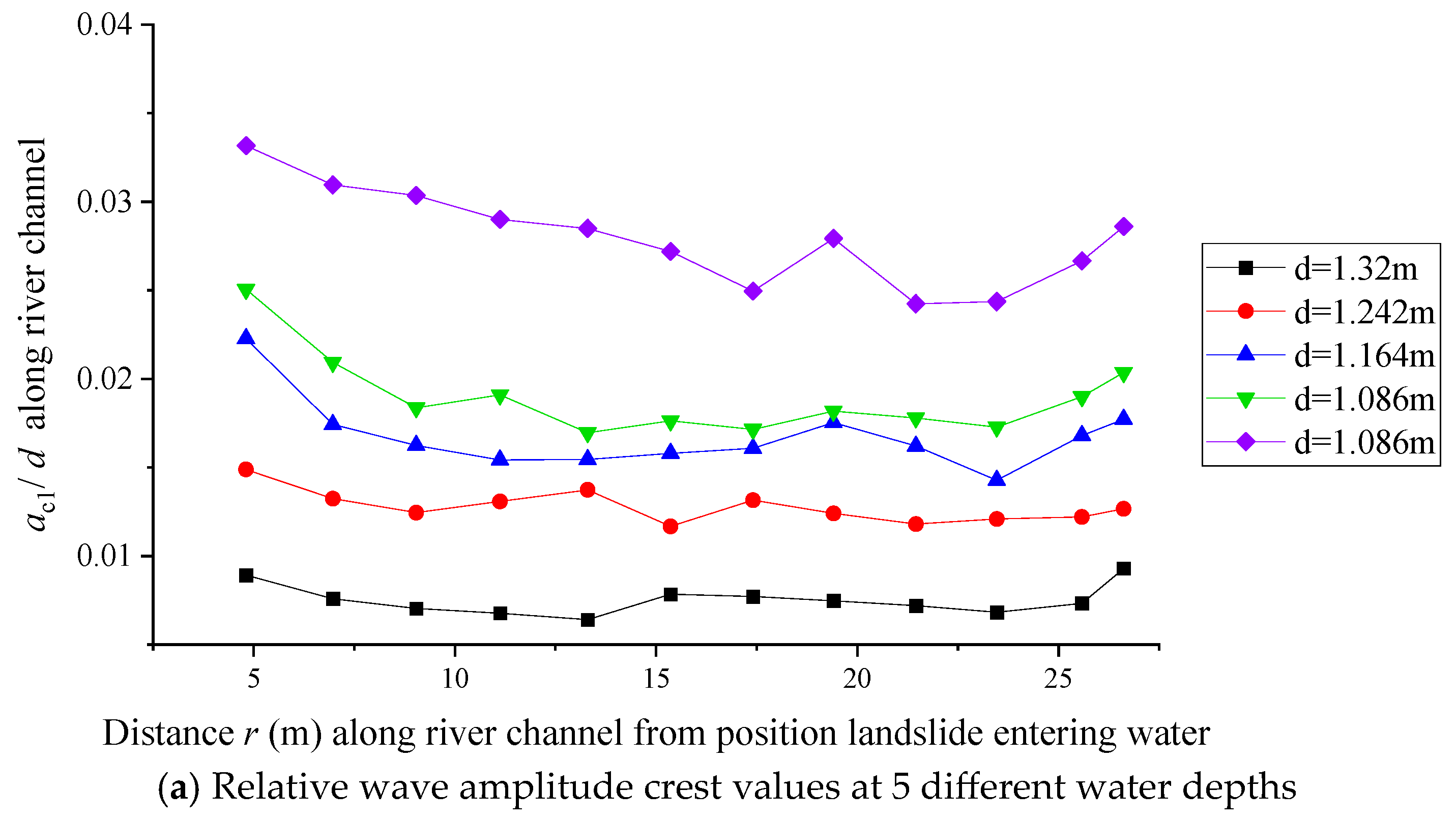
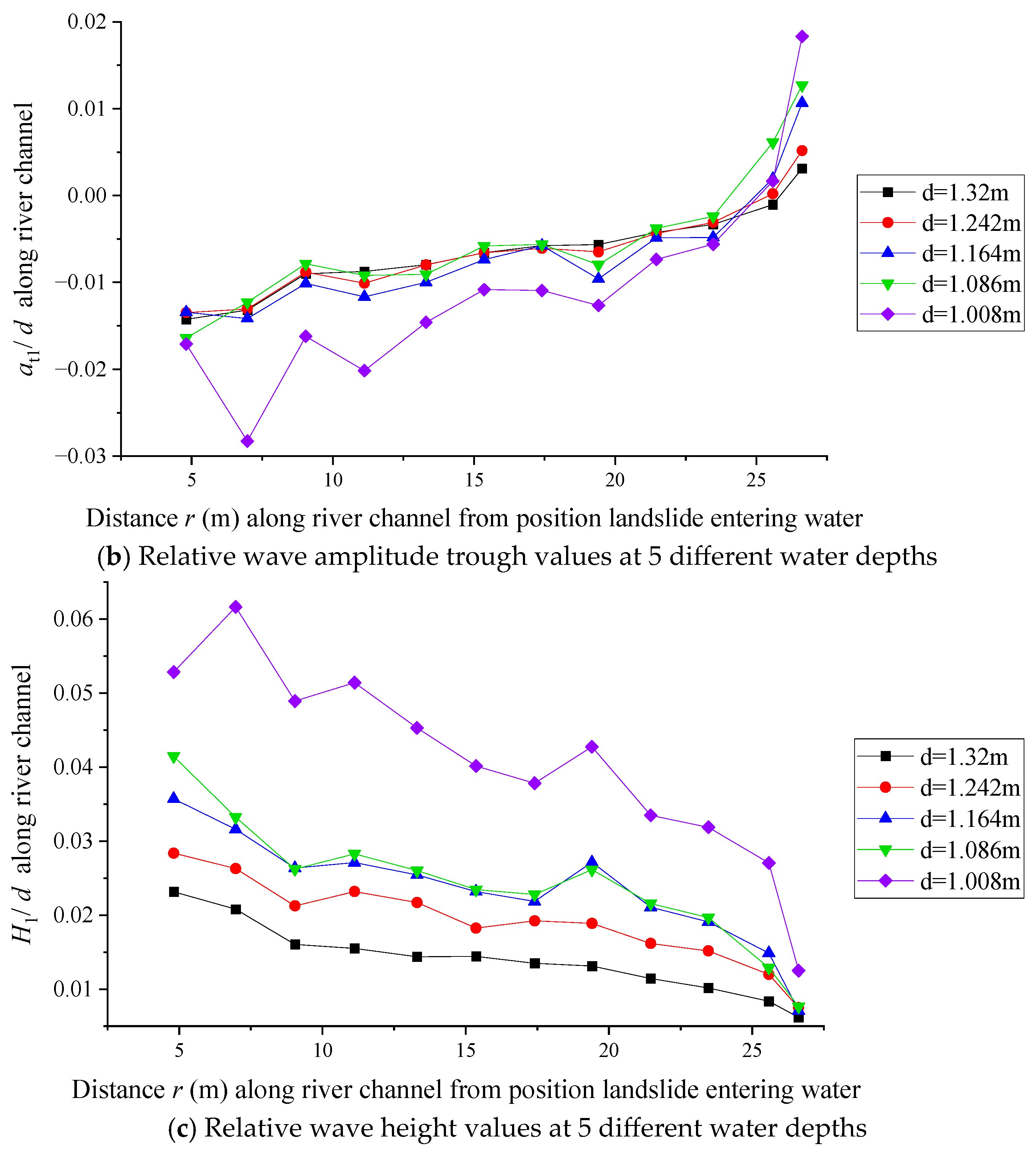
3.3. Impulse Wave Characteristics in the River Channel Propagation Area

As the angle between the direction of wave propagation and the sliding axis increases, the impact energy of the landslide mass decreases. Since the direction of the river channel is perpendicular to the sliding axis, when impulse waves enter the river channel from the generation area, wave amplitudes attenuate significantly, as shown in Figure 12a. For the first wave altimeter rod in river channel area (RC1, r = 4.81 m, θ = 79 ± 5°), and the wave altimeter rod at the center of the water surface width along the sliding axis in the generation area (L3, r = 2.2 m, θ = 0°), the amplitude attenuation rate of the first crest, calculated based on the recorded data, is given as follows.

$$\begin{array}{c}1-a_{c1,RC1}/a_{c1,L3}=84.5\%\end{array}$$

(4)

After impulse waves enter the river channel, irregular waveforms from the generation area gradually merge and become regular as propagation distances increase. Additionally, continuous oscillation of the water body between the two banks provides energy for subsequent wave trains in the river channel. The maximum wave amplitude in the river channel occurs at the third train.

Throughout the entire propagation process, the wave amplitude crests ($a_{c1}$) of the first wave remain basically unchanged, while the wave amplitude troughs ($a_{t1}$) of the first wave steadily change as the propagation distance increases, as shown in Figure 12b,c. The wave amplitude ($a_{c3}$), wave trough ($a_{t3}$), and the wave height ($H_3$) of the third wave are the maximum within the first three impulse waves. However, due to the complex terrain of the reservoir river channel, the wave amplitude may suddenly increase at certain terrain locations, especially for the third wave. This complex terrain leads to waveform fusion between the second and third wave at specific terrain locations and during the run-up process along the dam surface (Figure 13), resulting in the disappearance of the second wave trough. Notably, during the run-up process along the dam surface, the second wave crest gradually increases, while the third wave crest gradually decreases. Due to the fusion with the third wave, the second wave exhibits irregular variations in amplitude during propagation, as shown in Figure 12b,c.

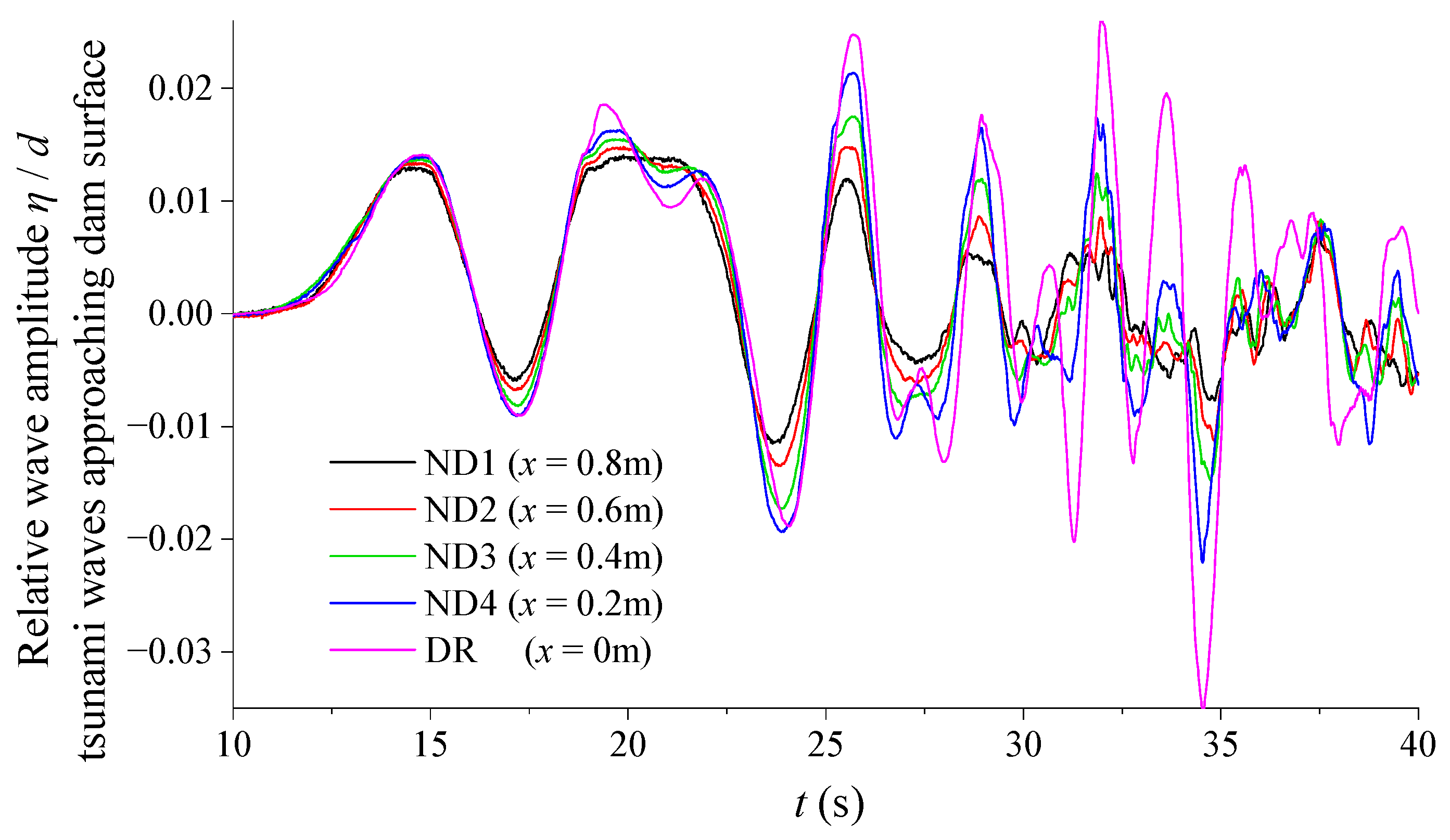
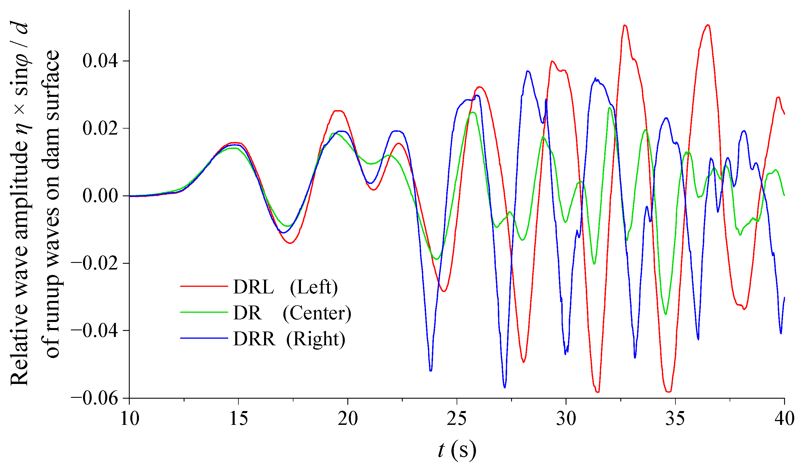
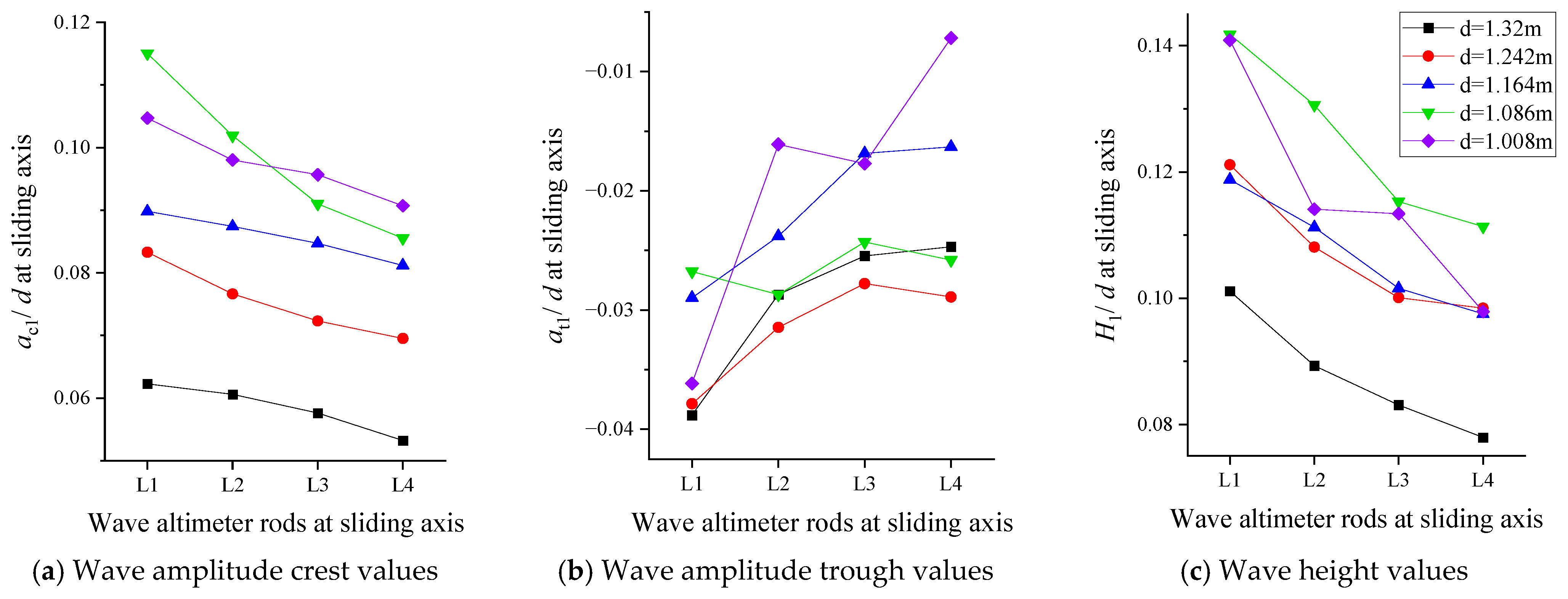
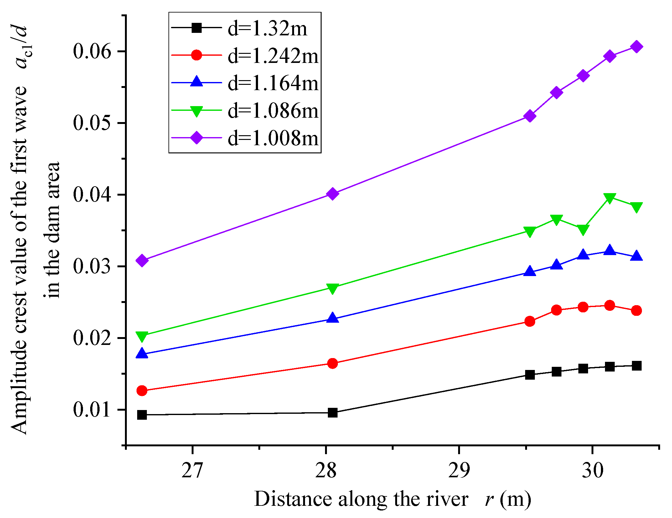
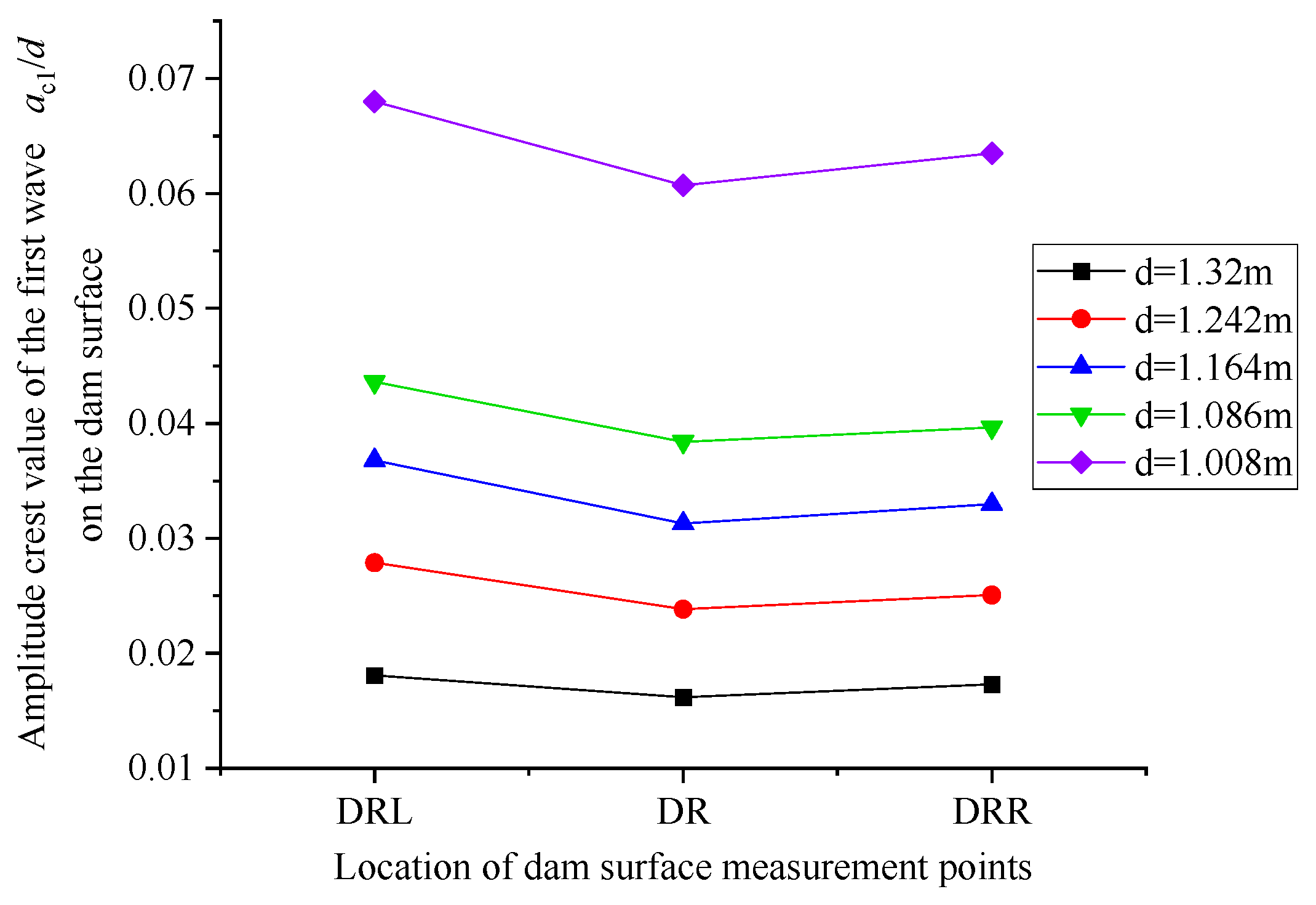
3.4. Impulse Wave Characteristics in the Dam Area and Run-Up on the Dam Surface

Let the point of intersection between the central axis of dam surface and the water surface be the origin (x = 0 m). The waveforms of the LIIWs approaching the dam surface are recorded by four wave altimeter rods in front of the dam surface: ND1 (x = 0.8 m), ND2 (x = 0.6 m), ND3 (x = 0.4 m), and ND4 (x = 0.2 m), as shown in Figure 5. The waveforms of the LIIWs run-up and drawdown along the dam surface are recorded by three wave altimeter rods: DRL (left bank of the dam surface), DR (central axis of the dam surface), and DRR (right bank of the dam surface).

As the LIIWs approach the dam surface, the cross-sectional area of the water body gradually decreases due to the inclination of the dam surface, causing the wave amplitude to gradually increase (Figure 13). Notably, due to the fusion of the second and third waves, the second wave trough disappears, and the third wave crest gradually decreases.

Due to asymmetry of terrain in the dam area, LIIWs do not rise and fall uniformly along the width of the dam surface during run-up and drawdown. Starting from the fourth wave train, a differential run-up is observed between the left and right sides of the dam surface, as shown in Figure 14. As the oscillation progresses, the run-up amplitude on the dam surface further increases. When the run-up wave crest of the left bank coincides with drawdown wave trough on the right bank, the run-up amplitude on the dam surface reaches its peak and then gradually decreases. Due to the sharply angled terrain on both banks of the dam surface, where impact energy is more concentrated, the amplitudes of the run-up and drawdown waves on the left and right sides of the dam surface are greater than those in the center of the dam surface.

4. Discussion

During the construction of a dam, a cofferdam in front of the dam is usually used to intercept the water flow and simultaneously store water, and the water level of the reservoir and the height of the water-retaining curtain increase synchronously with the height of the dam construction. If a LIIW disaster occurs during the construction of the dam, the safety of the dam construction can only be guaranteed when the wave amplitude height of the LIIWs propagating to the front of the dam are less than the height of the cofferdam. When at the maximum water level of the reservoir, if a LIIW disaster occurs, the LIIWs will propagate to the dam and run up along the dam surface. Only when the LIIWs do not overflow the dam can the safe operation of the reservoir be ensured.

Previous studies have shown that the factors affecting the height of LIIWs primarily include the volume and sliding speed of landslide mass and water depth. During the dam construction period and operation period of the reservoir, the amplitude of LIIWs in front of and on the dam surface affects the safety of reservoir construction and operation. Therefore, this study mainly focuses on changes in water depth and designs five model experiments at different water depths, with particular emphasis on analyzing the impact of water depth on LIIWs.

The lowest water depth set in the model experiment corresponds to the lowest water level during the water level scheduling process of the engineering reservoir, and the highest water depth set in the model experiment corresponds to the highest water level during the water level scheduling process of the engineering reservoir. Linear interpolation of three water depths in the middle corresponds to the filling heights of three stages during the dam construction period.

4.1. The Influence of Different Water Depths on the Impulse Wave Characteristics in the Generation Area

As shown in Figure 15, data from the four wave altimeter rods (L1~L4) at the sliding axis indicate that wave amplitude increases as the water depth decreases. The attenuation of the first wave crest $a_{c1}$ at different water depths shows a good regularity with distance. However, the regularity of the first wave trough $a_{t1}$ attenuation is poor, which is due to the waveform confusion caused by the reflected waves on the opposite bank of the landslide, affecting the first wave trough $a_{t1}$ values of some measuring points. Affected by the first wave trough $a_{t1}$, the regularity of the first wave height $H_1=a_{c1}-a_{t1}$ attenuation is also poor.

When the water depth ($d$) is different, the width of the water surface ($b_w$) at the sliding axis also changes. The distances between the four wave altimeter rods (L1~L4) and the position where the landslide enters the water are shown in

Table 4. Distance $r$ between the wave altimeter rods and the position of landslide entering water at the sliding axis at different water depths.

d (m)	bw (m)	r (m)
		L1	L2	L3	L4
1.32	4.0	1.4	1.8	2.2	2.6
1.242	3.8	1.3	1.7	2.1	2.5
1.164	3.6	1.2	1.6	2.0	2.4
1.086	3.4	1.1	1.5	1.9	2.3
1.008	3.2	1.0	1.4	1.8	2.2

.

In order to quantitatively analyze the attenuation law of the first wave crest values in the generation area, the dimensionless formula method widely used by scholars was adopted to fit the experimental data. In the experiments in this study, the only variable is water depth ($d$). According to the studies of other researchers, dimensionless parameters related to water depth ($d$) include $F=v_s/(gd{)}^{0.5}$, $V_{\mathrm{s}}/d^3$, and ${V_{\mathrm{s}}/b}_s{d}^2$. The range of dimensionless parameter values is shown below.

$$\begin{array}{c}{\displaystyle \frac{a_{c1}\left(d,r\right)}{d}}=k_1{F}^{k_2}{\left({\displaystyle \frac{V_s}{{b_{s}d}^2}}\right)}^{k_3}{\left({\displaystyle \frac{r}{d}}\right)}^{k_4}\end{array}$$

(5)

Based on Equation (5), the wave amplitude crest data in Figure 15a was fitted, and the values of parameters $k_1$, $k_2$, $k_3$, and $k_4$ were obtained as 0.30, 0.26, 0.78, and −0.25. Substituting the parameters into Equation (5), the following equation is obtained.

$$\begin{array}{c}{\displaystyle \frac{a_{c1}\left(d,r\right)}{d}}=0.3F^{0.26}{\left({\displaystyle \frac{V_s}{{b_{s}d}^2}}\right)}^{0.78}{\left({\displaystyle \frac{r}{d}}\right)}^{-0.25}\end{array}$$

(6)

Comparison between empirical formula-predicted values and experimental data is shown in Figure 16; the effectiveness of the empirical formula for the attenuation of the first wave crest $a_{c1}$ along the sliding axis is 88%.

The experimental data from this article was substituted into the empirical formulas of other researchers and compared with the empirical formula proposed in this article, as shown in Figure 17. In Figure 17, SA represents subaerial landslide, PS represents partially submerged landslide, B represents block material, and G represents granular material. Heller (2013) [14], Ataie-Ashtiani (2008) [39], Heller (2011) [25], Heller (2015) [48], Panizzo (2005) [3], Mohammed (2012) [51], the fitting formulas of these references are cited in this article.

It can be seen that the calculation results of two-dimensional experimental empirical formulas are greater than those of three-dimensional experiments. This is due to the constraint of the side wall of the two-dimensional experimental water tank, which concentrates the energy of the LIIWs and causes the amplitude of the LIIWs in the two-dimensional experiment to be greater than that in the three-dimensional experiments. There are still significant differences in the calculation results of the empirical formulas among three-dimensional experiments. This phenomenon indicates that there are differences in the attenuation law of LIIWs under different landslide morphology and engineering terrains, and it is difficult for the empirical formulas proposed in existing research to have universality. It is necessary to establish a similar physical model based on the engineering terrain when estimating the wave amplitude of LIIWs of specific engineering.

4.2. The Influence of Different Water Depths on the Impulse Wave Characteristics in the River Channel Propagation Area

As shown in Figure 18, data from the 12 wave altimeter rods (RC1~RC11, and D1) along the central axis of the river channel indicate that the wave amplitude increases as water depth decreases. In the range of r = 5~8 m, the rate of decay of $a_{c1}$ increases as the water depth decreases. In the range of r = 8~24 m, the value of $a_{c1}$ remains relatively unchanged. In the range of r = 24~27 m, the value of $a_{c1}$ begins to increase. The value of $a_{t1}$ remains consistent under different water depth conditions. It is worth noting that when r = 24~27 m, the value of $a_{t1}$ changes from negative to positive and begins to increase rapidly. The value of $H_1$ decays rapidly in the range of r = 5~8 m, decays more slowly in the range of r = 8~24 m, and decays rapidly again in the range of r = 24~27 m. At certain locations in the river channel, the amplitude of swell waves increases abnormally with distance, and the wave height $H_1$ exhibits different attenuation rates at different positions. These observations indicate that the terrain of the river channel significantly influences the attenuation of LIIWs’ amplitude. Furthermore, conventional formulas cannot accurately fit the attenuation law of wave amplitude in such complex river channel terrains.

4.3. The Influence of Different Water Depths on the Impulse Wave Characteristics in the Dam Area

As shown in Figure 19, data from the seven wave altimeter rods (D1, D2, ND1~ND4, DR) along the central axis of the dam surface indicate that the wave amplitude crest of the first wave increases as water depth decreases. As the impulse waves run up along the inclined dam surface, the amplitude crest value gradually increases. The increase speed of wave amplitude near the dam surface slows down, as the resistance of the dam surface to the water gradually increases as impulse waves run up. For the physical model presented in this article, the maximum wave run-up height is observed on the left bank of the dam surface. Figure 20 shows the wave run-up height on the dam surface at different water depths.

The amplitude crest value of the first wave $a_{c1}$ at measurement point D1 at the foot of the dam is defined as the maximum wave amplitude $a_{d,max}$ in front of the dam, $a_{d,max}=a_{c1}{|}_{\mathrm{D}1}$. The amplitude crest value of the first wave $a_{c1}\times sin\phi$ at measurement point DRL at the left bank of the dam surface is defined as the maximum wave amplitude $R_{d,max}$ on the dam surface, $R_{d,max}=a_{c1}{|}_{\mathrm{D}\mathrm{R}\mathrm{L}}\times sin\phi$. The empirical formula for the maximum run-up height on the dam surface is as follows.

$$\begin{array}{c}{\displaystyle \frac{R_{d,max}\left(d\right)}{d}}=k_1{F}^{k_2}{\left({\displaystyle \frac{V_s}{{b_{s}d}^2}}\right)}^{k_3}{\left({\displaystyle \frac{a_{d,max}}{d}}\right)}^{k_4}\end{array}$$

(7)

Based on Equation (7), the wave amplitude crest data in Figure 19 was fitted, and the values of parameters $k_1$, $k_2$, $k_3$, and $k_4$ were obtained as 0.02, −2, 0.53, and 1.05. Substituting the parameters into Equation (7), the following equation is obtained.

$$\begin{array}{c}{\displaystyle \frac{R_{d,max}\left(d\right)}{d}}=0.02F^{-2}{\left({\displaystyle \frac{V_s}{{b_{s}d}^2}}\right)}^{0.53}{\left({\displaystyle \frac{a_{d,max}}{d}}\right)}^{1.05}\end{array}$$

(8)

Comparison between empirical formula-predicted values and experimental data is shown in Figure 21; the effectiveness of the empirical formula for maximum run-up height on the dam surface is 95%.

4.4. Prediction of Impulse Wave of Potential Landslide in Real Engineering Based on Physical Model Experiment

Based on the results of similar physical model experiments and similarity theory, the amplitude crest values of the LIIWs for the real engineering dimensions are shown in

Table 5. The amplitude crest values of the LIIWs for the real engineering dimensions.

Water Level	Altitude (m)	${\mathit{a}}_{\mathit{c}1}{|}_{\mathit{L}\mathit{C}}$ (m)	${\mathit{a}}_{\mathit{c}1}{|}_{\mathit{D}\mathit{T}}$ (m)	${\mathit{a}}_{\mathit{c}1~3}{|}_{\mathit{D}\mathit{T}}$ (m)	${\mathit{R}}_{\mathit{c}1}{|}_{\mathit{D}\mathit{C}}$ (m)	${\mathit{R}}_{\mathit{c}1~3}{|}_{\mathit{D}\mathit{C}}$ (m)	${\mathit{R}}_{\mathit{c}1}{|}_{\mathit{D},\mathit{m}\mathit{a}\mathit{x}}$ (m)	${\mathit{R}}_{\mathit{c}1~3}{|}_{\mathit{D},\mathit{m}\mathit{a}\mathit{x}}$ (m)	${\mathit{R}}_{\mathit{c}1~6}{|}_{\mathit{D},\mathit{m}\mathit{a}\mathit{x}}$ (m)
Maximum operating	2895	17.49	2.45	3.79	4.28	5.62	4.77	7.63	15.34
Construction period	2879.4	18.20	3.27	5.63	5.92	6.60	6.93	9.41	16.05
	2863.8	18.98	4.13	7.61	7.29	11.25	8.56	12.06	17.85
	2848.2	19.85	4.42	7.76	8.33	13.75	9.47	15.71	16.55
	2832.6	20.82	6.22	8.93	12.24	17.30	13.71	20.36	20.36

. $a_{c1}{|}_{LC}$ is the amplitude crest value of the first wave at the center of the water surface at the sliding axis of the landslide (based on the calculation result of Equation (6)), $a_{c1}{|}_{DT}$ is the amplitude crest value of the first wave at the dam foot, $a_{c1~3}{|}_{DT}$ is the maximum amplitude crest value of the first three waves at the dam foot, $R_{c1}{|}_{DC}$ is the amplitude crest vertical height of the first wave run-up along the dam surface at the center of dam surface, $R_{c1~3}{|}_{DC}$ is the maximum amplitude crest vertical height of the first three waves’ run-up along the dam surface at the center of dam surface, $R_{c1}{|}_{D,max}$ is the maximum amplitude crest vertical height of the first wave run-up along the dam surface, $R_{c1~3}{|}_{D,max}$ is the maximum amplitude crest vertical height run-up along the dam surface of the first three waves, and $R_{c1~6}{|}_{D,max}$ is the maximum amplitude crest vertical height run-up along the dam surface of the first six waves.

During the construction of a dam, a cofferdam in front of the dam is usually used to intercept the water flow and simultaneously store water. According to the maximum amplitude crest value of the first three waves at the dam foot, $a_{c1~3}{|}_{DT}$ in Table 5, in order to prevent potential landslide from surging over the cofferdam during dam construction, the height of the cofferdam should be at least 8.93 m above the water level.

At the maximum water level during the operation of the reservoir, when the potential landslide of 12 million cubic meters induces impulse waves that impact the dam surface, the run-up height of the impulse waves during the first three columns is less than the altitude of the dam top. However, due to the terrain of the dam area, the water on the dam surface oscillates between the two banks, causing the rising height of the LIIWs to gradually increase. At the sixth wave, the maximum run-up wave height at the angle between the dam surface and the left bank exceeds the dam top altitude by 3.34 m. To ensure the safe operation of the reservoir, it is recommended to install wave dissipating facilities at the angle between the dam surface and both banks, such as building wave dissipating steps, installing wave walls, or setting up small spillway tunnels at the angle.

5. Conclusions

A large-scale three-dimensional similar physical model was established based on the terrain data of RM reservoir. The experiments recorded and analyzed the generation and propagation laws of LIIWs in RM reservoir at five different water depths. The following conclusions can be drawn.

(1)

Partially submerged landslides will not generate splashing waves when entering the water. The maximum wave amplitude in the generation area occurs in the first wave column, and the maximum wave amplitude in the propagation area occurs in the third wave column. The wave amplitude values decrease with increasing propagation distance and increasing water depth. The water at the dam surface experiences repeated oscillations between the two banks, which cause the LIIW run-up height along the dam surface to further increase.

(2)

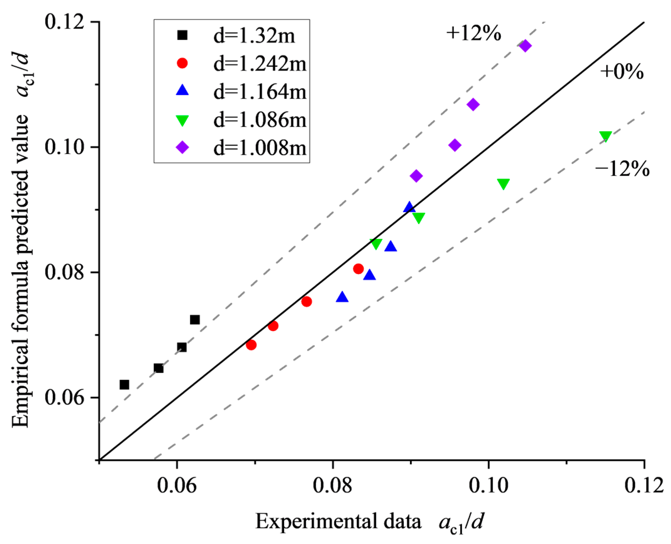
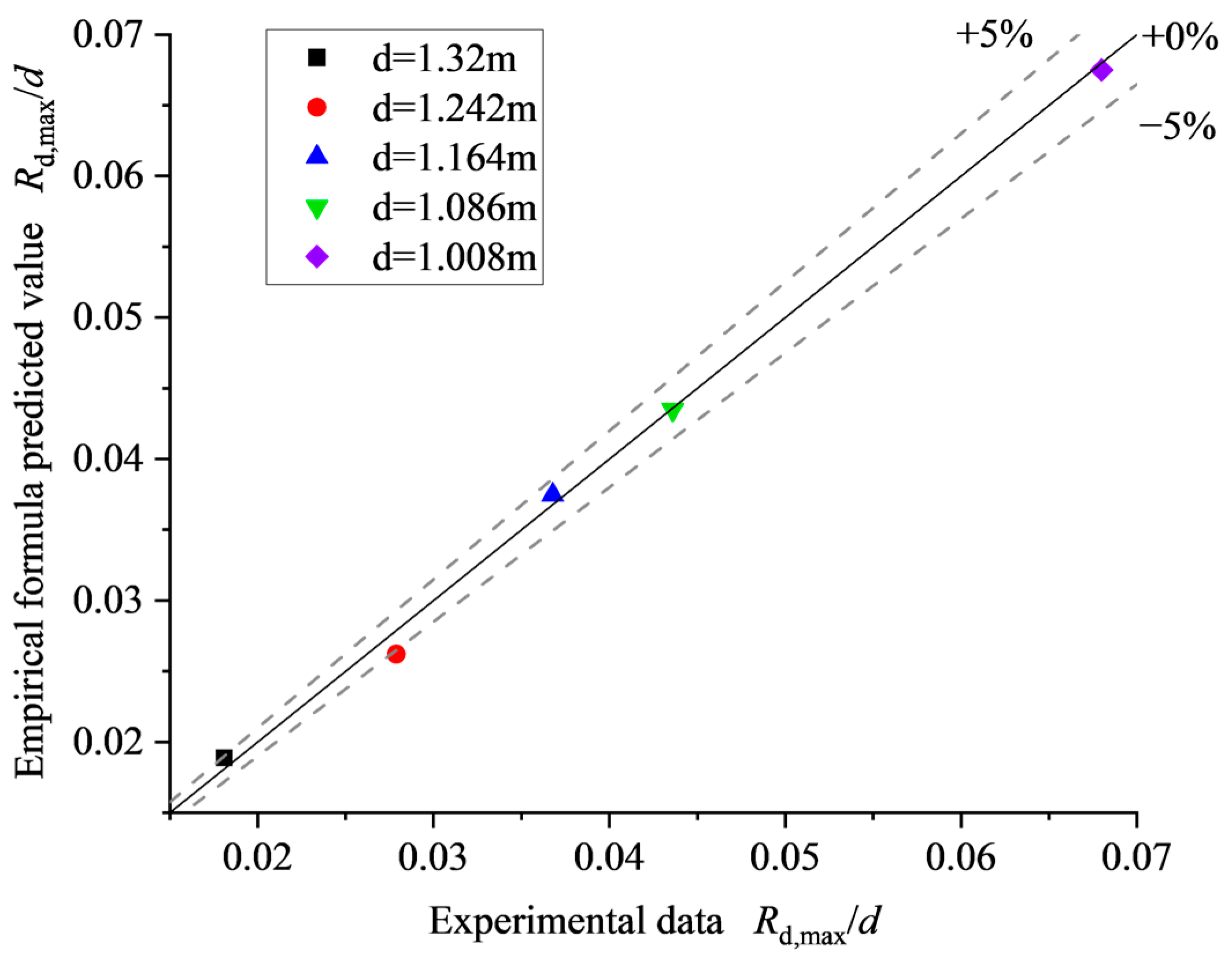
The empirical formulas of wave amplitude crest attenuation in the generation area and wave vertical run-up height on the dam surface are proposed, whose effectiveness are 88% and 95%. By comparing with empirical formulas proposed by other researchers, it was found that landslide morphology and engineering terrain have a significant impact on the attenuation law of LIIWs.

(3)

Based on experimental results, the following suggestions were proposed for the unbuilt RM reservoir project: The height of the cofferdam should be at least 8.93 m above the water level during the dam layered construction period. In order to prevent the maximum run-up wave height from exceeding the dam top altitude, it is recommended to install wave dissipating facilities at the junction between the dam surface and both banks.

The attenuation mechanism of wave amplitude during the propagation is crucial for evaluating the potential impacts of LIIW disasters in complex river terrains. Therefore, further research is necessary to establish an empirical formula that relates wave amplitude attenuation to parameters of complex river channels, such as cross-sectional area, water surface width, and river angle. Additionally, the pressure distribution on the dam surface and its influence on the stability of the dam during impulse wave impact require further investigation in future studies.

References

1. Zhang, X.; Shuang, N.; Lu, X.; Xiong, B.; Ming, H.; Cai, Z.; Liu, X. The effect of river channel characteristics on landslide-generated waves and the dynamic water pressure of the dam surface. Water 2022, 14, 1543. [Google Scholar] [CrossRef]
2. Panizzo, A.; De Girolamo, P.; Di Risio, M.; Maistri, A.; Petaccia, A. Great landslide events in Italian artificial reservoirs. Nat. Hazards Earth Syst. Sci. 2005, 5, 733–740. [Google Scholar] [CrossRef]
3. Panizzo, A.; De Girolamo, P.; Petaccia, A. Forecasting impulse waves generated by subaerial landslides. J. Geophys. Res. 2005, 110, 2004JC002778. [Google Scholar] [CrossRef]
4. Ma, H.; Wang, H.; Xu, W.; Zhan, Z.; Wu, S.; Xie, W.-C. Numerical modeling of landslide-generated impulse waves in mountain reservoirs using a coupled DEM-SPH method. Landslides 2024, 21, 2007–2019. [Google Scholar] [CrossRef]
5. Xu, W.-J.; Dong, X.-Y. Simulation and verification of landslide tsunamis using a 3D SPH-DEM coupling method. Comput. Geotech. 2021, 129, 103803. [Google Scholar] [CrossRef]
6. Mao, J.; Zhao, L.; Di, Y.; Liu, X.; Xu, W. A resolved CFD–DEM approach for the simulation of landslides and impulse waves. Comput. Methods Appl. Mech. Eng. 2020, 359, 112750. [Google Scholar] [CrossRef]
7. Ma, H.; Wang, H.; Shi, H.; Xu, W.; Hou, J.; Wu, W.; Xie, W.-C. Probabilistic landslide-generated impulse waves estimation in mountain reservoirs, a case study. Bull. Eng. Geol. Environ. 2024, 83, 494. [Google Scholar] [CrossRef]
8. Gao, J.; Bi, W.J.; Zhang, J.; Zang, J. Numerical Investigations on Harbor Oscillations Induced by Falling Objects. China Ocean Eng. 2023, 37, 458–470. [Google Scholar] [CrossRef]
9. Gao, J.; Ma, X.; Chen, H.; Zang, J.; Dong, G. On hydrodynamic characteristics of transient harbor resonance excited by double solitary waves. Ocean Eng. 2021, 219, 108345. [Google Scholar] [CrossRef]
10. Gao, J.; Ma, X.; Zang, J.; Dong, G.; Ma, X.; Zhu, Y.; Zhou, L. Numerical investigation of harbor oscillations induced by focused transient wave groups. Coast. Eng. 2020, 158, 103670. [Google Scholar] [CrossRef]
11. Junliang, G.; Xiaojun, Z.; Li, Z.; Jun, Z.; Qiang, C.; Haoyu, D. Numerical study of harbor oscillations induced by water surface disturbances within harbors of constant depth. Ocean Dyn. 2018, 68, 1663–1681. [Google Scholar]
12. Grilli, S.T.; Shelby, M.; Kimmoun, O.; Dupont, G.; Nicolsky, D.; Ma, G.; Kirby, J.T.; Shi, F. Modeling coastal tsunami hazard from submarine mass failures: Effect of slide rheology, experimental validation, and case studies off the US east coast. Nat. Hazards 2017, 86, 353–391. [Google Scholar] [CrossRef]
13. Heinrich, P. Nonlinear water waves generated by submarine and aerial landslides. J. Waterw. Port Coast. Ocean Eng. 1992, 118, 249–266. [Google Scholar] [CrossRef]
14. Heller, V.; Spinneken, J. Improved landslide-tsunami prediction: Effects of block model parameters and slide model. J. Geophys. Res. Oceans 2013, 118, 1489–1507. [Google Scholar] [CrossRef]
15. Kamphuis, J.W.; Bowering, R.J. Impulse waves generated by landslides. In Proceedings of the Coastal Engineering Proceedings, Washington, DC, USA, 17 September 1970; Volume 35, pp. 575–588. [Google Scholar]
16. Noda, E. Water waves generated by landslides. J. Waterw. Harb. Coast. Eng. Div. 1970, 96, 835–855. [Google Scholar] [CrossRef]
17. Panizzo, A.; Bellotti, G.; De Girolamo, P. Application of wavelet transform analysis to landslide generated waves. Coast. Eng. 2002, 44, 321–338. [Google Scholar] [CrossRef]
18. Sælevik, G.; Jensen, A.; Pedersen, G. Experimental investigation of impact generated tsunami; related to a potential rock slide, western Norway. Coast. Eng. 2009, 56, 897–906. [Google Scholar] [CrossRef]
19. Walder, J.S.; Watts, P.; Sorensen, O.E.; Janssen, K. Tsunamis generated by subaerial mass flows. J. Geophys. Res. 2003, 108, 2001JB000707. [Google Scholar] [CrossRef]
20. Watts, P. Tsunami features of solid block underwater landslides. J. Waterw. Port Coast. Ocean Eng. 2000, 126, 144–152. [Google Scholar] [CrossRef]
21. Fritz, H.; Hager, W.; Minor, H.-E. Lituya bay case: Rockslide impact and wave run-up. Sci. Tsunami Hazards 2001, 19, 3–19. [Google Scholar]
22. Fritz, H.M.; Hager, W.H.; Minor, H.-E. Near field characteristics of landslide generated impulse waves. J. Waterw. Port Coast. Ocean Eng. 2004, 130, 287–302. [Google Scholar] [CrossRef]
23. Zweifel, A.; Hager, W.H.; Minor, H.-E. Plane impulse waves in reservoirs. J. Waterw. Port Coast. Ocean Eng. 2006, 132, 358–368. [Google Scholar] [CrossRef]
24. Heller, V.; Hager, W.H.; Minor, H.-E. Scale effects in subaerial landslide generated impulse waves. Exp. Fluids 2008, 44, 691–703. [Google Scholar] [CrossRef]
25. Heller, V.; Hager, W.H. Wave types of landslide generated impulse waves. Ocean Eng. 2011, 38, 630–640. [Google Scholar] [CrossRef]
26. Fuchs, H.; Winz, E.; Hager, W.H. Underwater landslide characteristics from 2D laboratory modeling. J. Waterw. Port Coast. Ocean Eng. 2013, 139, 480–488. [Google Scholar] [CrossRef]
27. Viroulet, S.; Sauret, A.; Kimmoun, O. Tsunami generated by a granular collapse down a rough inclined plane. Europhys. Lett. 2014, 105, 34004. [Google Scholar] [CrossRef]
28. Evers, F.; Hager, W. Impulse wave generation: Comparison of free granular with mesh-packed slides. J. Mar. Sci. Eng. 2015, 3, 100–110. [Google Scholar] [CrossRef]
29. Miller, G.S.; Take, W.A.; Mulligan, R.P.; McDougall, S. Tsunamis generated by long and thin granular landslides in a large flume. J. Geophys. Res. Oceans 2017, 122, 653–668. [Google Scholar] [CrossRef]
30. Cabrera, M.A.; Pinzon, G.; Take, W.A.; Mulligan, R.P. Wave generation across a continuum of landslide conditions from the collapse of partially submerged to fully submerged granular columns. J. Geophys. Res. Oceans 2020, 125, e2020JC016465. [Google Scholar] [CrossRef]
31. Huang, B.; Zhang, Q.; Wang, J.; Luo, C.; Chen, X.; Chen, L. Experimental study on impulse waves generated by gravitational collapse of rectangular granular piles. Phys. Fluids 2020, 32, 033301. [Google Scholar] [CrossRef]
32. Robbe-Saule, M.; Morize, C.; Henaff, R.; Bertho, Y.; Sauret, A.; Gondret, P. Experimental investigation of tsunami waves generated by granular collapse into water. J. Fluid Mech. 2021, 907, A11. [Google Scholar] [CrossRef]
33. Takabatake, T.; Mäll, M.; Han, D.C.; Inagaki, N.; Kisizaki, D.; Esteban, M.; Shibayama, T. Physical modeling of tsunamis generated by subaerial, partially submerged, and submarine landslides. Coast. Eng. J. 2020, 62, 582–601. [Google Scholar] [CrossRef]
34. Tang, G.; Lu, L.; Teng, Y.; Zhang, Z.; Xie, Z. Impulse waves generated by subaerial landslides of combined block mass and granular material. Coast. Eng. 2018, 141, 68–85. [Google Scholar] [CrossRef]
35. Meng, Z. Experimental study on impulse waves generated by a viscoplastic material at laboratory scale. Landslides 2018, 15, 1173–1182. [Google Scholar] [CrossRef]
36. Bullard, G.K.; Mulligan, R.P.; Carreira, A.; Take, W.A. Experimental analysis of tsunamis generated by the impact of landslides with high mobility. Coast. Eng. 2019, 152, 103538. [Google Scholar] [CrossRef]
37. de Lange, S.I.; Santa, N.; Pudasaini, S.P.; Kleinhans, M.G.; de Haas, T. Debris-flow generated tsunamis and their dependence on debris-flow dynamics. Coast. Eng. 2020, 157, 103623. [Google Scholar] [CrossRef]
38. Ataie-Ashtiani, B.; Najafi-Jilani, A. Laboratory investigations on impulsive waves caused by underwater landslide. Coast. Eng. 2008, 55, 989–1004. [Google Scholar] [CrossRef]
39. Ataie-Ashtiani, B.; Nik-Khah, A. Impulsive waves caused by subaerial landslides. Environ. Fluid Mech. 2008, 8, 263–280. [Google Scholar] [CrossRef]
40. Najafi-Jilani, A.; Ataie-Ashtiani, B. Laboratory investigation of wave run-up caused by landslides in dam reservoirs. Q. J. Eng. Geol. Hydrogeol. 2012, 45, 89–98. [Google Scholar] [CrossRef]
41. Yavari-Ramshe, S.; Ataie-Ashtiani, B. A rigorous finite volume model to simulate subaerial and submarine landslide-generated waves. Landslides 2017, 14, 203–221. [Google Scholar] [CrossRef]
42. Bregoli, F.; Bateman, A.; Medina, V. Tsunamis generated by fast granular landslides: 3D experiments and empirical predictors. J. Hydraul. Res. 2017, 55, 743–758. [Google Scholar] [CrossRef]
43. Liu, P.L.-F.; Wu, T.-R.; Raichlen, F.; Synolakis, C.E.; Borrero, J.C. Runup and rundown generated by three-dimensional sliding masses. J. Fluid Mech. 2005, 536, 107–144. [Google Scholar] [CrossRef]
44. Enet, F.; Grilli, S.T. Experimental study of tsunami generation by three-dimensional rigid underwater landslides. J. Waterw. Port Coast. Ocean Eng. 2007, 133, 442–454. [Google Scholar] [CrossRef]
45. Di Risio, M.; Bellotti, G.; Panizzo, A.; De Girolamo, P. Three-dimensional experiments on landslide generated waves at a sloping coast. Coast. Eng. 2009, 56, 659–671. [Google Scholar] [CrossRef]
46. Di Risio, M.; De Girolamo, P.; Bellotti, G.; Panizzo, A.; Aristodemo, F.; Molfetta, M.G.; Petrillo, A.F. Landslide-generated tsunamis runup at the coast of a conical island: New physical model experiments. J. Geophys. Res. 2009, 114, 2008JC004858. [Google Scholar] [CrossRef]
47. Romano, A.; Bellotti, G.; Di Risio, M. Wavenumber–frequency analysis of the landslide-generated tsunamis at a conical island. Coast. Eng. 2013, 81, 32–43. [Google Scholar] [CrossRef]
48. Heller, V.; Spinneken, J. On the effect of the water body geometry on landslide–tsunamis: Physical insight from laboratory tests and 2D to 3D wave parameter transformation. Coast. Eng. 2015, 104, 113–134. [Google Scholar] [CrossRef]
49. Heller, V.; Bruggemann, M.; Spinneken, J.; Rogers, B.D. Composite modelling of subaerial landslide–tsunamis in different water body geometries and novel insight into slide and wave kinematics. Coast. Eng. 2016, 109, 20–41. [Google Scholar] [CrossRef]
50. Heller, V.; Attili, T.; Chen, F.; Gabl, R.; Wolters, G. Large-scale investigation into iceberg-tsunamis generated by various iceberg calving mechanisms. Coast. Eng. 2021, 163, 103745. [Google Scholar] [CrossRef]
51. Mohammed, F.; Fritz, H.M. Physical modeling of tsunamis generated by three-dimensional deformable granular landslides. J. Geophys. Res. 2012, 117, 2011JC007850. [Google Scholar] [CrossRef]
52. Evers, F.M.; Hager, W.H. Spatial impulse waves: Wave height decay experiments at laboratory scale. Landslides 2016, 13, 1395–1403. [Google Scholar] [CrossRef]
53. McFall, B.C.; Fritz, H.M. Physical modelling of tsunamis generated by three-dimensional deformable granular landslides on planar and conical island slopes. Proc. R. Soc. A 2016, 472, 20160052. [Google Scholar] [CrossRef]
54. McFall, B.C.; Fritz, H.M. Runup of granular landslide-generated tsunamis on planar coasts and conical islands. J. Geophys. Res. Oceans 2017, 122, 6901–6922. [Google Scholar] [CrossRef]
55. Wang, J.; Xiao, L.; Ward, S.N. Tsunami squares modeling of landslide tsunami generation considering the ‘push ahead’ effects in slide/water interactions: Theory, experimental validation, and sensitivity analyses. Eng. Geol. 2021, 288, 106141. [Google Scholar] [CrossRef]
56. Takabatake, T.; Han, D.C.; Valdez, J.J.; Inagaki, N.; Mäll, M.; Esteban, M.; Shibayama, T. Three-dimensional physical modeling of tsunamis generated by partially submerged landslides. J. Geophys. Res. Oceans 2022, 127, e2021JC017826. [Google Scholar] [CrossRef]
57. Huang, B.; Yin, Y.; Wang, S.; Chen, X.; Liu, G.; Jiang, Z.; Liu, J. A physical similarity model of an impulsive wave generated by gongjiafang landslide in three gorges reservoir, China. Landslides 2014, 11, 513–525. [Google Scholar] [CrossRef]
58. Wang, W.; Chen, G.; Yin, K.; Wang, Y.; Zhou, S.; Liu, Y. Modeling of landslide generated impulsive waves considering complex topography in reservoir area. Environ. Earth Sci 2016, 75, 372. [Google Scholar] [CrossRef]
59. Wang, W.; Chen, G.; Yin, K.; Zhou, S.; Jing, P.; Chen, L. Modeling of landslide generated waves in three gorges reservoir, China using SPH method. Jpn. Geotech. Soc. Spec. Publ. 2016, 2, 1183–1188. [Google Scholar] [CrossRef]
60. Chen, S.; Xu, W.; Feng, Y.; Yan, L.; Wang, H.; Xie, W.-C. Experimental investigation on potential high-position landslide-generated impulse waves: A case study of the Meilishi landslide in the Gushui Reservoir, China. Ocean Eng. 2024, 314, 119723. [Google Scholar] [CrossRef]
Figure 1. Satellite map of RM reservoir.
Water 17 01752 g001
Figure 2. Typical profile material parameters and potential sliding modes of RS landslide.
Water 17 01752 g002
Figure 3. Physical model photo.
Water 17 01752 g003
Figure 4. Physical model composition.
Water 17 01752 g004
Figure 5. Layout of wave altimeter rods.
Water 17 01752 g005
Figure 6. Landslide generator device.
Water 17 01752 g006
Figure 7. Particle grading of landslide material.
Water 17 01752 g007
Figure 8. Layout of wave altimeter rods in the generation area in the three repeated test conditions.
Water 17 01752 g008
Figure 9. Wave amplitude waveforms for three repeated experiments.
Water 17 01752 g009
Figure 10. Displacement (a) and velocity (b) curves of landslide rear edge at different water depths.
Water 17 01752 g010
Figure 11. Waveforms of amplitude at the generation area when d = 1.32 m.
Water 17 01752 g011
Figure 12. Waveforms of amplitude at the river channel propagation area when d = 1.32 m.
Water 17 01752 g012
Figure 13. Waveforms of impulse waves approaching dam surface when d = 1.32 m.
Water 17 01752 g013
Figure 14. Waveforms of impulse waves on the dam surface when d = 1.32 m.
Water 17 01752 g014
Figure 15. Wave amplitude attenuation of the first wave along the sliding axis at different water depths.
Water 17 01752 g015
Figure 16. Comparison between empirical Formula (6)-predicted values and experimental data.
Water 17 01752 g016
Figure 17. Comparison between empirical formula-predicted values of this article with other researchers.
Water 17 01752 g017
Figure 18. Wave amplitude attenuation of the first wave at the river channel propagation area at different water depths.
Water 17 01752 g018aWater 17 01752 g018b
Figure 19. Wave amplitude crest attenuation of the first wave in the dam area at different water depths.
Water 17 01752 g019
Figure 20. Wave run-up height on the dam surface at different water depths.
Water 17 01752 g020
Figure 21. Comparison between empirical Formula (8)-predicted values and experimental data.
Water 17 01752 g021