Enhancing the Unit Stream Power Dissipation Equation for Unlined Spillways: Incorporating Geometrical Parameters and Surface Irregularities

Abstract

The unit stream power dissipation (USPD) equation is widely used to predict water flow characteristics over spillways. However, the current formulation of the USPD equation may not provide accurate predictions of the energy dissipation rates of water flowing over unlined spillways, particularly when geometrical parameters and surface irregularities are considered. To address this issue, we modify the USPD equation to improve its accuracy. We determine how geometrical parameters and surface irregularities affect the accuracy of the USPD when applied to unlined spillways. Our modifications to the USPD equation account for these factors and improve predictions of the energy dissipation rate of water flowing over unlined spillways. We demonstrate that incorporating geometrical parameters and surface irregularities into the USPD equation improves the accuracy of estimated energy dissipation rates. Improved prediction accuracy has important implications for spillway design and maintenance, favoring safer and more effective water management systems. Our study highlights the need to consider geometrical parameters and surface irregularities when estimating USPD in unlined spillways.

1. Introduction

In recent years, dam safety concerns have focused on reducing the risk of rock scouring and erosion of hydraulic structures. Erodibility, scour, and hydraulic erosion are synonymous terms to describe the critical centralized erosion produced when the erosive intensity of fluid exceeds the resistive capacity of a rock mass. A major challenge in designing hydraulic structures is creating dam spillways that can discharge a wide range of water quantities without scouring the underlying rock material. The fundamental basis of hydraulic erodibility holds that the erosive power of water is compared with the resistance of a rock mass to erosion, which in turn depends on the flowing water strength. If the erosive power of water is less than the resistance of the rock mass, then the limit of erodibility is not surpassed. However, if the erosive power of water exceeds the resistance of the rock mass, then values above the erodibility threshold are exceeded, thereby resulting in the erosion and scouring of the rock mass.

An unlined dam spillway is an essential part of a dam structure and is designed to control water flow during normal and flood conditions. Typically, unlined spillways are constructed using natural materials, such as rocks, and are designed to withstand high velocities and turbulence. The water that flows through the spillway can erode the natural materials of the discharge channel over time, thereby changing the channel geometry and reducing a spillway’s capacity as the eroded material collects within the flow path. The spillway’s energy dissipation rate and capacity can also be affected by the turbulence of the flowing water, leading to potential damage to the spillway structure and downstream infrastructure. Erosion can occur through various mechanisms, including hydraulic scour, abrasion, and cavitation. Damage to the spillway structure can also occur because of high-velocity flow and marked turbulence. The water that flows through the unlined spillway can cause pressure fluctuations, producing cracks and other defects in the unlined spillway structure. These defects weaken the structure over time and may eventually lead to catastrophic failure. Thus, it becomes essential to explore the aspects of hydraulic erodibility phenomena, specifically the water’s erosive power and the rock mass’s resistance. In this study, we focus on the erosive aspects of hydraulic erodibility phenomena.

The unit stream power dissipation (USPD) equation is widely used to predict the energy dissipation rate in spillways (i.e., the erosive power of water). This equation is based on stream power, which refers to the rate at which water transfers energy to the bed and banks of a channel. In the context of spillways, USPD estimates the rate at which the energy of the flowing water is dissipated as it passes over the spillway surface. These estimates help design spillways that can effectively dissipate energy without suffering erosion or damage. The general definition of USPD is shown by Equation (1) [1].

$$\mathrm{U}\mathrm{S}\mathrm{P}\mathrm{D}=\mathsf{\rho }·\mathrm{g}·\mathrm{q}{\displaystyle \frac{\mathrm{d}\mathrm{E}}{\mathrm{d}\mathrm{x}}}.$$

(1)

The unit stream power proposed by Laursen (1958) [2] is used to predict the energy dissipation rate in natural rivers and channels. Since then, this equation has been widely used in the design and analysis of spillways and in studies related to fluvial geomorphology and river engineering. The USPD equation stems from the principles of conservation of energy and momentum and is derived using dimensional analysis and scaling arguments.

Table 1. Existing hydraulic erosion indices.

Hydraulic Erosive Parameter	Reference	Equation
Unit stream power dissipation (USPD)	(Lacey 1930) [3]	$\mathrm{U}\mathrm{S}\mathrm{P}\mathrm{D}={\displaystyle \frac{\mathsf{\gamma }{\mathrm{Q}}^3}{\left({2\mathrm{S}}_{\mathrm{f}}\right)\left(1+1.5\frac{\mathrm{Q}}{{\mathrm{Q}}_{\mathrm{C}}}\right)}}$
	(Bakhmeteff 1932) [4]	$\mathrm{U}\mathrm{S}\mathrm{P}\mathrm{D}={\displaystyle \frac{\mathsf{\gamma }{\mathrm{Q}}^3}{{2\mathrm{S}}_{\mathrm{f}}}}$
	(Blench 1952) [5]	$\mathrm{U}\mathrm{S}\mathrm{P}\mathrm{D}={\left({\displaystyle \frac{\mathsf{\rho }\mathrm{g}}{\mathrm{Q}}}\right)\left({\displaystyle \frac{\mathrm{H}}{{\mathrm{d}}_{\mathrm{e}}}}\right)}^{{\displaystyle \frac{1}{2}}}$
	(Laursen and Toch 1956) [6]	$\mathrm{U}\mathrm{S}\mathrm{P}\mathrm{D}={\displaystyle \frac{{\mathrm{k}\left(\frac{\mathrm{Q}\mathrm{w}}{\mathrm{S}}\right)}^{\frac{2}{3}}}{{\mathrm{S}}_{\mathrm{f}}{\left(1+\mathsf{\alpha }\frac{\mathrm{Q}}{{\mathsf{\beta }}_{\mathrm{f}}}\right)}^{\frac{2}{3}}}}$
	(Laursen 1958) [2]	$\mathrm{U}\mathrm{S}\mathrm{P}\mathrm{D}={\displaystyle \frac{{\mathsf{\gamma }\mathrm{Q}}^3}{{\mathrm{S}}_{\mathrm{f}}{\left(1+\mathsf{\alpha }\frac{\mathrm{Q}}{{\mathsf{\beta }}_{\mathrm{f}}}\right)}^{\frac{2}{3}}}}$
	(Yalin 1972) [7]	$\mathrm{U}\mathrm{S}\mathrm{P}\mathrm{D}={\displaystyle \frac{\mathsf{\gamma }{\mathrm{Q}}^3}{\left({{\mathsf{\tau }}_0\mathrm{S}}_{\mathrm{f}}\right){\left(1+5.5\sqrt{\frac{{\mathsf{\tau }}_0}{{\mathsf{\gamma }\mathrm{D}}_{50}}}\frac{\mathrm{Q}}{\mathrm{B}}\right)}^2}}$
	(Ackers and White 1973) [8]	$\mathrm{U}\mathrm{S}\mathrm{P}\mathrm{D}={\displaystyle \frac{\mathsf{\gamma }{\mathrm{Q}}^3}{{{\mathsf{\tau }}_0\mathrm{S}}_{\mathrm{f}}}}$
	(Chanson 1995) [9]	$\mathrm{U}\mathrm{S}\mathrm{P}\mathrm{D}={\mathrm{k}\left({\displaystyle \frac{\mathrm{Q}\mathrm{w}}{\mathrm{S}}}\right)}^{{\displaystyle \frac{2}{3}}}{\left({\displaystyle \frac{{\mathrm{h}}_{\mathrm{w}}}{{\mathrm{h}}_{\mathrm{f}}}}\right)}^{-{\displaystyle \frac{1}{2}}}$
	(Annandale 1995) [10]	$\mathrm{U}\mathrm{S}\mathrm{P}\mathrm{D}=\mathsf{\gamma }·\mathrm{q}·∆\mathrm{E}$
	(Knighton 1998) [11]	$\mathrm{U}\mathrm{S}\mathrm{P}\mathrm{D}={\displaystyle \frac{\mathsf{\gamma }{\mathrm{Q}}^3}{\left({{\mathsf{\tau }}_0\mathrm{S}}_{\mathrm{f}}\right)\left(1+\mathrm{k}\frac{\mathrm{Q}}{{\mathrm{Q}}_{\mathrm{C}}}\right)}}$
	(Pells 2016) [1]	$\mathrm{U}\mathrm{S}\mathrm{P}\mathrm{D}=\mathsf{\rho }·\mathrm{g}·\mathrm{q}{\displaystyle \frac{\mathrm{d}\mathrm{E}}{\mathrm{d}\mathrm{x}}}$
	(Weisbach 1845, Darcy 1857) [12,13]	$\mathrm{V}=\sqrt{{\displaystyle \frac{8\mathrm{g}}{\mathrm{f}}}}\sqrt{{\mathrm{R}}_{\mathrm{H}}{·\mathrm{S}}_{\mathrm{f}}\cos \mathsf{\theta }}$
	(Manning et al. 1890) [14]	$\mathrm{V}={\displaystyle \frac{1}{\mathrm{n}}}{{\mathrm{R}}_{\mathrm{H}}}^{2/3}{·\mathrm{S}}^{1/2}$
Shear stress (τb)	(Cengel 2010) [15]	${\overline{\mathsf{\tau }}}_{\mathrm{b}}=\mathsf{\rho }·\mathrm{g}·{\mathrm{R}}_{\mathrm{H}}{·\mathrm{S}}_{\mathrm{f}}\cos \mathsf{\beta }$
		${\overline{\mathsf{\tau }}}_{\mathrm{b}}=\mathsf{\rho }·\mathrm{g}·{\mathrm{R}}_{\mathrm{H}}{·\mathrm{S}}_{\mathrm{f}}\cos \mathsf{\beta }$
	(Khodashenas and Paquier 1999) [16]	${\mathsf{\tau }}_{\mathrm{b}}=\mathsf{\rho }·\mathrm{g}·{\mathrm{h}·\mathrm{S}}_{\mathrm{f}}$
	(Prasad and Russell 2000) [17]	${\displaystyle \frac{{\overline{\mathsf{\tau }}}_{\left(\mathrm{b}\right)}}{\mathsf{\rho }\mathrm{g}\mathrm{h}{\mathrm{S}}_{\mathrm{f}}}}=\left(1-0.01\mathrm{\%}\mathrm{S}\mathrm{F}\mathrm{w}\right)\left(1+{\displaystyle \frac{{\mathrm{P}}_{\left(\mathrm{w}\right)}}{{\mathrm{P}}_{\left(\mathrm{b}\right)}}}\right)$
	(Yang and Lim 2005) [18]	${\displaystyle \frac{{\overline{\mathsf{\tau }}}_{\left(\mathrm{b}\right)}}{\mathsf{\rho }\mathrm{g}\mathrm{h}{\mathrm{S}}_{\mathrm{f}}}}=1+{\displaystyle \frac{\mathrm{h}}{\mathrm{b}}}{\displaystyle \frac{1}{\tan \mathsf{\beta }}}-\mathsf{\psi }{\displaystyle \frac{\mathrm{h}}{\mathrm{b}}}{\displaystyle \frac{1}{\sin \mathrm{ϴ}}}$
	(Guo and Julien 2005) [19]	${\displaystyle \frac{{\overline{\mathsf{\tau }}}_{\left(\mathrm{b}\right)}}{\mathsf{\rho }\mathrm{g}\mathrm{h}{\mathrm{S}}_{\mathrm{f}}}}={\displaystyle \frac{4}{\mathsf{\pi }}}\mathrm{A}\mathrm{r}\mathrm{c}\mathrm{t}\mathrm{g}\left[\mathrm{e}\mathrm{x}\mathrm{p}\left({\displaystyle \frac{-\mathsf{\pi }\mathrm{h}}{\mathrm{b}}}\right)\right]+{\displaystyle \frac{4}{\mathsf{\pi }}}{\displaystyle \frac{\mathrm{h}}{\mathrm{b}}}\mathrm{e}\mathrm{x}\mathrm{p}\left({\displaystyle \frac{-\mathrm{h}}{\mathrm{b}}}\right)$
	(Seckin et al. 2006) [20]	${\displaystyle \frac{{\overline{\mathsf{\tau }}}_{\left(\mathrm{b}\right)}}{\mathsf{\rho }\mathrm{g}\mathrm{h}{\mathrm{S}}_{\mathrm{f}}}}={\displaystyle \frac{\mathrm{a}+\mathrm{b}\left(\mathrm{B}/\mathrm{H}\right)}{1+\mathrm{c}\left(\mathrm{B}/\mathrm{H}\right)+\mathrm{d}{\left(\mathrm{B}/\mathrm{H}\right)}^2}}$
	(Severy and Felder 2017) [21]	${\mathsf{\tau }}_0={\displaystyle \frac{1}{8}}\mathrm{f}\mathsf{\rho }{\mathrm{V}}^2$
Stress intensity (KI)	Comprehensive Fracture Mechanics (CFM) (Bollaert 2002) [22]	${\mathrm{K}}_{\mathrm{I}}={0.8·\mathrm{P}}_{\mathrm{m}\mathrm{a}\mathrm{x}}·\mathrm{F}·\sqrt{\mathsf{\pi }·{\mathrm{L}}_{\mathrm{f}}}$
Lifting force (FL)	Dynamic Impulsion (DI) (Bollaert 2002) [22]	$\mathrm{I}=\underset{0}{\overset{\mathsf{\Delta }\mathrm{t}\mathrm{p}\mathrm{u}\mathrm{l}\mathrm{s}\mathrm{e}}{\int }}\left({\mathrm{F}}_{\mathrm{u}}-{\mathrm{F}}_{\mathrm{o}}-{\mathrm{G}}_{\mathrm{b}}-{\mathrm{F}}_{\mathrm{s}\mathrm{h}}\right)·\mathrm{d}\mathrm{t}=\mathrm{m}·{\mathrm{V}}_{\mathsf{\Delta }\mathrm{t}\mathrm{p}\mathrm{u}\mathrm{l}\mathrm{s}\mathrm{e}}$
	Quasi-Steady Impulsion (QSI) (Bollaert 2010) [23]	${\mathrm{F}}_{\mathrm{Q}\mathrm{S}\mathrm{L}}={\mathrm{C}}_{\mathrm{u}\mathrm{p}\mathrm{l}\mathrm{i}\mathrm{f}\mathrm{t}}·{\mathrm{L}}_{\mathrm{b}\mathrm{l}\mathrm{o}\mathrm{c}\mathrm{k}}·{\displaystyle \frac{{\mathrm{V}}_{\mathrm{X},\mathrm{m}\mathrm{a}\mathrm{x}}^2}{2\mathrm{g}}}$

presents the existing hydraulic erosive indices including the USPD. These various equations provide different approaches for calculating the energy dissipation rate in spillways and channels. All listed equations are based on the concept of stream power. However, the equations differ in how they consider surface geometry and roughness.

Ackers and White (1973) [8] introduced a sediment transport approach to estimate energy dissipation, whereas Yalin (1972) [7] proposed an equation widely used to estimate sediment transport and energy dissipation in rivers. The Laursen (1958) equation [2] estimates energy dissipation for circular drop shafts, and those of Annandale (1995) [10] estimate energy dissipation on dam spillways. Chanson (1995) [9] proposed an equation to estimate energy dissipation and air entrainment in free-surface flows on rough surfaces, an equation now widely used in spillway design. The differences among these equations lie in the factors considered by each equation, such as shear stress, critical velocity, turbulence, boundary layer thickness, and the dimensionless coefficients used to represent these factors. Some equations also incorporate the Froude number, which represents the ratio of inertial forces to gravitational forces and is used to characterize flow conditions. However, the accuracy of these equations depends on the applied assumptions, empirical coefficients, and the specific conditions of the spillway.

The original USPD equation and its modifications assume a smooth, uniform channel surface and do not account for surface irregularities. However, natural rock surfaces in spillways are often irregular, which can affect the energy dissipation rate and the prediction accuracy of the equation. Therefore, the impact of surface irregularities should be considered when using the USPD equation for spillway design and analysis and to ensure the safe and effective operation of spillways in managing water flow and preventing flooding. Various equations have been proposed to calculate the erosive power of water (Kashtiban et al. 2021) [24], although much less attention has been placed on its application to unlined dam spillways. In existing equations, the natural surface of the rock, which has irregularities, has been studied less, or the effects of these irregularities have not been considered in the equations. After evaluating the applicability of the existing equations, we propose an equation that considers the impact of irregularities on the rock surface and spillway slope. We detail the methodology used to obtain this modified equation, including an outline of the desired changes to the existing equation and the assumptions and basis for this equation. We apply the results of 25 simulations conducted in ANSYS-Fluent (ANSYS 2020 R2) to modify the USPD equation to account for the irregularities of spillway surfaces. Validation with an experimental model and cross-validation of the modified equation using simulation data confirm the equation’s effectiveness in accurately predicting energy dissipation. Finally, we summarize the obtained results and discuss the limitations and strengths of this equation and future research avenues.

2. Methodology

We can outline our procedures for determining the impact of spillway surface irregularities on the USPD equation as a flowchart (Figure 1). We first analyzed available data from Pells (2016) [1] to identify and select the most influential geometric parameters of spillways and irregularities to create the model geometry. Next, using the ANSYS-Fluent software, we simulated water flow over the various rock geometries and extracted the results using CFD-Post. Subsequently, we determined the correlations among the velocity head, pressure head, and position head with the rock surface irregularities and spillway slope. We then formulated an equation to determine the maximum velocity head, average velocity head, maximum velocity, average velocity, pressure head, and position head as functions of distance (x), irregularity angle (α₁), irregularity height (h), and unlined spillway slope (β). Finally, we modified the original USPD equation by relying on the developed equations and determined the error of the equation.

2.1. Identification and Selection of Effective Geometric Parameters

The first step involved analyzing available data from Pells (2016) [1] collected from more than 100 case studies of dams in Australia, Africa, and the United States to find the geometrical parameters of the unlined spillway surfaces. We considered spillway geometric parameters, spillway slope, and the geometric parameters of the irregularities, such as the height and angle. We selected these parameters on the basis of their effectiveness in determining the hydraulic performance of unlined spillways and blasting.

Blasting is commonly used to break and remove rock masses in mining, tunneling, and dam construction operations (Kashtiban et al. 2022) [25]. Drilling and blasting produce irregularities along a spillway’s surface profile. Burden and spacing are the most important factors to consider when designing blasting patterns for unlined dam spillways, where burden denotes the distance between a blasting-hole row to the excavation face or between blasting-hole rows, and spacing refers to the distance between blasting holes along the same row [26,27].

2.2. Model Geometry

In an earlier paper, Kashtiban et al. [27] created a specific unlined spillway model geometry by combining selected parameters with observed controlled-blasting patterns. They considered various spillway lengths and spillway slopes (2.5°, 5°, 10°, and 15°), as well as various irregularity lengths (1–2 m; 1.5 m for the simulation), heights (10–30 cm), and angles (12–40°). To simulate the geometry, Kashtiban et al. [27] ran the powerful computational fluid dynamics (CFD) tool DesignModeler in ANSYS-Fluent.

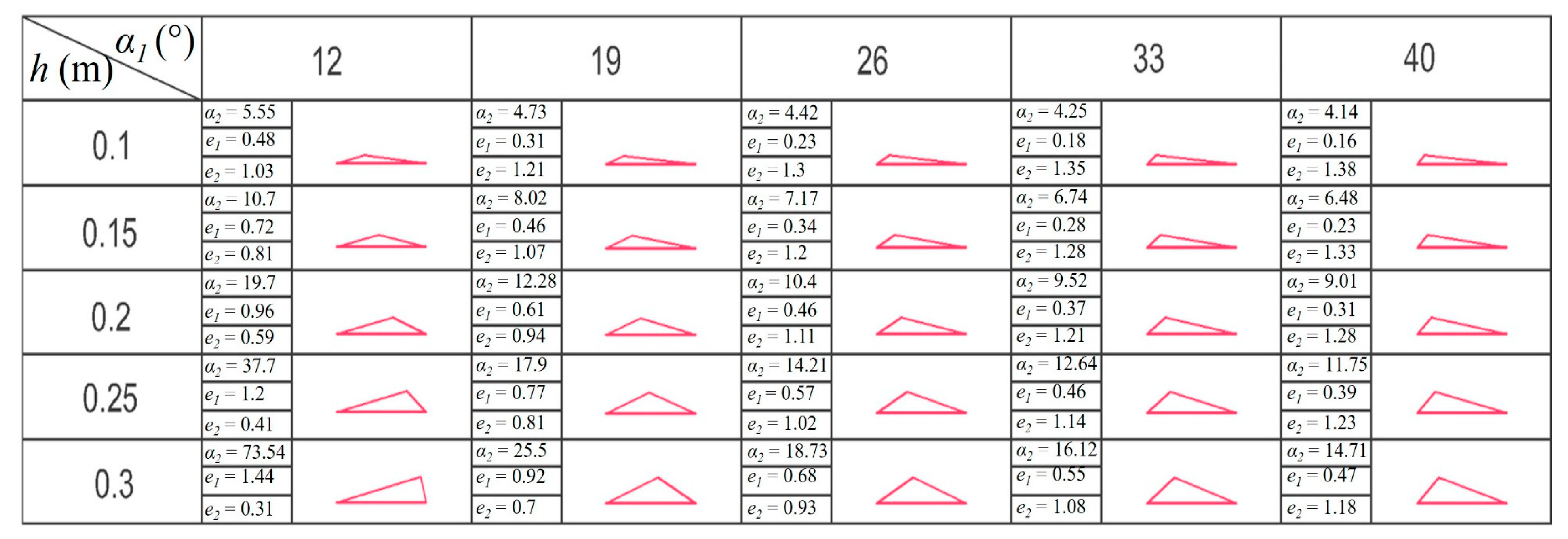
We can apply Equations (2)–(4) to identify the geometric parameters of the irregularities [27]. These equations correspond to a function of the input parameters, and the irregularity geometry can be created using these equations and the input parameters α₁, h, and l. The lengths of irregularity surfaces with and against water flow are represented by e_b and e_f, respectively (Figure 2). The irregularity angle in the flow direction and the spillway slope are known as α₂.

$${\alpha }_2={\mathit{tan}}^{-1}\left(\mathit{tan}{\alpha }_1\times \left({\displaystyle \frac{l\mathit{tan}{\alpha }_1}{l\mathit{tan}{\alpha }_1-h}}-1\right)\right)$$

(2)

$$e_f={\displaystyle \frac{h}{\mathit{sin}{\alpha }_1}}$$

(3)

$$e_b={\displaystyle \frac{h}{\mathit{sin}{\alpha }_2}}$$

(4)

2.3. Numerical Modeling

We used ANSYS-Fluent Version 2020 R2 to simplify the computation of the hydraulic parameters over the irregular surfaces of the channel bottom. ANSYS-Fluent converts scalar transport equations into algebraic equations that can be solved numerically using a controlled volume approach. For the analysis, we ran the open-channel submodel in ANSYS-Fluent, which is partially based on the volume of the fluid multiphase model. The k-ϵ turbulence model, with enhanced wall treatment conditions, served as the turbulence model to better evaluate the results at the water–rock interface [28]. For the simulations, Navier–Stokes equations were solved using averaged Reynolds numbers. In the case of stability, pressure–velocity coupling was treated using the widely used COUPLED algorithm. The results were extracted using CFD-Post, a post-processing tool that facilitates the visualization and analysis of CFD data. Table 2 presents the model input data for our 2D fluid flow modeling. We applied a 3 m·s⁻¹ velocity–inlet boundary condition; this value was defined on the basis of a sensitivity analysis. In open channels, the upstream velocity–inlet boundary conditions defined the flow velocity and relevant scalar characteristics of the flow at the flow inlet. At the outflow zone, we specified a pressure–outlet boundary condition. We assumed a no-slip boundary condition at the water–rock interface (Figure 2). The starting point for the simulation calculations was the water surface at the model’s entrance (inlet). Atmospheric pressure and a water depth of 2 m were also set in the model. We investigated grid independence to verify the accuracy of our findings. The outcomes of this evaluation are presented in Table 3, and the examination was conducted on the final irregularity, for which we also evaluated the maximum total pressure and water depth. Our grid convergence study determined that the ideal mesh size for our purposes was 10 cm.

Table 2. Input parameters used in the computational fluid dynamics (CFD) modeling.

Parameters	Value	Description
Initial flow depth	2 m	See point 3 in Figure 3
Initial flow velocity	3 m∙s−1	See point 1 in Figure 3
Inlet boundary condition	–	Velocity inlet (point 1 in Figure 2)
Outlet boundary condition	–	Pressure outlet (point 4 in Figure 2)
Unlined spillway length	50 m	–
No. of irregularities	32	–
Irregularity height (h)	10, 15, 20, 25, 30 cm
Irregularity angle (α1)	12°, 19°, 26°, 33°, 40°
Channel slope	5°	–

Table 2. Input parameters used in the computational fluid dynamics (CFD) modeling.

Parameters	Value	Description
Initial flow depth	2 m	See point 3 in Figure 3
Initial flow velocity	3 m∙s−1	See point 1 in Figure 3
Inlet boundary condition	–	Velocity inlet (point 1 in Figure 2)
Outlet boundary condition	–	Pressure outlet (point 4 in Figure 2)
Unlined spillway length	50 m	–
No. of irregularities	32	–
Irregularity height (h)	10, 15, 20, 25, 30 cm
Irregularity angle (α1)	12°, 19°, 26°, 33°, 40°
Channel slope	5°	–

Figure 3. Configurations of the various modeled spillway surface irregularities.

Figure 3. Configurations of the various modeled spillway surface irregularities.

Table 3. Grid independence study at the last irregularity.

Boundary Conditions	Structural Schemes
Maximum size of the grid cell (cm)	20	15	10	5	1
Water depth (cm)	82.1	73.3	68.9	67.9	68.1
Maximum total pressure (kPa)	52.63	60.16	63.18	63.6	63.52

Table 3. Grid independence study at the last irregularity.

Boundary Conditions	Structural Schemes
Maximum size of the grid cell (cm)	20	15	10	5	1
Water depth (cm)	82.1	73.3	68.9	67.9	68.1
Maximum total pressure (kPa)	52.63	60.16	63.18	63.6	63.52

2.4. Reduced-Scale Pilot-Plant Modeling

In the present study, the findings and accuracy of the developed equations were validated by comparing the results with those obtained from a pilot plant-scale spillway model constructed at Université du Québec à Chicoutimi, Québec, Canada. The construction details of this model have been explained in the methodology section. Figure 4 illustrates the experimental setup at Université du Québec à Chicoutimi, highlighting the instrumentation and configuration used during the study. Velocity measurements were recorded at three distinct locations along the centerline of the spillway channel—Point P₁ (at 1.5 m), Point P₂ (at 2.86 m), and Point P₃ (at 4.1 m)—with an inclination angle of 9 degrees. These measurements were performed using advanced 3D sensors, strategically positioned to ensure comprehensive data collection along the spillway length. Furthermore, to guarantee the reliability of the results, all measurements were conducted only after the flow reached steady-state conditions, eliminating potential transient effects. This meticulous approach reinforces the robustness of the validation process and underscores the alignment between the theoretical and experimental outcomes.

3. Results

We first examined the effects of surface irregularities on various hydraulic parameters, including velocity, velocity head, pressure head, and position head. To do so, we analyzed 25 irregularity 2D configurations and 4 unique 2D configurations of unlined spillway slopes. To examine the effects of irregularities on hydraulic parameters, we assessed each parameter independently. The following subsections detail our findings. We conducted separate analyses of the maximum velocity, average velocity, maximum velocity head, average velocity head, pressure head, and position head. One of our objectives was to observe the differences in energy and, subsequently, the USPD when the average and maximum velocities were considered separately. 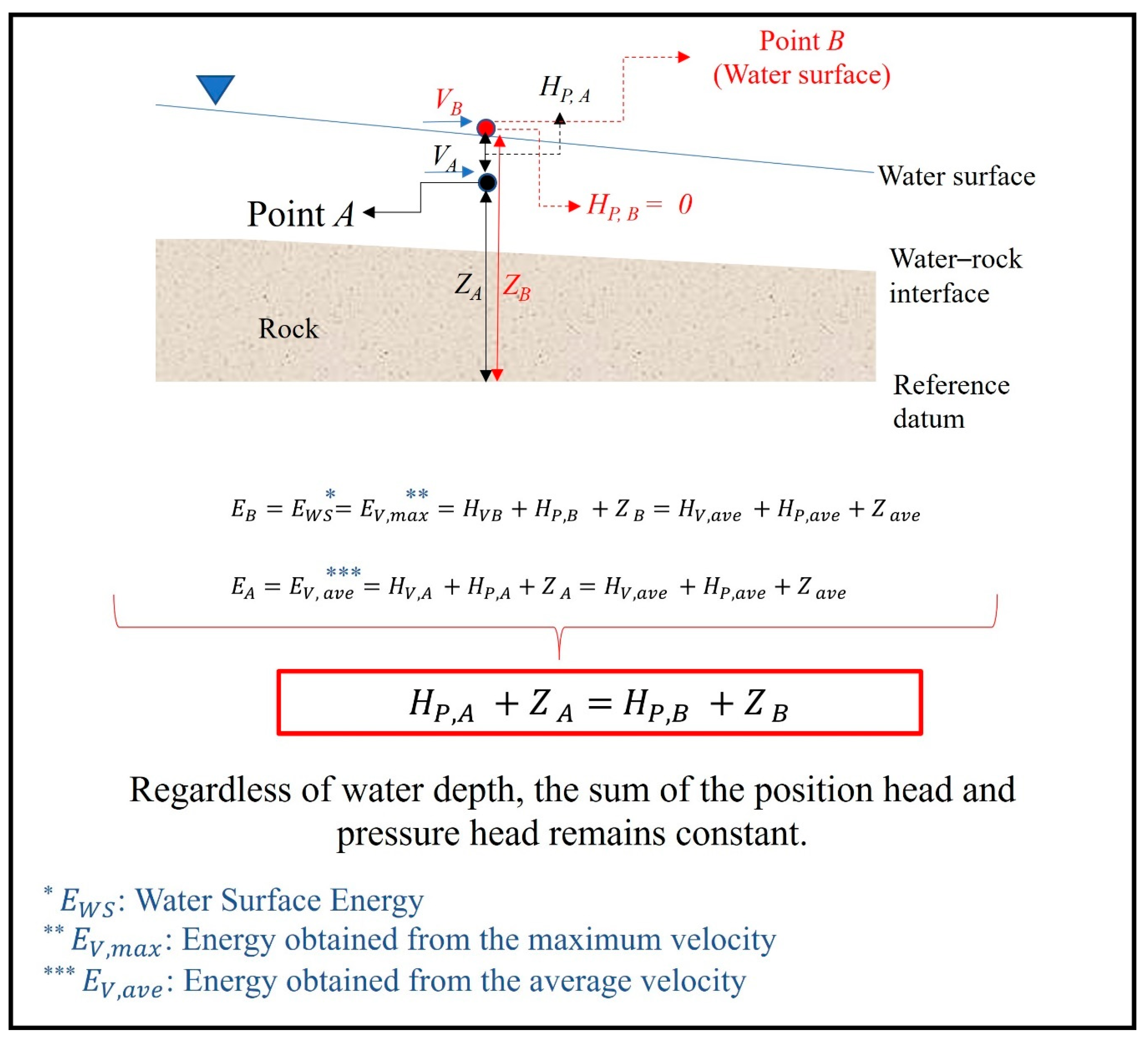From Figure 5 and Equations (5)–(7), the summation of position head and pressure head remains constant, irrespective of the variation in the location of the analysis point within the water depth. Ultimately, in examining the impact of irregularities on position head and pressure head, our analysis focused on their summation rather than analyzing each parameter individually.

In hydraulics, the hydraulic head refers to the sum of the velocity head (H_V), pressure head (H_P), and position head (Z). The relationships among (H_V), (H_P), and (Z) are described by Equations (5)–(7), respectively.

$$E=H_V+H_P+Z,$$

(5)

$$H_V={\displaystyle \frac{1}{2g}}{v}^2$$

(6)

$$H_P=d,$$

(7)

where g is the gravitational acceleration, d is the water depth, and v is the local flow velocity.

3.1. Effects of Irregularities on Maximum and Average Velocities

To estimate the maximum velocity profile, we analyzed 11 vertical cross sections along the spillway by calculating each section’s maximum velocity and water depth. Maximum velocity decreased as irregularity angle (α₁) and irregularity height (h) increased (Figure 6). The effect of height on flow velocity was greater than the effect of α₁; for instance, when α₁ was held constant (α₁ = 12), maximum velocity decreased from approximately 11.5 m∙s⁻¹ at h = 10 cm to approximately 8 m∙s⁻¹ at h = 40 cm. When height was held constant (at 10 cm), changes in α₁ did not necessarily reduce maximum velocity. For example, maximum velocity was approximately 11.5 m∙s⁻¹ for α₁ = 12 and approximately 9 m∙s⁻¹ for α₁ = 40. Interestingly, the changes in α₁ had no significant effect on the maximum velocity at higher irregularity heights (h), whereas irregularity height produced a greater impact. To estimate the average velocity along the spillway, we applied the identical approach used for our analysis of maximum velocity. To avoid redundancy and minimize the number of figures, we excluded average velocity from this section. The impact of irregularities on velocity heads aligns with the effects observed in velocity profiles, and this relationship is explored in Section 3.3, illustrating the relationship between irregularities and velocity heads.

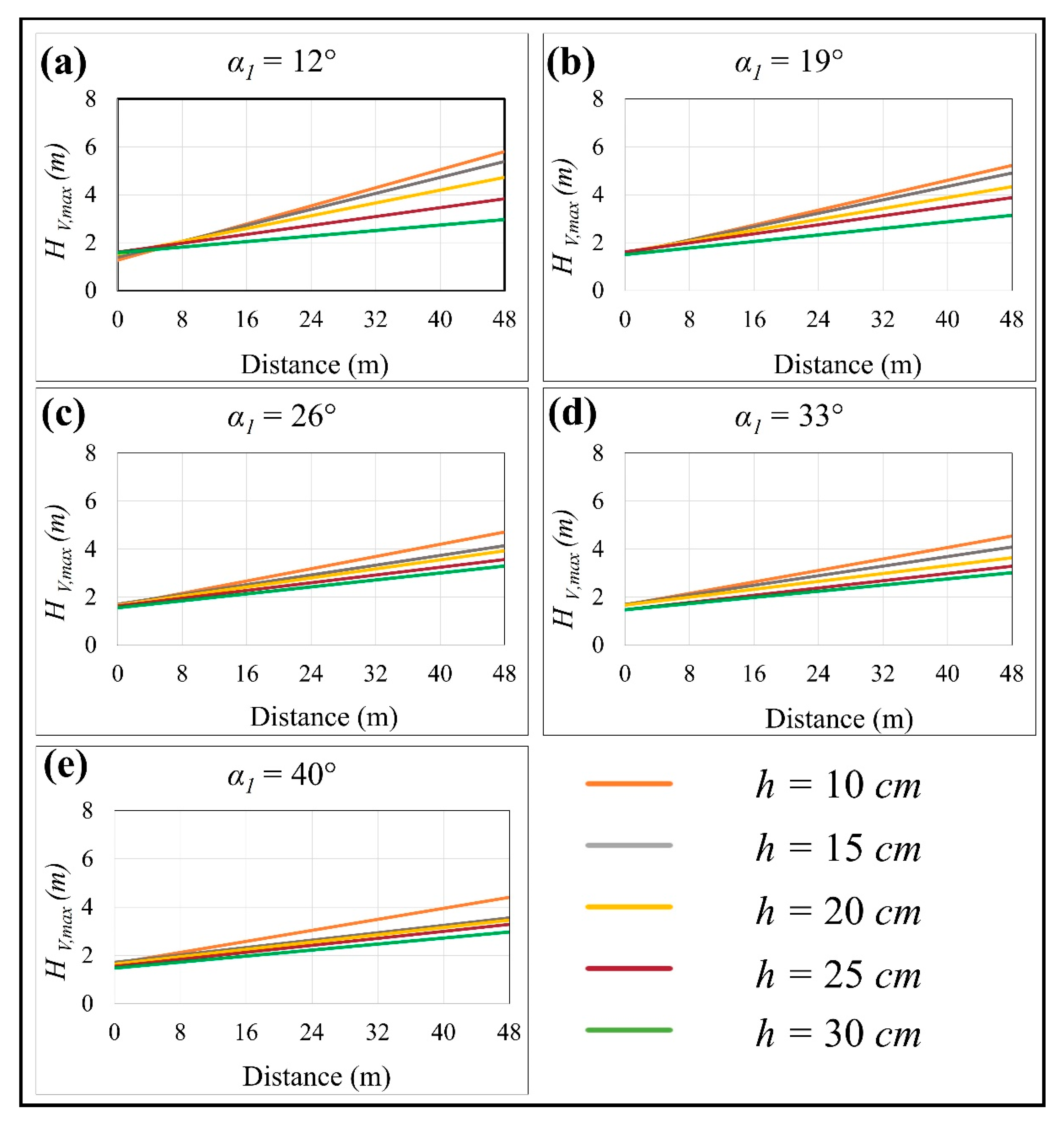
3.2. Effects of Irregularities on Maximum Velocity Head (H_V,max)

The maximum velocity head is a vital parameter in hydraulic studies. Equation (6) served to compute the maximum velocity head, and the related graphs present the numerical simulation results (Figure 7). The effects of irregularities on the maximum velocity head were similar to those illustrating their effect on maximum velocity (Figure 5).

3.3. Effects of Irregularities on Average Velocity Head (H_V,ave)

The average velocity head was determined on the basis of the average water flow velocity, and Figure 8 displays H_V,ave in nonlinear overflows. Comparing Figure 7 and Figure 8, we observe that the H_V,ave values are approximately 65% of those of H_V,max. Moreover, as α₁ increases, the impact of h on H_V,ave decreases (Figure 8).

3.4. Effects of Irregularities on Pressure Head and Position Head (H_P + Z)

We then investigated the effects of rock surface irregularities on the hydraulic parameters of the pressure head and elevation head. At a given distance x, the sum of pressure head and elevation head remained constant regardless of irregularity height (see Figure 5). Moreover, the (H_P + Z) graphs in Figure 9 overlapped, indicating an independence from rock surface irregularities and an effect of the distance parameter, which decreases upstream to downstream.

3.5. Sequential Approach for Modifying the USPD: A Stepwise Approach

3.5.1. Development of H_V,max, H_V,ave, and (H_P + Z) Equation as Functions of α₁, h, and x, Respectively

As stated earlier, we determined H_V,max using maximum velocity.

$$c_{{\alpha }_1,h}={\displaystyle \frac{H_{v,max}-H_{vi,max}}{x}}$$

(8)

where Equation (8) represents the angle coefficient of each graph in Figure 7, with a $c_{{\alpha }_1,h}$ value for each configuration.

Table 4. Angle factors of the H_V,max graphs.

	α1 = 12°	α1 = 19°	α1 = 26°	α1 = 33°	α1 = 40°
h = 0.1 m	0.0944	0.0777	0.064	0.0599	0.0571
h = 0.15 m	0.0833	0.0698	0.051	0.0499	0.0384
h = 0.2 m	0.0667	0.0569	0.0472	0.0412	0.0379
h = 0.25 m	0.0463	0.0541	0.0404	0.0379	0.0363
h = 0.3 m	0.0286	0.0473	0.0364	0.0322	0.0312

provides the corresponding $c_{{\alpha }_1,h}$ values for each configuration. H_Vi,max represents the maximum velocity at the starting point, which can be calculated using Equation (6) with the initial velocity at that point.

We used our results (Table 4) to plot the best-fit curves (and the associated equations) for $c_{{\alpha }_1,h}$ against irregularity height (h). The equations are equivalent to Equation (9).

The angle coefficients of the graphs depicted in Figure 10 are nearly equal and the graphs are almost parallel. Therefore, we calculated the average angle coefficient (a_ave) for the graphs and developed new equations for $c_{{\alpha }_1,h}$ related to the average value (a_ave). Following the substitution of the average value, we determined a corresponding set of $b_{{\alpha }_1,n}$ values (

Table 5. New y-intercepts produced on the basis of a_ave.

Tan α1	0.34432	0.48773	0.64940	0.8391
bα1	0.0918	0.0741	0.0712	0.0617
bα1,n (produced using aave = 0.1318)	0.08968	0.07412	0.0709	0.0641

).

$$y=c_{{\alpha }_1,h}={\left({\displaystyle \frac{H_{v,max}-H_{vi,max}}{x}}\right)}_{{\alpha }_1}=a_{{\alpha }_1}h+b_{{\alpha }_1}$$

(9)

Differences among the graphs in Figure 10 relate to the y-intercept ($b_{{\alpha }_1,n}$) that is altered by changing α₁. Therefore, we aimed to determine the correlation between $b_{{\alpha }_1,n}$ and Tan(α₁) using Figure 11 [Equation (10)]. After obtaining Equation (10) from the results in Figure 11, using Equation (10) and the value of a_ave (a_ave = 0.1318), we applied them in Equation (9) to derive Equation (11). Equation (11) represents H_Vi,max, and it is a function of irregularity height (h), irregularity angle (α₁), and the distance from the upstream (x). Figure 12 depicts the steps followed in developing Equation (11).

$$b_{{\alpha }_1, n}=0.0365 {\mathit{tan}{\alpha }_1}^{-0.526 }, \mathrm{and}$$

(10)

$${ H}_{v, max}=({\displaystyle \frac{0.0365}{\sqrt{\mathit{tan}{\alpha }_1}}}-0.1318h)x+H_{vi, max}.$$

(11)

We applied the same approach to derive the H_V,ave equation, which relied on the results obtained from the Ansys-Fluent software. The resulting equation, denoted by Equation (12), expresses H_V,ave as a function of α₁, h, and x. As discussed above, Equation (13) (H_P + Z) is independent of surface irregularities (α₁ and h) because the impact of irregularities on (H_P + Z) can be neglected. Referring to Figure 9, (H_P + Z) as a function of x is illustrated by Equation (13).

$$H_{v,ave}=({\displaystyle \frac{0.0234}{\sqrt{\mathit{tan}{\alpha }_1}}}-0.08h)x+H_{vi,ave}, \mathrm{and}$$

(12)

$${(H}_P+Z)=[-0.09x+{(H}_{Pi}+Z_i)]$$

(13)

3.5.2. Effects of the Spillway Slope (β) on Developed Equations for H_V,max, H_V,ave, V_max, V_ave, and (H_P + Z)

In the previous section, the equations for H_V,max, H_V,ave, and (H_V + Z) are regardless of the overall slope of the unlined spillway (β). To investigate further, we simulated additional models using spillway slopes (β) ranging from 2.5° to 15° while maintaining a smooth surface. We extracted the results of these simulations for H_V,max, H_V,ave, and (H_V + Z) and presented those of H_V,max in Figure 13. Despite the differences in β, the coefficient of the angle for each graph remained the same, as depicted in Equation (8). However, as we had already obtained the effects of irregularities on the hydraulic parameters for β = 5°, we divided the angle coefficients of the graphs in Figure 13 by the angle coefficient of the normalizer, β = 5°, as shown in Equation (14a).

Table 6. The coefficients of various normalized angles on the basis of the tangent function of the slope angle, β.

β (°)	2.5	5	10	15
tan β	0.04366	0.08749	0.17633	0.26795
Angle factor (before normalization)	0.0538	0.097	0.18	0.261
Angle factor (after normalization)	0.5546	1	1.8557	2.6907

presents the coefficients of various normalized angles using the tangent function of the slope angle, β. The corresponding diagram (Figure 14) has the horizontal axis representing tan(β) and the vertical axis representing the coefficient of the normalized angle factors obtained from the graphs in Figure 13. After obtaining the graphical equation of Figure 14, we equated it with Equation (14a), where the denominator is identical to that of Equation (11). By substituting Equation (11) and the graphical equation of Figure 14 in Equation (14a) (see points 1 and 2 in Figure 15), we obtained a new equation [Equation (14b)] for H_{V, max}, which is a function of β, α₁, h, and x.

Similarly, by applying the same technique, we could also derive new equations for (H_P + Z) and H_V,ave as a function of β [Equations (15) and (18), respectively]. Using Equations (6), (14b) and (15), we obtained equations for the maximum and average velocities [Equations (16) and (17), respectively] along the unlined spillway (Figure 15 presents how we modified the equation).

$$\mathrm{y}={\displaystyle \frac{{\left(\frac{H_{v,max}-H_{vi,max}}{x}\right)}_{\beta }}{{\left(\frac{H_{v,max}-H_{vi,max}}{x}\right)}_{\beta =5}}}$$

(14a)

$$H_{v,\mathrm{m}\mathrm{a}\mathrm{x}}=(9.51\tan \beta +0.16)({\displaystyle \frac{0.0365}{\sqrt{\tan {\alpha }_1}}}-0.1318h)x+H_{vi, max}$$

(14b)

$${ H}_{v, ave}=(7.94\tan \beta +0.34)({\displaystyle \frac{0.0234}{\sqrt{\tan {\alpha }_1}}}-0.08\mathrm{h})x+H_{vi, ave}$$

(15)

$$V_{max}=\sqrt{\left[\left(9.51\tan \beta +0.16\right)\left({\displaystyle \frac{0.0365}{\sqrt{\tan {\alpha }_1}}}-0.1318h\right)x+H_{vi, max}\right]2g}$$

(16)

$$V_{ave}=\sqrt{\left[\left(7.94\tan \beta +0.34\right)\left({\displaystyle \frac{0.0234}{\sqrt{\tan {\alpha }_1}}}-0.08h\right)x+H_{vi, ave}\right]2g}$$

(17)

$${(H}_P+Z)={(H}_{Pi}+Z_i)-\left(\mathrm{t}\mathrm{a}\mathrm{n}\beta +0.01\right)x$$

(18)

where H_Pi is the initial water depth and Z_i is the difference between levels of the analyzed section: (X₂ − X₁) · sinβ.

$$\mathsf{\Delta }\mathrm{E}={\left({ H}_{v, max}+H_P+Z\right)}_2-{\left({ H}_{v, max}+H_P+Z\right)}_1$$

(19)

$$\mathrm{U}\mathrm{S}\mathrm{P}\mathrm{D}=\rho gq{\displaystyle \frac{\mathsf{\Delta }\mathrm{E}}{\mathsf{\Delta }\mathrm{X}}}$$

(20)

We could then derive a new equation for H_V,max by considering spillway slope, irregularity height, and position along the spillway. The equation is a function of α₁, h, and x to permit a more comprehensive analysis of hydraulic parameters under various conditions. Equation (19) shows the energy loss from upstream to downstream, and Equation (20) presents our modified equation for the USPD. Notably, the abovementioned equations cannot be used with α₁ = 0° because no natural rock surfaces possess an α₁ value of absolute zero.

4. Validation, Cross-Validation, Comparison, and Practicality

In the present study, the findings and accuracy of the developed equations were validated by comparing the results with those obtained from a pilot plant-scale spillway model constructed at Université du Québec à Chicoutimi, Québec, Canada. The construction details of this model are explained in the Methodology Section.

For validation we used the maximum velocity as it was identified as the most important parameter in the equations, analyzed against the results of the experimental model. The comparison demonstrates that the equations provide results consistent with the experimental findings, as indicated by the error calculation value of 0.024, as shown in

Table 7. Comparison of the maximum velocity results as determined using our novel equation and those of the pilot plant model.

	X (Distance from Initial Point)
	P1	P2	P3
Vmax (Pilot Plant)	2.8 m/s	3.4 m/s	3.6 m/s
Vmax (Developed equation)	2.91 m/s	3.29 m/s	3.6 m/s
Error	0.038173	0.033550	0.000064
Average Error	0.023929

, by applying Equation (21). It is important to note that, for this comparison, only smooth surface conditions were evaluated to ensure the validity and consistency of the results. Figure 16 presents a comparison between the maximum velocity derived from theoretical equations (findings of this study) and that obtained from the experimental pilot plant model.

$$\mathrm{E}\mathrm{r}\mathrm{r}\mathrm{o}\mathrm{r}={\displaystyle \frac{V_{max,Developed equation}-V_{max,Pilot Plant}}{V_{max,Developed equation}}}$$

(21)

In addition, to verify the accuracy of the developed equations, we ran a cross-validation test using the data obtained from the ANSYS-Fluent simulations. We simulated another model in ANSYS-Fluent using the configuration β = 8°, α₁ = 20°, and h = 0.17 m and compared the simulation results with those of the developed equation for USPD. The cross-validation process demonstrated a consistent match between the developed equations and simulation results. Furthermore, we validated our simulations against analytical models, specifically for smooth surface configurations. Ultimately, our findings indicate that this equation is capable of predicting hydraulic parameters for unlined spillways across various irregularities.

We then compared these newly developed equations, which consider the effects of irregularities on the hydraulic parameters, with existing equations to predict the USPD of unlined spillways having irregularities. We used the equations to estimate the total energy in the upstream and downstream regions using a configuration of β = 5°, α₁ = 20°, h = 0.17 m, and L = 50 m. This configuration closely resembles the initial 50 m of unlined spillway of the Anthony dam in Australia, considering an initial velocity of 3 m·s⁻¹ [1]. The energy values obtained using the Pells equation did not incorporate the surface irregularities of the rock formation (

Table 8. Comparison of the energy results as determined using our novel equation and those of the Pells (2016) equation [1].

	Location	Maximum	Average
E modified (m)	Upstream	7.66	6.06
	Downstream	4.8	2.61
E Pells (m)	Upstream	5.05	5.05
	Downstream	2.25	2.25

). In contrast, our equation considers these irregularities, enabling the calculation of energy on the basis of either the maximum or average flow velocity. There is a clear disparity in the head loss between the upstream and downstream sections when comparing the Pells and our novel equations (Table 8). Interestingly, our method produces a slightly higher head loss. This discrepancy can be attributed to the presence of irregularities in the rock, which facilitate the transfer of energy to the rock surface, consequently leading to hydraulic erosion.

Engineers and designers can use these developed equations to predict the hydraulic parameters of unlined spillways with irregularities and optimize the design of such structures. These novel equations can help engineers better predict the hydraulic parameters (e.g., erosion and overflow) of the spillway. We also conducted simulations using heterogeneous irregularities (unlined spillway surface with various irregularity angles and heights, i.e., surfaces with irregular irregularities) to test the practicality of our equations. Despite assuming homogeneous surface irregularities, we attempted to include various irregularities in the new model; however, the energy results for heterogeneous and homogeneous models were nearly identical (Figure 17).

5. Conclusions

We developed novel equations to predict the hydraulic parameters of unlined spillways characterized by surface irregularities. Cross-validation verified the accuracy of the equations and confirmed their ability to predict the hydraulic parameters of unlined spillways with irregularities. We also demonstrated that our equations, when run compared against other existing equations in the literature, predicted the USPD of unlined spillways more accurately when considering irregularities on the rock mass surface. These novel equations account for the effects of irregularities on the hydraulic parameters, an effect neglected by other existing equations. We found that irregularities along the spillway surface affect various hydraulic parameters, and changes in irregularity height have a marked effect on hydraulic parameters. Our developed equations have been validated with experimental results obtained from a pilot plant model setup at the University of Quebec at Chicoutimi, showing an average error of 0.024. They have also been cross-validated with another numerical simulation using different configurations, which confirmed the accuracy of the developed equation. In the design of hydraulic structures, particularly unlined spillways, a pivotal aspect is delineating the erosive and resistive elements. The fundamental parameter in characterizing the erosive aspect is defining the unit stream power dissipation (USPD). It is advisable for designers to employ the developed equations in this thesis to determine the USPD, enabling a subsequent comparison with the resistive part of the phenomenon. The utilization of these equations contributes to heightened accuracy, as they take into account the geometrical parameters of the rock surface, including irregularities. Consequently, by considering a more comprehensive set of parameters, these equations enhance precision and optimize the overall design process. This study utilized two-dimensional steady-state numerical simulations to evaluate the impact of geometric surface irregularities on flow characteristics and energy dissipation in unlined spillways. While this method offered a controlled environment to investigate parametric sensitivities and refine the USPD equation, it has limitations. Specifically, 2D simulations do not capture three-dimensional turbulence structures, flow separation in transverse directions, or unsteady behaviors such as pulsations and transient surges, which can affect stream power and erosion dynamics. Additionally, the surface irregularities modeled were idealized shapes with consistent height and angle, which do not accurately represent the irregular, multiscale, and random nature of actual rock surfaces. These simplifications may influence the quantitative outcomes and generalizability of the findings. Future research should expand this analysis by using 3D transient simulations, physical experiments, and field-based surface characterizations to fully understand the hydraulic complexity and validate the enhanced USPD model under realistic conditions.

References

- Pells, S. Erosion of Rock in Spillways. Ph.D. Thesis, UNSW Sydney, Sydney, Australia, 2016. Available online: http://handle.unsw.edu.au/1959.4/56008 (accessed on 9 November 2021).
- Laursen, E.M. The total sediment load of streams. J. Hydraul. Eng. 1958, 84, 1–36. [Google Scholar] [CrossRef]
- Lacey, G. Stable channels in alluvium. Minutes Proc. Inst. Civ. Eng. 1930, 229, 259–292. [Google Scholar] [CrossRef]
- Bakhmeteff, B.A. Hydraulics of Open Channels, 1st ed.; McGraw-Hill: New York, NY, USA, 1932. [Google Scholar]
- Blench, T. Regime theory for self-formed sediment-bearing channels. Trans. Am. Soc. Civ. Eng. 1952, 117, 383–400. [Google Scholar] [CrossRef]
- Laursen, E.M.; Toch, A. Scour Around Bridge Piers and Abutments; The Iowa Highway Research Board: Iowa City, IA, USA, 1956. [Google Scholar]
- Yalin, M.S. Mechanics of Sediment Transport, 1st ed.; Pergamon Press: Oxford, UK, 1972. [Google Scholar]
- Ackers, P.; White, W.R. Sediment transport: New approach and analysis. J. Hydraul. Div. 1973, 99, 2041–2060. [Google Scholar] [CrossRef]
- Chanson, H. Hydraulic Design of Stepped Cascades, Channels, Weirs and Spillways; Pergamon Press: Oxford, UK, 1995. [Google Scholar]
- Annandale, G. Erodibility. J. Hydraul. Res. 1995, 33, 471–494. [Google Scholar] [CrossRef]
- Knighton, A.D. Fluvial Forms and Processes: A New Perspective; Arnold: London, UK, 1998. [Google Scholar]
- Darcy, H. Recherches Expérimentales Relatives au Mouvement de l’eau Dans les Tuyaux; Mallet-Bachelier: Paris, France, 1857; Volume 1. [Google Scholar]
- Weisbach, J.L. Lehrbuch der Ingenieur-und Maschinen-Mechanik: Theoretische Mechanik; Druck und Verlag von Friedrich Vieweg und Sohn: Braunschweig, Germany, 1845; Volume 1. [Google Scholar]
- Manning, R.; Griffith, J.P.; Pigot, T.F.; Vernon-Harcourt, L.F. On the flow of water in open channels and pipes. Trans. Inst. Civ. Eng. Irel. 1890, 20, 161–207. [Google Scholar]
- Cengel, Y.A.; Cimbala, J.M. Fluid Mechanics: Fundamentals and Applications, 3rd ed.; CRC Press: Boca Raton, FL, USA, 2015. [Google Scholar]
- Khodashenas, S.R.; Paquier, A. A geometrical method for computing the distribution of boundary shear stress across irregular straight open channels. J. Hydraul. Res. 1999, 37, 381–388. [Google Scholar] [CrossRef]
- Prasad, B.V.R.; Russell, M.J. Discussion of “Diffusional Mass Transfer at Sediment-Water Interface” by Nancy Steinberger and Midhat Hondzo. J. Environ. Eng. 2000, 126, 576. [Google Scholar] [CrossRef]
- Yang, S.-Q.; Lim, S.-Y. Boundary shear stress distributions in trapezoidal channels. J. Hydraul. Res. 2005, 43, 98–102. [Google Scholar] [CrossRef]
- Guo, J.; Julien, P.Y. Shear stress in smooth rectangular open-channel flows. J. Hydraul. Eng. 2005, 131, 30–37. [Google Scholar] [CrossRef]
- Seckin, G.; Seckin, N.; Yurtal, R. Boundary shear stress analysis in smooth rectangular channels. Can. J. Civ. Eng. 2006, 33, 336–342. [Google Scholar] [CrossRef]
- Severy, A.; Felder, S. Flow Properties and Shear Stress on a Flat-Sloped Spillway. In Proceedings of the 37th IAHR World Congress, Kuala Lumpur, Malaysia, 13–18 August 2017. [Google Scholar]
- Bollaert, E.; Schleiss, A. Transient Water Pressures in Joints and Formation of Rock Scour Due to High-Velocity Jet Impact; EPFL-LCH: Lausanne, Switzerland, 2002. [Google Scholar]
- Bollaert, E. The Comprehensive Scour Model: Theory and Feedback from Practice. In Proceedings of the 5th International Conference on Scour and Erosion, San Francisco, CA, USA, 7–10 November 2010. [Google Scholar]
- Kashtiban, Y.J.; Saeidi, A.; Farinas, M.-I.; Quirion, M. A Review on Existing Methods to Assess Hydraulic Erodibility Downstream of Dam Spillways. Water 2021, 13, 3205. [Google Scholar] [CrossRef]
- Kashtiban, Y.J.; Shahriar, K.; Bakhtavar, E. Assessment of blasting impacts on the discontinuities in a salt stope and pillar mine using a developed image processing. Bull. Eng. Geol. Environ. 2022, 81, 151. [Google Scholar] [CrossRef]
- Lopez, J.C.; Lopez, J.E.; Ayala, C.F.J. Drilling and Blasting of Rocks; CRC Press: Boca Raton, FL, USA, 1995. [Google Scholar]
- Kashtiban, Y.J.; Saeidi, A.; Farinas, M.-I.; Patarroyo, J. Evaluation of the Effect of Surface Irregularities on the Hydraulic Parameters within Unlined Dam Spillways. Water 2023, 15, 3004. [Google Scholar] [CrossRef]
- Kashtiban, Y.J. Development of an Equation for Evaluating Hydraulic Erosive Parameter of Unlined Dam Spillways Considering Surface Irregularities and Geometrical Parameters. Ph.D. Thesis, University of Quebec at Chicoutimi, Chicoutimi, QC, Canada, 2023. [Google Scholar]
Figure 1.
Flowchart of the modification of USPD equation taking into account irregularity geometry.
Figure 2.
Assumed spillway geometry used in our model of irregularities along an unlined rock spillway, and boundary conditions of the computational fluid dynamics (CFD) modeling.
Figure 4.
Experimental setup at Université du Québec à Chicoutimi; (a,b) Reduced-Scaled Model Schematic; (c–e) implemented experimental model for various tests at the University of Quebec at Chicoutimi.
Figure 5.
Calculation of energy at the water surface (Point B) and location of the average velocity (Point A) measurement.
Figure 6.
Maximum velocity profiles of flow along the unlined spillway; (a) α1 = 12°; (b) α1 = 19°; (c) α1 = 26°; (d) α1 = 33°; (e) α1 = 40°.
Figure 7.
Maximum velocity head profiles of flow along the unlined spillway; (a) α1 = 12°; (b) α1 = 19°; (c) α1 = 26°; (d) α1 = 33°; (e) α1 = 40°.
Figure 8.
Average velocity head profiles of the flow along the unlined spillway; (a) α1 = 12°; (b) α1 = 19°; (c) α1 = 26°; (d) α1 = 33°; (e) α1 = 40°.
Figure 9.
Profiles of (HP + Z) along the unlined spillway; (a) α1 = 12°; (b) α1 = 19°; (c) α1 = 26°; (d) α1 = 33°; (e) α1 = 40°.
Figure 10.
Relationship between and irregularity height (h).
Figure 11.
Correlation between tan(α1) and the new y-intercepts of the angle factor graphs.
Figure 12.
Methodology for modifying the USPD on the basis of irregularity height and angle (α1 and h).
Figure 13.
Simulation results for HV,max as a function of distance.
Figure 14.
Relationship between the coefficient of the normalized angle factors of HV,max and the unlined spillway slope (β).
Figure 15.
Methodology to modify the USPD for application on an unlined spillway slope (β).
Figure 16.
Comparison of Vmax from the pilot plant model and developed equations.
Figure 17.
Comparison of model outputs run using heterogeneous and homogeneous irregularities.