Stormwater Pollution of Non-Urban Areas—A Review

Abstract

Stormwater runoff from areas with specific industrial, agricultural or logistic land use comprises a significant source of water pollution, yet research on its specific composition remains limited compared to urban stormwater pollution. This review synthesizes findings from different studies to analyze sampling methods, types of pollution parameters and their associated concentration ranges across various non-urban land use types, including industrial and commercial zones, transportation infrastructure (ports, airports, highways, railways) and agricultural areas. Studies differed in sample strategy, investigated phase (water, sediment) and analyzed chemical parameters. The latter can be grouped into sum parameters (e.g., total suspended solids (TSS), chemical oxygen demand (COD)), metals (e.g., nickel, copper, zinc, lead), nutrients (e.g., nitrogen, phosphorus), organic micropollutants (e.g., polycyclic aromatic hydrocarbons (PAH), perfluoroalkyl acids (PFAA)) and microbial contaminants. Results indicate that pollutant loads vary widely depending on land use, with industrial and railway areas showing the highest metal contamination, while agricultural and livestock farming areas exhibit elevated nutrient and microbial concentrations. The heterogeneity of the sampling, analysis and subsequent data processing hindered the statistical condensation of data from different studies. The findings underscore the need for standardized monitoring methods and tailored stormwater treatment strategies to mitigate pollution impact effectively.

1. Introduction

Stormwater runoff as a non-point source pollution is the primary contributor to the pollution of receiving waters [1]. Only 38% of the European Union’s water bodies meet environmental quality standards for good chemical status [2]. Pinpointing pollution sources is important to effectively manage surface water pollution.

While pollutant dynamics in urban areas are well studied, research on industrially utilized areas remains limited, as shown in Figure 1. The number of search results for the keywords “stormwater” and “urban” in Scopus was eleven times higher than the number of search results for the combination of “stormwater” and “industry”. Hits for other land use classes were even lower in number.

Given the specific industrial, agricultural or logistic activities and the diversity of functional areas (e.g., production, storage, transport, washing), highly specific loads are to be expected. Chow et al. [3] emphasized that stormwater pollution is strongly influenced by major anthropogenic activities in an area, underscoring the need for local stormwater monitoring programs, namely, for specific operational conditions.

Since urban stormwater pollution has been (and will continue to be) well investigated, this review explicitly focuses on non-urban areas. These include industrial or commercial areas, transportation areas such as ports, airports, highways and railways, as well as agricultural areas. This study aims to provide an overview of existing studies in this apparently poorly investigated field and to determine the specific types of stormwater pollution associated with different land uses. To achieve this, a range of studies were evaluated to answer the following questions:

• Which substances are relevant in different sectors?
• What are the concentration ranges of these substances?
• Which sampling methods are commonly employed for measurement?
• Can specific factors affecting pollution be identified?

2. Materials and Methods

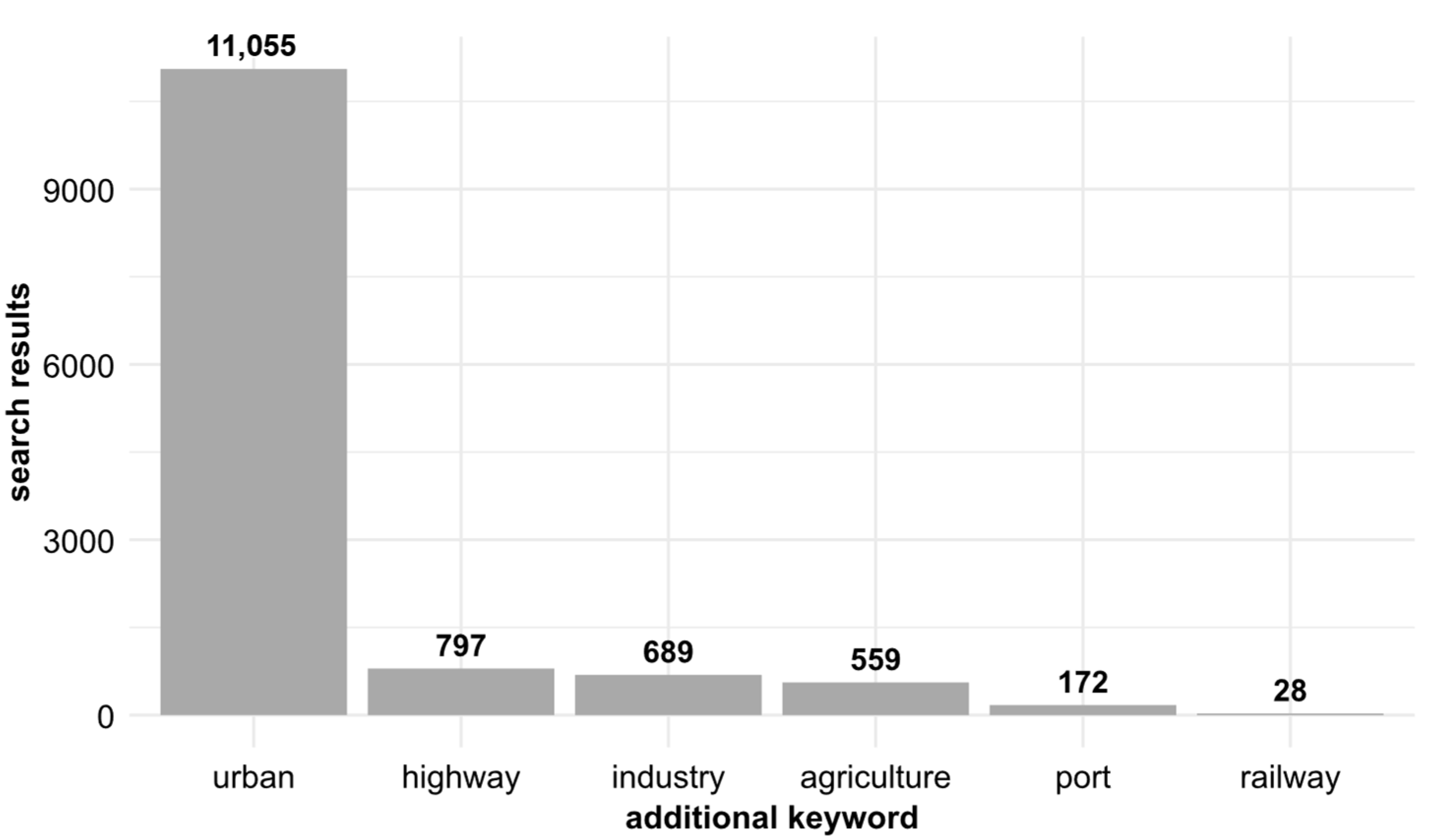
2.1. Literature Search and First Evaluation

The literature search was primarily conducted using scientific literature databases. The main search was conducted in Scopus (https://www.scopus.com/) and Absclust (https://absclust.com/) (using the Semantic Scholar database) from June to November 2024. It was initially performed using the keywords ‘stormwater’ or ‘stormwater pollution’ combined with different land use designations. The designations used were “industry”, “agriculture”, “port”, “airport”, “railway”, “commercial” and “waste disposal”.

Upon an initial review of the search results, many studies were excluded as they did not fall within the scope of this review paper. A total of 91 studies were shortlisted, by skimming the abstracts of the search results, with attention given to whether a study included pollutant measurements for specific land use areas.

These 91 studies were subsequently evaluated to determine their final relevance to this review. The primary evaluation criterion was the availability of measured values of pollution parameters. Only 28 studies met this criterion by providing quantitative pollutant measurements presented in tabular form.

The reasons for excluding studies from this review were varied, but certain common patterns emerged. Some studies investigated pollution in natural water bodies but did not specify the sources of the pollutants in sufficient detail. Consequently, it was impossible to attribute pollutant loads to particular land use types. The most frequent exclusion criterion was the absence of measured data, even when a study topic aligned with the focus of this review.

Six studies that included pollutant measurements presented their data in graphs or box plots rather than distinct numeric values in tables. The computer vision assisted software WebPlotDigitizer 5.2 was used to extract the numerical data from the plots.

2.2. Working with the Values

Given the substantial variability among the monitoring programs in the reviewed studies, this review aimed to categorize the reported values as systematically as possible based on sampling methods, land use types and monitored pollution parameters. These values were then analyzed, clustered and discussed.

In many cases, the raw measurement data from the conducted monitoring programs were not published individually but reported as aggregated statistical values, such as mean or median and standard deviation. The following list provides an overview of the types of values reported by each study:

• Individual values: [4,5,6,7,8,9,10,11,12,13]
• Statistical mean values: [1,3,14,15,16,17,18,19,20,21,22,23,24,25,26,27,28]
• Statistical median values: [28,29,30,31,32]
• Statistical minimum and maximum: [33,34]
• 25th and 75th percentile: [28]

For certain nutrients, such as nitrates, some studies reported values specifically for nitrates, while others measured nitrate nitrogen. This means that for the same molar concentration of the compound, different mass concentrations were observed. Similar inconsistencies were observed for nitrites, ammonium, ammonia and phosphate. In such cases, the reported values were converted to ammonium nitrogen, nitrite nitrogen, nitrate nitrogen and phosphate phosphorus to ensure consistent concentration data in the dataset. Depending on the analytical method, total ammonia concentration was either measured in the ionic form NH₄⁺ or as undissociated ammoniac gas NH₃. If only toxic NH₃ were of interest, its share would need to be calculated for given pH and temperature. However, none of the studies provided this information. Accordingly, it was assumed that the provided ammonia or ammonium concentrations always reflected the sum of both forms and were standardized as ammonium nitrogen.

One study [3] reported concentrations of soluble reactive phosphorus (SRP), which was assumed to correspond to PO₄³⁻-P [35].

For fecal coliforms and Escherichia coli, only a single source was identified for each. Consequently, these parameters were analyzed separately.

Mathematical analyses and visualization were conducted using RStudio 2024.09.1+394 software.

3. Results

3.1. The Compiled Data

Appendix A compiles in separate tables all found data for one land-use type (see Section 3.4). The tables were subdivided according to two criteria: (i) the measured phase and (ii) the parameter group. Some studies directly investigated runoff (fluid phase), while others performed particle analysis (solid phase), as further described in Section 3.3. The grouping of parameters is explained in Section 3.5. If data existed for different functional areas for certain land use types, these subgroups were listed in separate columns.

When multiple studies provided measurements for similar land uses, these values were not combined, since even for the same land use type, specific operational activities can differ significantly. Furthermore, monitoring approaches were often not comparable (see Section 3.3). For each reported measurement, the lowest and highest values from the respective studies are provided, along with the number of observations.

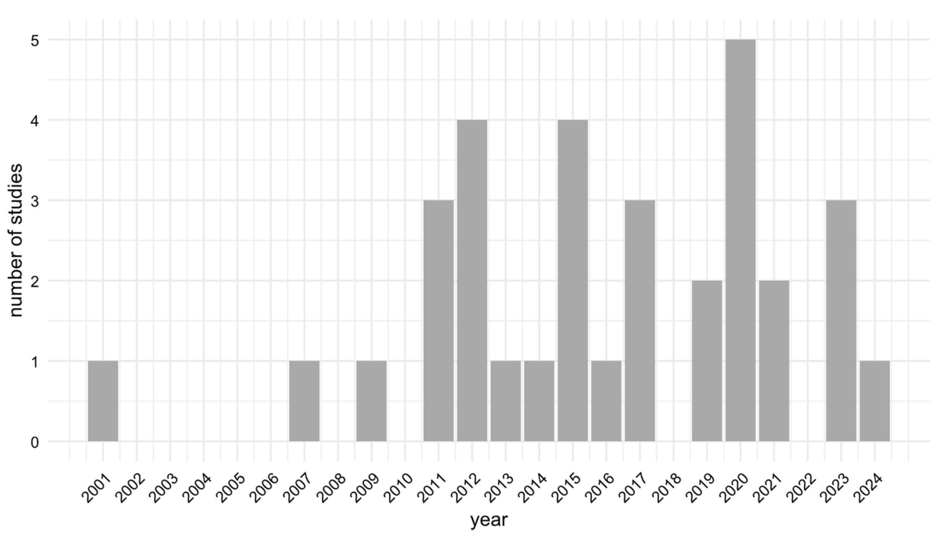
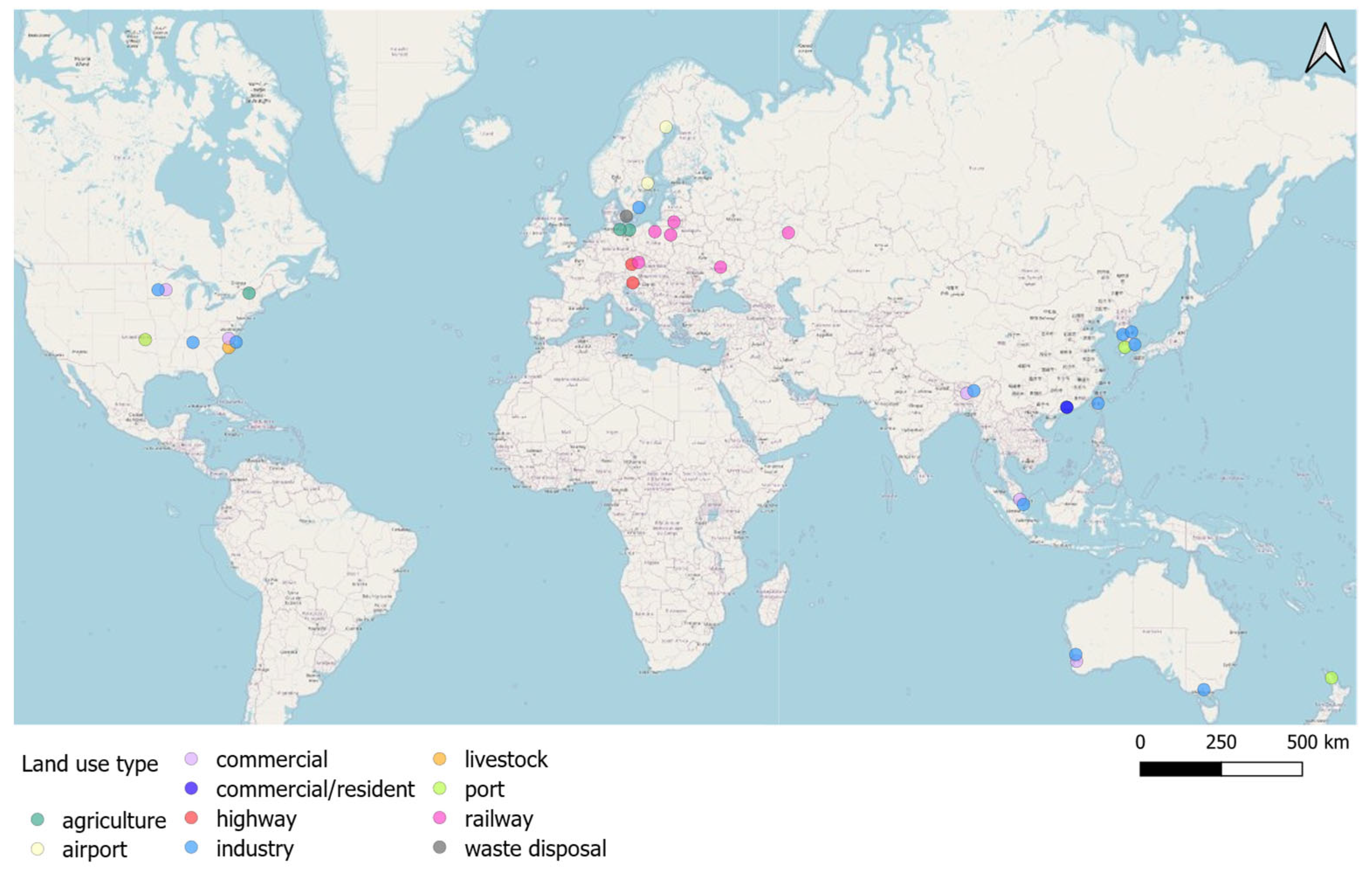
3.2. Geographical and Temporal Distribution

The temporal frequency distribution shows the publishing years of the reviewed studies (Figure 2). According to the search criteria, only three studies had addressed stormwater quality in non-urban areas until 2010. Since then, the number of publications has increased, but remains low, with a maximum of five studies in 2020.

Figure 3 shows the geographical distribution of the monitoring sites of the reviewed studies. No evaluable monitoring data was found for South America or Africa. Of the 14 monitoring sites spread across various European countries, 10 were located in Eastern Europe. Notably, railway areas were primarily sampled in Eastern European countries. The United States of America had the highest number of monitoring sites (eight) and exhibited a high diversity of monitored land uses. A total of ten monitoring sites were established in Asia, with four of these sites located in South Korea. The majority of these were located within industrial areas. Australian studies provided data from four monitoring sites. Monitoring of commercial areas usually appeared together with the monitoring of industrial areas.

3.3. Sampling Methods

The reviewed studies employed a variety of sampling methods, as illustrated in Figure 4. However, a distinction can be made between two main sampling approaches:

• Sampling of the liquid phase
• Sampling of the solid phase

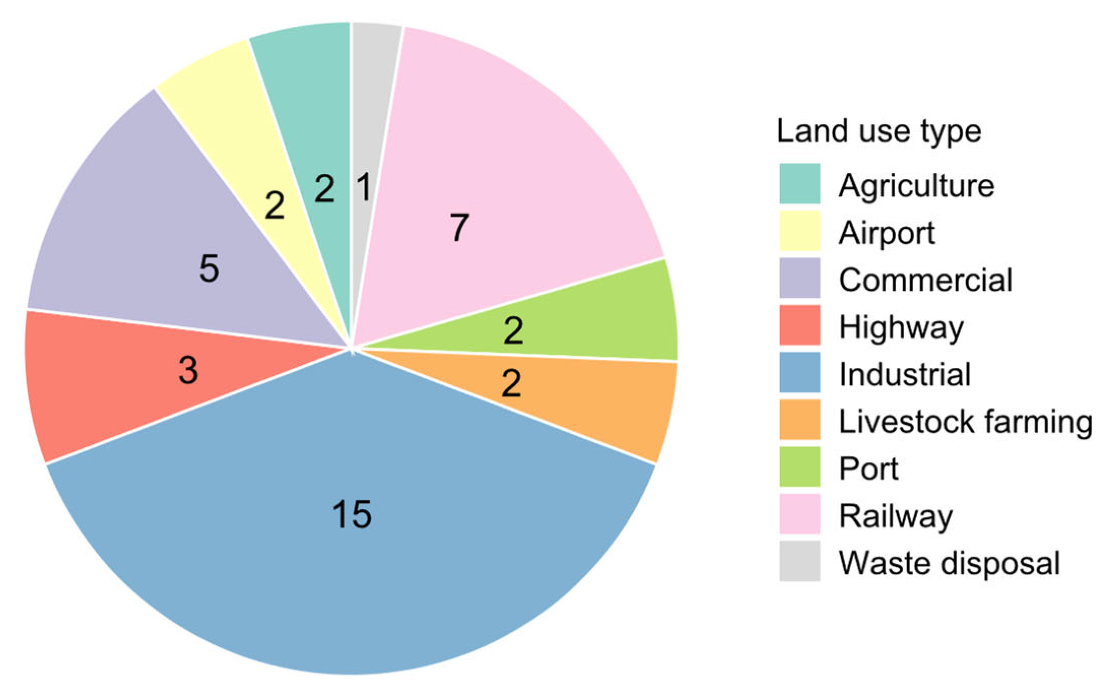
Various specific techniques were employed within these primary sampling categories. In some cases, samples were collected directly from streams or drainage ditches, primarily in agricultural or livestock farming areas.

Stormwater runoff was typically sampled using either single grab samples or composite samples, which were collected at predefined time or flow intervals during a rain event. In some cases, stormwater discharges were also sampled from collection basins or retention ponds.

Solid phase sampling was also carried out using various techniques. Generally, it can be distinguished between soil sampling or the collection of sediments, taken from either the environment or surfaces. These surface sediments were either swept dry or vacuumed wet or dry. Studies focusing on railway areas predominantly employed soil sampling, while one study specifically investigated railway ballast stones used in track beds. The sampling of road-deposited sediments was most commonly conducted as part of industrial site assessments.

3.4. Land Uses

For the various industrial land uses, urban areas were deliberately excluded from the analysis.

The proportion of studies examining each land use category is presented in Figure 5. The majority of studies focused on industrial areas, as this represented the most common yet least specific land use category. Railway and highway areas were the next most frequently monitored, followed by commercial areas. For the remaining land uses, only one or two relevant sources were identified.

As the term “industry” covers a wide range of activities, the specific areas monitored varied considerably, resulting in significant differences in the measured values. Heavily utilized industrial sites, for instance, are expected to exhibit higher pollutant loads compared to areas designated for light industrial activities. To avoid generalizing these differences, an attempt was made to specify the land uses as precisely as possible. However, as the studies defined the land uses with varying degrees of precision, it was decided to retain the general classifications as umbrella terms. The following land use subcategories were established:

• Industry: not specified; light industry; equipment storage; smelting (various); mixed
• Commercial: commercial; mixed with residential
• Railway: bridge/siding/railroad; platform/station; stabling yard/loading; cleaning
• Port: port surfaces; port basin
• Waste disposal: storage; composting; car park; road
• Agriculture: drainage ditch; intensively grazed pastures; outfalls draining mixed agricultural areas; biogas plants
• Livestock farming: main concentrated animal feeding operations (CAFO) drainage; secondary CAFO drainage; yard areas

Many studies varied in the level of detail provided when describing their monitoring areas. Some studies did not specify the exact function of an industrial area, necessitating the inclusion of a “not specified” category. The specificity of the remaining subcategories was constrained by the level of detail available in the respective studies. Due to the limited descriptions of the “highway” and “airport” land uses, further subdivision of these categories was not feasible.

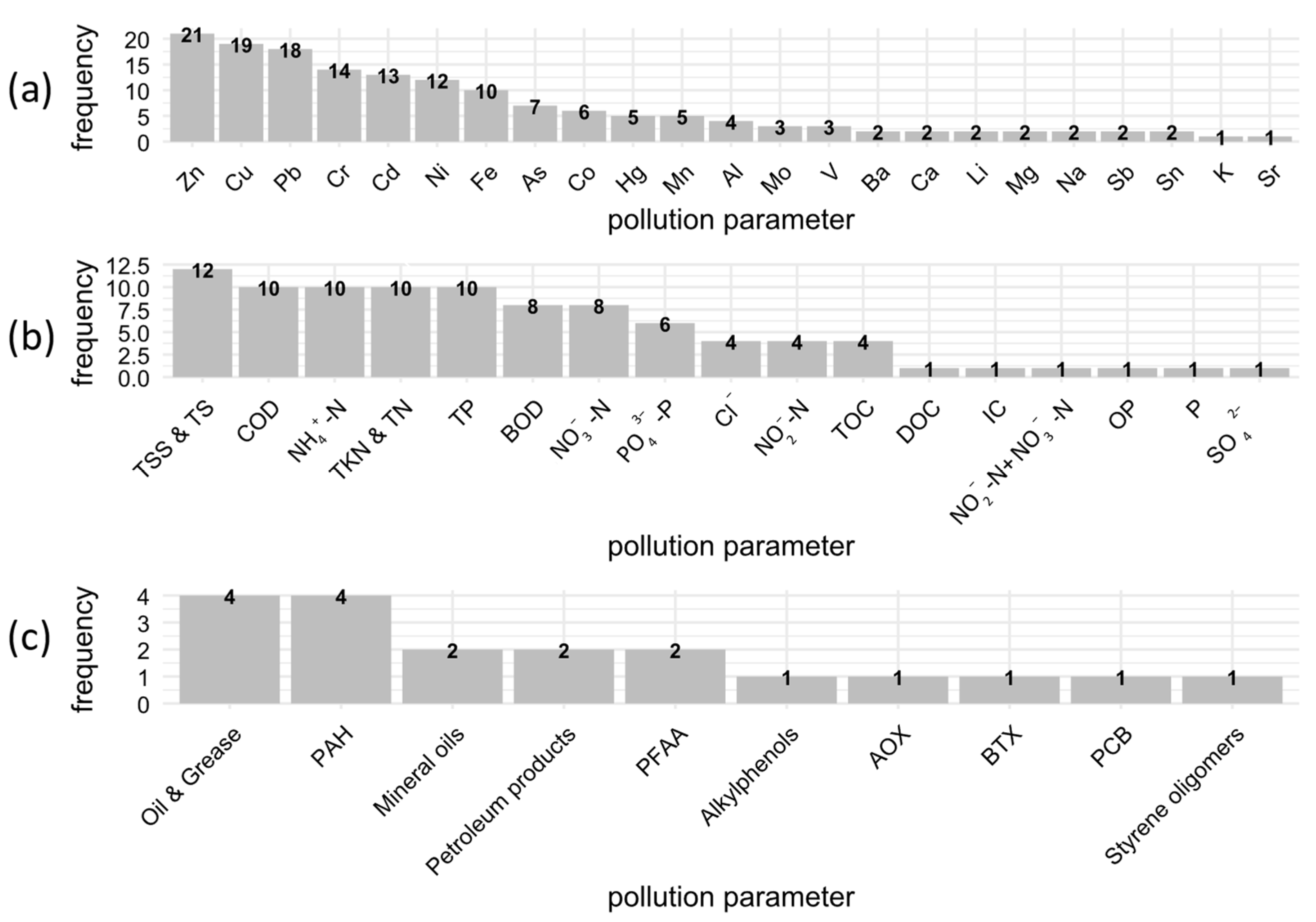
3.5. Pollution Parameters

3.5.1. Parameter Groups

The diverse range of applications within the industrial sector was associated with very specific pollutant loads, resulting in a large set of pollutants.

All parameters measured in the considered studies were incorporated into the analysis. All parameters were categorized into three groups (Figure 6):

• Group I—metals
• Group II—solids, biodegradable organic matter, nutrients and macro-pollutants
• Group III—organic (micro-)pollutants

For comparison, six groups of parameters were established for urban areas: solids, heavy metals, biodegradable organic matter, organic micropollutants, pathogenic microorganisms and nutrients [36]. All of these were identified in this review.

The number of studies reporting measurements for each parameter is provided in Figure 6. The parameter abbreviations are explained in the Abbreviations section at the end of this review. Metals such as nickel, copper, zinc, lead or chromium were the most frequently detected. The prevalence of the monitoring of metals in this sector is likely attributable to the pervasive consideration of metal processing companies as a dominant category within the industrial land use type. For solids, biodegradable organic matter, nutrients and macropollutants (group II), most studies examining non-urban areas focused on total suspended solids (TSS), chemical oxygen demand (COD) and total phosphorus (TP). A substantial number of studies also examined different forms of nitrogen compounds, such as ammonium or nitrate. Organic micro-pollutants were the least frequently monitored in non-urban areas, despite their high relevance in urban areas [37]. This is partly explicable by the investigated land-use types and its potential pollution inventory. In addition, awareness of and analytical capabilities for some emerging contaminants (namely PFOS) have improved in recent years.

Distinct patterns in monitoring programmes were revealed by analysing the selection of parameters across different land uses.The widest range of monitored metals was observed in the industry, railway and airport sectors, followed by port, highway and waste disposal areas. In commercial areas, only two metals were analyzed. Studies dealing with agricultural and livestock farming areas did not monitor any metals. Group II was monitored across most land uses with a relatively high number of respective parameters, except in railway and port areas. However, the highest number of parameters related to Group II was analyzed in industrial and commercial areas, followed by other land uses. At least one organic micro-pollutant was monitored for every land use except for port, agriculture and livestock farming areas. However, comparability across land uses was limited, as many parameters were analyzed for only one specific land use.

3.5.2. Coliform Bacteria

As previously mentioned, only two studies that aligned with the objectives of this review measured coliform bacteria. Mallin et al. [16] monitored fecal coliform concentrations in natural streams draining concentrated animal feeding operations (CAFO), while Kominami et al. [23] measured E. coli concentrations from a dairy farm area. Both studies collected their samples from streams or drainage ditches.

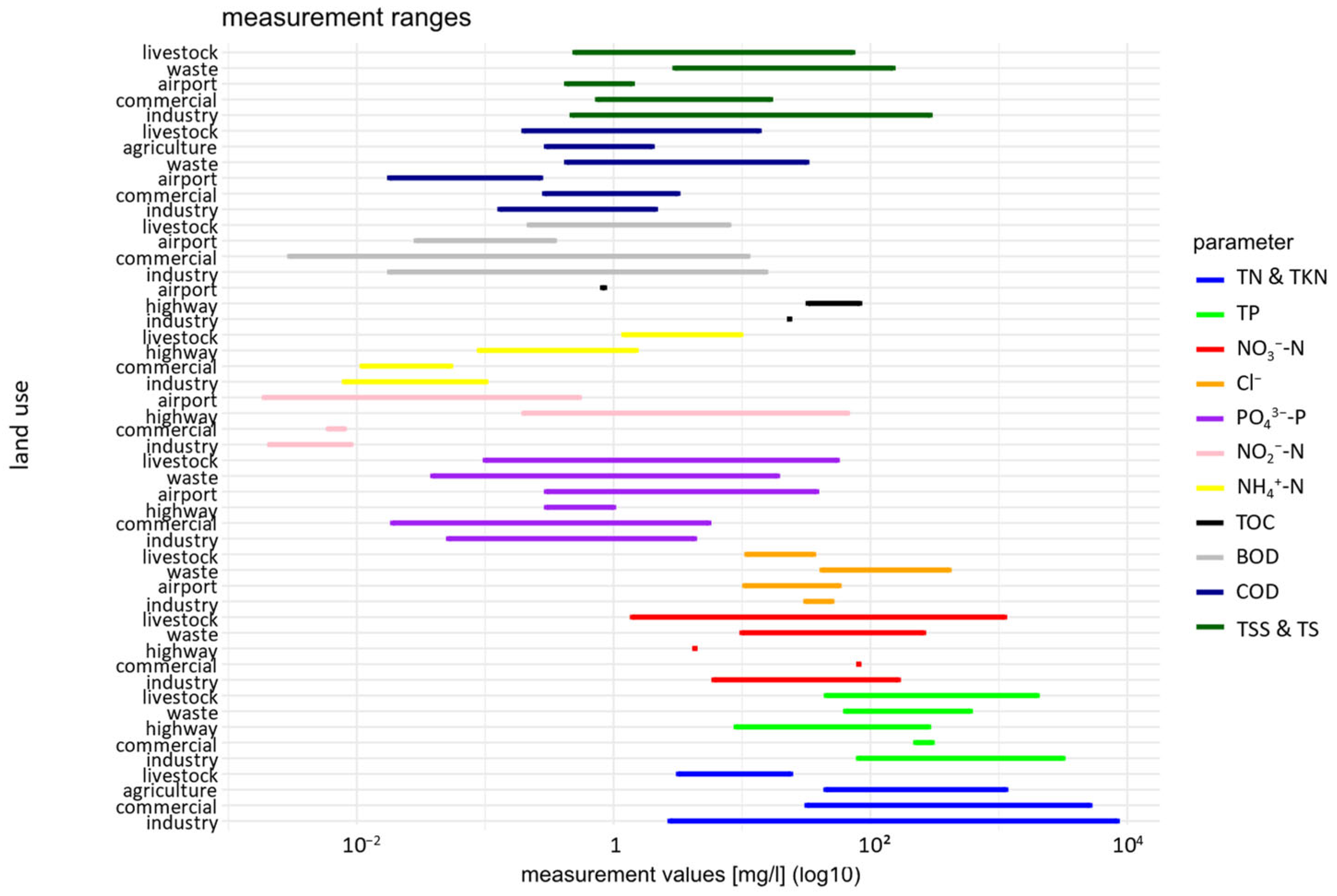
3.6. Measurement Ranges

The availability of data was sparse, for several reasons. The sampling methods, monitored land use types and pollution parameters varies greatly, making direct comparisons between measurements difficult. However, the following diagrams aim to summaries the collected results, including only parameters that were monitored across at least three different land uses. The bars represent the minimum and maximum values for each parameter and land use, as listed in the tables in Appendix A.

Figure 7 represents the metal concentrations in samples of the fluid phase. For nickel, lead, chromium and aluminum, the highest maximum concentrations were observed for the industry sector, keeping in mind that several studies were performed in metal working companies. For iron, lead, cadmium and zinc, highway areas had comparably high maximum concentrations. Port areas generally showed lower Pb, Zn and Cu concentrations than other land use types. Waste disposal sites showed the highest concentrations for copper. Airport areas had relatively high copper and zinc concentrations.

Figure 8 presents the concentrations for solids, biodegradable organic matter, nutrients and macropollutants measured in the fluid phase. The difference between the sampling of stormwater runoff and receiving waters complicated the comparability, as pollutant concentrations become diluted in receiving waters. Despite broad concentration ranges, industrial and commercial areas showed high maximum NO₃⁻-N concentrations. TSS concentrations were in similar ranges for agricultural, commercial and industrial areas. Pollution levels in highway runoff generally appeared high and showed maximum concentrations for Cl⁻ and NO₃⁻-N. Waste disposal areas exhibited high concentrations of TN, TP, NH₄⁺-N, TOC, BOD and COD. Livestock areas showed high maximum concentrations of nutrients like NO₃⁻-N, PO₄³⁻-P and NH₄⁺-N. Similarly, water samples from agricultural areas were characterized by elevated nutrient concentrations.

Figure 9 illustrates metal concentrations measured in the solid phase. Unlike Figure 7, this one includes only three land use types—port, railway and industry. This is because sampling in the solid phase was only conducted in these cases. The maximum concentrations of mercury, arsenic, lead, zinc and copper were significantly higher in industrial areas than in port or railway areas. Railway areas, especially railway sidings and platform areas, exhibited high metal concentrations [7]. Figure 9 suggests that port areas exhibited lower metal concentrations than industrial and railway areas.

4. Discussion

4.1. Origin of the Loads

The industrial land use type generally displayed high metal concentrations. Salehi et al. [30] stated that high concentrations of inorganic pollutants can, for example, originate from contaminant release by the storage of utility-related equipment and fill materials. High concentrations of mercury, arsenic, lead, zinc and copper from industrial areas primarily originated from industrial areas associated with the smelting industry and resulted from spillage and diffusion during transportation [15]. Additionally, metal processing industries induced high metal pollution [14]. Since most studies in the industrial sector were undertaken in or around metalworking companies, the results were partly biased. Different patterns would be expected in other industrial sectors, e.g., the food processing industry. High TSS concentrations in industrial areas can stem from various sources, e.g., rock and soil fragments, dirt, debris, decaying plant and animal matter or industrial waste [21]. Accordingly, TSS alone, i.e., without information about its origin or chemical composition, provides only limited information as a pollutant parameter.

Despite broad concentration ranges, industrial and commercial areas showed high maximum NO₃⁻-N concentrations. Elevated NO₃⁻-N concentrations in industrial areas may result from industrial emissions, nitrogen containing raw materials and industrial processes [21]. In commercial areas, NO₃⁻-N mainly originated from restaurants and food stalls [22] or the decay of vegetable and fruit residues [21].

For iron, lead, cadmium and zinc, highway areas had comparably high concentrations in stormwater. Comparative values for urban road runoff [38] fell within the lower range of these measurements, indicating that highway concentrations sometimes significantly exceeded those of urban roads. While in Figure 8, pollution levels in highway runoff appear high, Gotvajn et al. [4] argued otherwise. In this case, the maximum concentrations represented an extreme case rather than a typical range, as peak concentrations occurred after a heavy rain event following a prolonged dry period [4].

High metal concentrations in the railway sector resulted from abrasion processes of brakes, rails, wheels and power lines, as they are characterized by the materials of these components [33]. For instance, composite brakes significantly reduce metal emissions compared to cast-iron or sintered iron brakes [39]. Railway areas, especially railway sidings and platform areas, exhibited high metal concentrations [7]. Samarska et al. [9] examined railway ballasts from track beds and identified two primary sources of the high metal concentrations. Metals such as nickel, chromium or copper are components of railway steel and enter the environment through the abrasion of rails and wheels [9]. Furthermore, Samarska et al. [9] found that railway ballasts themselves can be considered a moderate source of metals.

Port areas generally showed lower Pb, Zn and Cu concentrations than other land use types. However, Kane-Sanderson et al. [24] attributed relatively high Al concentrations to a coal stockpile, linking them specifically to that monitoring site. Jeong et al. [5] was the only study that examined metals in the solid phase from port areas by sampling road-deposited sediments (RDS) and port sediments. Analysis of RDS indicated that the highest metal concentrations correlated with proximity to various industrial activities, such as metal production sites, parking lots or tire repair shops [5]. Elevated concentrations of zinc and copper in port sediments originated from boat antifouling paints, making them the primary source of metal pollution in these sediments [5]. These findings suggest that shipping traffic directly contributes to the pollution of port sediments, whereas RDS pollution in port areas primarily originates from other sources, such as industrial activities. In ports, the pollution potential is highly dependent on the stored/handled materials and the specific management. For example, runoff from modern container terminals with widely automated carrier systems can be supposed to be only slightly polluted, in contrast to bulk goods terminals. Accordingly, further studies should clearly describe their investigation methods for the various functional zones in ports.

Metal concentrations in waste disposal sites varies greatly, depending on the characteristics and amounts of the waste handled, making generalizations difficult [29]. Therefore, waste management areas should be assessed individually. Waste disposal areas exhibited high concentrations of TN, TP, NH₄⁺-N, TOC, BOD or COD, which again depended on the specific waste volume and composition [29].

Although airport areas showed the lowest metal concentrations, one study reported relatively high copper and zinc concentrations [10], highlighting the need for further attention in monitoring programs. Nitrogen concentrations in airport areas mainly result from de-icing processes and therefore vary seasonally [10].

The highest ammonium concentrations from livestock farming areas were recorded near spray fields, indicating a direct link. The main sources for high nitrate concentrations are swine CAFO waste, poultry litter and cattle manure, all deposited on land [16]. Similarly, agricultural areas experience elevated nutrient concentrations due to fertilizer use, necessitating close monitoring of solids, biodegradable organic matter, nutrients and macropollutants. A specific pollution source for stormwater in livestock farms and on biogas plants is the handling of feeding biomass in open silos. This requires both a strict hydraulic separation of different functional zones and consequent sweeping [32].

4.2. PAH and PFAA

For organic (micro-)pollutants, comparability is difficult, because most were only considered in one or two different monitoring programs. Polycyclic aromatic hydrocarbons (PAH) and perfluoroalkyl acids (PFAA) were almost the only organic pollution parameters that were considered in three or more monitoring programs, which is why they are discussed separately here.

The transportation sector, particularly railway areas, is linked to high PAH concentrations [7], ranging from 2.3 to 59.508 mg/kg [7,19]. PAH contamination in railway areas was therefore significantly higher than in industrial areas, where concentrations ranged from 0.236 to 2.42 mg/kg. However, the potential for direct comparisons between these two land types is limited, as railway samples were taken from soil, whereas industrial area samples were taken from lake tributaries.

PAH contamination in railway areas originate mainly from substances used for rolling stock operations, such as machine grease, fuel oils and transformers oils [7]. Hong et al. [17] reported that industrial areas have significantly higher concentrations of persistent toxic substances (PTS), including PAHs, compared to urban and rural areas. In that study, the identified PAHs primarily originated from petroleum products and byproducts of petroleum and coal combustion [17]. PAH pollution on highways mainly results from vehicle exhaust emissions [40].

PAHs pose significant risks, as their associated metabolites are often carcinogenic, mutagenic and teratogenic [41], with adverse or toxic effects on aquatic organisms [17].

PFAAs are highly persistent, toxic and ubiquitously present in the environment [11]. Their production for various applications has led to high PFAA concentrations in specific land use types [11]. One of these applications is aqueous firefighting foam [11], commonly used in airport areas [10]. Perfluorooctane sulfonic acid (PFOS), a PFAA compound, was found in stormwater runoff in airport areas at concentrations between 0.058 and 0.23 μg/L [10].

PFOS concentrations in stormwater runoff near industrial areas were significantly higher than those in residential or commercial runoff, primarily due to being washed off certain industrial products by rain [11]. Industrial applications of PFOS include semiconductor or electronics companies, as well as the apparel, medical device and pharmaceutical equipment industries [42].

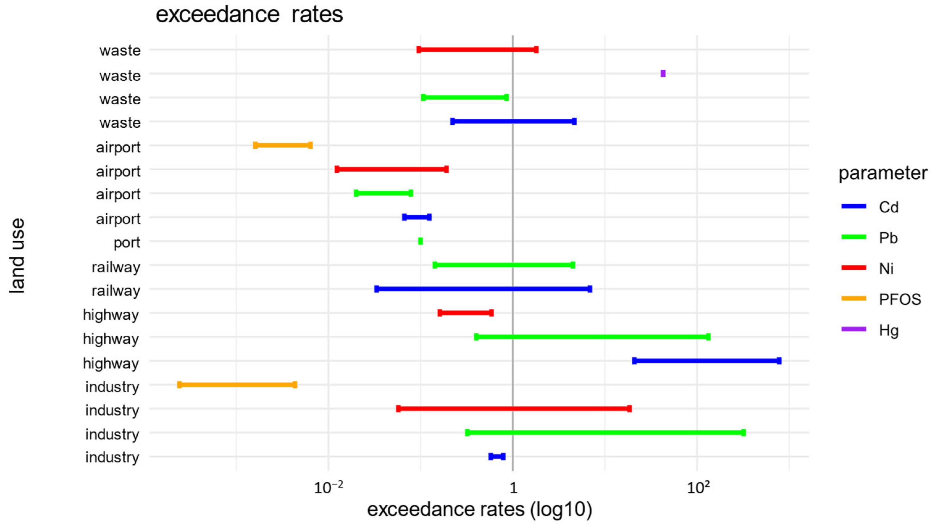
4.3. Comparison with Environmental Quality Standards

4.3.1. Threshold Values of the European Commission’s Water Framework Directive (WFD)

Neither national nor international legislations for water pollution explicitly define discharge concentrations for stormwater pollution. The most relevant reference values are those established for ambient water quality in surface waters. Regulations for surface waters vary by country. The data analyzed in this review originate from sampling sites distributed across multiple countries. To contextualize the measurements and assess potential risks, this review utilized the environmental quality standards (EQS) defined by the European Commission’s Water Framework Directive (WFD). The WFD defines priority substances for surface waters and establishes EQS for them, specified in annual average (AA) and maximum allowable concentrations (MAC).

Substances, that are defined as priority by the WFD and appear in this review are cadmium, lead, mercury, nickel and PAHs and PFOS [43].

Table 1. Environmental quality standards (EQS) for priority substances in mg/L according to the Water Framework Directive (WFD) [43].

Priority Substance	AA-EQS 1	MAC-EQS 2
Cd 3	≤0.00008	≤0.00045
Pb	0.0012	0.014
Hg	-	0.00007
Ni	0.004	0.034
PAH	1.7 × 10−7	0.00027
PFOS	6.5 × 10−7	0.036

Notes: ¹ AA: annual average. ² MAC: maximum allowable concentration. ³ values for water hardness class 1.

compiles the corresponding EQS values.

Table 2. Frequency of exceedances of environmental quality standards (EQS) of the Water Framework Directive (WFD) for measurement values from Appendix A.

Land Use Type	Substance	Number of Values (n)	Exceedance of AA (n)	Exceedance of MAC (n)
Industry	Cd	2	2	0
	Pb	9	9	7
	Ni	3	1	1
	PFOS	2	2	0
Highway	Cd	2	2	2
	Pb	2	2	1
	Ni	2	1	1
Railway	Cd	3	2	2
	Pb	5	5	3
Port	Pb	1	1	0
Airport	Cd	3	0	0
	Pb	3	0	0
	Ni	3	2	0
	PFOS	2	2	0
Waste	Cd	7	7	2
	Pb	7	7	0
	Hg	1	-	1
	Ni	7	6	1

shows the frequency of exceedance of EQS from Table 1 for the measurement values distributed in Appendix A. Airport areas exhibited the lowest number of exceedances. Although the exceedances of AA-EQS values for industry and waste disposal areas appear high, only some maximum values exceeded the MAC-EQS values as well. For highway and railway areas, the number of exceedances was relatively high for both EQS.

For stormwater discharges, comparing event-specific discharge concentrations with AA-EQS is not meaningful, and instead, MAC-EQS should be applied. For the more specific identification of relevant land-use types and parameters, an exceedance rate, calculated by dividing the minimum and maximum values set out in Appendix A by the MAC-EQS, is presented in Figure 10 This rate can also be interpreted as the required dilution factor in the receiving water to fall below the MAC-EQS. In the majority of cases, the maximum values exceeded the limit values while the minimum values often fell below the limits. Nevertheless, the range of exceedance of values for mercury in waste disposal areas (exceedance ratio = 43) and for cadmium in highway areas (exceedance ratio = 21–780) were alarming high. The found PFOS concentrations from airport and industry areas did not reach the MAC-EQS, but it is worth mentioning that they invariably surpassed the AA-EQS. Consequently, it was not possible to exclude the likelihood of the significant contamination of stormwater by PFOS.

PAH concentrations in highway areas fell below the detection limit of 0.00006 mg/L [4]. Apart from the study by Gotvajn et al. [4], no other sources were found that measured PAH concentrations in the liquid phase. The detection limit of 0.00006 mg/L exceeds the AA threshold for PAHs, making it unclear whether actual concentrations surpassed or fell below the benchmark. Ravindra et al. [44] investigated the sources, emission factors and regulation of PAHs and identified industries and highways as significant sources of PAH emissions. Therefore, it is imperative that potential sources of pollution are identified through targeted monitoring.

Because PAHs and PFAAs pose a significant environmental hazard, and for PFAAs, detected concentrations partially exceeded benchmark levels, more studies should take these substances into consideration when assessing the pollution of industrially utilized areas.

4.3.2. Coliform Bacteria

The geometric mean concentrations of fecal coliforms reported by Mallin et al. ranged from 220 CFU/100 mL to 9126 CFU/100 mL across seven sampling sites. The lowest concentrations were observed at the sites farthest from livestock farming areas. The highest fecal coliform concentrations were detected at sampling sites closest to spray fields. However, all geometric mean concentrations exceeded the referred threshold values set by the State of North Carolina for fecal impairment of water bodies [16].

The geometric mean concentrations for E. coli reported by Kominami et al. ranged from 3000 to 441,000 mpn/100 mL across eleven sampling sites. The highest concentrations were recorded in a ditch immediately downstream of a dairy farm. The measured concentrations in two bathing lakes within the study area exceeded Vermont’s threshold value of 77 E. coli/100 mL for beach bathing waters, with a mean concentration of 3000 mpn/100 mL [23].

These findings suggest that agricultural areas, especially those associated with livestock farming, contribute significant coliform bacteria loads. It is important to note that the monitoring programs relied on grab sampling in streams, which limited the ability to determine the specific pollutant loads from agricultural areas or the exact concentrations in runoff from these areas.

4.4. Stormwater Treatment

The exceedance of EQS values for multiple pollutants across various non-urban land uses indicated that stormwater requires treatment before being discharged into surface waters. The individual treatment technology is dependent on the pollution pattern and main transportation pathway. Since many pollutants are predominantly transported particle-bound (like most metals), effective particle removal is often highly efficient. Dissolved and degradable pollutants (COD, BOD, ammonia) require biological treatment. For pure sedimentation systems, the efficiency for small particles is limited [45]. Bioretention systems and constructed wetland systems combine particle removal and biodegradation and provide some adsorption capacity, making them widely applied technologies for stormwater pollutant removal [46]. Bioretention systems have been proven to be effective for removing metals and organic micropollutants [47]. Constructed wetlands achieve good removal of particulate matter due to sedimentation and filtration processes [46]. Additionally, both systems can achieve the effective degradation of organic matter, nitrification and some retention of phosphorous [48,49]. They are also known to reduce hygienic parameters [50]. However, the treatment efficiency for specific pollutants depends on the technical design of the stormwater treatment system and has to be individually adapted to specific pollution types. Specific organic micro-pollutants would only be retained by advanced treatment (activated carbon, ozonation). However, designing and operating these systems for stormwater treatment is technically and economically challenging. Consequent infrastructural and operational separation of most pollutant areas in combination with consequent sweeping can minimize treatment efforts.

4.5. Differences in Sampling Methods and Presentation of Results

As discussed above, the different sampling methods made a reliable comparison of pollution levels difficult. The pollutant concentrations in stormwater runoff had significant temporal and spatial variations [22]. To gather representative values, monitoring has to be carried out accordingly. Often discussed is the first flush with highest concentration in the beginning of a rain event, but deviating dynamics can also be observed, depending on the characteristics of the catchment and the individual rain event. The high concentration ranges in Figure 7, Figure 8 and Figure 9 partly resulted from different sampling and monitoring approaches across the evaluated studies. In particular, measurements from studies that used grab sampling had limited representativeness due to the concentration dynamics during one event. [1]. Against this background, it is questionable that the United States Environmental Protection Agency (US EPA) guidelines for stormwater monitoring advocate the utilization of grab sampling [51].

When comparing the two composite sampling methods, flow-proportional sampling provides less bias than time-proportional sampling [52] and would provide the most representative results for a whole rain event. One severe disadvantage of this sampling method is significantly higher expenditure and costs [1]. Namely, reliable flow metering can become difficult in specific conditions. As alternative, the sampler could be controlled by a rain gage, assuming a proportionality between rain intensity and runoff as performed in [32]

In any case, standardized approaches are needed, because the differences in monitoring methods lead to difficulties when interpreting and comparing the measured values. It seems to be questionable to apply sophisticated statistical methods or modelling approaches on scarce datasets, i.e., which do not completely fulfil standards of sampling size [1]. In order to create better representativeness and comparability between different monitoring programs, monitoring techniques should be harmonized.

The high variance in sampling methods is problematic, as are the varied approaches to the presentation of results. As shown in Section 2.2, the reviewed studies had high variances in how they provided their measurement values. Individual values are only comparable to a limited extent with, for example, mean values. The presence of these discrepancies compromises the feasibility of conducting a representational statistical analysis. If condensed statistical data are provided, it would be helpful to provide the initial raw data set.

4.6. Surface Loads

Surface loads are usually specified in milligrams per area or as site mean concentrations [3], but with one exception, none of the considered papers provided this unit for their pollutants. The respective measurement values are distributed in

Table A19. Agriculture [g/(m²*d)].

Pollution Parameter	Biogas Plant
COD	3.78–41.70 [32] n = 9
TP	0.0005–0.08 [32] n = 9
TN	0.02–0.33 [32] n = 9

. Investigations on nutrient contaminants and COD were carried out for biogas plant areas, for which Cramer et al. [32] determined high loads.

Another parameter used to characterize stormwater pollution is the pollutant annual mass load per unit of area given as kg/ha×a [36], which would require systematic long term monitoring. This parameter would, in turn, also make it possible to derive annual discharge loads and mean annual concentrations, e.g., to compare with AA-EQS.

5. Conclusions

This review points out the role of non-urban impervious areas in contributing to stormwater pollution, with pollutant concentrations frequently exceeding environmental quality standards. The analysis revealed that industrial and transportation-related areas exhibited high levels of heavy metals, while agricultural and livestock areas contributed substantial nutrient and microbial loads. Additionally, the presence of organic micropollutants, such as PAHs and PFAAs, raises concerns about long-term environmental and human health risks.

A key challenge identified was the inconsistency in sampling methodologies, which complicated data comparability and trend analyses across different land uses. Standardized monitoring programs and improved sampling techniques are recommended to enhance data reliability. Moreover, given the exceedance of regulatory thresholds for multiple pollutants, stormwater treatment technologies should be adapted to site-specific pollutant profiles.

When performing this study, it became obvious that the pollution of areas with specific industrial, agricultural or logistic land-use has a relevance that contradicts the underrepresentation across monitoring programs. While this review indicates a general dependence of pollutant loads on the investigated land use types, existing data remain insufficient to fully capture these connections. A significantly larger dataset with more extensive and standardized measurements is needed to validate these trends and identify influencing factors more precisely. A further investigation should be conducted to assess whether the incorporation of grey literature, like institutional publications or university graduate and undergraduate theses, has the potential to enhance the current data situation. The information provided in this review can potentially guide policy development by identifying land-use-specific pollutant risks and monitoring needs. By enhancing systematic monitoring and deriving best management practices, the environmental impact of stormwater pollution from non-urban areas could be significantly reduced.

References

1. Lee, H.; Swamikannu, X.; Radulescu, D.; Kim, S.; Stenstrom, M.K. Design of stormwater monitoring programs. Water Res. 2007, 41, 4186–4196. [Google Scholar] [CrossRef]
2. Nickel, J.P.; Sacher, F.; Fuchs, S. Up-to-date monitoring data of wastewater and stormwater quality in Germany. Water Res. 2021, 202, 117452. [Google Scholar] [CrossRef]
3. Chow, M.F.; Yusop, Z.; Shirazi, S.M. Storm runoff quality and pollutant loading from commercial, residential, and industrial catchments in the tropic. Environ. Monit. Assess. 2013, 185, 8321–8331. [Google Scholar] [CrossRef]
4. Gotvajn, A.Ž.; Zagorc-Končan, J. Bioremediation of highway stormwater runoff. Desalination 2009, 794–802. [Google Scholar] [CrossRef]
5. Jeong, H.; Choi, J.Y.; Lim, J.; Shim, W.J.; Kim, Y.O.; Ra, K. Characterization of the contribution of road deposited sediments to the contamination of the close marine environment with trace metals: Case of the port city of Busan (South Korea). Mar. Pollut. Bull. 2020, 161, 111717. [Google Scholar] [CrossRef]
6. Chong, N.-M.; Chen, Y.-C.; Hsieh, C.-N. Assessment of the quality of stormwater from an industrial park in central Taiwan. Environ. Monit. Assess. 2012, 184, 1801–1811. [Google Scholar] [CrossRef]
7. Wiłkomirski, B.; Sudnik-Wójcikowska, B.; Galera, H.; Wierzbicka, M.; Malawska, M. Railway transportation as a serious source of organic and inorganic pollution. Water Air Soil Pollut. 2011, 218, 333–345. [Google Scholar] [CrossRef] [PubMed]
8. Strelkov, A.K.; Stepanov, S.V.; Teplykh, S.Y.; Sargsyan, A.M. Monitoring Pollution Level in Railroad Right-of-Way. Procedia Environ. Sci. 2016, 32, 147–154. [Google Scholar] [CrossRef]
9. Samarska, A.; Kovrov, O.; Zelenko, Y. Investigation of Heavy Metal Sources on Railways: Ballast Layer and Herbicides. J. Ecol. Eng. 2020, 21, 32–46. [Google Scholar] [CrossRef]
10. Jia, Y.; Ehlert, L.; Wahlskog, C.; Lundberg, A.; Maurice, C. Water quality of stormwater generated from an airport in a cold climate, function of an infiltration pond, and sampling strategy with limited resources. Environ. Monit. Assess. 2017, 190, 4. [Google Scholar] [CrossRef]
11. Xiao, F.; Simcik, M.F.; Gulliver, J.S. Perfluoroalkyl acids in urban stormwater runoff: Influence of land use. Water Res. 2012, 46, 6601–6608. [Google Scholar] [CrossRef] [PubMed]
12. Šeda, M.; Šíma, J.; Volavka, T.; Vondruška, J. Contamination of soils with Cu, Na and Hg due to the highway and railway transport. Eurasian J. Soil Sci. (EJSS) 2017, 6, 59–64. [Google Scholar] [CrossRef]
13. Kamali, M.; Alamdari, N.; Esfandarani, M.S.; Esfandarani, M.S. Effects of rainfall characteristics on runoff quality parameters within an industrial sector in Tennessee, USA. J. Contam. Hydrol. 2023, 256, 104179. [Google Scholar] [CrossRef] [PubMed]
14. Jeong, H.; Choi, J.Y.; Lee, J.; Lim, J.; Ra, K. Heavy metal pollution by road-deposited sediments and its contribution to total suspended solids in rainfall runoff from intensive industrial areas. Environ. Pollut. 2020, 265, 115028. [Google Scholar] [CrossRef]
15. Jeong, H.; Choi, J.Y.; Ra, K. Potentially toxic elements pollution in road deposited sediments around the active smelting industry of Korea. Sci. Rep. 2021, 11, 7238. [Google Scholar] [CrossRef]
16. Mallin, M.A.; McIver, M.R.; Robuck, A.R.; Dickens, A.K. Industrial Swine and Poultry Production Causes Chronic Nutrient and Fecal Microbial Stream Pollution. Water Air Soil Pollut. 2015, 226, 407. [Google Scholar] [CrossRef]
17. Hong, S.; Lee, Y.; Yoon, S.J.; Lee, J.; Kang, S.; Won, E.-J.; Hur, J.; Khim, J.S.; Shin, K.-H. Carbon and nitrogen stable isotope signatures linked to anthropogenic toxic substances pollution in a highly industrialized area of South Korea. Mar. Pollut. Bull. 2019, 144, 152–159. [Google Scholar] [CrossRef]
18. Forsström, T. Miljörapport 2023, 1st ed.; SYSAV: Malmö, Sweden, 2024. [Google Scholar]
19. Wierzbicka, M.; Bemowska-Kałabun, O.; Gworek, B. Multidimensional evaluation of soil pollution from railway tracks. Ecotoxicology 2015, 24, 805–822. [Google Scholar] [CrossRef]
20. Sarukkalige, R.; Priddle, S. Assessment of Urban Stormwater Quality in Western Australia. In Proceedings of the 2nd International Conference on Environmental Engineering and Applications, Shanghai, China, 19–21 August 2011. [Google Scholar]
21. Khatun, A.; Bhattacharyya, K.G.; Sarma, H.P. Variability of pollutant build-up parameters in different land uses of Guwahati City, Assam, India. Int. J. Sci. Res. Publ. 2014, 10, 1–7. [Google Scholar]
22. Li, D.; Wan, J.; Ma, Y.; Wang, Y.; Huang, M.; Chen, Y. Stormwater runoff pollutant loading distributions and their correlation with rainfall and catchment characteristics in a rapidly industrialized city. PLoS ONE 2015, 10, e0118776. [Google Scholar] [CrossRef]
23. Kominami, H.; Lovell, S.T. An adaptive management approach to improve water quality at a model dairy farm in Vermont, USA. Ecol. Eng. 2012, 40, 131–143. [Google Scholar] [CrossRef]
24. Kane-Sanderson, P.L.; Poynter, M.R. Northport Stormwater: A shellfish friend or foe? In Australasian Coasts & Ports 2017: Working with Nature; Engineers Australia, PIANC Australia and Institute of Professional Engineers New Zealand: Barton, ACT, Australia, 2017. [Google Scholar]
25. Kayhanian, M.; Fruchtman, B.D.; Gulliver, J.S.; Montanaro, C.; Ranieri, E.; Wuertz, S. Review of highway runoff characteristics: Comparative analysis and universal implications. Water Res. 2012, 46, 6609–6624. [Google Scholar] [CrossRef]
26. Kaczala, F.; Salomon, P.S.; Marques, M.; Granéli, E.; Hogland, W. Effects from log-yard stormwater runoff on the microalgae Scenedesmus subspicatus: Intra-storm magnitude and variability. J. Hazard. Mater. 2011, 185, 732–739. [Google Scholar] [CrossRef] [PubMed]
27. Vaiškūnaitė, R.; Jasiūnienė, V. The Analysis of Heavy Metal Pollutants Emitted by Railway Transport. Transport 2020, 35, 213–223. [Google Scholar] [CrossRef]
28. Nayeb Yazdi, M.; Sample, D.J.; Scott, D.; Wang, X.; Ketabchy, M. The effects of land use characteristics on urban stormwater quality and watershed pollutant loads. Sci. Total Environ. 2021, 773, 145358. [Google Scholar] [CrossRef]
29. Marques, M.; Hogland, W. Stormwater run-off and pollutant transport related to the activities carried out in a modern waste management park. Waste Manag. Res. 2001, 19, 20–34. [Google Scholar] [CrossRef]
30. Salehi, M.; Aghilinasrollahabadi, K.; Salehi Esfandarani, M. An Investigation of Stormwater Quality Variation within an Industry Sector Using the Self-Reported Data Collected under the Stormwater Monitoring Program. Water 2020, 12, 3185. [Google Scholar] [CrossRef]
31. Tränckner, J.; Koch, M. Leitfaden zur Sachgerechten Niederschlagswasserbewirtschaftung auf Landwirtschaftsbetrieben und Biogasanlagen; Rostock: Thousand Oaks, CA, USA, 2023. [Google Scholar]
32. Cramer, M.; Rinas, M.; Kotzbauer, U.; Tränckner, J. Surface contamination of impervious areas on biogas plants and conclusions for an improved stormwater management. J. Clean. Prod. 2019, 217, 1–11. [Google Scholar] [CrossRef]
33. Vo, P.T.; Ngo, H.H.; Guo, W.; Zhou, J.L.; Listowski, A.; Du, B.; Wei, Q.; Bui, X.T. Stormwater quality management in rail transportation--past, present and future. Sci. Total Environ. 2015, 353–363. [Google Scholar] [CrossRef]
34. Yang, F.; Gato-Trinidad, S.; Hossain, I. (Eds.) Evaluating the Water Quality of Stormwater Runoffs in Urban Area. In Proceedings of the 18th International Conference on Environmental Science and Technology (CEST2023), Athens, Greece, 28 August–2 September 2023. [Google Scholar]
35. Dodds, W.K. Misuse of inorganic N and soluble reactive P concentrations to indicate nutrient status of surface waters. J. North Am. Benthol. Soc. 2003, 22, 171–181. [Google Scholar] [CrossRef]
36. Barbosa, A.E.; Fernandes, J.N.; David, L.M. Key issues for sustainable urban stormwater management. Water Res. 2012, 46, 6787–6798. [Google Scholar] [CrossRef] [PubMed]
37. Zhang, K.; Zheng, Z.; Mutzner, L.; Shi, B.; McCarthy, D.; Le-Clech, P.; Khan, S.; Fletcher, T.D.; Hancock, M.; Deletic, A. Review of trace organic chemicals in urban stormwater: Concentrations, distributions, risks, and drivers. Water Res. 2024, 258, 121782. [Google Scholar] [CrossRef] [PubMed]
38. Li, W.; Shen, Z.; Tian, T.; Liu, R.; Qiu, J. Temporal variation of heavy metal pollution in urban stormwater runoff. Front. Environ. Sci. Eng. 2012, 6, 692–700. [Google Scholar] [CrossRef]
39. Gustafsson, M.; Blomqvist, G.; Håkansson, K.; Lindeberg, J.; Nilsson-Påledal, S. Järnvägens föroreningar—Källor, Spridning och Åtgärder: En Litteraturstudie; Statens väg-och Transportforskningsinstitut: Linköping, Sweden, 2007. [Google Scholar]
40. Crépineau, C.; Rychen, G.; Feidt, C.; Le Roux, Y.; Lichtfouse, E.; Laurent, F. Contamination of pastures by polycyclic aromatic hydrocarbons (PAHs) in the vicinity of a highway. J. Agric. Food Chem. 2003, 51, 4841–4845. [Google Scholar] [CrossRef]
41. Heintzman, L.J.; Anderson, T.A.; Carr, D.L.; McIntyre, N.E. Local and landscape influences on PAH contamination in urban stormwater. Landsc. Urban Plan. 2015, 142, 29–37. [Google Scholar] [CrossRef]
42. Glüge, J.; Scheringer, M.; Cousins, I.T.; DeWitt, J.C.; Goldenman, G.; Herzke, D.; Lohmann, R.; Ng, C.A.; Trier, X.; Wang, Z. An overview of the uses of per- and polyfluoroalkyl substances (PFAS). Environ. Sci. Process. Impacts 2020, 22, 2345–2373. [Google Scholar] [CrossRef]
43. Publications Office of the European Union. Directive 2013/39/EU of the European Parliament and of the Council; Publications Office of the European Union: Luxembourg, 2013. [Google Scholar]
44. Ravindra, K.; Sokhi, R.; van Grieken, R. Atmospheric polycyclic aromatic hydrocarbons: Source attribution, emission factors and regulation. Atmos. Environ. 2008, 42, 2895–2921. [Google Scholar] [CrossRef]
45. Fuchs, S.; Mayer, I.; Haller, B.; Roth, H. Lamella settlers for stormwater treatment—Performance and design recommendations. Water Sci. Technol. 2014, 278–285. [Google Scholar] [CrossRef]
46. Feng, W.; Liu, Y.; Gao, L. Stormwater treatment for reuse: Current practice and future development—A review. J. Environ. Manag. 2022, 301, 113830. [Google Scholar] [CrossRef]
47. Furén, R. Stormwater Bioretention Systems: Water Quality Treatment and Long-Term Pollutant Accumulation. Ph.D. Thesis, Luleå University of Technology, Luleå, Sweden, 2025. [Google Scholar]
48. Mangangka, I.R.; Liu, A.; Egodawatta, P.; Goonetilleke, A. Performance characterisation of a stormwater treatment bioretention basin. J. Environ. Manag. 2015, 150, 173–178. [Google Scholar] [CrossRef]
49. Wu, H.; Wang, R.; Yan, P.; Wu, S.; Chen, Z.; Zhao, Y.; Cheng, C.; Hu, Z.; Zhuang, L.; Guo, Z.; et al. Constructed wetlands for pollution control. Nat. Rev. Earth Env. 2023, 4, 218–234. [Google Scholar] [CrossRef]
50. Zacharias, N.; Essert, S.M.; Brunsch, A.F.; Christoffels, E.; Kistemann, T.; Schreiber, C. Performance of retention soil filters for the reduction of hygienically-relevant microorganisms in combined sewage overflow and treated wastewater. Water Sci. Technol. 2020, 81, 535–543. [Google Scholar] [CrossRef] [PubMed]
51. US EPA. Industrial Stormwater Monitoring and Sampling Guide; US EPA: Washington, DC, USA, 2009.
52. Leecaster, M.K.; Schiff, K.; Tiefenthaler, L.L. Assessment of efficient sampling designs for urban stormwater monitoring. Water Res. 2002, 36, 1556–1564. [Google Scholar] [CrossRef] [PubMed]
Figure 1. Summary of search results provided by Scopus for various keywords; search performed on 10 November 2024.
Water 17 01704 g001
Figure 2. Temporal frequency distribution of the publishing years of the reviewed studies.
Water 17 01704 g002
Figure 3. Geographical distribution of monitoring sites (Background map: © OSM contributors).
Water 17 01704 g003
Figure 4. Various solid and liquid sampling techniques used in the reviewed studies [1,3,4,5,6,7,8,9,10,12,13,14,15,16,17,18,19,20,21,22,23,24,25,26,27,28,29,30,31,32,34].
Water 17 01704 g004
Figure 5. Analysis of the frequency of occurrence of each land use type in the evaluated studies.
Water 17 01704 g005
Figure 6. The number of studies that listed measurements for certain parameters for each group: (a) metals (group I); (b) solids, biodegradable organic matter, nutrients and macropollutants (group II); (c) organic (micro-)pollutants.
Water 17 01704 g006
Figure 7. Comparison of contents of metals in liquid phase for different land use types.
Water 17 01704 g007
Figure 8. Comparison of parameter values of solids, biodegradable organic matter, nutrients and macropollutants (group II) in the liquid phase for different land use types.
Water 17 01704 g008
Figure 9. Comparison of contents of metals in solid phase for different land use types.
Water 17 01704 g009
Figure 10. Ranges of exceedances of MAC-EQS for the minimum and maximum values of Appendix A.
Water 17 01704 g010