Runoff and Drought Responses to Land Use Change and CMIP6 Climate Projections

Abstract

Climate and land use changes significantly affect runoff and hydrological drought, presenting challenges for water resource management. This study focuses on the Naoli River Basin, utilizing the SWAT model integrated with PLUS land use projections under the CMIP6 SSP245 and SSP585 scenarios to assess trends in runoff and drought characteristics from 2025 to 2100. The Standardized Runoff Index (SRI) and run theory are applied to analyze drought frequency and duration. Key findings include the following: (1) Under the SSP585 scenario (2061–2100), land use changes—specifically, a reduction in cropland and an increase in forest cover—resulted in a 12.59% decrease in runoff compared to the baseline period (1970–2014), with notable differences when considering climate-only scenarios. (2) The SSP585 scenario exhibits a significant rise in drought frequency and duration, particularly during summer, whereas SSP245 shows milder trends. (3) Based on the Taylor plot evaluation, the ensemble average MMM-Best (r = 0.80, RMSE = 26.15) has been identified as the optimal prediction model for the 2025–2100 period. Deviation analysis revealed that NorESM2-MM and IPSL-CM6A-LR demonstrated the greatest stability, while EC-Earth3 exhibited the largest deviation and highest uncertainty. (4) Land use changes under the SSP245 scenario help mitigate drought by enhancing water retention, although their effectiveness diminishes under SSP585 due to the dominant influence of climate factors, including increased temperature and precipitation variability. And (5) SRI-3 mutation analysis indicated that the mutation point occurred in July 2074 under the SSP245 scenario and in April 2060 under the SSP585 scenario (p < 0.05). The trend for SSP245 revealed significant fluctuations, with the number of crossover points rising to 40 following land use changes; conversely, the SSP585 trend remained stable with only seven crossover points, as high-emission scenarios predominantly influenced early mutations. These findings illuminate the interactive effects of land use and climate change, providing a scientific foundation for optimizing water resource management and developing effective drought mitigation strategies.

1. Introduction

Global climate change and land use changes caused by human activities have profoundly impacted water resource systems, significantly altering runoff characteristics and hydrological drought patterns [1,2,3]. The Sixth Coupled Model Intercomparison Project (CMIP6) provides future climate scenarios, such as SSP245 and SSP585, offering essential tools for predicting the impacts of climate warming and changes in precipitation on the hydrological system cycle [4,5,6]. Runoff, a key component of the hydrological cycle, is directly linked to water supply, agricultural production, and ecosystem stability. The intensification of hydrological droughts further threatens regional water security and socio-economic conditions development [7,8,9].

Although significant progress has been made in hydrological modeling, existing studies still have shortcomings in coupling future land use dynamics and climate scenarios [10,11,12]. Some studies focus on the impact of climate change or land use change on hydrological processes during historical periods, but lack a systematic analysis of the interaction between the two under future scenarios [11,13]. In recent years, more studies have begun to explore the coupled effects of dynamic land use and climate scenarios to reveal their comprehensive impact on hydrological responses [14,15]. However, existing studies still have room for improvement in terms of spatial heterogeneity of land use change, prediction accuracy, and deep integration with climate models. In particular, researchers often rely on static data or simple trend predictions when capturing the complex spatial dynamics and driving mechanisms of land use change, which limits the accuracy of future hydrological response simulations [16,17,18].

In recent years, the PLUS model (Patch-generating Land Use Simulation Model) has emerged as a grid-based model. Integrating an adaptive inertial competition mechanism with a random seed generation algorithm effectively simulates the spatial patterns of future land use changes and their underlying drivers [19,20,21]. This model can be combined with climate models to generate high-resolution land use dynamics data under multiple scenarios (such as RCP-SSP scenarios), providing an important tool for studying the interaction between land use and climate change [21]. However, research on how future land use and climate change will jointly shape runoff trends and drought characteristics remains insufficient, particularly in the Naoli River Basin. There is a lack of detailed land use scenarios and climate scenario coupling analysis based on the PLUS model, and targeted exploration is urgently needed to support regional water resource management.

The Naoli River Basin, located in the Sanjiang Plain (Heilongjiang Province) in northeastern China, is an important agricultural and ecological region with a total area of approximately 24,863 square kilometers [22]. The terrain is mainly low-lying alluvial plains and marshlands. During historical times, the land cover was mainly wetlands (about 45%), farmland (about 40%), forest land (about 10%), and urban land (about 5%) [22]. The Sanjiang Plain was historically China’s largest freshwater wetland area, but since the mid-20th century, particularly from the late 1950s to the early 1990s, large-scale farmland reclamation has led to a significant reduction in wetland area. Studies indicate that between 1954 and 2005, wetland area plummeted from 94.4 × 10⁴ hectares to 17.8 × 10⁴ hectares, representing a loss of over 80%, with the most pronounced decline occurring between 1976 and 1986, primarily converted into farmland [23].

The hydrological characteristics of the watershed are influenced by both land use changes and climate variability. The annual average precipitation is approximately 550–600 mm, concentrated in the summer (June–August, accounting for 70% of annual precipitation). Runoff is mainly surface runoff, with summer runoff accounting for approximately 65% of the annual total. In winter, runoff is extremely low (less than 10%) due to the freezing period and sparse precipitation [24]. Hydrological data show that the monthly average water level at the Caizuizi hydrological station was 96.63 m from 1960 to 1969, dropping to 95.59 m from 2000 to 2005. This decline was accompanied by a reduction in runoff depth, an increase in peak flood discharge, and a decrease in the basin’s regulatory capacity [24]. Seasonal droughts are common in spring and autumn. Historically, there have been multiple instances of agricultural irrigation water shortages due to wetland shrinkage and insufficient precipitation, with some areas experiencing soil salinization [25]. The reduction in wetlands (by approximately 30%) and the expansion of farmland have increased the surface runoff coefficient by approximately 15%, exacerbating the risk of flooding and drought [26]. Key hydrological processes, including wetland hydrological regulation, seasonal flooding, and runoff variability, are driven by both climate warming (e.g., permafrost thinning, increased evaporation potential) and human activities (e.g., agricultural land conversion and infrastructure development) [27]. These changes pose major challenges for watershed water resource management and ecological protection.

To this end, this study takes the Naoli River Basin as its object, based on CMIP6 scenarios (SSP245 and SSP585), and combines the SWAT hydrological model and the PLUS land use model to simulate changes in runoff processes and drought characteristics before and after land use changes from 2025 to 2100. Using the Standardized Runoff Index (SRI) and travel time theory, this study analyzes runoff trends, drought frequency, and duration under different scenarios, revealing the role of land use changes in regulating climate-driven hydrological impacts [28,29,30] This study aims to fill the gap in research on hydrological responses at the regional scale, providing a scientific basis for optimizing land use planning, enhancing drought warning capabilities, and promoting sustainable water resource management.

2. Study Area and Aata

2.1. Overview of the Study Area

The Naoli River Basin is located in the Sanjiang Plain in northeastern China. It is sensitive to climate change and covers an area of 24,800 square kilometers. The basin is mainly composed of wetlands, farmland, and forest land, and plays an important role in wetland conservation in China [31,32]. The main water source for rivers within the basin is snowmelt in spring and precipitation in summer. The average annual temperature in the basin is 2–4 °C, with an average annual precipitation of 500–700 mm. There is significant interannual variation in precipitation. Most precipitation occurs between June and September, with precipitation during the flood season accounting for 67% of the annual total. The upper reaches of the basin are mainly fed by precipitation and snowmelt, while the middle and lower reaches are regulated by wetlands and groundwater [33,34,35]. The river system is shown in Figure 1.

2.2. Data Source: Pre-Processing

The institute selected land use data from 2000 to 2020 in 10-year increments, used land use drivers (X1 to X14) as independent variables, and applied LEAS (Land Expansion Analysis Strategy) to generate corresponding raster files for analyzing future land use [36]. Variable selection primarily includes two categories: natural factors and socioeconomic factors. Data sources and descriptions are detailed in

Table 1. Data source information.

Data Type	Data Name	Year	Data Source
Basic data	A dataset of multi-period remote sensing monitoring of land use in China, CNLUCC	2000, 2010, and 2020	Chinese Academy of Sciences Center for Resources and Environmental Science and Data (https://www.resdc.cn/, accessed on 29 May 2025)
	hydrological station data	2020	Earth Resources Data Cloud Platform (www.gis5g.com, accessed on 29 May 2025)
Natural element	ASTER GDEM V3 (X1)	2019	Geospatial data cloud (https://www.gscloud.cn/, accessed on 29 May 2025)
	slope (X2)		Calculated from DEM slope
	Distance from water (X3)	2019	OpenStreetMap (https://www.openstreetmap.org, accessed on 29 May 2025)
	Temperature/forecast (X4)	2040, 2060, and 2080	Chinese Academy of Sciences Center for Resources and Environmental Science and Data (https://www.resdc.cn/, accessed on 29 May 2025)
	Precipitation/future precipitation (X5)		CMIP6 database (https://www.nccs.nasa.gov, accessed on 29 May 2025)
Socioeconomic factor	Population/future population (X6)	2019, 2040, 2060, and 2080	Chinese Academy of Sciences Center for Resources and Environmental Science and Data (https://www.resdc.cn/, accessed on 29 May 2025)
			Scientific data bank (https://cstr.cn/31253.11.sciencedb.01683, accessed on 29 May 2025)
	GDP/future GDP (X7)		Chinese Academy of Sciences Center for Resources and Environmental Science and Data (https://www.resdc.cn/, accessed on 29 May 2025)
	Distance between government seat (city or county level) (X8 and X9)	2019	National Geographic Information Resources Catalog Service System (https://www.webmap.cn/, accessed on 29 May 2025)
	Nature reserve (X10)	2019	OpenStreetMap (https://www.openstreetmap.org, accessed on 29 May 2025)
	Distance to primary, secondary, and tertiary roads (X11, X12, and X13)
	Night light (X14)

. The distances to water bodies, administrative centers, scenic spots, and roads are calculated using Euclidean distance based on vector data. To meet computational requirements, raster data has been resampled to 30 m and projected to WGS 84/UTM zone 52 N.

CMIP6 data sources: National Aeronautics and Space Administration (NASA Climate Simulation Center) (https://www.nccs.nasa.gov). Fifteen meteorological models were selected, and their data were processed using bias correction and spatial resolution methods to obtain daily time scales and 0.25° × 0.25° grids. Two shared socio-economic pathways were selected, namely SSP245 and SSP585, covering the baseline simulation period from 1970 to 2014 and the future simulation period from 2025 to 2100, as shown in

Table 2. Overview of the 14 global climate patterns for CMIP 6.

Pattern Name	Country	Spatial Resolution	Pattern Name	Country	Spatial Resolution
ACCESS-CM2	Australia	0.25° × 0.25°	EC-Earth3	Europe	0.25° × 0.25°
ACCESS-ESM1–5			IPSL-CM6A-LR
NorESM2-LM	Norway		MIROC6	Japan
NorESM2-MM			MIROC-ES2L
MPI-ESM1–2-HR	Germany		MRI-ESM2–0
MPI-ESM1–2-LR			GFDL-CM4 GFDL-ESM4	United States
INM-CM4–8	Russia		CanESM5	Canada

.

3. Research Methods

3.1. Research Framework

This study framework systematically analyzes the impact of land use changes on runoff and drought by integrating four stages: data collection, future land use change (LULC) prediction, water resource simulation, and model output. First, LULC, natural element, and socioeconomic data are collected using the PLUS model to predict LULC changes from 2020 to 2060 with model parameters unchanged [37]. Next, the SWAT model is employed to simulate hydrological processes, integrating GIS, soil type, DEM, climate, and weather data to calculate the watershed response index (SRI). Finally, the Run Test Theory is applied to analyze the differences in runoff and SRI under scenarios with and without land use change, revealing the mechanisms through which land use change influences the runoff–drought relationship. The framework of this study is illustrated in Figure 2.

3.2. SWAT Hydrological Model

This study uses the SWAT model to simulate hydrological processes, quantify the effects of climate and land use changes on runoff, and predict future runoff evolution trends and runoff drought changes under different climate scenarios [38,39]. The SWAT model is a semi-distributed hydrological model developed by the Agricultural Research Service of the United States Department of Agriculture. It has strong physical mechanisms and can achieve long-term, continuous simulation. It is currently widely used in watershed hydrological simulation, nonpoint source pollution control, and watershed management [40,41]. A watershed hydrological model was established using watershed DEM data and river network data, dividing the watershed into 67 sub-watersheds and 281 hydrological response units (HRUs). Twenty parameters were selected for runoff simulation, and the model was calibrated using a combination of automatic calibration and manual parameter adjustment. The SUFI2 algorithm was used to calibrate and validate the model using observed data from the Caizuzi hydrological station [42].

Due to inherent deficiencies in the hydrological data of the Nao River Basin, this study selected 2006–2008 as the calibration period, 2009–2012 as the validation period, and 2005 as the preheating period. Although the period is relatively short, similar periods are common in studies of river basins in northeastern China, such as Cao et al. [43]. The simulation period is from 2008 to 2013, and the verification period is from 2014 to 2016. The coefficient of determination (R²) and the Nash coefficient (NSE) are used as indicators of the accuracy of the SWAT model, with the calculation formulas as follows:

$$R^2={\displaystyle \frac{{\left({\displaystyle \sum _{i=1}^n\left(Q_{m,i}-Q_{m,\mathrm{avg}}\right)}\left(Q_{p,i}-Q_{p,\mathrm{avg}}\right)\right)}^2}{{\displaystyle \sum _{i=1}^n{\left(Q_{\mathrm{m},i}-Q_{m,\mathrm{avg}}\right)}^2}{\displaystyle \sum _{i=1}^n{\left(Q_{p,i}-Q_{p,\mathrm{avg}}\right)}^2}}}$$

(1)

$$\mathrm{NSE}=1-{\displaystyle \frac{{\displaystyle \sum _{i=1}^n{\left(Q_{m,i}-Q_{p,i}\right)}^2}}{{\displaystyle \sum _{i=1}^n{\left(Q_{m,i}-Q_{m,a\mathrm{av}}\right)}^2}}}$$

(2)

In the equation, $Q_{m,i}$ is the measured flow rate, m³/s; $Q_{p,i}$ is the simulated flow rate, m³/s; $Q_{m,\mathrm{avg} }$ is the long-term measured average flow rate, m³/s; $Q_{p,\mathrm{avg} }$ is the long-term simulated average flow rate, m³/s; and $n$ is the length of the measured time series. Generally, when R² and NSE are minimized, the model fit is considered satisfactory.

3.3. Selection of CMIP6 Climate Models

CMIP6 was used to identify the most suitable models that can generate the most reasonable scenarios for the future climate of the basin and ultimately be used for runoff and hydrological drought prediction [44]. The letter is a robust graph that is widely used in CMIP6 for ranking due to its effectiveness in determining the relative strength of competing models and evaluating overall performance as models evolve [45]. It integrates three statistical indicators, including correlation (r), root mean square error (RMSE), and spatial standard deviation ratio (SD). By combining these indicators, the degree of pattern correspondence can be determined, and the model’s accuracy in representing the observed climate can be explained [46]. The formula is as follows:

$$\mathrm{RMSE}={\left(x_i-y_i\right)}^2\sqrt{{\displaystyle \frac{1}{n}}{\displaystyle \sum _{i=1}^n{\left(x_i-y_i\right)}^2}}$$

(3)

$$R={\displaystyle \frac{{\displaystyle \sum _{i=1}^n\left(x_i-\overline{x}\right)}\left(y_i-\overline{y}\right)}{\sqrt{{\displaystyle \sum _{i=1}^n{\left(x_i-\overline{x}\right)}^2}{\left(y_i-\overline{y}\right)}^2}}}$$

(4)

$$STD=\sqrt{{\displaystyle \frac{1}{n}}{\displaystyle \sum _{i=1}^n{\left(X_i-\overline{X}\right)}^2}}$$

(5)

In the formula, $x_i$ is the observed value for each month; $y_i$ is the simulated value for each model for each month; $n$ is the number of monthly simulated values; $\overline{x}$ is the average value of the monthly observed data; and $\overline{y}$ is the average value of the monthly simulated data.

3.4. PLUS Model

The study adopted the PLUS model, which has the advantage of deeply exploring land use changes in various areas, enabling more accurate simulation of complex multi-land-use evolution processes [47].

The PLUS model is based on Markov chains and integrates the Land Expansion Analysis Strategy (LEAS) and the Multi-type Random Seed Model (CARS). It can identify the correlations between driving factors and land use patches and simulate the patch-level changes of various land use types in the future by considering correlation, timeliness, adaptability, policy, and economic factors [48].

The Kappa coefficient can be used to test the accuracy of a model and reveal changes in landscape spatial information. It is suitable for evaluating the similarity of two maps. The calculation formula is as follows:

$$\mathrm{Kappa} ={\displaystyle \frac{P_o-P_c}{P_p-P_c}}$$

(6)

In the formula, $P_o$ represents the simulated correct grid ratio; $P_p$ represents the simulated correct ratio under ideal conditions; and $P_c$ represents the simulated correct ratio under random conditions.

Sector weights and cost matrices are the basic parameters for simulating future land use spatial distribution. Sector weights are related to land use types and need to be determined based on objective changes in the historical context of the study area [49]. The calculation formula is

$$W_i={\displaystyle \frac{\Delta {\mathrm{TA}}_i-\Delta {\mathrm{TA}}_{\min }}{\Delta {\mathrm{TA}}_{\max }-\Delta {\mathrm{TA}}_{\min }}}$$

(7)

In the formula, $W_i$ denotes the neighborhood weight coefficient of land use type i; $\Delta T{A}_i$ denotes the area change in land type i during the study period; and $\Delta T{A}_{\max }$ and $\Delta T{A}_{\min }$ denote the maximum and minimum area changes during the study period, respectively. The cost matrix depends on different land use scenarios set for the future, based on relevant scenario data [50,51]. The neighborhood weights for different land use types and the transfer cost matrix under two scenarios are shown in

Table 3. Domain weights and transfer costs matrix under different scenarios.

Land Use Type	Field Weight	SSP245 Scenario						SSP585 Scenario
		C	F	G	W	B	U	C	F	G	W	B	U
C	1	1	1	1	1	0	0	1	1	1	0	1	1
F	0.671	0	1	1	0	0	1	1	1	1	0	1	1
G	0.008	1	1	1	1	0	1	1	1	1	0	1	1
W	0.028	0	0	1	1	1	0	0	0	0	1	0	1
B	0.001	1	1	1	1	1	1	1	1	1	1	0	1
U	0.075	0	0	1	0	0	1	0	0	0	0	0	1

Note: C represents cropland, F represents forest land, G represents grassland, U represents urban land, B represents bare land, and W represents watershed. A value of 1 indicates that one land use and land cover (LULC) type can be converted to another, while a value of 0 indicates that conversion between the LULC types is not possible.

.

The neighborhood weights for different land use types (see Table S1 for tables generated by Markov chains) and transfer cost matrices for the two scenarios are shown in Table 3.

3.5. Hydrological Drought SRI and Travel Time Theory

The Streamflow Response Index (SRI) is a quantitative indicator used to assess the sensitivity of watershed to precipitation changes. By analyzing the relationship between flow and precipitation, the SRI quantitatively describes the hydrological response characteristics of a watershed under different climate and precipitation conditions. Its calculation is based on the comparison of precipitation-flow time series, reflecting the runoff fluctuations of a watershed under specific meteorological conditions [52]. The larger the SRI, the more sensitive the watershed is to precipitation changes; conversely, the smaller the SRI, the more stable the watershed’s hydrological response [53]. This indicator has a wide range of applications in hydrological model assessment, water resources management, and climate change impact analysis. It provides a quantitative analysis of hydrological processes in river basins, thereby facilitating the optimization of water resource allocation and basin management.

The travel time theory has been widely applied in the identification and characteristic analysis of drought events. The identification process primarily includes the following steps: (1) Preliminary identification of drought months. Set the drought threshold R = 0.5; when the index value is less than R, the month is preliminarily identified as a drought month. (2) Exclusion of minor drought events. To avoid including statistically brief drought events, events lasting only one month (i.e., single-point events) are excluded, ensuring that only events lasting longer than one month are retained. And (3) merging of drought events. When two drought events are separated by only one month, they are merged into a single continuous drought event [54,55].

4. Results Analysis

4.1. SWAT Model Parameter Calibration and Validation

The Naoli River Basin exhibited significant hydrological changes between 2006 and 2012, with large fluctuations in annual flow, with the highest year (2010) being more than five times that of the lowest year (2008). This variability may be associated with a reduction in wetland area. Studies indicate that wetland area decreased from 94.4 × 10⁴ hectares to 17.8 × 10⁴ hectares between 1954 and 2005, primarily due to conversion to farmland, leading to increased peak flows and reduced basin regulation capacity [22].

Model calibration and validation were conducted using monthly runoff observation data from the Caizuzi Hydrological Station in the Naoli River Basin for the period 2005–2012. Using the SWAT-CUP software, a parameter sensitivity analysis was conducted to identify parameters with significant influence on the model simulation results. Ultimately, 17 parameters were selected and ranked based on their sensitivity to basin runoff. As shown in

Table 4. Parameter values of SWAT model in Naoli River Basin.

Parameter Name	Physical Meaning	Optimal Value	Scope
V__CN2.mgt	Curve Number II	89.211525	82.38~97.60
V__TRNSRCH.bsn	Transmission Loss to Deep Aquifer	0.02	0.00~0.08
V__GWQMN.gw	Shallow Aquifer Return Flow Threshold	491.41	328.87~986.91
R__CH_W2.rte	Main Channel Width	1.20	0.43~1.47
V__ALPHA_BNK.rte	Bank Storage Baseflow Factor	0.71	0.59~0.78
R__SOL_AWC(..).sol	Soil Available Water Capacity	−0.09	−0.09~−0.07
R__CH_L1.sub	Main Channel Length	2.43	1.54~2.51
V__SMTMP.bsn	Snow Melt Temperature	12.63	8.81~17.79
V__CH_K1.sub	Tributary Channel Conductivity	54.71	49.30~117.75
V__LAT_TTIME.hru	Lateral Flow Travel Time	96.51	75.26~120.58
V__CH_N1.sub	Tributary Channel Manning’s n	16.90	13.06~21.72
V__SLSUBBSN.hru	Slope Length	100.99	98.51~125.17
V__CANMX.hru	Maximum Canopy Storage	93.22	70.92~100.00
V__GW_REVAP.gw	Groundwater Revap Coefficient	0.07	0.04~0.08
V__RAINHHMX(..).wgn	Maximum Half-Hour Rainfall	0.39	0.18~0.43
V__ESCO.hru	Soil Evaporation Compensation	1.23	1.12~1.56
V__ADJ_PKR.bsn	Sediment Peak Rate Adjustment	103.15	88.84~106.15

, Curve Number II l, Transmission Loss to Deep Aquifer, Shallow Aquifer Return Flow Threshold, Main Channel Width, and Bank Storage Baseflow Factor exhibit higher sensitivity.

As shown in Figure 3, we used the SUFI-2 algorithm in SWAT-CUP to generate 95PPU, obtaining L95PPU (2.5% percentile) and U95PPU (97.5% percentile), to assess the uncertainty of monthly flow simulation in the Naoli River basin from 2006 to 2012. The SWAT-CUP output shows that the p-factor based on behavioral parameters (NSE > 0.5, 257 simulations) is 0.56, the R-factor is 0.78, and the R² values for both the training period (2006–2008) and the validation period (2009–2012) are >0.75, with NSE values > 0.97. The model exhibits high fitting accuracy, indicating that the SWAT model is suitable for the Naoli River basin, and can be utilized for further studies.

4.2. CMIP6 Global Climate Model

4.2.1. Taylor Diagram Comparison Between Meteorological Models and Ensemble Average Models

Based on three indicators derived from the Taylor plot (correlation coefficient r, root mean square error RMSE, and standard deviation), this study compared and analyzed 15 CMIP6 climate models and the Multi-Model Mean (MMM) of the best five models with observed data from the Niao River Basin from 1970 to 2014. The model performance was evaluated and ranked using the Taylor plot, as shown in Figure 4. In terms of temperature prediction, all 15 CMIP6 models exhibited high positive correlation (r > 0.97) and low root mean square error (RMSE < 2.98). Additionally, the standard deviation range of the maximum temperature (Tmax) simulated by the models was 14.10 to 14.88, and the standard deviation range of the minimum temperature (Tmin) was 13.90 to 14.84. These results indicate that all CMIP6 models can effectively predict the future temperature trends in the Naoli River basin with high reliability.

In terms of precipitation prediction, the 15 CMIP6 models performed well overall, but only five models demonstrated high correlations (r > 0.75), low root mean square errors (RMSE < 30.99), and high similarities to the standard deviation of observed data (41.28). These five models are the EC-Earth3, IPSL-CM6A-LR, MPI-ESM1–2-HR, MPI-ESM1–2-LR, and NorESM2-MM. Therefore, this study ultimately selected these five models for ensemble averaging to construct the optimal model combination Multi-Model Mean-Best (MMM-Best). This model exhibits the highest positive correlation (r = 0.80), the smallest root mean square error (RMSE = 26.15), and its standard deviation is highly similar to the observed data (41.28), indicating its superior performance in precipitation simulation.

Based on the above assessment results, MMM-Best was selected as the optimal climate model for predicting annual average precipitation and temperature changes in the Naoli River basin under different scenarios from 2025 to 2100. Using the period from 1970 to 2014 as the reference period and 2025 to 2100 as the climate change prediction period, this study further compared and analyzed the evolution trends of precipitation and temperature to reveal the potential characteristics and patterns of future climate change in the Naoli River basin.

4.2.2. Analysis of Meteorological Model and Ensemble Mean Model Deviations

In the deviation analysis between the meteorological models and the ensemble average model MMM-Best under the SSP245 and SSP585 scenarios, significant differences can be observed in precipitation and temperature predictions, as shown in Figure 5.

Under the SSP245 scenario, the EC-Earth3 model exhibits significant deviations in precipitation and temperature, particularly in precipitation, where the model shows extreme negative deviations in multiple regions, indicating that the predicted precipitation changes are of large magnitude and that significant underestimation occurs in some areas. This trend is more pronounced under the SSP585 scenario, with both the magnitude of precipitation changes and extreme deviations increasing, suggesting that the model’s predictions of future climate change are more aggressive. In contrast, the IPSL-CM6A-LR model exhibits relatively stable precipitation and temperature changes with smaller deviations, particularly in precipitation, where its predicted results are nearly identical to those of the MMM-Best model, indicating stronger stability. The MPI-ESM1–2-HR and MPI-ESM1–2-LR models show some precipitation and temperature deviations, but the overall deviation is less pronounced than that of the EC-Earth3 model, exhibiting a more balanced trend. Especially in terms of temperature changes, the MPI-ESM1–2-HR model shows a moderate increase in temperature under the SSP245 scenario, without significant deviations. Under the SSP585 scenario, the extreme changes in these models increase but remain relatively mild.

In contrast, the NorESM2-MM model exhibits a more conservative performance in both scenarios, with smaller variations in precipitation and temperature, and the smallest deviation from the MMM-Best ensemble mean. This model maintains relatively stable predictions under high emission scenarios (SSP585) and exhibits lower prediction uncertainty compared to other models.

Overall, under the SSP245 scenario, the EC-Earth3 model exhibits the most significant extreme deviations in precipitation and temperature change predictions, indicating that this model has significant uncertainty and risks in predicting future climate change. In contrast, the IPSL-CM6A-LR model exhibits the smallest deviation, closely aligning with the ensemble average, indicating that this model is more stable and highly consistent with ensemble average results. As scenario intensity increases (from SSP245 to SSP585), differences and deviations between models expand, particularly in the prediction of extreme climate events, with the EC-Earth3 model and MPI-ESM1–2-LR model showing more significant changes.

4.2.3. Future Climate Change Scenarios

The results of the average annual precipitation changes in the Niao Li River basin during the future period are shown in

Table 5. Changes in the average annual precipitation in the Naoli River Basin in the future.

Base Period (1970–2014)	Future Scenario	Recent Horizontal Year (2025–2040)		Intermediate Horizontal Year (2041–2060)		Long-Term Horizontal Year (2061–2100)
Actual Measured Value/mm		Predicted Value/mm	Rate of Change%	Predicted Value/mm	Rate of Change%	Predicted Value/mm	Rate of Change%
487.06	SSP245	623.96	28.11%	643.27	32.07%	657.95	35.09%
	SSP585	630.59	29.47%	666.05	36.75%	686.28	40.90%
	average value	627.275	28.79%	654.66	34.41%	672.115	37.99%

. As can be seen from Table 5, compared with the baseline period, the average annual precipitation in the near-term level years increased by 28.11% and 29.47% under the SSP245 and SSP585 scenarios, respectively; the average annual precipitation in the mid-term level years increased by 32.07% and 36.75% under the two scenarios, respectively; the average annual precipitation in the long-term level years increased by 35.09% and 40.90%, respectively; and in any given level year, the SSP585 scenario shows a relatively larger trend of change compared to the SSP245 scenario.

The results of future annual average temperature changes in the Naoli River basin are shown in

Table 6. Changes in annual mean temperature in the Naoli River Basin in the future.

Base Period (1970–2014)	Future Scenario	Recent Horizontal Year (2025–2040)		Intermediate Horizontal Year (2041–2060)		Long-Term Horizontal Year (2061–2100)
Actual Measured Value/mm		Predicted Value/mm	Rate of Change%	Predicted Value/mm	Rate of Change%	Predicted Value/mm	Rate of Change%
3.76	SSP245	5.11	35.90%	5.77	53.45%	6.74	79.25%
	SSP585	4.98	32.44%	6.34	68.61%	9.34	148.40%
	average value	5.05	34.17%	6.06	61.03%	8.04	113.825%

. As can be seen from Table 6, compared with the baseline scenario, the annual average temperature in the Nàolì River basin under the near-term scenario increased by 35.90% and 32.44%, respectively; under the SSP245 and SSP585 scenarios, the annual average temperature in the basin increased by 53.45% and 68.61%, respectively; and under the SSP245 and SSP585 scenarios, the annual average temperature in the basin increased by 79.25% and 148.40%, respectively.

4.3. Land Use Changes

The results of the land use Sankey diagram for the period 2000–2020 are shown in Figure 5. In the Naoli River basin, arable land, grassland, and built-up land decreased significantly by 327.26, 13.81, and 151.63 square kilometers, respectively, while unutilized land increased slowly by only 0.26 square kilometers. In contrast, water bodies and forest areas showed a clear increasing trend by 388.65 and 103.80 square kilometers, respectively, further indicating the significant impact of wetland protection policies within the basin and their crucial role in shaping future land use changes.

Using 2010 as the base year, the spatial distribution of 14 land use change drivers was predicted using the LEAS module based on the PLUS model. The Kappa coefficient was 0.85, the overall accuracy was 0.93, and the FoM coefficient was 0.08, indicating that the model performed well and can be used to predict land use changes in the Naoli River Basin.

Under the assumption that model parameters remain unchanged and the correspondence between driving factors is maintained, the PLUS model was used to predict land use patterns in the Naoli River basin for the period 2040–2080, as shown in Figure 6. Based on the trends observed between 2000 and 2020, it is anticipated that future land use changes in the Naoli River basin will exhibit distinct trends, primarily characterized by the continued expansion of water bodies and forests, and the gradual reduction in grasslands, construction land, and other land types. This change is closely related to the land use transformation during the 2000–2020 period, reflecting the continuity of government policies, particularly the strength of measures implemented to protect water bodies and forest areas.

As shown in Figure 7, based on an analysis of land use changes in 2010, under the SSP245 scenario, the area of farmland continues to decrease in different years, but the rate of decrease is relatively low, remaining at approximately 7.8%; the area of forest land continues to increase compared to the baseline period, maintaining a growth trend of approximately 9.1%; among these, the area of water bodies increases the most significantly, with an increase of approximately 12.7% in each future period. Under the SSP585 scenario, the trend of farmland area remains the same, as in the SSP245 scenario, with decreases of 2.3%, 3.7%, and 4.8% in different years; under this scenario, forest land continues to grow, with increases of 5.7%, 9.1%, and 11.9%; grassland shows a decreasing trend, but all remain at approximately 5.5%; water areas remain largely unchanged, while urban land continues to grow, with growth rates of 0.11%, 0.18%, and 0.2% in 2040, 2060, and 2080, respectively. This is due to the combined effects of the SSP585 scenario and local policies.

4.4. Runoff Prediction Under Changing Weather Conditions

For the future runoff study of the Naoli River basin, the predicted land use data for 2040, 2060, and 2080 will be input into the SWAT model along with data from two future scenarios under the CMIP6 climate model. Soil and other threshold settings will remain unchanged, and the annual and intra-annual trends of runoff under three time periods—recent, mid-term, and long-term—will be simulated for the basin’s future development scenarios. The changes in annual average runoff before and after future land use at the Taonan Station are shown in

Table 7. Analysis of the impact of climate scenarios and land use changes on runoff.

Change Scenario	Climate Period	Land Use Time	Excluding Land Use Runoff (m3/s)	Account for Land Use Runoff (m3/s)	Rate of Change in Land Use Impact
SSP245	2025~2040	2040	628.40	572.38	−8.91%
SSP585			723.28	662.95	−8.34%
SSP245	2041~2060	2060	670.30	612.63	−8.60%
SSP585			764.30	701.66	−8.20%
SSP245	2061~2100	2080	634.17	571.81	−9.83%
SSP585			615.86	538.34	−12.59%

and Figure 7.

We analyzed the trends in runoff changes under two climate scenarios (SSP245 and SSP585) during different periods, separately considering scenarios with land use changes (decrease in farmland and increase in forest land) and scenarios without land use changes, as shown in Table 7 and Figure 8. Without considering land use changes, runoff volume exhibits a gradual increase over time, particularly in the SSP585 scenario, where the increase is more pronounced. Specifically, the red curve (without considering land use changes) reaches approximately 1360.31 m³/s in 2059, and by 2073, the runoff approaches 1200.06 m³/s. This indicates that, without considering land use changes, climate change significantly leads to an increase in runoff.

When land use changes are incorporated into the analysis (blue curve), we can observe that the increase in runoff is significantly lower than when land use changes are not considered (red curve). Under the SSP245 scenario, the rate of increase in runoff is notably slowed when land use changes are taken into account. Between 2025 and 2040, the average annual runoff without considering land use changes is 628.4 m³/s, while the runoff volume is 572.38 m³/s. By 2041–2060, the runoff volumes are 670.3 m³/s and 612.63 m³/s, respectively. From 2061 to 2100, the runoff volume under the scenario considering land use change remains at a lower level, with an average annual runoff volume of 634.17 m³/s, a decrease of 9.83%, mitigating an increase of nearly 100 m³/s compared to the scenario without considering land use changes; under the SSP585 scenario, the increase in runoff is the largest, and after considering land use changes, the growth rate of runoff slows more significantly. During the near-term years (2025–2040), the differences in runoff changes between the two scenarios are small. However, as time progresses, especially during the long-term years (2061–2100), the impact of land use changes gradually becomes evident, with the reduction rate increasing from 8.34% to 12.59%. This indicates that land use changes effectively reduce the growth rate of runoff. The impact of land use changes is particularly significant under the SSP585 scenario, suggesting that the interaction between climate change and land use changes is more complex under this scenario. Land use changes regulate runoff growth by reducing surface runoff, increasing soil permeability, and enhancing water retention capacity.

4.5. Drought Analysis at Different Scales

4.5.1. SRI-1 and SRI-12 Drought Analysis

Figure 9 shows the monthly changes in the standardized runoff index (SRI) under different future scenarios, with SRI-1 used to characterize the intra-annual variability. Under the SSP245 scenario (future climate), SRI-1 values gradually shift from predominantly negative values in 2030 to predominantly positive values after 2060, with particularly high values (up to 3.34) in summer (June–August), reflecting the trend of climate warming and increased extreme events under a medium emissions scenario. In contrast, the SSP585 scenario (future climate) exhibits stronger climate stress, with a wider range of SRI-1 values (−4.00 to 3.50), and positive values becoming more pronounced after 2060, particularly during summer and autumn (June–November), indicating a significant increase in the frequency and intensity of extreme heat or drought events under high emission scenarios. Land use changes exhibit a certain mitigating effect under both emission scenarios. In the SSP245 scenario, incorporating land use changes reduces the fluctuation range of SRI-1 values (−3.62 to 3.34), with both positive and negative values becoming weaker, suggesting that land use adjustments may mitigate the extreme impacts of climate change by altering surface characteristics, such as albedo or water cycle. In the SSP585 scenario, land use changes increased the intensity of positive values, especially after 2070, but their mitigation effect was limited, with SRI-1 remaining predominantly positive (reaching a maximum of 3.66). Seasonal analysis further indicates that summer (June–August) is the peak period for positive SRI-1 values, potentially linked to high temperatures or drought events, while winter and spring (January–May) are dominated by negative values, possibly associated with insufficient precipitation or low-temperature events. This seasonal pattern is consistent across all scenarios, but its intensity is more pronounced in high-emission scenarios (SSP585).

The interannual variability of hydrological drought is characterized using a 12-month SRI (SRI-12). Drought characteristics are shown in

Table 8. Impacts of climate scenarios and land use change on drought characteristics.

Change Scenario	Climate Period	Land Use Time	Number of Droughts Not Counted for Land Use	Number of Drought Occurrences Factored into Land Use	Average Duration Not Including Land Use	Average Duration of Land Use
SSP245	2025~2040	2040	6	6	10.4	11.3
SSP585			3	3	16.7	16.3
SSP245	2041~2060	2060	7	4	10.14	13.75
SSP585			5	4	9.2	9.25
SSP245	2061~2100	2080	11	14	11.3	10.43
SSP585			12	15	15.3	13.1

. Table 8 presents the changes in the number of drought events, the number of drought events accounting for land use impacts, and the average drought duration under the SSP245 and SSP585 scenarios during the three time periods of 2025–2040, 2041–2060, and 2061–2100, as well as their relationships with land use changes. Comprehensive analysis indicates that in the 2025–2040 period, the number of drought events and the number of drought occurrences accounting for land use impacts are both six under the SSP245 scenario, unchanged by land use changes, while the average drought duration increases from 10.4 months to 11.3 months; under the SSP585 scenario, the number of drought events and the number of drought occurrences accounting for land use impacts were both three, while the average duration decreased slightly from 16.7 months to 16.3 months. This suggests that land use changes in the early stages have a limited impact on the number of drought events but may exert regulatory effects on duration through altering surface characteristics. In the 2041–2060 period, under the SSP245 scenario, the number of drought events and the number of drought occurrences accounting for land use impacts decreased from seven to four, while the average duration significantly increased from 10.14 months to 13.75 months; under the SSP585 scenario, the number of drought events and the number of drought occurrences accounting for land use impacts decreased from five to four, with the average duration slightly increasing from 9.2 months to 9.25 months. This indicates that land use changes effectively reduce the occurrence of drought events in the short to medium term, but the mitigating effect on duration varies depending on the scenario. By 2061–2100, under the SSP245 scenario, the number of drought events and the number of drought occurrences accounting for land use impacts increased from 11 to 14, while the average duration decreased from 11.3 months to 10.43 months; under the SSP585 scenario, the number of drought events and the number of drought events accounting for land use impacts increased from 12 to 15, while the average duration decreased from 15.3 months to 13.1 months. On a long-term scale, increased urbanization and reduced farmland lead to rapid conversion of precipitation into runoff, increasing drought frequency; improved forest vegetation cover enhances local moisture conditions, which can improve soil structure through its root system, increasing soil organic matter content, thereby enhancing soil field-capacity water content and available water content, and shortening drought duration. This explains the contradictory phenomenon in Table 8 where land-use changes under the SSP585 scenario result in increased drought frequency but shorter duration [56]. Overall, drought events are more frequent and longer in duration under the SSP585 scenario. Land use changes mitigate droughts in the medium to long term by reducing the number of events and shortening their duration, but their effect is limited under high-emission scenarios.

4.5.2. Trend and Sudden Changes in Land Use Before and After

Figure 10a,b shows the trend analysis of the Standardised Runoff Index (SRI) under different future scenarios, where SRI-3 is used to characterize intra-quarter variability. To assess the impact of land use change on runoff dynamics, this study employed the Mann–Kendall (MK) test and Pettitt test to detect long-term trends and abrupt change points of SRI-3 under the SSP245 and SSP585 scenarios, respectively, and compared the results before and after land use change.

As shown in Figure 10a, the Pettitt test results indicate that, under the SSP245 scenario, the mutation points of SRI-3 before and after land use change are consistent, occurring in July 2074 (p < 0.05); under the SSP585 scenario, the mutation points are consistent, occurring in April 2060 (p < 0.05). The consistency of the mutation points suggests that land use changes have limited influence on the abrupt changes in the distribution of SRI-3, and mutations are likely driven by climate-driven factors. The mutation point in the SSP585 scenario (2060) occurs earlier than that in the SSP245 scenario (2074), potentially reflecting that climate variability in high-emission scenarios triggers mutations earlier.

As shown in Figure 10b, the MK test revealed the trend dynamics of SRI-3. Under the SSP245 scenario, the UF statistic exhibited a wavy pattern, reflecting frequent fluctuations in the trend. Before land use change, the significant periods for UF (|UF| > 1.96, p < 0.05) include July–August 2027, February 2029–November 2045, and November 2057–April 2076, with 38 intersection points. After the land use change, the significant periods were June–August 2027, November 2028–December 2045, November 2067–January 2076, and September 2085–April 2091, with the number of intersection points increasing to 40. The increase in significant periods and the rise in the number of intersection points indicate that land use changes may amplify trend fluctuations. Under the SSP585 scenario, the trend is more stable, with only seven intersection points. Before land use changes, the significant periods for UF were October 2028 to October 2061 and September 2072 to March 2095; after changes, a short-lived significant point was added in May 2027, and the period from April 2072 to January 2099 was extended. The unchanged number of intersection points indicates that land use change has a limited impact on trend fluctuations, and the strong climate signal of SSP585 may dominate the trend.

Comprehensive analysis indicates that the Pettitt mutation points (SSP245: July 2074; SSP585: April 2060) overlap significantly with MK’s UF periods (2074 within 2057–2076 and 2060 within 2028–2061), suggesting that the mutations may have synchronized with significant trend changes, jointly reflecting climate-driven processes. The frequent intersections and wavy trend of SSP245 indicate that land-use changes have exacerbated fluctuations, while the stable trend and early mutation of SSP585 reflect the strong climate impacts of high-emission scenarios.

5. Discussion

This study investigated the combined effects of climate change and land use change on runoff and drought characteristics in the Rao Li River basin. The results indicate that climate change (especially under the high-emission SSP585 scenario) determines the overall trajectory of hydrological changes, while land use change plays a significant moderating role, particularly in reducing runoff and alleviating drought conditions under milder climate stress conditions [57,58].

Climate change is the dominant force shaping the future hydrological conditions of river basins. Key indicators show that, compared to the SSP245 scenario (projected for 2074), the SSP585 scenario indicates an earlier onset of hydrological condition changes (projected for 2060), reflecting a faster and more intense response of hydrological systems to high greenhouse gas emissions. Under the SSP585 scenario, overall drought risk significantly increases, and the mitigation capacity of land use changes is greatly reduced. These findings are consistent with research results from other vulnerable regions, such as the Sahel [14,15], It indicates that climate variability is the main driver of future runoff patterns and drought occurrence rates.

Land use/land cover change (LUCC) has a significant regulatory effect on local hydrological processes. The predicted LUCC scenarios are significantly associated with a decrease in the annual average runoff (up to 12.59% under the long-term SSP585 scenario), mainly attributed to the enhanced soil permeability and water retention capacity caused by LUCC [56]. Under the moderate SSP245 climate scenario, LUCC effectively reduced the frequency and duration of drought events, indicating that appropriate land use changes can significantly enhance the regional landscape’s resilience to drought.

The interaction between climate change and LUCC is complex and scenario-dependent. While LUCC provides tangible drought mitigation benefits under the SSP245 scenario, its ability to offset adverse hydrological impacts significantly weakens under the high-emission SSP585 scenario. The Mann–Kendall trend analysis also reveals subtle interactions: under the SSP245 scenario, LUCC influences the variability of hydrological trends; whereas, under the SSP585 scenario, strong climate signals lead to more stable and persistent significant trends, with the independent influence of LUCC being less pronounced. This highlights an important reality: while beneficial land management is crucial, its effectiveness as a primary drought mitigation tool is significantly constrained under severe climate change conditions.

The interpretation of research findings should take into account their inherent uncertainties and model limitations. A comparison of historical data (1970–2014) shows that observed precipitation is generally lower than the median of the CMIP6 multi-model ensemble (closer to SSP245), while temperature trends are more consistent with SSP585, indicating a potential future risk of a “combined risk of precipitation deficiency and high temperatures [59]”. Model bias analysis under different climate scenarios (Figure 5) reveals significant differences: the EC-Earth3 model exhibits large precipitation prediction biases (especially under SSP585), indicating more aggressive climate change projections; the IPSL-CM6A-LR model shows small biases and is highly consistent with MMM-Best, demonstrating strong stability; the MPI series models exhibit moderate temperature biases with mild trend changes; and the NorESM2-MM is closest to the MMM-Best, with high prediction stability and low uncertainty [60]. This indicates that model selection has a significant impact on future scenario assessments. The main limitations of this study are as follows: (1) It focuses solely on the SSP245 and SSP585 scenarios, potentially overlooking risks associated with low-emission pathways (e.g., SSP126) or extreme events that may be averaged out by multi-model averaging. (2) The SWAT model relies on static CN values, making it difficult to fully capture the dynamic feedback between soil moisture and vegetation conditions. And (3) the PLUS model’s land conversion cost matrix is based on historical data and policy assumptions, making it difficult to reflect sudden policy changes or dynamic socio-economic factors [61,62]. Future research should incorporate a broader range of emission scenarios, analyze individual GCM outputs, optimize SWAT model parameterization, and develop scenario-based adaptive cost matrices to improve hydrological risk assessment.

The predicted hydrological changes will have a profound impact on water resources management in the Rao Li River basin. Adaptation strategies must acknowledge the dominant role of climate change and the regulatory potential of LUCC. Under the SSP245 scenario, protective agricultural measures and agroforestry systems should be promoted, water-saving irrigation technologies implemented, and wetland ecosystems prioritized for restoration and protection [61]. Under the SSP585 scenario, research and development of drought- and heat-tolerant crop varieties should be accelerated, investments made in modern irrigation infrastructure, strictly protected areas established, and emergency water allocation plans implemented [59].

In summary, this study reveals the dual reality facing the Rao Li River basin: climate change is the dominant force shaping its future hydrological landscape, while strategic land-use management provides a critical but scenario-dependent regulatory lever. Under the moderate emissions pathway (SSP245), prudent land use can significantly mitigate the impacts of drought; however, under the high emissions trajectory (SSP585), the adaptive capacity provided by land use changes is insufficient to offset the severe exacerbation of drought risks, posing a severe challenge to regional water security, the productivity of China’s northeastern agricultural core region, and valuable wetland ecosystems.

6. Conclusions

(1)

The SWAT model performs well in simulating runoff in the Naoli River Basin, and the model results can be used for runoff prediction. The R² values for both the calibration period and the validation period are >0.75, and the NS values are >0.97. The PLUS model has good adaptability in simulating land use in this basin, with an overall accuracy greater than 0.93 and a Kappa coefficient >0.85.

(2)

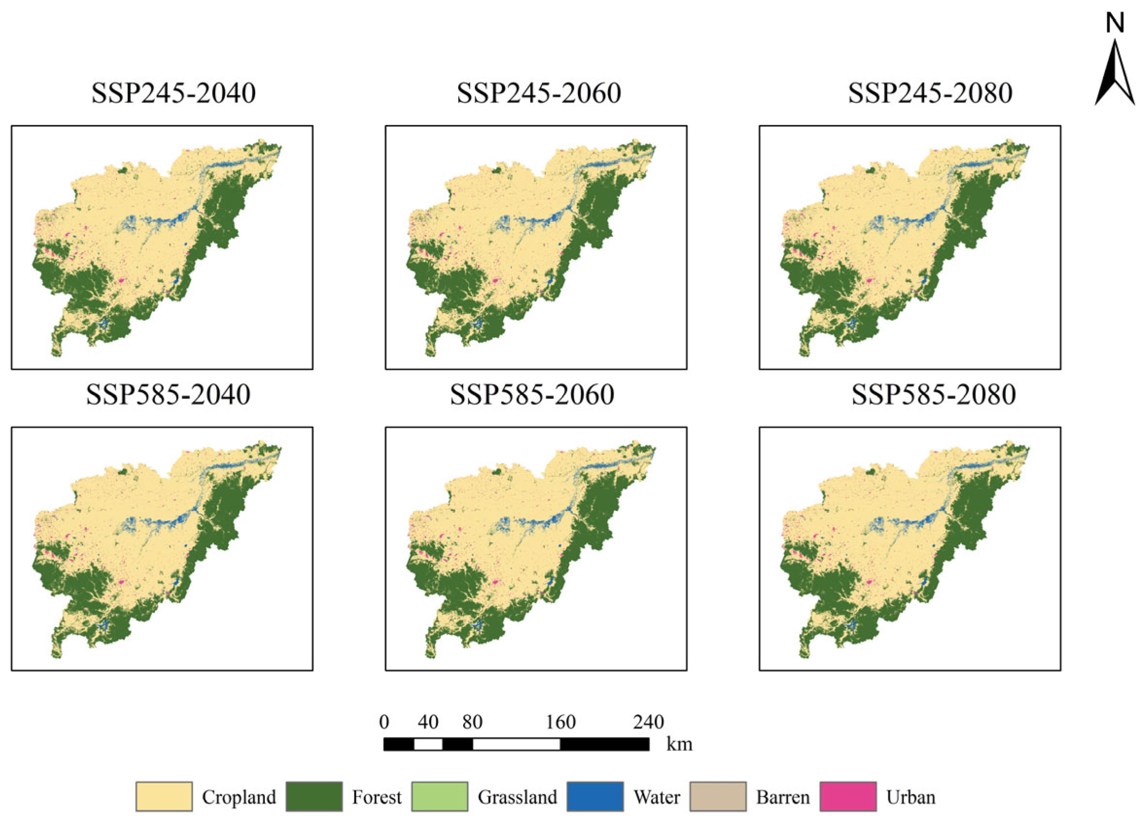
In terms of future land use changes, forest land will continue to grow under different scenarios, while farmland will continue to decline under all scenarios. Water areas will show a significant growth trend under the SSP245 scenario, and construction land will see a gradual increase in area under the SSP585 scenario.

(3)

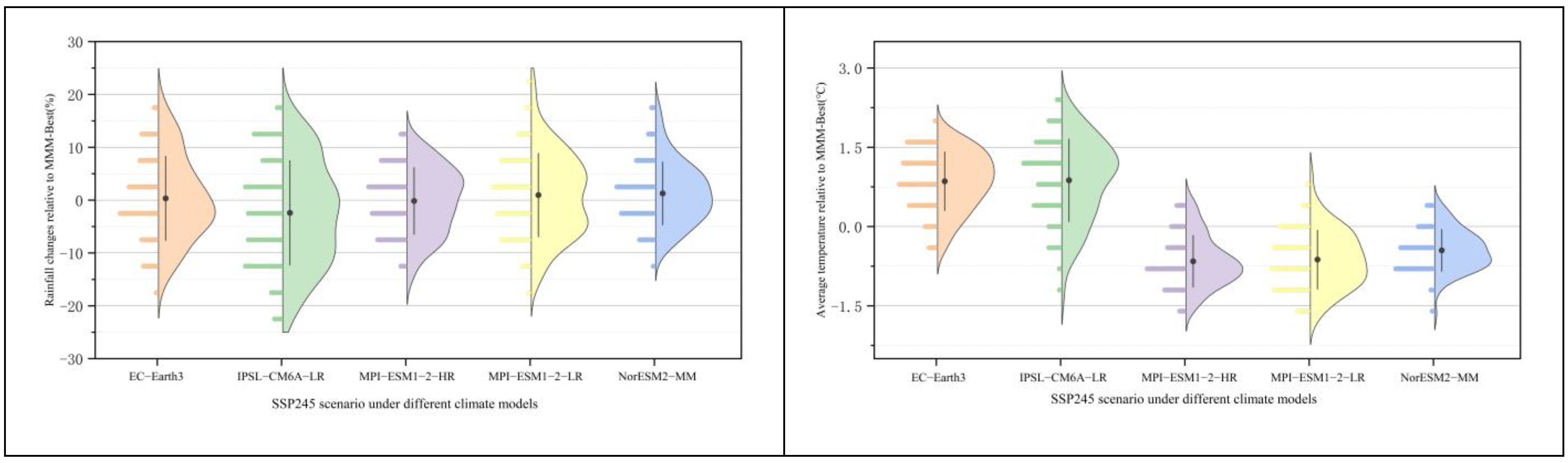
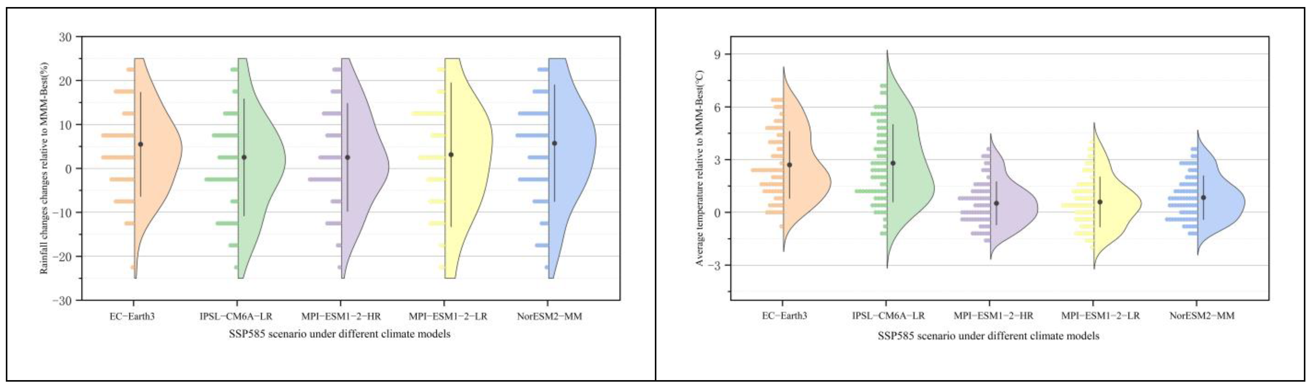
A total of 15 CMIP6 models provided reliable temperature predictions for the Rao River Basin from 1970 to 2014 (r > 0.97, RMSE < 2.98). The models with the best performance were the EC-Earth3, IPSL-CM6A-LR, MPI-ESM1–2-HR, and MPI-ESM1–2-LR. NorESM2-MM performed excellently in precipitation predictions (r > 0.75, RMSE < 30.99, standard deviation ≈ 41.28), with their ensemble average MMM-Best (r = 0.80, RMSE = 26.15) being the best model for predictions from 2025 to 2100. Deviation analysis shows that the EC-Earth3 exhibits the largest deviations under the SSP245 and SSP585 scenarios, with high prediction uncertainty; IPSL-CM6A-LR and NorESM2-MM are the most stable, consistent with MMM-Best, and the NorESM2-MM has the smallest deviation and most conservative predictions under the SSP585 scenario.

(4)

For the years 2025–2100, precipitation, temperature, and runoff in the basin are higher than historical levels under both scenarios. Under the SSP245 and SSP585 scenarios, the SRI-1 values indicate a trend toward future climate warming and increased extreme events, with positive values predominating after 2060, particularly during the summer (June–August) with significant positive values (reaching up to 3.34 and 3.66), indicating an increase in high-temperature or drought events. Land use changes mitigate SRI-1 fluctuations in the SSP245 scenario (−3.62 to 3.34), but the mitigating effect is limited in the SSP585 scenario, with slightly increased positive values (peaking at 3.66). Seasonal analysis shows that positive values are more frequent in summer, while winter and spring are dominated by negative values, with greater intensity in the high-emission scenario (SSP585).

(5)

Under the SSP245 and SSP585 scenarios, hydrological drought (SRI-12) in the Naoli River Basin from 2025 to 2100 shows increased frequency and duration under SSP585. Land use changes have a minimal impact on drought frequency from 2025 to 2040, reduce events from 2041 to 2060 (SSP245: 7 to 4; SSP585: 5 to 4), and increase events from 2061 to 2100 (SSP245: 11 to 14; SSP585: 12 to 15), while shortening long-term drought duration (SSP245: 11.3 to 10.43 months; SSP585: 15.3 to 13.1 months). Land use mitigates drought in the medium to long term, but its effect is limited under high-emission scenarios.

(6)

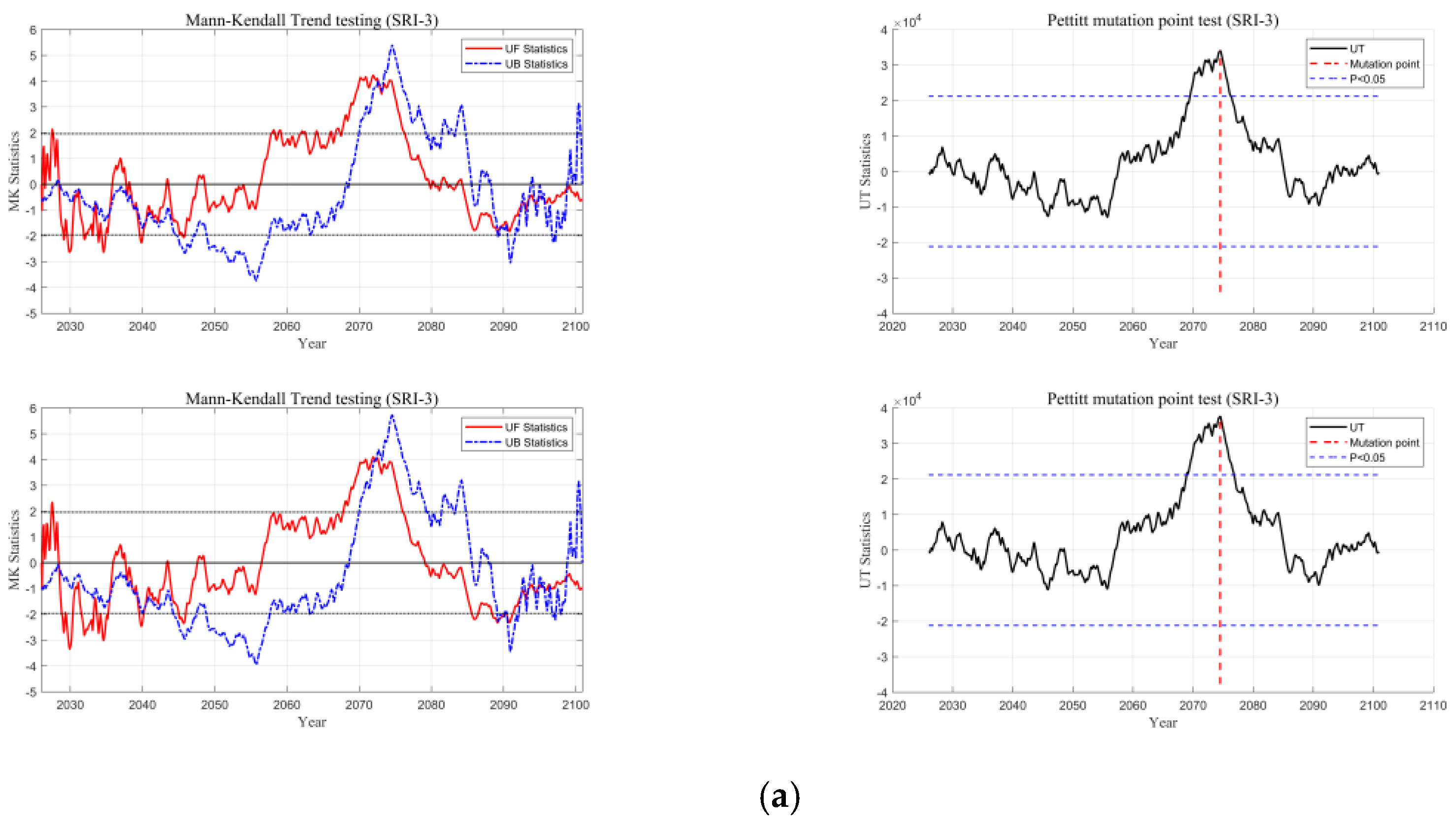
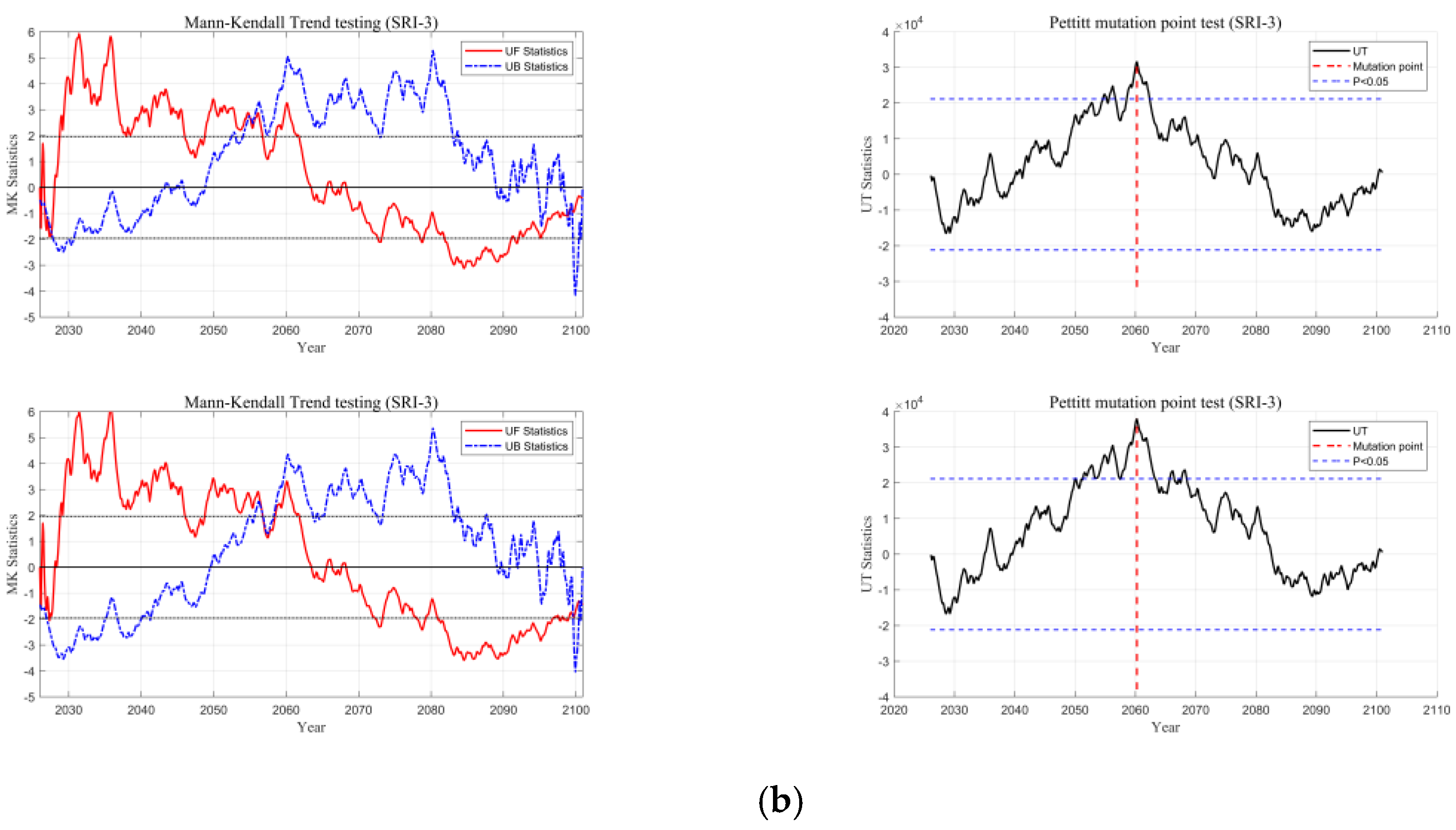
The Pettitt test showed that the SRI-3 mutation point was July 2074 under the SSP245 scenario and April 2060 under the SSP585 scenario (p < 0.05). Land use change had a limited impact on the mutation, with climate drivers being the primary factor, and the mutation occurred earlier under SSP585. The Mann–Kendall test indicated that the trend was highly variable under SSP245, and the number of crossover points increased to 40 after land use change, exacerbating fluctuations; under SSP585, the trend remained stable with only seven crossover points, and land use change had a minor impact, with climate signals dominating. The mutation point coincides with the period of significant trends, indicating that fluctuations under SSP245 are influenced by land use, while the high-emission scenario under SSP585 dominates early mutations and the stable trend.

References

1. Wang, Y.; Peng, T.; He, Y.; Singh, V.P.; Lin, Q.; Dong, X.; Fan, T.; Liu, J.; Guo, J.; Wang, G. Attribution analysis of non-stationary hydrological drought using the GAMLSS framework and an improved SWAT model. J. Hydrol. 2023, 627, 130420. [Google Scholar] [CrossRef]
2. Kiprotich, P.; Wei, X.; Zhang, Z.; Ngigi, T.; Qiu, F.; Wang, L. Assessing the impact of land use and climate change on surface runoff response using gridded observations and swat+. Hydrology 2021, 8, 48. [Google Scholar] [CrossRef]
3. Lukas, P.; Melesse, A.M.; Kenea, T.T. Integrating Land Use/Land Cover and Climate Change Projections to Assess Future Hydrological Responses: A CMIP6-Based Multi-Scenario Approach in the Omo–Gibe River Basin, Ethiopia. Climate 2025, 13, 51. [Google Scholar] [CrossRef]
4. Abdelmoaty, H.M.; Papalexiou, S.M.; Rajulapati, C.R.; AghaKouchak, A. Biases beyond the mean in CMIP6 extreme precipitation: A global investigation. Earth’s Future 2021, 9, e2021EF002196. [Google Scholar] [CrossRef]
5. Fredriksen, H.B.; Smith, C.J.; Modak, A.; Rugenstein, M. 21st century scenario forcing increases more for CMIP6 than CMIP5 models. Geophys. Res. Lett. 2023, 50, e2023GL102916. [Google Scholar] [CrossRef]
6. Wei, S.; Wang, X.; Liu, L.; Qie, L.; Li, Y.; Wang, Q.; Wang, T.; Wang, J.; Gou, X.; Yang, M. Bias correction of CMIP6 GCMs for historical and future air temperatures across China. Atmos. Res. 2025, 323, 108193. [Google Scholar] [CrossRef]
7. DeGuzman, K.; Knappenberger, T.; Brantley, E.; Olshansky, Y. Estimating runoff probability from precipitation data: A binomial regression analysis. Hydrol. Process. 2023, 37, e15029. [Google Scholar] [CrossRef]
8. Yi, S.; Saemian, P.; Sneeuw, N.; Tourian, M.J. Estimating runoff from pan-Arctic drainage basins for 2002–2019 using an improved runoff-storage relationship. Remote Sens. Environ. 2023, 298, 113816. [Google Scholar] [CrossRef]
9. Wu, Q.; Xie, T.; Liu, C.; Li, W.; Zhang, L.; Ran, G.; Xu, Y.; Tang, Y.; Han, Z.; Hu, C. Improving the understanding of rainfall-runoff processes: Temporal dynamic of event runoff response in Loess Plateau, China. J. Environ. Manag. 2025, 375, 123436. [Google Scholar] [CrossRef]
10. Nepal, D.; Parajuli, P.B.; Ouyang, Y.; To, S.F.; Wijewardane, N. Assessing hydrological and water quality responses to dynamic landuse change at watershed scale in Mississippi. J. Hydrol. 2023, 625, 129983. [Google Scholar] [CrossRef]
11. Shrestha, S.; Bhatta, B.; Talchabhadel, R.; Virdis, S.G.P. Integrated assessment of the landuse change and climate change impacts on the sediment yield in the Songkhram River Basin, Thailand. Catena 2022, 209, 105859. [Google Scholar] [CrossRef]
12. Kang, X.; Qi, J.; Bourque, C.P.-A.; Li, S.; Jin, C.; Meng, F.-R. Assessing watershed-scale impacts of best management practices and elevated atmospheric carbon dioxide concentrations on water yield. Sci. Total Environ. 2024, 926, 171629. [Google Scholar] [CrossRef]
13. Zhang, X.; Qi, Y.; Li, H.; Wang, X.; Yin, Q. Assessing the response of non-point source nitrogen pollution to land use change based on SWAT model. Ecol. Indic. 2024, 158, 111391. [Google Scholar] [CrossRef]
14. Yonaba, R.; Biaou, A.C.; Koïta, M.; Tazen, F.; Mounirou, L.A.; Zouré, C.O.; Queloz, P.; Karambiri, H.; Yacouba, H. A dynamic land use/land cover input helps in picturing the Sahelian paradox: Assessing variability and attribution of changes in surface runoff in a Sahelian watershed. Sci. Total Environ. 2021, 757, 143792. [Google Scholar] [CrossRef] [PubMed]
15. Yonaba, R.; Mounirou, L.A.; Tazen, F.; Koïta, M.; Biaou, A.C.; Zouré, C.O.; Queloz, P.; Karambiri, H.; Yacouba, H. Future climate or land use? Attribution of changes in surface runoff in a typical Sahelian landscape. C. R. Géosci. 2023, 355, 411–438. [Google Scholar] [CrossRef]
16. Winkler, K.; Fuchs, R.; Rounsevell, M.; Herold, M. Global land use changes are four times greater than previously estimated. Nat. Commun. 2021, 12, 2501. [Google Scholar] [CrossRef]
17. Yu, H.; Wang, L.; Zhang, J.; Chen, Y. A global drought-aridity index: The spatiotemporal standardized precipitation evapotranspiration index. Ecol. Indic. 2023, 153, 110484. [Google Scholar] [CrossRef]
18. Tahir, Z.; Haseeb, M.; Mahmood, S.A.; Batool, S.; Abdullah-Al-Wadud, M.; Ullah, S.; Tariq, A. Predicting land use and land cover changes for sustainable land management using CA-Markov modelling and GIS techniques. Sci. Rep. 2025, 15, 3271. [Google Scholar] [CrossRef]
19. Jiang, J.; Wang, Z.; Lai, C.; Wu, X.; Chen, X. Climate and landuse change enhance spatio-temporal variability of Dongjiang river flow and ammonia nitrogen. Sci. Total Environ. 2023, 867, 161483. [Google Scholar] [CrossRef]
20. Guédé, K.G.; Yu, Z.; Simonovic, S.P.; Gu, H.; Emani, G.F.; Badji, O.; Chen, X.; Sika, B.; Adiaffi, B. Combined effect of landuse/landcover and climate change projection on the spatiotemporal streamflow response in cryosphere catchment in the Tibetan Plateau. J. Environ. Manag. 2025, 376, 124353. [Google Scholar] [CrossRef]
21. Lv, K.; Si, Z.; Ren, W.; Zhao, Z. Exploring ecosystem services dynamics and interactions under future climate change: A case study of the city cluster in the middle reaches of the Yangtze River. Ecol. Front. 2025, 45, 719–739. [Google Scholar] [CrossRef]
22. Yao, Y.; Wang, L.; Lv, X.; Yu, H.; Li, G. Changes in stream peak flow and regulation in Naoli river watershed as a result of wetland loss. Sci. World J. 2014, 2014, 209547. [Google Scholar] [CrossRef] [PubMed]
23. Pan, T.; Bao, Z.; Ning, L.; Tong, S. Change of rice paddy and its impact on human well-being from the perspective of land surface temperature in the northeastern Sanjiang plain of China. Int. J. Environ. Res. Public Health 2022, 19, 9690. [Google Scholar] [CrossRef]
24. Liu, Z.; Lu, X.; Yonghe, S.; Zhike, C.; Wu, H.; Zhao, Y. Hydrological evolution of wetland in Naoli River Basin and its driving mechanism. Water Resour. Manag. 2012, 26, 1455–1475. [Google Scholar] [CrossRef]
25. Du, X.; Chang, K.; Lu, X. Characteristics and causes of groundwater dynamic changes in Naoli River Plain, Northeast China. Water Supply 2020, 20, 2603–2615. [Google Scholar] [CrossRef]
26. Tang, J.; Li, Y.; Fu, B.; Jin, X.; Yang, G.; Zhang, X. Spatial–temporal changes in the degradation of marshes over the past 67 years. Sci. Rep. 2022, 12, 6070. [Google Scholar] [CrossRef]
27. Bai, X.; Wang, B.; Qi, Y. The effect of returning farmland to grassland and coniferous forest on watershed runoff—A case study of the Naoli River Basin in Heilongjiang Province, China. Sustainability 2021, 13, 6264. [Google Scholar] [CrossRef]
28. Wu, Y.; Sun, J.; Blanchette, M.; Rousseau, A.N.; Xu, Y.J.; Hu, B.; Zhang, G. Wetland mitigation functions on hydrological droughts: From drought characteristics to propagation of meteorological droughts to hydrological droughts. J. Hydrol. 2023, 617, 128971. [Google Scholar] [CrossRef]
29. Yildirim, I.; Aksoy, H.; Hrachowitz, M. Formative drought rate to quantify propagation from meteorological to hydrological drought. Hydrol. Process. 2024, 38, e15229. [Google Scholar] [CrossRef]
30. Ma, Q.; Li, Y.; Liu, F.; Feng, H.; Biswas, A.; Zhang, Q. SPEI and multi-threshold run theory based drought analysis using multi-source products in China. J. Hydrol. 2023, 616, 128737. [Google Scholar] [CrossRef]
31. Chi, G.; Zhu, B.; Huang, B.; Chen, X.; Shi, Y. Spatiotemporal dynamics in soil iron affected by wetland conversion on the Sanjiang Plain. Land Degrad. Dev. 2021, 32, 4669–4679. [Google Scholar] [CrossRef]
32. Zhang, Z.; Yang, M.; Li, L.; Yin, R.; Huo, L. Holocene terrestrialization process on the Sanjiang Plain (China) and its significance to the East Asian summer monsoon circulation. Sci. Total Environ. 2022, 806, 150578. [Google Scholar] [CrossRef] [PubMed]
33. Xu, C.; Zhang, Z.; Fu, Z.; Xiong, S.; Chen, H.; Zhang, W.; Wang, S.; Zhang, D.; Lu, H.; Jiang, X. Impacts of climatic fluctuations and vegetation greening on regional hydrological processes: A case study in the Xiaoxinganling Mountains–Sanjiang Plain region, Northeastern China. Remote Sens. 2024, 16, 2709. [Google Scholar] [CrossRef]
34. Luo, C.; Fu, X.; Zeng, X.; Cao, H.; Wang, J.; Ni, H.; Qu, Y.; Liu, Y. Responses of remnant wetlands in the Sanjiang Plain to farming-landscape patterns. Ecol. Indic. 2022, 135, 108542. [Google Scholar] [CrossRef]
35. Wu, Y.; Xu, N.; Wang, H.; Li, J.; Zhong, H.; Dong, H.; Zeng, Z.; Zong, C. Variations in the diversity of the soil microbial community and structure under various categories of degraded wetland in Sanjiang Plain, northeastern China. Land Degrad. Dev. 2021, 32, 2143–2156. [Google Scholar] [CrossRef]
36. Zhang, L.; Nan, Z.; Yu, W.; Ge, Y. Modeling land-use and land-cover change and hydrological responses under consistent climate change scenarios in the Heihe River Basin, China. Water Resour. Manag. 2015, 29, 4701–4717. [Google Scholar] [CrossRef]
37. Ma, L.; Liu, J.; Pang, X.; Jing, H. Analysis of Hydrological Elements and Runoff Prediction in Tao′er River Basin under Land Use and Climate Change. J. Soil Water Conserv. 2025, 39, 1009–2242. [Google Scholar]
38. Long, S.; Gao, J.; Shao, H.; Wang, L.; Zhang, X.; Gao, Z. Developing SWAT-S to strengthen the soil erosion forecasting performance of the SWAT model. Land Degrad. Dev. 2024, 35, 280–295. [Google Scholar] [CrossRef]
39. Huang, C.; Zhang, Y.; Hou, J. Soil and Water Assessment Tool (SWAT)-informed deep learning for streamflow forecasting with remote sensing and in situ precipitation and discharge observations. Remote Sens. 2024, 16, 3999. [Google Scholar] [CrossRef]
40. Wang, Z.; He, Y.; Li, W.; Chen, X.; Yang, P.; Bai, X. A generalized reservoir module for SWAT applications in watersheds regulated by reservoirs. J. Hydrol. 2023, 616, 128770. [Google Scholar] [CrossRef]
41. Valencia, S.; Villegas, J.C.; Hoyos, N.; Duque-Villegas, M.; Salazar, J.F. Streamflow response to land use/land cover change in the tropical Andes using multiple SWAT model variants. J. Hydrol. Reg. Stud. 2024, 54, 101888. [Google Scholar] [CrossRef]
42. Melaku, N.D.; Brown, C.W.; Tavakoly, A.A. Improving process-based prediction of stream water temperature in SWAT using semi-Lagrangian formulation. J. Hydrol. 2025, 651, 132612. [Google Scholar] [CrossRef]
43. Cao, K.; Liu, X.; Fu, Q.; Wang, Y.; Liu, D.; Li, T.; Li, M. Dynamic and harmonious allocation of irrigation water resources under climate change: A SWAT-based multi-objective nonlinear framework. Sci. Total Environ. 2023, 905, 167221. [Google Scholar] [CrossRef]
44. Zabihi, O.; Ahmadi, A. Multi-criteria evaluation of CMIP6 precipitation and temperature simulations over Iran. J. Hydrol. Reg. Stud. 2024, 52, 101707. [Google Scholar] [CrossRef]
45. Mesgari, E.; Hosseini, S.A.; Hemmesy, M.S.; Houshyar, M.; Partoo, L.G. Assessment of CMIP6 models’ performances and projection of precipitation based on SSP scenarios over the MENAP region. J. Water Clim. Change 2022, 13, 3607–3619. [Google Scholar] [CrossRef]
46. Zhang, Z.; Duan, K.; Liu, H.; Meng, Y.; Chen, R. Spatio-temporal variation of precipitation in the Qinling mountains from 1970 to 2100 based on CMIP6 data. Sustainability 2022, 14, 8654. [Google Scholar] [CrossRef]
47. Guo, W.; Yu, L.; Huang, L.; He, N.; Chen, W.; Hong, F.; Wang, B.; Wang, H. Ecohydrological response to multi-model land use change at watershed scale. J. Hydrol. Reg. Stud. 2023, 49, 101517. [Google Scholar] [CrossRef]
48. Li, C.; Wu, Y.; Gao, B.; Zheng, K.; Wu, Y.; Li, C. Multi-scenario simulation of ecosystem service value for optimization of land use in the Sichuan-Yunnan ecological barrier, China. Ecol. Indic. 2021, 132, 108328. [Google Scholar] [CrossRef]
49. Wang, R.; Zhao, J.; Chen, G.; Lin, Y.; Yang, A.; Cheng, J. Coupling PLUS–InVEST model for ecosystem service research in Yunnan Province, China. Sustainability 2022, 15, 271. [Google Scholar] [CrossRef]
50. Lin, X.; Jiao, X.; Tian, Z.; Sun, Q.; Zhang, Y.; Zhang, P.; Ji, Z.; Chen, L.; Lun, F.; Chang, X.; et al. Projecting diversity conflicts of future land system pathways in China under anthropogenic and climate forcing. Earth’s Future 2023, 11, e2022EF003406. [Google Scholar] [CrossRef]
51. Van Vuuren, D.P.; Riahi, K.; Calvin, K.; Dellink, R.; Emmerling, J.; Fujimori, S.; Kc, S.; Kriegler, E.; O’Neill, B. The Shared Socio-economic Pathways: Trajectories for human development and global environmental change. Glob. Environ. Change 2017, 42, 148–152. [Google Scholar] [CrossRef]
52. Rajwa-Kuligiewicz, A.; Bojarczuk, A. Streamflow response to catastrophic windthrow and forest recovery in subalpine spruce forest. J. Hydrol. 2024, 634, 131078. [Google Scholar] [CrossRef]
53. Baez-Villanueva, O.M.; Zambrano-Bigiarini, M.; Miralles, D.G.; Beck, H.E.; Siegmund, J.F.; Alvarez-Garreton, C.; Verbist, K.; Garreaud, R.; Boisier, J.P.; Galleguillos, M. On the timescale of drought indices for monitoring streamflow drought considering catchment hydrological regimes. Hydrol. Earth Syst. Sci. 2024, 28, 1415–1439. [Google Scholar] [CrossRef]
54. Wu, J.; Chen, X.; Yao, H.; Zhang, D. Multi-timescale assessment of propagation thresholds from meteorological to hydrological drought. Sci. Total Environ. 2021, 765, 144232. [Google Scholar] [CrossRef]
55. Wen, L.; Rogers, K.; Ling, J.; Saintilan, N. The impacts of river regulation and water diversion on the hydrological drought characteristics in the Lower Murrumbidgee River, Australia. J. Hydrol. 2011, 405, 382–391. [Google Scholar] [CrossRef]
56. Zhao, X.; Zhang, W.; Feng, Y.; Mo, Q.; Su, Y.; Njoroge, B.; Qu, C.; Gan, X.; Liu, X. Soil organic carbon primarily control the soil moisture characteristic during forest restoration in subtropical China. Front. Ecol. Evol. 2022, 10, 1003532. [Google Scholar] [CrossRef]
57. Zhang, L.; Nan, Z.; Yu, W.; Ge, Y. Hydrological responses to land-use change scenarios under constant and changed climatic conditions. Environ. Manag. 2016, 57, 412–431. [Google Scholar] [CrossRef]
58. Liu, J.; Wang, S.-Y.; Li, D.-M. The analysis of the impact of land-use changes on flood exposure of Wuhan in Yangtze River Basin, China. Water Resour. Manag. 2014, 28, 2507–2522. [Google Scholar] [CrossRef]
59. Chen, S.; Li, X.; Qian, Z.; Wang, S.; Wang, M.; Liu, Z.; Li, H.; Xia, H.; Zhao, Z.; Li, T.; et al. Drought trend and its impact on ecosystem carbon sequestration in Lancang-Mekong River Basin. Acta Geogr. Sin. 2024, 79, 747–764. [Google Scholar]
60. IPCC. Climate Change 2021: The Physical Science Basis. Contribution of Working Group I to the Sixth Assessment Report of the Intergovernmental Panel on Climate Change; Masson-Delmotte, V., Zhai, P., Pirani, A., Connors, S.L., Péan, C., Berger, S., Caud, N., Chen, Y., Goldfarb, L., Gomis, M., et al., Eds.; Cambridge University Press: Cambridge, UK; New York, NY, USA, 2021. [Google Scholar]
61. Yang, S.; Wang, H.; Tong, J.; Bai, Y.; Alatalo, J.M.; Liu, G.; Fang, Z.; Zhang, F. Impacts of environment and human activity on grid-scale land cropping suitability and optimization of planting structure, measured based on the MaxEnt model. Sci. Total Environ. 2022, 836, 155356. [Google Scholar] [CrossRef]
62. Deng, X.; Zhang, Q.; Sun, P.; Fang, C. Assessment of impacts of climate change and human activities on runoff with HSPF for the Xinjiang River Basin. Trop. Geogr. 2014, 34, 293–301. [Google Scholar]
Figure 1. Distribution of water systems and locations of hydrometeorological stations in the Naoli River Basin.
Water 17 01696 g001
Figure 2. Research framework diagram.
Water 17 01696 g002
Figure 3. Simulation results of the Naoli River Basin model.
Water 17 01696 g003
Figure 4. Taylor diagram of rainfall, maximum temperature, and minimum temperature in the Niao River basin simulated by CMIP6 from 1970 to 2014 relative to the observation site.
Water 17 01696 g004
Figure 5. Analysis of meteorological model and integrated mean model biases under SSP245 and SSP585 scenarios.
Water 17 01696 g005aWater 17 01696 g005b
Figure 6. Land use Sankey diagram from 2000 to 2020. Note: Fig. shows only the changes in land use types.
Water 17 01696 g006
Figure 7. SSP typical scenario land use prediction distribution.
Water 17 01696 g007
Figure 8. Analysis of the temporal impact of land use and climate change on runoff.
Water 17 01696 g008
Figure 9. SRI maps of land use and future climate for different scenarios.
Water 17 01696 g009
Figure 10. Trends and sudden changes in land use before and after different scenarios. (a) MK test and p-value inflection points before and after land use in the SSP245 scenario. (b) MK test and p-value inflection points before and after land use in the SSP585 scenario.
Water 17 01696 g010aWater 17 01696 g010b