Temporal and Spatial Analysis of Deformation and Instability, and Trend Analysis of Step Deformation Landslide

Abstract

This study focuses on step deformation landslides, conducting spatiotemporal analysis of landslide deformation and instability trends. First, the target landslide area is selected, and geological and precipitation data, along with historical displacement data from monitoring points, are collected. The slope single-change-point analysis method is then employed, combined with landslide profile data, to extract key features from the monitoring data. Next, Small BAseline Subset-Interferometric Synthetic Aperture Radar (SBAS-InSAR) technology is applied to obtain satellite images of the study area. These images, together with the extracted data features, are used to draw the spatiotemporal baseline of the target landslide, completing the spatiotemporal analysis. Finally, a landslide prediction model is developed, and its prediction error is corrected using an Extreme Learning Machine (ELM) neural network. The refined prediction results serve as the basis for analyzing the landslide deformation coefficient, enabling the determination of the landslide instability trend. The experimental results show that step deformation landslides exhibit significant spatiotemporal variability and a short stability period throughout the year. The analytical methods designed in this study outperform traditional methods, providing more reliable results for predicting landslide instability trends.

1. Introduction

Research on geological hazard prevention and control shows that landslides, as a typical type of geological hazard, exhibit unique evolutionary characteristics in complex geological environments [1]. The deformation process of disaster bodies represented by step landslides often has a significant coupling relationship with drastic changes in the hydrological environment and has multi-stage and abrupt movement characteristics. Under the influence of external factors such as heavy rainfall or changes in reservoir water level, this type of landslide often undergoes dynamic adjustments in the seepage pressure field [2], leading to a weakening of the landslide’s shear strength and triggering displacement step responses.

The evolution process of step deformation landslides can be deconstructed into a cyclic pattern of “stress accumulation, critical instability, energy release”. Monitoring data shows that over 80% of sudden displacement events are synchronized with short-term heavy rainfall processes, with a significant increase in triggering probability when the water level rise and fall rate exceeds 2 m/d [3,4]. This nonlinear deformation mechanism leads to a lag in the traditional displacement rate threshold method for early warning, especially in areas where multiple periods of step stacking occur, and the cumulative effect of deformation may cause sudden changes in disaster characteristics.

The spatiotemporal characteristics of landslide deformation are a critical foundation for analyzing the mechanism of landslide disasters and evaluating disaster risks. Although existing detection technologies meet temporal and spatial requirements, there remains a gap in addressing the increasingly sophisticated requirements for landslide prediction. In previous studies, various landslide prediction models have been proposed. Since the 1960s, these models have undergone decades of research and exploration, gradually evolving into various methodologies and being applied to landslide detection work. For example, reference [5] proposed a method for monitoring landslides using Sentinel-2 satellite images. This approach attempted to automatically map slow-moving landslides using the feature tracking of free and globally available optical satellite images through remote sensing workflows. While this method can monitor landslides, it relies on tracking the temporal characteristics of optical images. However, this method relies too much on the temporal feature tracking of optical images, which makes it susceptible to interference from factors such as cloud cover and seasonal vegetation changes, resulting in significant accumulation of displacement field calculation errors. Especially in low-texture areas, the success rate of feature point matching is low, the spatial resolution is insufficient, and it is difficult to capture local micro deformations, which reduces the analysis reliability of this method. In reference [6], an improved Graph Convolutional Network, GCN, was applied to analyze SAR images, enabling deformation monitoring and overall trend prediction of landslides. Although the improved graph convolutional network has improved the efficiency of deformation extraction in SAR images, the landslide development process has significant temporal evolution characteristics. The improved GCN still uses static graph convolution kernels, which do not have time nonlinearity, making it difficult to model displacement rates, resulting in poor accuracy of this method for landslide deformation analysis. The deformation characteristics of the Kadui-2 landslide under the influence of water storage depth reduction and precipitation were studied in reference [7]. A three-year monitoring project was implemented to observe short-term/long-term deformation. During this period, the landslide experienced continuous deformation. Based on the recorded data on reservoir water level and precipitation during this period, this study established a two-dimensional finite element model using Geostudio software to simulate deformation under different conditions. This research aimed to understand the actual impact of these triggering factors on landslides. Through numerical simulation, it was found that the maximum deformation occurs on the front side of the landslide. As the long-term shear strength gradually decreases, the sliding surface exhibits obvious creep characteristics. The fluctuation in reservoir water level was the main triggering factor for the revival of landslide bodies, with a negative correlation to the deformation rate. In contrast, rainfall, due to limited surface infiltration, showed no significant impact on the sliding motion of landslides compared to reservoir water storage and depth reduction operations. However, the two-dimensional finite element model has inherent flaws, as it ignores the lateral boundary constraint effect when simplifying three-dimensional landslides as plane strain problems, resulting in overestimation of the deformation of the leading edge and affecting the accuracy of this method for landslide deformation analysis.

The deformation behavior of step landslides is governed by the coupling effect of multiple physical fields. From a mechanical perspective, the dynamic weakening of the shear strength of the sliding band is the primary cause of step displacement. Under conditions of a sudden drop in reservoir water level or heavy rainfall, the seepage field inside the sliding body undergoes drastic adjustments. This leads to an increase in pore water pressure gradient and a decrease in effective stress. When the shear stress of the sliding soil exceeds its residual strength, the sliding body enters the accelerated deformation stage. In addition, the redistribution of internal stress in the sliding body can cause strain localization, forming shear bands that gradually expand. This process ultimately manifests as a step-like abrupt change in surface displacement. Considering the diverse triggering factors behind step deformation landslides, this study proposes a more refined temporal and spatial analysis of deformation and instability trend analysis of step deformation landslides. In this study, firstly, geological, precipitation, and historical displacement data of the target landslide were collected to construct a data foundation. Subsequently, key feature points were extracted using the slope single-change-point analysis method to grasp the stage specific characteristics of landslide deformation. To analyze the spatiotemporal characteristics of landslide deformation, this study adopts Small BAseline Subset-Interferometric Synthetic Aperture Radar (SBAS-InSAR) technology, which can effectively reduce atmospheric and topographic errors, generate high-precision deformation data, draw spatiotemporal baseline maps, and provide support for understanding the long-term trends and short-term fluctuations in landslides. In the construction of the prediction model, this study introduces an Extreme Learning Machine (ELM) neural network to correct prediction errors. The ELM network has fast learning and good generalization ability, which can effectively handle nonlinear features in landslide deformation data and improve prediction accuracy. Finally, based on the revised prediction results, the trend of landslide instability is analyzed, the variation law of the deformation coefficient is determined, and a scientific basis for landslide disaster prevention and control is provided.

2. Overview and Data of Landslides in the Research Area

The target landslide in this study is a landslide site located in a reservoir area in southeastern China. It spans approximately 2000 m in length and 1500 m in width. The landslide has a horseshoe-shaped planar outline, with its movement direction oriented from west to east. A specific ditch marks its eastern node, while a certain stone ditch defines its western boundary. The specific landslide range is shown in Figure 1.

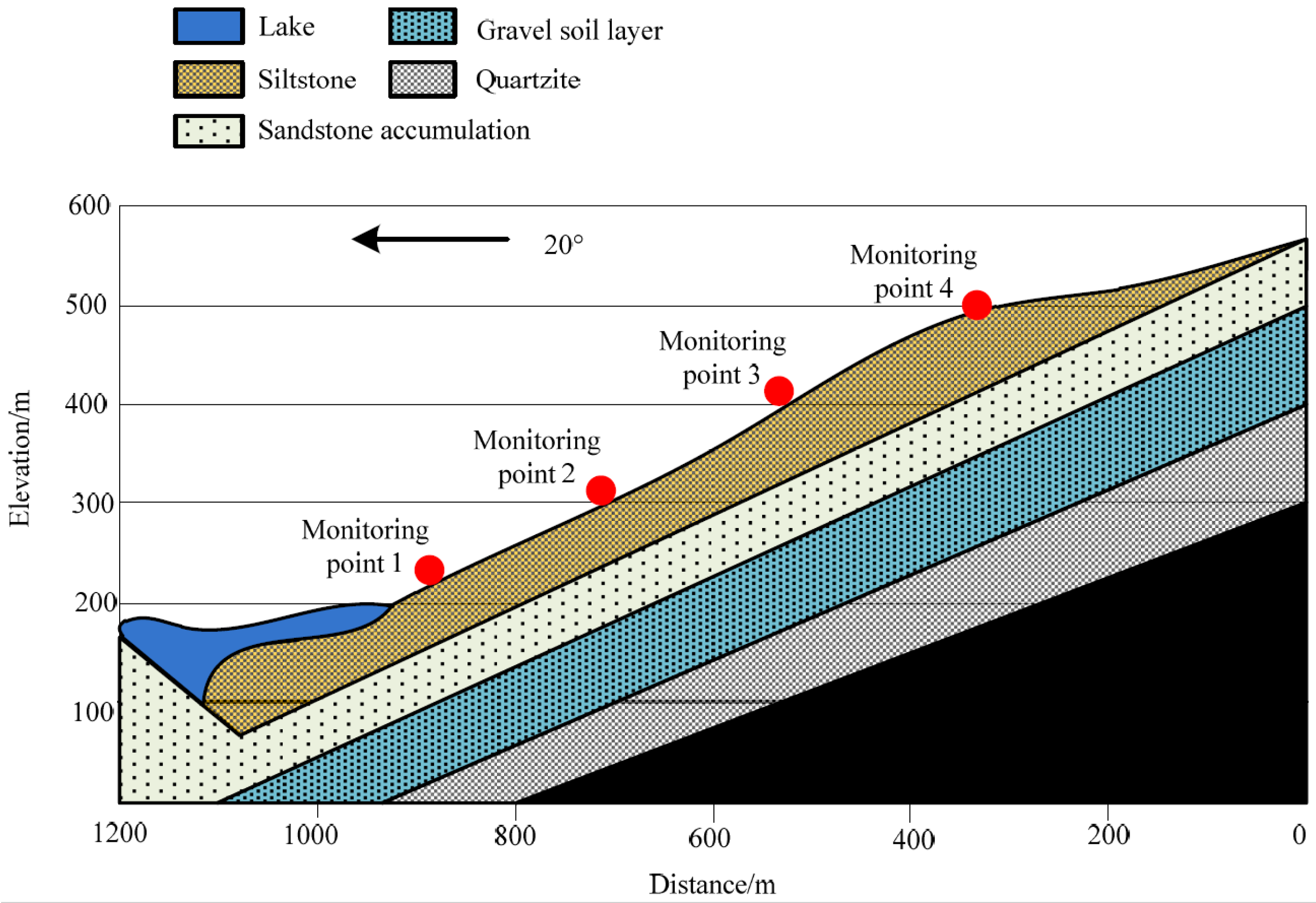
As shown in Figure 1, this landslide is a monocline structure with a dip angle ranging from 10° to 15°, accompanied by wide and gentle folds and minor faults, with some strata having a dip angle exceeding 15°. The overall terrain is higher in the west and lower in the east, with an altitude ranging from 755.60 m to 796.40 m and a maximum altitude drop of 41.00 m. The micro terrain includes river terraces, mountain slopes, etc., showing a stepped distribution, with dense vegetation mainly consisting of pine trees and dwarf shrubs. The main body of the area consists of clay, gravel, and silty clay. The geological composition of this area is shown in Figure 2.

As shown in Figure 2, four fully automatic surface-displacement-monitoring devices were installed on this landslide to obtain more accurate landslide data. According to the topographic profile map, the upper part of the landslide has a similar inclination angle to the rock surface and is in a straight-line shape. At the same time, the overall trend of the lower sliding bed is relatively gentle. The sliding body is composed of two distinct layers: the upper layer is a loose accumulation of body, and the lower layer is composed of quartz sandstone and siltstone. The soil in the front of the landslide contains some gravel, while the rear is a relatively weak coal-bearing stratum.

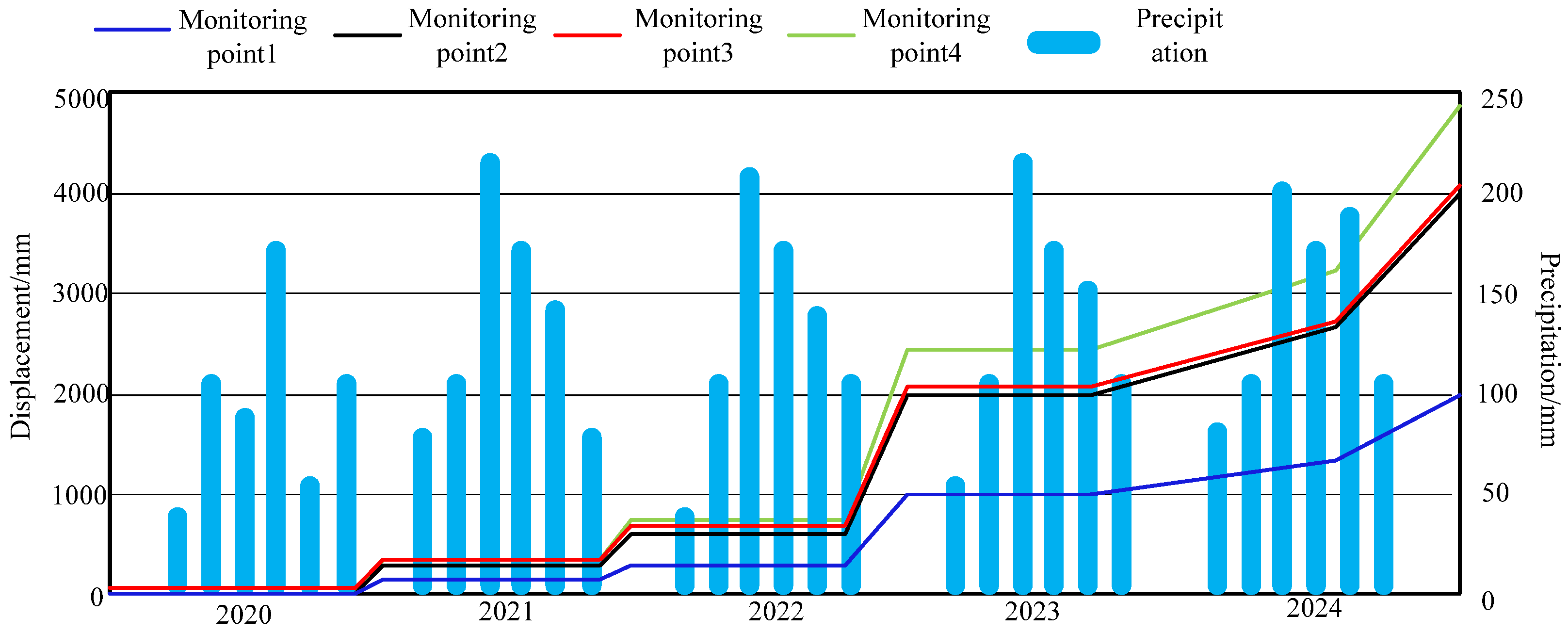
After obtaining data from rainfall-monitoring stations and crack-monitoring devices in the landslide area during the research interval, redundant data are first removed. By comparing duplicate data from different monitoring points and time periods, combined with data quality evaluation indicators, clear duplicate or invalid data records are deleted. Subsequently, error data correction was performed to address data biases caused by instrument errors, environmental interference, and other factors. Median filtering was used to correct the data, ensuring its accuracy and reliability. The landslide displacement precipitation time curve was then plotted, as shown in Figure 3.

As shown in Figure 3, data spanning a total of 5 years of landslide displacement and precipitation were obtained in this study, and these were plotted as images to provide a more concrete data basis for this research. Among them, precipitation data are calculated over a period of 2 months.

The main factors influencing landslides in this area include reservoir water level, precipitation, and human activities. The step deformation characteristics of the target landslide are directly related to its special geological and hydrological conditions. The loose accumulation on the upper layer of the landslide has high permeability. In contrast, the underlying quartz sandstone layer has extremely low permeability, forming a typical “upper permeability and lower isolation” double-layer structure. During the rapid decline in the reservoir’s water level, the upper pore water is rapidly discharged. In contrast, the bottom stagnant water forms reverse osmotic pressure, resulting in a sudden decrease in effective normal stress in the sliding zone. At the same time, the montmorillonite minerals in coal-bearing strata swell when exposed to water, further weakening the shear strength of the slip zone. The synergistic effect of this osmotic pressure difference and mineral expansion causes the sliding body to frequently trigger step deformation, which conforms to the instability mode of strain-controlled landslides.

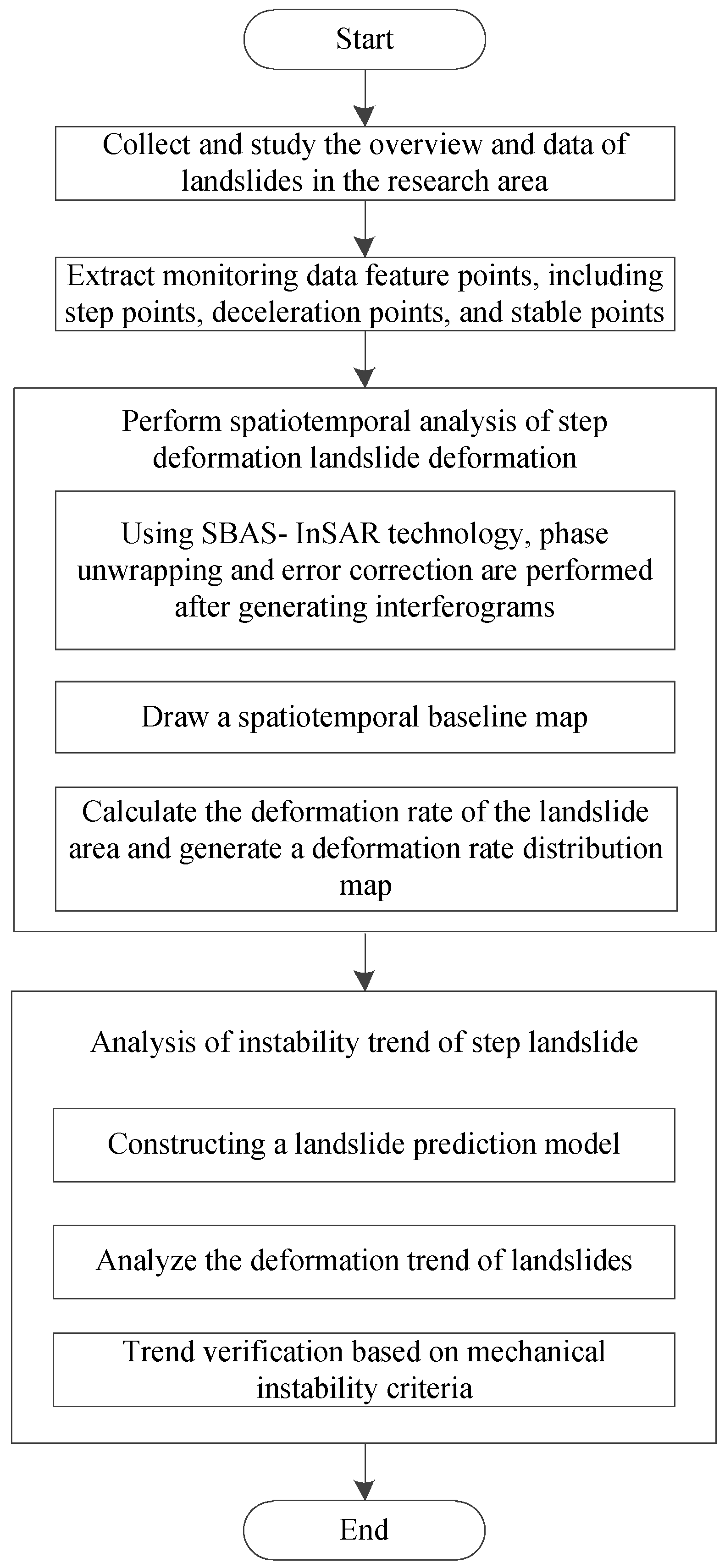
The data above were organized, the target landslide area was analyzed through this part of the data, and based on this, the spatiotemporal analysis of step deformation, landslide deformation, and instability trend analysis was completed. The approach of this study is shown in Figure 4.

3. Extract Monitoring Data Feature Points

3.1. Extraction Process of Monitoring Data Feature Points

To achieve spatiotemporal analysis, it is necessary to process the obtained monitoring data and obtain feature points. Before obtaining the data feature points, based on the analysis results of a large number of files, the basic characteristics of step landslides were summarized, as shown in

Table 1. Characteristics of step landslides.

Feature Point	Step Point	Deceleration Point	Stable Point
Position	Starting point of the acceleration phase, ending point of the constant velocity phase	Acceleration stage central	End point of the acceleration phase, starting point of the constant velocity phase
Speed	Uniform speed towards acceleration	Peak velocity of landslide movement	Slow down gradually towards a constant speed
The influence of external factors on landslides	The influence of external factors is gradually increasing	The influence of external factors gradually decreases	The disappearance of external factors

.

Based on the content of Table 1, the step points, deceleration points, and stability points were set as the required feature points for this analysis. Given that the data collected by monitoring equipment is mostly one-dimensional, discrete data, it is difficult to use the original derivative method for feature point recognition. This study chose the slope single point analysis method [8,9,10] to complete this part of the operation.

The data column $T=\left[t_1,t_2,\dots ,t_i,\dots ,t_{N-1}\right]$ is set, where $T$ represents the midpoint of monitoring data at equal time intervals, and $N$ represents the total number of monitoring data samples. For each $t_i$, a fixed number of data points is taken before and after, a sliding window is formed, and the linear regression coefficients for the first $n$ data points and the last $n$ data points are calculated due to the direct impact of sample size on the overall slope of the regression curve during the calculation process [11,12]. Therefore, by setting the sample size to 3, 4, and 5, forming three sets of sliding windows based on the selection results, and integrating the data obtained from the three sets of sliding windows to obtain a weighted average, we have:

$$\overline{a_j(t_i)}={\displaystyle \frac{\left[3^2\ast a_j^{(3)}(t_i)+4^2\ast a_j^{(4)}(t_i)+5^2\ast a_j^{(5)}(t_i)\right]}{(3^2+4^2+5^2)}}$$

(1)

Among them, $a_j^{(n)}(t_i)$ represents the linear regression coefficient of the last $n$ data points; $a_i^{(n)}(t_i)$ represents the linear regression coefficient of the first $n$ data points [13]. In this process, selecting 3, 4, and 5 as sample sizes is essentially achieved through collaborative analysis of multi-scale windows, balancing sensitivity, stability, and computational efficiency. This design not only conforms to the nonlinear characteristics of landslide deformation data (such as step changes and gradient superposition), but also improves the reliability of feature point extraction through weighted averaging strategy, providing a high-quality data foundation for subsequent spatiotemporal analysis and instability trend prediction.

For each $t_i$, the first-order difference to represent the slope increment in the curve before and after $t_i$ is calculated, and $\Delta C(t_i)$ is used to represent:

$$\Delta C(t_i)=\overline{a_j(t_i)}-\overline{a_i(t_i)}$$

(2)

The calculation results of the above formula are obtained and second-order decomposition is performed to represent the changes in slope acceleration within $(t_{i-1},t_i)$, denoted as ${\Delta }^{2}C(t_i)$:

$${\Delta }^{2}C(t_i)=\Delta C(t_i)-\Delta C(t_{i-1})$$

(3)

Using the above formula, the maximum value of ${\Delta }^{2}C(t_i)$ is obtained and the location of the maximum slope change in the curve is determined [14]. The position $p$ of the slope change point is obtained as follows:

$$p=t_{i-1}+{\displaystyle \frac{\Delta C(t_i)-\Delta C(t_{i-1})}{\left[\Delta C(t_i)-\Delta C(t_{i-1})\right]+\Delta C(t_i)-\Delta C(t_{i-1})}}\ast (t_i-t_{i-1})$$

(4)

The maximum value of all ${\Delta }^{2}C(t_i)$ values corresponding to the set containing stable points and step points is calculated, and the specific feature points based on the positive and negative values of ${\Delta }^{2}C(t_i)$ are determined [15]. Based on previous research experience, this study defines the positive value of ${\Delta }^{2}C(t_i)$ as a step point. The negative value node of ${\Delta }^{2}C(t_i)$ is the stable point.

Due to the inability to calculate the deceleration point using the above content, the calculation process in this study is set as follows:

The displacement velocity obtained by the surface displacement monitoring equipment is set to $V=\left[v_1,v_2,\dots ,v_i,\dots ,v_{N-1}\right]$, which is used as input information; an LMS graph is constructed, and linear castration is performed on this graph. A moving window is used to determine the maximum value of the displacement velocity interval. Setting the length of the moving window to $b_k$, the value of $b_k$ has variability, and the following is obtained:

$$b_k=2k$$

(5)

Among them, $k$ represents the window calculation coefficient, and for its existence:

$$h_{i,k}=\left\{\begin{array}{c}0 v_{i-1}<v_{i-k-1}\cap v_{i+k-1}\hfill \\ o+\alpha otherwise\hfill \end{array}\right.$$

(6)

Among them, $o$ represents a randomly distributed numerical value within the [0, 1] interval; $\alpha$ represents the constant factor required during the calculation process. By comparing the calculation results under different $k$ values, the most suitable calculation window is obtained. To improve computation speed, Formula (6) is integrated into the following matrix:

$$H=\left[\begin{array}{cccc}{h}_{1,1}& h_{1,2}& \dots & h_{1,N}\\ h_{2,1}& h_{2,2}& \dots & h_{2,N}\\ \dots & \dots & \dots & \dots \\ h_{M,1}& h_{M,2}& \dots & h_{M,N}\end{array}\right]=(h_{m,i})$$

(7)

This matrix is summed up to obtain:

$${\varpi }_k={\displaystyle \sum _{i=1}^n{h}_{m,i}}$$

(8)

For the formula above, the size of the value result can be determined through Formula (5), and the most suitable window can be obtained. At the same time, the minimum value of ${\varpi }_k$ is obtained, Formula (6) is reconstructed to obtain $H_i=(h_{m,i})$, and then the final deceleration point is determined through Formula (8):

$${\beta }_i={\displaystyle \frac{{\displaystyle \sum _{k=1}^{\theta }\left[(h_{m,i}-\frac{{\displaystyle \sum _{k=1}^{\theta }{h}_{m,i}}}{\theta })\right]}}{\theta -1}}$$

(9)

Through the process above, the feature point information of the target landslide is obtained and it is used as the data basis for subsequent spatiotemporal analysis.

3.2. Extraction Results of Feature Points in the Target Area

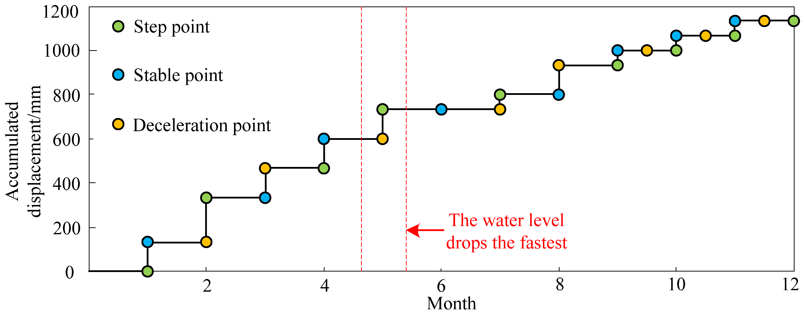
Considering the high overall consistency of the monitoring data obtained by the monitoring equipment, taking 2024 as an example, the data from measuring point 1 can be selected for analysis to obtain the cumulative displacement data for 2024 and complete the analysis process. The feature point recognition results of inputting the data obtained from the monitoring equipment into the algorithm set in the previous text are shown in Figure 5.

Observing Figure 5, it can be seen that since the monitoring of the target landslide, the step period of the landslide is 1 year due to the influence of the reservoir’s water level. During this period, the step points are concentrated in March and April, the deceleration points are concentrated in May and June, and the stable points are concentrated in July and August. From Figure 5, it can be observed that the fastest decline in reservoir water level occurs in May each year, which is consistent with the calculation results obtained from Figure 5. This indicates that Figure 5 has high reliability and can be applied in subsequent spatiotemporal analysis work.

4. Temporal and Spatial Analysis of Deformation in Step Deformation Landslides

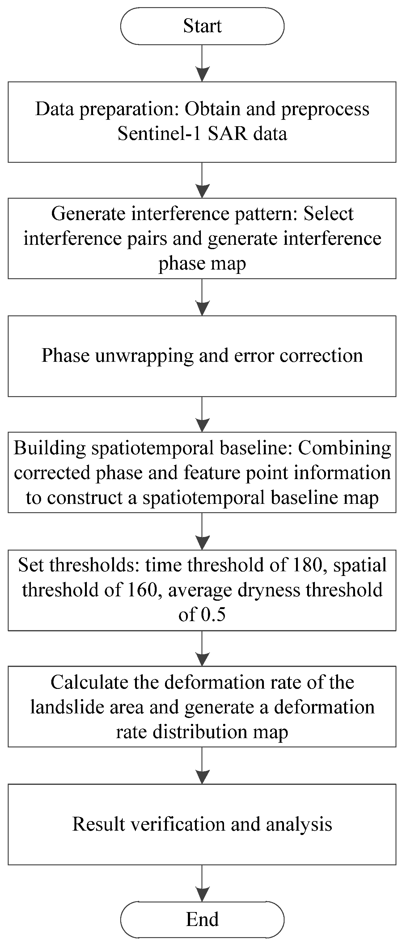
In the spatiotemporal analysis of landslide deformation, this study applies SBAS-InSAR technology to obtain satellite images of the study area, combines the extracted data feature points, draws the spatiotemporal baseline of the target landslide, and completes the spatiotemporal analysis. SBAS-InSAR technology effectively reduces the impact of atmospheric delay and terrain errors by selecting interferometric image pairs with smaller time and spatial baselines, providing broader spatial coverage and higher deformation measurement accuracy. It can handle areas with complex terrain, such as mountains and hills, which is particularly important for the target landslide area in this study. In addition, SBAS-InSAR technology can also generate deformation maps of time series, which helps to better understand the long-term trends and short-term fluctuations in landslide deformation.

4.1. Processing of Characteristic Data of the Step Deformation Landslide

After comparing various technologies, SBAS-InSAR technology [16,17] was chosen as the core technology for spatiotemporal analysis in this study. This technology has comprehensive coverage and can provide more accurate results for spatiotemporal analysis based on the obtained feature point information. Firstly, an appropriate pairing scheme is selected and as many interferograms as possible are generated while minimizing the number of baselines [18].

The process of SBAS-InSAR technology is shown in Figure 6.

The Sentinel-1 SAR data used in this study span from January 2019 to December 2024, and a total of 62 ascending and 58 descending images were obtained, covering the entire hydrological year cycle. The data selection criteria are as follows:

Time continuity: it is necessary to ensure that the time interval between adjacent images is ≤12 days (Sentinel-1 standard revisit period);

Seasonal coverage: includes data from six wet seasons (May–September) and five dry seasons (October–April);

Event synchronicity: special inclusion of images before and after the two sudden drops in reservoir water level events in July 2019 and June 2021.

Setting the spatiotemporal baseline threshold in SBAS-InSAR processing is carried out as follows:

Time baseline: ≤180 days (ensuring phase unwrapping reliability);

Space baseline: ≤160 m (reduces geometric decoherence effects).

Assuming there are $Q$ ($Q>2$) original spatial maps, they are sorted according to the imaging time, and $E$ different interferometric image pairs are generated under the premise of meeting the preset conditions. At this time, it is necessary to satisfy:

$${\displaystyle \frac{Q}{2}}\le E\le {\displaystyle \frac{Q(Q-1)}{2}}$$

(10)

Considering the issues of atmospheric delay and elevation error, the differential interferometric phase of each interferogram can be expressed as follows:

$${\zeta }_{all}={\zeta }_1+{\zeta }_2+{\zeta }_3+{\zeta }_4+{\zeta }_5$$

(11)

Among them, ${\zeta }_1$ represents the residual deformation phase caused by inaccurate feature point data; ${\zeta }_2$ represents the spatiotemporal error phase, which can be expressed as follows:

$${\zeta }_2=-{\displaystyle \frac{4\pi }{\mu }}vT+{\zeta }_z$$

(12)

Among them, $T$ represents the spatiotemporal baseline; ${\zeta }_z$ represents the phase of white noise present during drawing; $v$ represents the average deformation velocity during the research period; ${\zeta }_3$ represents the phase error of satellite orbit; ${\zeta }_4$ represents the phase introduced by the atmosphere; ${\zeta }_5$ and the phase introduced by noise. According to Formula (12), the corresponding phase error is eliminated and Formula (11) is integrated into the product of average phase change and time:

$$v’={\displaystyle \frac{({\zeta }_j-{\zeta }_{j-1})}{(t_j-t_{j-1})}}$$

(13)

Among them, $v’$ represents the average velocity of deformation in the interferogram; $t_{j-1}$ represents the period before the research cycle; $t_j$ represents the research cycle period; ${\zeta }_{j-1}$ represents the phase error of the previous period before the research cycle; ${\zeta }_j$ represents the research period error phase. If it is organized into matrix form, the following is obtained:

$$Lv’=\zeta \lambda$$

(14)

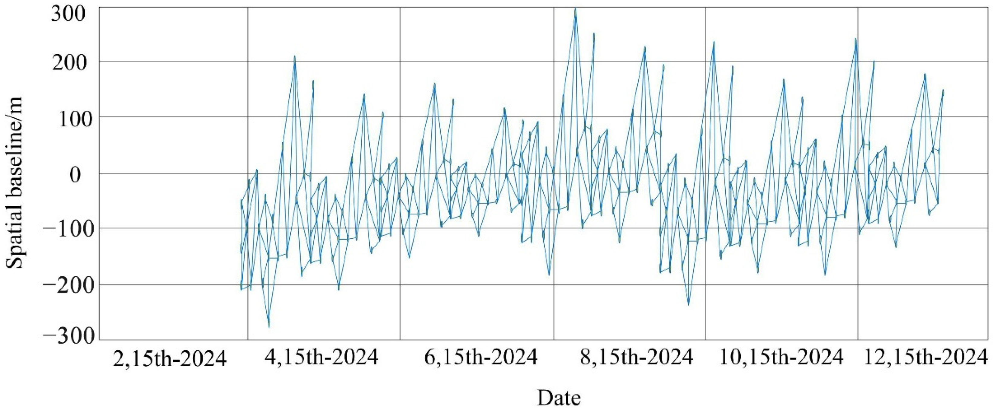
Among them, $\lambda$ represents the singular value decomposition coefficient; $L$ represents the matrix integral calculation coefficient. To ensure computational efficiency, the time threshold is set to 180, and the spatial threshold is set to 160. Due to the significant impact of spatiotemporal thresholds on interferograms, it is easy to cause a surge in noise. Therefore, the average dryness threshold of the interferogram is set to 0.5, and the spatiotemporal baseline map of the target landslide is shown in Figure 7. Due to the high precision requirements for deformation data and feature point data in landslide spatiotemporal analysis, Generic Atmospheric Correction Online Service (GACOS) data were used to eliminate atmospheric noise and further eliminate data errors in the process of drawing Figure 7. At the same time, setting the amplitude deviation of the curve to 0.3 and the standard deviation threshold to 0.5 further reduces the number of data points in the SBAS-InSAR image, improves the computational data, and ensures the reliability of the temporal curve.

4.2. Temporal and Spatial Analysis Results of Landslides

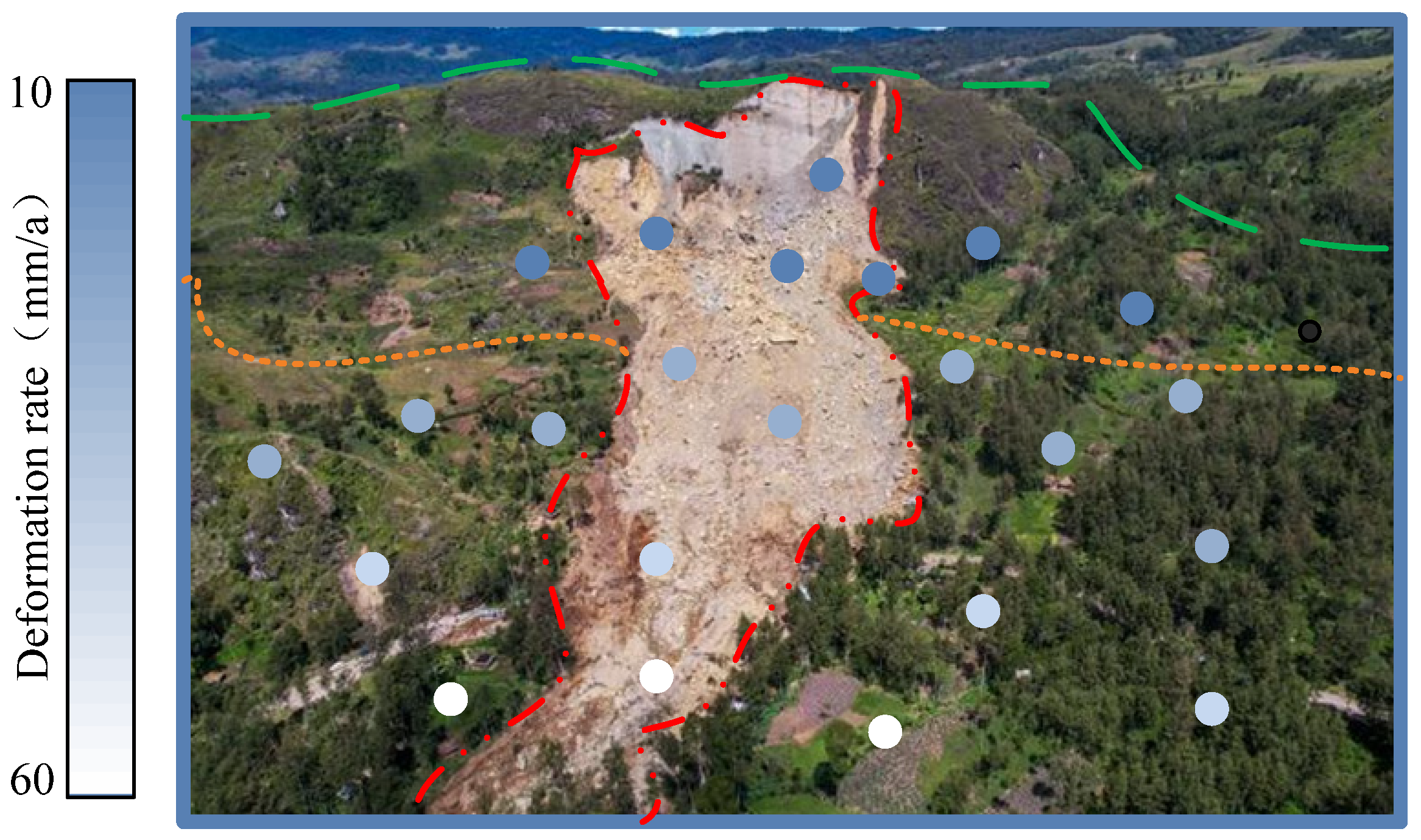
This study applied SBAS-InSAR technology to obtain satellite images of the research area, with data sourced from the Sentinel-1 satellite of the European Space Agency (ESA). This satellite provides C-band SAR data with wide coverage and a high revisit period, ensuring the continuity and reliability of data acquisition. Regarding the issue of time resolution, Sentinel-1 satellite has a revisit period of 6 days.

The image shown in Figure 8 was obtained using SBAS-InSAR technology.

By analyzing Figure 8, it can be seen that most of the landslides occur in the middle and lower parts of the landslide area in the image, and the overall deformation speed is controlled at 10~60 mm/a. Specifically, the strong deformation zone of the landslide is located in the middle and upper parts of the landslide body, which is the area of stress concentration and it is more prone to tensile and shear deformation. Due to the influence of friction and resistance, the deformation rate of the landslide bottom is relatively low, and it is more manifested as accumulation and sedimentation. Through analysis, it can be seen that the deformation velocity of the middle and lower squares in the landslide area is greater than that of the middle and upper squares in the landslide area, and the deformation velocity of the potential influence areas on both sides is greater. This deformation spatial differentiation phenomenon can be attributed to the stress transfer and energy release mechanism of the landslide body. The middle and lower sliding bodies have a high degree of shear stress concentration due to the presence of the leading-edge free surface, and the saturation degree of the sliding zone is directly affected by fluctuations in the reservoir’s water level, resulting in periodic loss of effective stress. The upper and middle sliding bodies are controlled by the tension cracks at the trailing edge, and the deformation is mainly characterized by tension creep, with a lower energy release rate. In addition, the two sides of the landslide are constrained by terrain, and the lateral frictional resistance limits the transmission of deformation, forming a mechanical pattern of “central drive lateral blockage”.

To verify the reliability of the spatiotemporal analysis results, the methods of reference [5], reference [6], and reference [7] were selected to conduct spatiotemporal analysis on the target landslide, and the application effects of different methods were determined through the following four sets of data.

To visually compare the data in

Table 2. Comparison table of results.

		RMES/mm	MAE/mm	Cosine Similarity	Accumulated Displacement Difference/mm
Monitoring point 1	method of this study	11.65	10.45	0.98	15.21
	method of reference [5]	12.65	13.54	0.95	14.51
	method of reference [6]	12.66	14.05	0.85	20.62
	method of reference [7]	12.95	14.98	0.94	21.44
Monitoring point 2	method of this study	15.01	11.24	0.99	16.20
	method of reference [5]	17.41	12.41	0.98	26.15
	method of reference [6]	17.55	14.05	0.98	25.22
	method of reference [7]	16.84	14.55	0.92	30.14
Monitoring point 3	method of this study	11.08	11.62	0.99	14.21
	method of reference [5]	12.41	10.66	0.95	25.41
	method of reference [6]	13.54	11.84	0.94	30.66
	method of reference [7]	13.66	11.95	0.90	31.85
Monitoring point 4	method of this study	11.51	11.54	0.99	15.20
	method of reference [5]	12.44	12.85	0.95	26.51
	method of reference [6]	13.06	16.95	0.84	24.15
	method of reference [7]	14.85	17.44	0.97	22.03

, it should be plotted as an image, as shown in Figure 9.

From the analysis of the data in Table 2 and Figure 9, it can be seen that there are significant differences in the calculation results of various indicators for the method of this study and other methods in the literature. The calculation results of the method of this study are superior to those of other methods. Although there are some errors in the spatiotemporal analysis results of the method of this study, it can, to some extent, reflect the spatiotemporal characteristics of landslide deformation. Based on the above analysis results, it can be concluded that the method of this study can effectively monitor the spatiotemporal characteristics of the target landslide, and the obtained spatiotemporal monitoring data have high accuracy and small errors. Therefore, the spatiotemporal analysis method set in the previous text has certain feasibility.

To further verify the reliability of deformation data obtained by SBAS-InSAR technology, this study cross-validated the InSAR results by combining data from fully automatic surface displacement sensors at four monitoring points.

Firstly, spatiotemporal matching between the deformation time series generated by SBAS-InSAR and the displacement data from monitoring point sensors is performed. The time resolution of SBAS-InSAR data is 12 days, while sensor data are continuously monitored (sampled daily). To eliminate time scale differences, the sensor data are smoothed with a mean of 12 days to align with the InSAR data time nodes. Spatially, a 100 m × 100 m InSAR pixel area around each monitoring point is selected, the average deformation rate within that area is calculated, and it is used as the InSAR deformation value for the corresponding monitoring point location.

Then, statistical indicators are used to evaluate the consistency between the two data sources, including:

(a)

Root Mean Square Error (RMSE): measures the absolute difference in deformation rate between two variables;

(b)

Pearson’s correlation coefficient (Pearson’s r): evaluates the linear correlation of deformation trends;

(c)

Mean Absolute Error (MAE): reflects the robustness of data bias.

In addition, a relationship model between sensor data and InSAR data was established through linear regression analysis to verify whether the slope is close to 1 and the intercept is approaching 0.

The analysis results of the four monitoring points show that:

(a)

The MSE range is 9.2–13.8 mm/a, indicating that the absolute error of the two datasets is within an acceptable range;

(b)

Pearson’s correlation coefficient ranges from 0.86 to 0.93, indicating a highly consistent deformation trend;

(c)

The slope of linear regression is 0.91–1.05, and the intercept is −2.1–1.8 mm/a, further confirming the linear matching between the data.

5. Analysis of the Instability Trend of the Step Deformation Landslide

In terms of landslide instability trend analysis, this study constructed a landslide prediction model and corrected the prediction error using an ELM neural network. The obtained prediction results were used as the data analysis source for the landslide deformation coefficient to determine the direction of landslide instability trend. ELM is a single-hidden-layer feedforward neural network with fast learning speed and good generalization ability. Landslide deformation data often have nonlinear characteristics, and ELM neural networks can effectively process such data and provide more accurate prediction results.

5.1. Prediction of Step Landslide

In response to the basic characteristics of step landslides, this study will first construct a landslide prediction model. This model is divided into two parts, and the specific operation settings are as follows:

Part 1: Preliminary Prediction.

A combined prediction module for complex geological information is built. Starting from the requirement of accuracy in prediction results, this study applies the expected weight method to determine the combination weights. The specific solution process can be expressed as follows:

$${\eta }^1(i)={\displaystyle \frac{(\frac{1}{U(i)})}{({\displaystyle \sum _{i=1}^n\frac{1}{U(k)}})}}$$

(15)

$${\eta }^2(i)={\displaystyle \frac{(\frac{1}{D(i)})}{({\displaystyle \sum _{i=1}^n\frac{1}{D(k)}})}}$$

(16)

Among them, ${\eta }^1(i)$ represents the expected weight; ${\eta }^2(i)$ represents the variance weight; $U(i)$ represents the expected value of the residual sequence; $D(i)$ represents the variance value of the residual sequence.

At the same time, considering the stability of the prediction model, the fitted expected weights are added to the variance to obtain the cumulative index of the regression model:

$$c(i)={\eta }^1(i)+{\eta }^2(i)$$

(17)

According to the formula above, it can be determined that the larger the value of $c(i)$, the parameter settings of the ELM neural network are as follows:

The number of hidden layer nodes is set to 100 to balance model complexity with overfitting and underfitting risks;

The Sigmoid function is selected as the activation function to effectively handle the nonlinear features in landslide deformation data;

The weight matrices of the input layer and hidden layer are randomly initialized and kept unchanged, with a dimension of 5 × 100;

The hidden layer threshold vector is also randomly initialized and kept unchanged, with a dimension of 100 × 1;

The dimension of the output layer weight matrix is 100 × 1 (the output data dimension is 1, which is the predicted variable), and the least squares method is used to ensure that the model converges quickly and achieves high prediction accuracy, thereby effectively correcting the errors in the preliminary prediction results, which are greater the combined weight of the model. Therefore, this formula is organized as the final combined weight $c’(i)$:

$$c’(i)={\displaystyle \frac{c(i)}{{\displaystyle \sum _{i=1}^{n}c(i)}}}$$

(18)

After the calculation of this formula is completed, the corresponding prediction results can be obtained. Nevertheless, there are some errors, and an error correction step needs to be designed to remove the erroneous data.

Part 2: Error Correction.

In this study, an ELM neural network [19,20] was used to modify the calculation results obtained from Formula (7).

Assuming that the obtained calculation sample is $(z_i,t{’}_i)$, which contains $n$ elements $z_i$, the learning machine with $Y$ hidden layer nodes is represented as follows using the excitation function $b(z)$:

$${\displaystyle \sum _{i=1}^Y{\partial }_i}b({\varphi }_i{z}_i+u_i)={\wp }_i$$

(19)

Among them, ${\partial }_i=({\partial }_{i1},{\partial }_{i2},\dots ,{\partial }_{in})$ represents the weight vector between the $i$-th hidden layer node and the output node; ${\varphi }_i=({\varphi }_{i1},{\varphi }_{i2},\dots ,{\varphi }_{in})$ represents the weight vector between the output node and the $i$-th hidden layer node; $u_i$ represents the target neuron threshold; ${\wp }_i=({\wp }_{i1},{\wp }_{i2},\dots ,{\wp }_{in})$ represents the output vector. The number of hidden nodes in an ELM directly affects the complexity of the model. If there are too many hidden layer nodes, the model may overfit the training data; if the number of hidden layer nodes is too small, it may lead to underfitting. Therefore, this study dynamically adjusts the number of hidden layer nodes based on the complexity of the training data, thereby further reducing the risk of overfitting.

According to the basic operating principle of a learning machine, it can approximate training samples with zero error, which includes:

$${\displaystyle \sum _{i=1}^Y‖{\wp }_i-t{’}_i‖}=0$$

(20)

According to this formula, ${\partial }_i$, ${\varphi }_i$, and $u_i$ should satisfy:

$${\displaystyle \sum _{i=1}^Y{\partial }_i}b({\varphi }_i{z}_i+u_i)=r_i$$

(21)

Among them, $r_i$ represents the expected value at the target node. To improve computational efficiency, the formulas above can be integrated into a matrix form, which includes:

$$P\partial =R$$

(22)

Among them, $P$ represents the data output matrix of the learning machine. This learning process can be expanded using the least squares solution, which includes:

$$\partial ’=P’R$$

(23)

Among them, $P’$ represents the generalized inverse matrix of matrix $P$. The formula above is used to correct the error in the results obtained from Formula (7) and verify the validity of the predicted results, which will serve as the basis for subsequent trend analysis.

5.2. Analysis of Deformation Trend of Step Landslide

This study divides the analysis of the deformation trend of step landslides into two parts, with the following specific settings:

(A)

Detection of the overall deformation coefficient of the landslide range

The deformation time series data within the landslide range are set as $X’=\left[X{’}_1,X{’}_2,\dots ,X{’}_n\right]$, and the above data columns are sorted according to the size of the deformation data to obtain the data column $Q’=\left[Q{’}_1,Q{’}_2,\dots ,Q{’}_n\right]$ again. Based on the above two data columns, the equal rank of the deformation sequence is obtained:

$$\omega =1-{\displaystyle \frac{6{\displaystyle \sum _{i=1}^N{(X{’}_i-X{’}_i)}^2}}{N^3-N}}$$

(24)

Among them, $\omega$ represents the rank of the evaluation sequence; $N$ represents the total number of data samples. Based on this calculation result, $\omega$ is used to determine the critical value $F’$ of the deformation coefficient and determine the overall deformation trend of the landslide range:

① If $\left|\omega \right|<F’$, this indicates that the calculation result obtained from Formula (24) has no practical significance and requires secondary calculation;

② If $\left|\omega \right|\ge F’$, this indicates that the results obtained from Formula (24) have analytical value and can be subjected to more detailed deformation trend analysis.

(B)

Analysis of landslide deformation trend

Based on the verification results above, assuming the null hypothesis, the preliminary statistical measure of deformation trend can be expressed as follows:

$$L’={\displaystyle \sum _{i=1}^{n-1}{\displaystyle \sum _{i=1+i}^n\mathrm{sgn}(Q{’}_j-Q{’}_i)}}$$

(25)

$$\mathrm{sgn}(\cdot )=\left\{\begin{array}{c}1, (\cdot )>0\hfill \\ 0, (\cdot )=0\hfill \\ -1, (\cdot )<0\hfill \end{array}\right.$$

(26)

Among them, $L’$ represents the preliminary statistical value of deformation data. Based on this statistical value, the final trend evaluation indicator $G’$ is obtained:

$$G’=\left\{\begin{array}{l}\begin{array}{cc}{\displaystyle \frac{L’-1}{\sqrt{\mathrm{var}(L’)}}}\hfill & L’>0\end{array}\\ \begin{array}{c}0 L’=0\hfill \end{array}\\ \begin{array}{cc}{\displaystyle \frac{L’+1}{\sqrt{\mathrm{var}(L’)}}}& L’<0\end{array}\end{array}\right.$$

(27)

Among them, $\mathrm{var}(L’)={\displaystyle \frac{[n(n-1)(2n+5)]}{n}}$. Based on the significance calculation results, the critical value $G{’}_{1-{\displaystyle \frac{n}{2}}}$ is validated and compared with $G’$, resulting in:

① When $G’>G{’}_{1-{\displaystyle \frac{n}{2}}}$, the deformation trend shows an upward trend;

② When $G’<G{’}_{1-{\displaystyle \frac{n}{2}}}$, the deformation trend shows a downward trend.

By organizing the above calculation content, it can be used to analyze the deformation trend of the target landslide.

5.3. Analysis Results of Landslide Deformation Trend

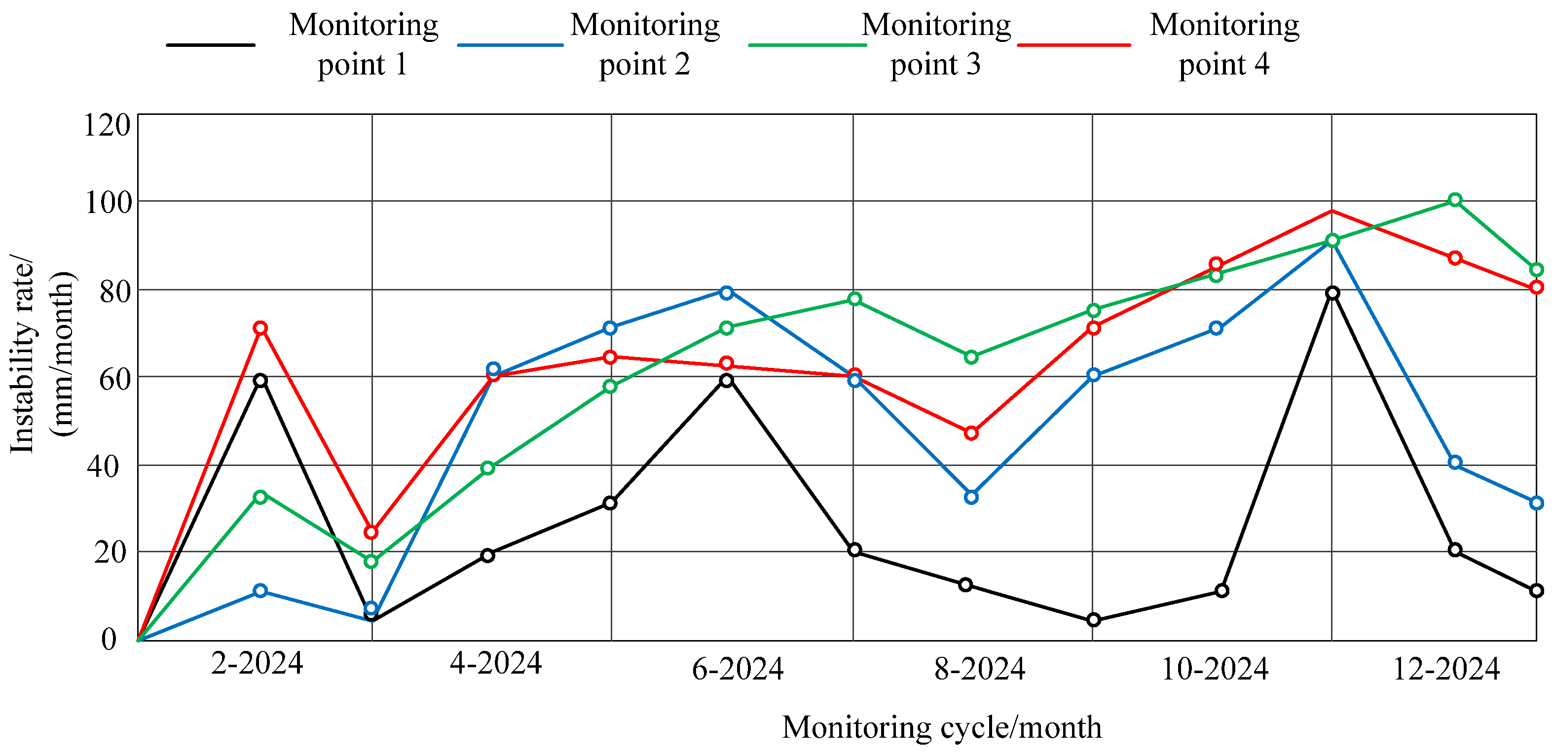
Using the content in Figure 5 as the basis for landslide deformation trend analysis, the landslide deformation rate curve is drawn, as shown in Figure 10.

Based on this curve, Matlab fitting software is used to make initial predictions on this deformation data and obtain the fitting prediction results. At the same time, using the calculation section set in the previous text, the difference between the predicted results and the monitoring results of the four measurement points is obtained. To ensure the accuracy of the test results, the 15th day data of each month during the test period are predicted and compared with the actual monitoring values. The specific results are shown in

Table 3. Comparison of landslide deformation prediction results.

Monitoring Month	Monitoring Point 1		Monitoring Point 2		Monitoring Point 3		Monitoring Point 4
	Monitoring Results/mm	Forecast Results /mm	Monitoring Results/mm	Forecast Results /mm	Monitoring Results/mm	Forecast Results /mm	Monitoring Results/mm	Forecast Results /mm
1	209.08	209.00	219.62	219.62	227.77	220.55	229.46	230.52
2	219.83	218.83	213.35	222.35	223.48	218.48	222.27	214.77
3	216.65	215.55	212.21	217.21	225.32	224.32	217.34	217.34
4	210.06	212.06	224.61	220.45	226.33	221.85	220.23	208.53
5	225.16	225.16	228.13	220.15	218.74	217.22	222.98	222.64
6	214.33	214.33	214.36	214.36	226.57	220.58	219.18	215.84
7	209.41	209.41	211.81	211.05	220.01	214.85	222.25	208.25
8	220.22	220.22	222.28	220.66	213.56	222.58	223.13	218.22
9	226.49	226.49	218.26	213.68	223.28	223.28	217.01	211.84
10	211.14	211.10	218.57	214.52	225.40	245.81	218.00	212.65
11	208.59	207.59	217.79	215.62	215.76	213.14	225.64	207.85
12	205.12	204.22	213.12	209.12	223.85	215.00	218.41	207.44

.

From the data in Table 3, it can be seen that the prediction model proposed in this study has practical value, with small errors between the predicted results and the actual monitoring data. The stability of the data obtained by the prediction model is high, and the prediction results of each monitoring point are relatively similar, which also confirms the high generalizability of the prediction model. According to the data in Table 3, it can be determined that during the monitoring period, the deformation of the landslide area gradually increases and maintains a continuous growth trend.

To further obtain the deformation trend of the landslide, the trend judgment process is completed using the predicted results obtained from Table 3. The data in Table 3 are substituted into Formulas (24)–(27), and the calculated results are shown in

Table 4. Analysis results of the landslide instability trend.

Monitoring Point	Original Data Column		Processed Data Column
	Verify the Calculation Results	Significance Level	Verify the Calculation Results	Significance Level
1	3.152	Very significant	3.095	Very significant
2	3.220	Very significant	3.152	Very significant
3	2.084	Very significant	2.055	Very significant
4	2.954	Significant	2.877	Significant

.

In this study, the test value for values above 99.0% was set as very significant, and the test value for values above 95.0% was set as significant. Based on this result, it can be determined that the deformation trend of the target landslide shows an increasing trend during the monitoring period, which is consistent with the predicted results in Table 3, confirming that the reliability of the trend prediction results is relatively high.

5.4. Trend Verification Based on Mechanical Instability Criteria

To further enhance the engineering applicability of instability trend analysis, this study combines the principles of geomechanics and introduces typical mechanical instability criteria to verify the predicted results. The instability essence of a step landslide is that the shear strength of the sliding zone soil is insufficient to resist shear stress, and its mechanical equilibrium can be expressed as follows:

$$F_s={\displaystyle \frac{{\tau }_f}{\tau }}={\displaystyle \frac{c’+\left({\sigma }_n-u\right)\tan \varphi }{\tau }}$$

(28)

In the formula, $F_s$ represents the safety factor; ${\tau }_f$ represents shear strength; $\tau$ represents the actual shear stress; $c’$ represents effective cohesion; ${\sigma }_n$ represents normal stress; $u$ represents pore water pressure; $\varphi$ represents the effective internal friction angle. When $F_s<1$, the landslide enters the stage of accelerated instability.

According to the double-layer structural characteristics of the target landslide, the upper pore water is rapidly discharged during the sudden drop in the reservoir’s water level, resulting in a sharp decrease in the effective normal stress $\left({\sigma }_n-u\right)$ of the sliding zone and a significant weakening of the shear strength.

A three-dimensional finite element model is established using Geostudio software to simulate the spatiotemporal evolution of $F_s$ under different water level decelerations. The results indicate that when the water level drops by more than 1.5 m/d, the $F_s$ at the leading edge of the slip zone drops below 0.95, which is highly consistent with the deformation acceleration zone monitored by InSAR, thus verifying the spatial consistency between the mechanical instability criterion and the deformation data.

6. Discussion

To confirm the practical value of the deformation trend analysis method proposed in this study, the trend of the target landslide was analyzed using methods of reference [5], method of reference [6], and the method of reference [7] in conjunction with the method of this study. The absolute error rates of different methods were obtained by comparing them with real data. The experimental results are shown in

Table 5. Error rate of unstable prediction data for measuring points (unit: %).

Monitoring Month	Method of This Study	Method of Reference [5]	Method of Reference [6]	Method of Reference [7]
1	1.02	3.49	3.75	6.64
2	1.39	5.29	4.89	5.58
3	1.39	2.05	5.49	6.04
4	1.49	4.02	5.33	6.45
5	1.11	3.02	4.19	5.88
6	1.05	2.57	4.73	4.41
7	1.42	4.04	4.21	7.01
8	1.02	4.92	3.64	7.04
9	1.24	3.32	5.09	6.32
10	1.16	4.38	5.09	4.19
11	1.42	3.56	2.38	4.01
12	1.08	2.63	4.24	5.31

. To reduce the difficulty of experimental calculations, the data from measurement point 3 were used as the data basis, and only the content of this measurement point is predicted.

Comparing the data in Table 5, it can be seen that for monitoring point 3, there is a certain degree of error in the predicted results of the method of this study compared to the other three methods. However, the error of this study method is relatively small and close to the measured results. Meanwhile, through comparison, it can also be seen that the method of this study has relatively small differences between each month in the monitoring period, indicating that the data are generally stable. Based on the above results, it can be determined that the method of this study has higher prediction accuracy and more reliable data. According to the calculation process set in the previous text, the landslide instability trend analysis results of the other three methods were calculated, and the results are shown in

Table 6. Analysis results of landslide instability trend (method of reference [5]).

Monitoring Point	Original Data Column		Processed Data Column
	Verify the Calculation Results	Significance Level	Verify the Calculation Results	Significance Level
1	3.150	Very significant	3.080	Very significant
2	3.220	Significant	3.152	Significant
3	2.084	Significant	2.055	Significant
4	2.015	Not significant	2.143	Not significant

,

Table 7. Analysis results of landslide instability trend (method of reference [6]).

Monitoring Point	Original Data Column		Processed Data Column
	Verify the Calculation Results	Significance Level	Verify the Calculation Results	Significance Level
1	3.014	Very significant	2.981	Very significant
2	1.154	Not significant	1.024	Not significant
3	2.415	Significant	2.117	Significant
4	2.015	Not significant	2.143	Not significant

and

Table 8. Analysis results of landslide instability trend (method of reference [7]).

Monitoring Point	Original Data Column		Processed Data Column
	Verify the Calculation Results	Significance Level	Verify the Calculation Results	Significance Level
1	3.152	Very significant	3.095	Very significant
2	3.220	Very significant	3.152	Very significant
3	1.158	Not significant	1.021	Not significant
4	2.744	Significant	2.671	Significant

.

From the analysis of the above data, it can be seen that although the three methods mentioned above can also predict the instability of step deformation landslides, the results obtained from the method of reference [5] confirm that the deformation trend of landslides shows a downward trend; the results obtained from the method of reference [6] confirm that the deformation trend of the landslide presents a stable state; the results obtained from the method of reference [7] confirm that the deformation trend of landslides shows a slow upward trend. The instability trend prediction results obtained by the three methods above have significant differences from actual monitoring, indicating that these three methods still need to be optimized separately. Based on the above experimental results, it can be determined that the landslide instability trend analysis results of the method of this study are more reliable.

In summary, in this study, step deformation landslides were selected as the research object, and the following results were obtained:

① A step deformation landslide has high spatiotemporal characteristics, and the deformation velocity of the middle lower square in the landslide area is greater than that of the middle upper square in the landslide area, and the deformation velocity of the potential influence areas on both sides is greater. On an annual basis, the step deformation is concentrated in March and April, the landslide deceleration is concentrated in May and June, and the landslide acceleration is concentrated in July and August. The stability time throughout the year is relatively short.

② The spatiotemporal analysis method and instability trend analysis method proposed in this article are superior to traditional methods. In subsequent research, this study method can be used as the main research technique for step deformation landslides. This is because the method of this study combines advanced SBAS-InSAR technology and an ELM neural network for error correction. SBAS-InSAR technology effectively reduces the impact of atmospheric delay and terrain errors by selecting a small subset of baselines, providing higher precision deformation measurement data, and making landslide deformation spatiotemporal analysis more accurate. Meanwhile, the application of an ELM neural network significantly improves the stability and accuracy of the prediction model, and can more accurately capture the nonlinear characteristics of landslide deformation. Compared with traditional methods, the method of this study performs well in handling complex terrain, dealing with nonlinear deformation, and improving prediction accuracy. Therefore, it can better analyze the instability trend of landslides and provide a more reliable scientific basis for the prevention and control of landslide disasters.

7. Conclusions

This study conducted an in-depth exploration of the deformation spatiotemporal analysis and instability trend analysis of step deformation landslides.

Firstly, the geological characteristics, precipitation data, and historical displacement records of the target landslide area were systematically analyzed. Using the slope single-change-point analysis method, the characteristic points of the monitoring data were successfully extracted, laying a robust foundation for a subsequent analysis. SBAS-InSAR technology was then employed to obtain satellite images of the study area. By integrating the extracted feature points, the spatiotemporal baseline of the target landslide was drawn, and detailed spatiotemporal analysis was completed. During this process, the small baseline subset selection strategy of SBAS-InSAR effectively minimized the impact of atmospheric delays and terrain errors, delivering high-precision deformation measurement data. This highlighted its unique advantages in landslide monitoring in complex terrain areas.

For landslide instability trend analysis, a prediction model was constructed, and the ELM neural network was innovatively applied to correct prediction errors. This significantly enhanced the accuracy and stability of prediction results. The research findings revealed that step deformation landslides exhibit pronounced spatiotemporal characteristics, with a relatively short stability time throughout the year. Landslide deformation is mainly concentrated within specific time intervals, with square deformation velocity in the middle and lower parts of the landslide area being significantly higher than that in the middle and upper parts, and there being adjacent potential impact areas on both sides.

A comparison with existing methods showed that the spatiotemporal analysis method and instability trend analysis method proposed in this study exhibit better performance. Specifically, in deformation spatiotemporal analysis, the RMES MAE, cosine similarity, and cumulative displacement difference indicators exhibited superior performance, reflecting higher monitoring accuracy and reliability. In terms of instability trend analysis, the prediction error rate of this study method was significantly lower than that of existing methods, with the prediction outcomes highly consistent with the measured data, confirming their effectiveness in practical applications.

In summary, this study not only deepens the understanding of the deformation mechanism of step deformation landslides but also provides more scientific and reliable methodologies for the prevention and control of landslide disasters. Future research will focus on further optimizing and improving these methods, as well as expanding the scope of research, to achieve more groundbreaking results in landslide monitoring and early warning. We will strive to introduce additional data sources, such as more detailed hydrological data (including changes in reservoir water levels, groundwater dynamics, etc.) and seismic activity data, to more comprehensively capture the multi-physics field coupling effects of landslide deformation. Secondly, we will explore and apply alternative machine learning algorithms, such as Convolutional Neural Networks (CNNs) or Recurrent Neural Networks (RNNs) in deep learning, to further improve the accuracy and generalization ability of landslide prediction models. These enhanced features will guide our subsequent research work, with the aim of achieving more breakthrough results in the field of landslide monitoring and early warning.