Hydraulic Disconnection Between Aquifers: Assessing the Hydrogeologic Controls on Inter-Aquifer Exchange and Induced Recharge in Pumped, Multi-Aquifer Systems

Abstract

Unprecedented, long-term pumping is occurring in aquifers worldwide, necessitating a greater understanding of the impacts from significant water table drawdown. Drawdown-induced hydraulic disconnection can significantly alter rates of inter-aquifer exchange and recharge, yet it remains an understudied phenomenon in multi-aquifer systems. This study investigates the potential for drawdown-induced hydraulic disconnection and its impact on inter-aquifer fluxes between a perennially recharged alluvial aquifer and a heavily pumped bedrock aquifer. We employed three-dimensional, transient, variably saturated flow modeling, incorporating multiple realizations of varying sandstone channel fraction (20–75%), to simulate evolving saturation patterns and alluvium-to-bedrock (A-B) flow rates. The results demonstrate the initiation and propagation of inter-aquifer unsaturated zones within sandstone channels underlying thinner low-permeability mudstones, leading to a substantial reduction in A-B flow, with the normalized flow response function (ABRF) decreasing by up to 98%. Complex saturation patterns, dictated by sandstone–mudstone heterogeneity, emerged as controls for water table elevation, disconnection status, and flow pathways. Multiple linear regression (R² up to 0.88) identified the bedrock aquifer sandstone fraction and the vertical span of saturated, connected channels as significant predictors of maximum A-B flow. Substantial variability in maximum A-B flow rates across scenarios with identical sandstone fractions (coefficient of variation 0.17 to 0.29) demonstrates the impact of geologic heterogeneity and saturation state on inter-aquifer exchange rates. The results of this study illustrate that hydraulic disconnection is not limited to near-surface environments and that geologic heterogeneity is a key factor controlling inter-aquifer fluxes in heavily pumped multi-aquifer systems.

1. Introduction

Substantial groundwater pumping may result in disconnection between an aquifer and a surface water body or between two aquifers. Hydraulic disconnection refers to the situation where hydraulic heads along the boundary of a saturated water source are unaffected by pumping (or other source/sink stresses) within a deeper aquifer. Disconnection generally requires a significant unsaturated zone, and the critical hydrologic consequence is that recharge contributions from the shallow water source (i.e., surface water feature or perched aquifer) are not influenced by further water table decline in the deeper aquifer.

Disconnection dynamics have been extensively studied in the context of groundwater–surface water exchange [1,2,3,4,5]. When pumping lowers a water table beneath a surface water body, the presence of a low-hydraulic conductivity (low-K) unit (i.e., clogging layer) can initiate negative pressure in the underlying aquifer (high-K), causing air to enter the system. This unsaturated zone marks the onset of unsaturated flow, signaling a “transitional” flow regime wherein the decreasing saturation-dependent aquifer hydraulic conductivity and a rising hydraulic gradient increasingly drive flow through the low-K unit. Eventually, the flux asymptotically approaches a maximum value, implying a “disconnected” flow regime where further lowering of the water table no longer significantly affects the flux. Both transitional and disconnected regimes curtail the rate and timing of induced recharge compared to fully saturated systems [2]. Reductions in vertical recharge occur due to lowered effective hydraulic conductivity [3] and elongated and deflected flow paths imposed by the low-K connectivity structure [4,5]. As induced recharge becomes less available, pumped water is increasingly derived from alternative sources like aquifer storage [6]. As a result, systems that undergo pumping induced transition or disconnection may exhibit intensified head declines and storage loss, particularly where model predictions neglect to account for this process [7].

Because disconnection is exceedingly difficult to identify in the field, modeling is an essential tool for investigating and predicting disconnection. Through modeling, authors have identified geologic heterogeneity, or the distribution of low- and high-permeability subsurface materials, as a key controlling parameter for disconnection dynamics. Low-permeability units dictate if and where desaturation will initiate [2,8], while high-permeability units serve to provide preferential flow paths that dominate recharge [9,10], river seepage [8,11], and well pumping response [12,13,14,15,16]. Sharp hydraulic conductivity contrasts can further alter flow paths as low-conductivity units drive lateral flow, thereby reducing vertical fluxes and leading to thicker perched zones [4,5]. Spatial variations in connection status are directly attributed to patterns in subsurface heterogeneity [8,11,17]. Geometry, connectivity, and other properties of the heterogeneity structure are therefore critical considerations when studying disconnection dynamics, e.g., [8,18,19]. Unfortunately, incorporating detailed heterogeneity and unsaturated flow processes in regional models is often unfeasible due to computational demands.

While hydraulic disconnection has been considered for shallow regions beneath streams, lakes, and wetlands, e.g., [20,21,22,23], further research is needed to evaluate conditions that may lead to disconnection between aquifers in multi-aquifer systems. Unprecedented pumping in recent decades has led to groundwater depletion and extensive drawdown (>290 m) in heavily pumped aquifers around the world [24,25]. As groundwater is increasingly used to meet global water demands, the potential for disconnection may expand in these heavily pumped systems where it has not previously been documented.

This study provides a physics-based investigation of inter-aquifer hydraulic disconnection using variably saturated flow models parameterized with realistic geologic heterogeneity. Models are designed to represent conditions found in the heavily pumped Denver Basin, a crucial water resource for Colorado’s Front Range Urban Corridor. This multi-aquifer system includes bedrock aquifers comprising Late Cretaceous to Paleogene fluvial sandstones and mudstones, and they are overlain and incised by Quaternary Alluvial deposits that follow modern-day tributaries of the South Platte River. While streams and alluvial aquifers are replenished annually from mountain headwaters, bedrock aquifers receive limited recharge due to minimal outcrop extent and precipitation. This lack of deeper recharge coupled with long-term pumping has led to substantial groundwater depletion, lowering the bedrock aquifer water table by more than 80 m over the past century, and placing bedrock water tables well below the alluvium [26,27,28]. Regional models predict further declines and increased alluvial-to-bedrock flow [26], though they lack the resolution to capture the influence of detailed geologic heterogeneity (i.e., sandstone channel structure) within the bedrock aquifer that directly underlies the alluvial aquifer and saturation effects, which this study aims to address. Initial modeling identified the potential for induced hydraulic disconnection between the two aquifers, with geologic heterogeneity identified as a key controlling factor [28], though these efforts were limited to two dimensions and steady-state simulations.

In this study, we expand on previous work to investigate the potential for disconnection under 3D heterogeneous and transient conditions. We apply geostatistical methods that reproduce realistic aquifer heterogeneity and allow for multiple realizations along with variably saturated numerical flow models to simulate flow and saturation within the system. Specifically, we perform this work to evaluate how heterogeneity and saturation impact inter-aquifer exchange rates and flow paths that make up recharge to the deeper aquifer. Simulation results are analyzed to determine the controls on inter-aquifer exchange and hydraulic disconnection.

2. Materials and Methods

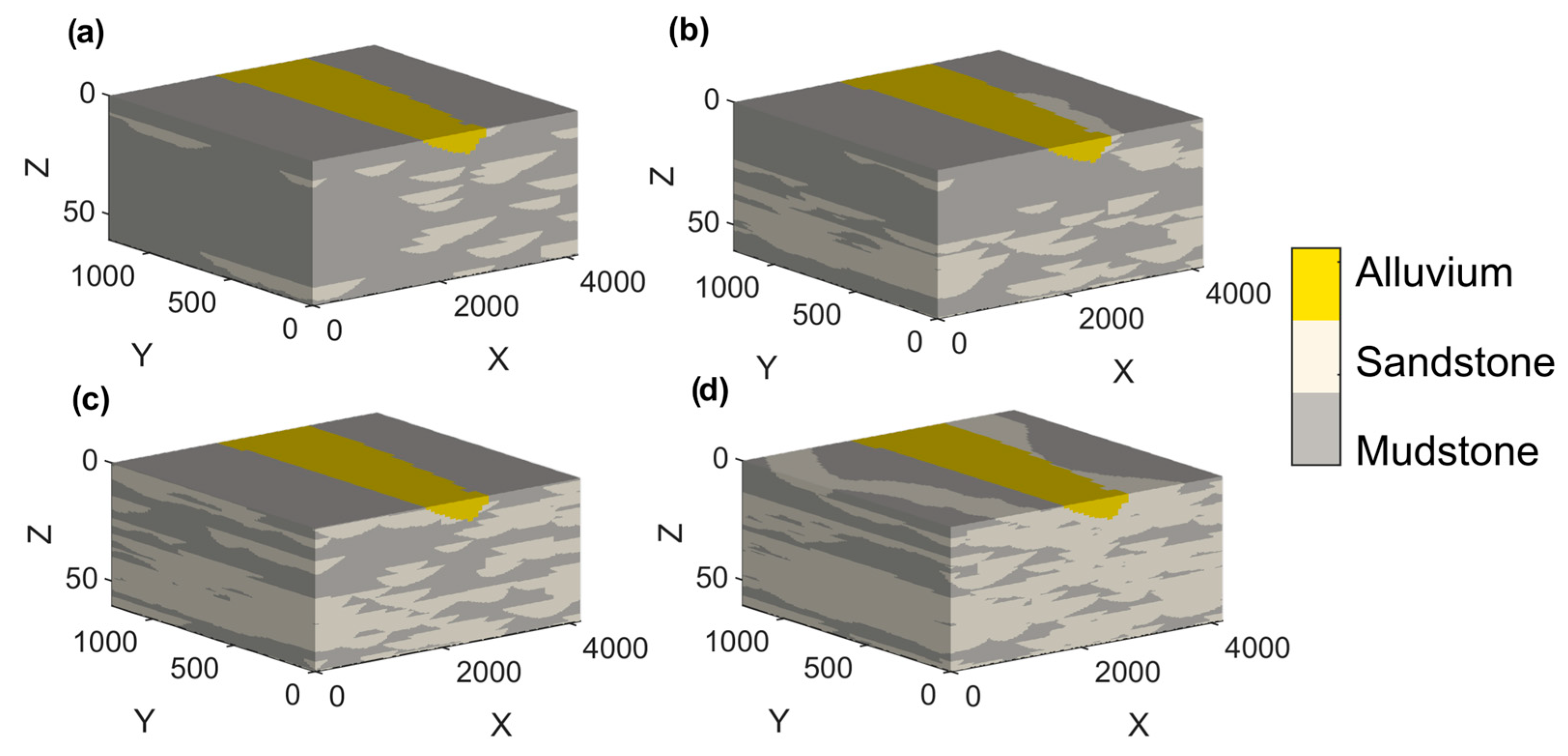
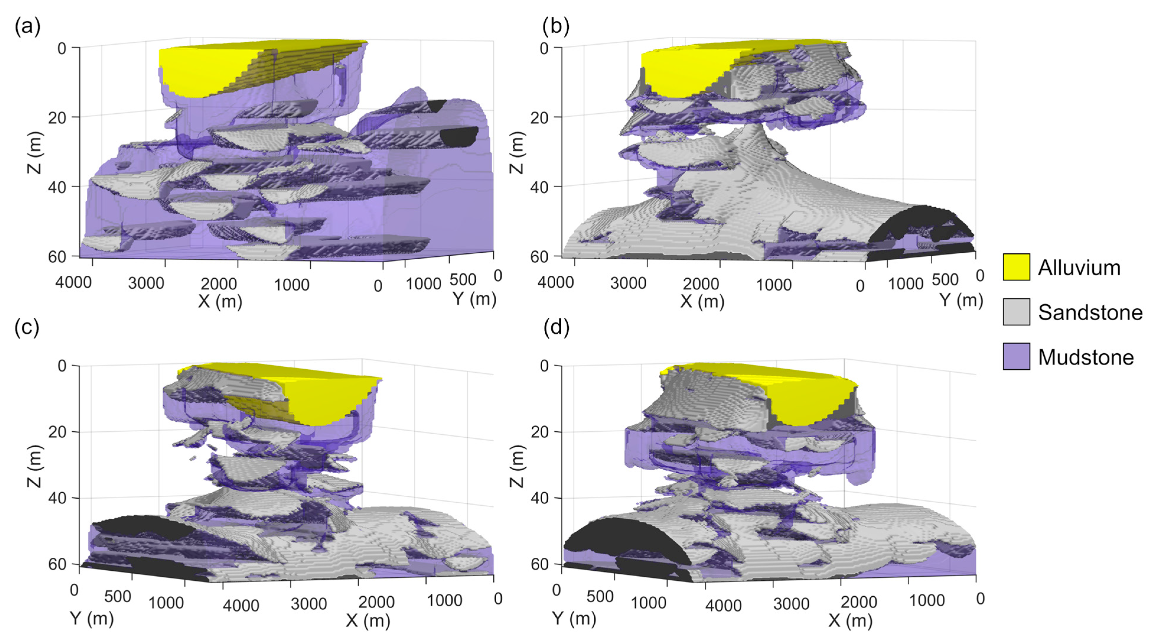
2.1. Geostatistical Simulation of Aquifer Heterogeneity

For variably saturated flow problems, the choice of geostatistical methods can strongly impact flow results, even across methods that enforce the same mean and variance [11]. Fluvial aquifers require methods that reproduce long-range connectivity of high-K units (i.e., channels) and low-K barriers to flow [29,30]. This study employed the object-based geostatistical modeling code FLUVSIM [31], which was specifically designed for fluvial settings. The algorithm successively places channel objects within a background overbank mudstone facies while allowing for conditioning to facies (i.e., borehole data) and geometry (i.e., channel fractions and dimensions).

Geostatistical simulations were constrained using lithofacies data from seven geophysical logs from an area in the south-central Denver Basin where significant bedrock aquifer pumping has occurred (central coordinates: 39.52851, −104.7837). Nearby wells screened in the uppermost bedrock aquifer show rates of water level decline that average −1 m per year⁻¹ (Figure S1 in Supporting Information). The upper geologic strata include coarse, multi-storied channel sandstone beds separated by overbank mudstones with trough-crossbedding [32]. Sandstone channels are, on average, 3–4 m thick and comprise approximately 30–40% of the strata. Lithofacies are relatively uniform with limited lateral compositional and textural variability. Detailed geophysical log locations and types are provided in the Supporting Information (Table S1 and Figures S2–S5).

Facies realizations were generated for a base case sandstone (channel) fraction of 35% and broader range fractions (20%, 50%, and 75%) to evaluate the influence of sandstone fraction on saturation and flow (Figure 1). Except for the 20% set, geostatistical simulations were conditioned to lithofacies from geophysical logs (i.e., sandstone or mudstone) in the study area, with maximum priority assigned to conditioning during channel placement. To avoid compromising channel proportion accuracy, conditioning was turned off for the 20% simulations. FLUVSIM’s input parameters, including model discretization and channel geometry information, are summarized in

Table 1. Geostatistical and variably saturated flow modeling input parameters.

FLUVSIM Parameters	Values
# rows, columns, layers	75, 152, 149
Δx, Δy, Δz	27.7 m, 16.9 m, 0.41 m
channel
proportions	20%, 35%, 50%, 70%
orientation	0° (North/South)
sinuosity (departure, length scale)	Departure 350 m; Length scale: 900 m
thickness	4 m ± 1 m
width-to-thickness ratio	200
MODFLOW-USG Parameters	Sandstone	Mudstone	Alluvium
Saturated Hydraulic Conductivity (m day−1)	0.3	0.001	65
Specific Storage (m−1)	0.000017	0.000056	0.0001
Specific Yield (-)	0.18	0.15	0.36
Specific Retention (-)	0.12	0.23	0.1
van Genuchten α (m−1)	0.79	1.9	14.5
van Genuchten n (-)	10.4	1.31	2.68
Brooks-Corey P (-)	3.21	9.45	4.19

.

The alluvial aquifer was represented as a single large channel with geometry constrained by bedrock depths from boring logs. Alluvial aquifer geometry was consistent across all geostatistical realizations (Figure 1).

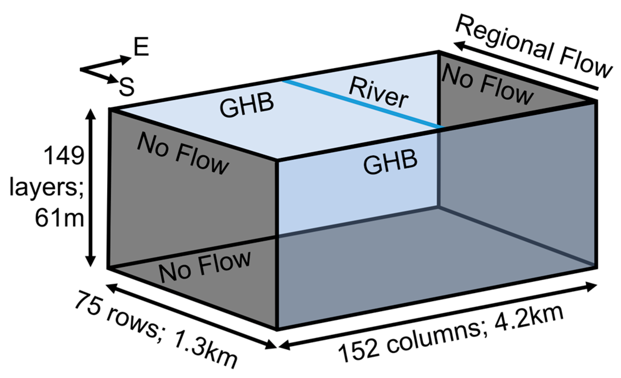
2.2. Variably Saturated Flow Modeling

Three-dimensional, variably saturated flow (VSF) modeling was performed to evaluate the impact of regional, long-term drawdown in the bedrock aquifer on fluxes and saturation throughout the stream–alluvial–bedrock system. Simulations were performed using the block-centered transport process for MODFLOW-USG vers. 1 (MFUSG), a finite-volume, unstructured grid version of MODFLOW that is able to simulate three-dimensional variably saturated subsurface flow [33,34] and has been applied to study similar issues [35,36]. MFUSG applies a control volume finite difference scheme to approximate a solution to the governing equation for 3D variably saturated transient flow [37]:

$${\displaystyle \frac{\partial }{\partial x}}\left(K_x{k}_{rw}{\displaystyle \frac{\partial h}{\partial x}}\right)+{\displaystyle \frac{\partial }{\partial y}}\left(K_y{k}_{rw}{\displaystyle \frac{\partial h}{\partial y}}\right)+{\displaystyle \frac{\partial }{\partial z}}\left(K_z{k}_{rw}{\displaystyle \frac{\partial h}{\partial z}}\right)-W=\varnothing {\displaystyle \frac{\partial S_w}{\partial t}}+S_w{S}_s{\displaystyle \frac{\partial h}{\partial t}}$$

(1)

where K_x, K_y, and K_z are the principal components of saturated hydraulic conductivity [L T⁻¹] along the x, y, and z axes, respectively; k_rw is the relative permeability, a dimensionless value that ranges from 0 to 1 as a function of water saturation; h is the hydraulic head [L]; W is a volumetric source or sink per unit volume [T⁻¹]; ∅ is the drainable porosity taken to be the specific yield (S_y); S_w is the degree of water saturation, which is a function of pressure head (ψ); S_s is specific storage [L⁻¹]; and t is time [T].

Functional expressions are used to relate the relative permeability, hydraulic head, and water saturation in the solution to Equation (1). Effective saturation, S_e, defined as (S_w – S_wr)/(1 – S_wr), where S_wr is the residual saturation, is calculated in MFUSG as a function of the pressure head through a modified van Genuchten equation [38]:

$$S_e={\displaystyle \genfrac{}{}{0pt}{}{{\left[1+{\left(\alpha \mathsf{\psi }\right)}^n\right]}^{-m} for \mathsf{\psi }<0}{1 for \mathsf{\psi }>0}}$$

(2)

where α, n, and m (m = 1 – 1/n) are the van Genuchten parameters, ψ is the pressure head [L] (ψ = h – z), and z is elevation. The relative permeability term (k_rw) utilized in Equation (1) is dependent on effective saturation, k_rw = S_e^P, with P being the Brooks-Corey coefficient [39].

The 3D model domain includes a stream–alluvial–bedrock aquifer sequence spanning 4686 m in the x-direction (east–west), 1260 m in the y-direction (north–south), and 70 m vertically below the streambed. The location and spatial extent were determined based on observed water level drawdown at monitoring wells and the availability of geophysical log data (Supporting Information Figure S2). Boundaries are oriented parallel to the direction of the stream and regional groundwater flow, which is towards the north. The domain is divided into a regularly spaced grid with 75 rows, 152 columns, and 149 layers with corresponding grid spacing of 27.7 m, 16.9 m, and 0.41 m in the x-, y-, and z-directions, respectively. Horizontal grid dimensions were selected to adequately represent channel geometry, and vertical spacing was set to the optimal spacing that produced stable flow results and minimized computation time.

The lateral and bottom edges of the model (x = 0, x = 4686, and z = 0 m) were assigned no-flow boundaries to reflect regional streamlines that run parallel to model edges (Figure 2). An assumption is made that minimal directional changes or cross gradients occur near these boundaries during flow simulations. The up- and down-gradient edges of the model (y = 0 and y = 1260) represent regional groundwater head contours for the alluvial and bedrock aquifers wherein the alluvial heads are relatively stable through time and the bedrock regional water table lowers from pumping wells beyond the extent of the model domain. These boundaries were assigned using no-flow boundaries and head-dependent flux boundaries as implemented with the General Head Boundary (GHB) Package of MODFLOW-USG vers. 1 [40]. The simulated flux into or out of GHB cells is proportional to the difference between a specified head value located outside the domain and the head calculated at the model boundary. External head values for alluvial aquifer GHB cells were constant through time. External heads for the bedrock aquifer were successively lowered during transient simulations at a rate of 1 m per year, which approximates the long-term rate of groundwater level decline recorded in nearby wells [41] (Supporting Information Figure S1). GHB conductance values were calculated using the hydraulic conductivity assigned to each cell. The perennial stream was modeled using a head-dependent flux boundary, as implemented in the River Package of MODFLOW-USG vers. 1 [40]. The simulated flux into or out of river cells is proportional to an assigned stream width, stage, and streambed hydraulic conductivity, as well as the calculated head difference between the stream and adjacent aquifer.

Aquifer hydraulic properties were assigned constant values for each simulated lithofacies (Table 1). K_x,y,z, S_s, and S_y were assigned based on published values for sandstone and mudstone units of D2 sediments [26,42,43,44]. The water retention parameters (S_wr, α, and n) for the alluvium are averages for sand samples reported by Carsel and Parrish [45], and those for the bedrock aquifer were assigned based on published estimates for similar sedimentary rocks [38,41,46]. Brooks-Corey coefficients were estimated from van Genuchten parameters using equivalence relationships developed by Seytoux et al. [47].

A flow simulation consisting of one steady state and 14 transient stress periods was performed for each of the 200 heterogeneity scenarios. Transient stress periods each spanned 5 years for a total simulation length of 70 years. Timestep lengths were automatically selected through an adaptive time-stepping algorithm and were allowed to vary between 0.1 and 200 days. Following each simulation, flow from the alluvial to bedrock aquifer was computed using the USGS program ZoneBudget-USG [48]. Unique zones were assigned to each lithofacies to calculate flow between units. Upgradient (1–5) and downgradient (71–75) rows were excluded from the analysis to avoid boundary effects.

Changes in modeled alluvial to bedrock flow due to water table lowering were documented with the percentage change in flow rate between stress periods (sp):

$$∆\{\mathrm{A-B} Flow\}=\left\{100\times \left(Q_{{AB}_{sp}}-Q_{{AB}_{sp-1}}\right)/Q_{{AB}_{sp-1}}\right\}$$

(3)

We also define a normalized A-B flow response function (ABRF) to directly quantify the relationship between bedrock water table change and flow response:

$$ABRF={\displaystyle \frac{{\left({∆Q}_{AB}/∆h\right)}^{sp} }{{\left({∆Q}_{AB}/∆h\right)}^1}}$$

(4)

where (ΔQ_AB/Δh)^sp is the change in A-B flow divided by the change in regional water table between successive stress periods (sp and sp-1), and (ΔQ_AB /Δh)¹ is the same ratio for the first transient stress period. For consistency, the final time step at the end of each stress period is used in calculations. ABRF is dimensionless, allowing for comparison across simulations with varying flow magnitudes. ABRF approaches zero for a disconnected flow regime, indicating no further increase in A-B flow with water table lowering.

2.3. Connectivity Metrics

The influence of sandstone channel connectivity on flow and saturation was evaluated using connectivity metrics. Static connectivity, describing the connectivity structure of a given parameter field as determined by the geologic architecture [18,49], was considered for high-K materials (sandstone and alluvium) using binary parameter fields where sandstone and alluvium were assigned a value of 1, and mudstone cells were assigned a value of 0. To account for the influence of changing saturation on connectivity, we also considered a saturation-dependent connectivity field by applying a threshold to the saturation-dependent hydraulic conductivity field in the final model timestep. Model cells with K(ψ) > 0.01 m day⁻¹ were assigned a value of 1, and all other cells were assigned a value of 0. The corresponding binary field and connectivity metrics are labeled as “dynamic”.

Connected component analysis was performed for each of the 200 simulated static and dynamic binary fields using the CONNEC3D program [50]. Each connected component (CC) is a unique body of connected high-K cells wherein cells are considered connected if they intersect along a 3D grid face [18]. Connectivity metrics used to summarize key aspects of the CC geometry include the total number of connected components (NCC), maximum number of cells for all CCs (MCC), the maximum vertical span (Z-dimension) for all CCs (ZCC), and the maximum vertical span for CCs that directly contact the alluvium (ABZCC). Saturation-dependent or dynamic conductivity statistics are indicated with “DY” appended to the variable name (i.e., NCC_DY, MCC_DY, ZCC_DY, and ABZCC_DY). The alluvium is expected to be more hydraulicly connected to the bedrock aquifer where channelized sandstones are in direct contact with alluvium. Connectivity at the alluvial–bedrock aquifer interface was quantified as the percentage of bedrock aquifer cells that share a face with alluvial aquifer cells and which contain sandstone, designated as A-B_{SS_%}.

Connectivity metrics were compared to the final (late-time) A-B flow rate for each simulation, and multiple linear regression analysis was performed to quantify whether and which connectivity metrics were the best predictors of variations in inter-aquifer exchange rates and hydraulic disconnection potential.

3. Results

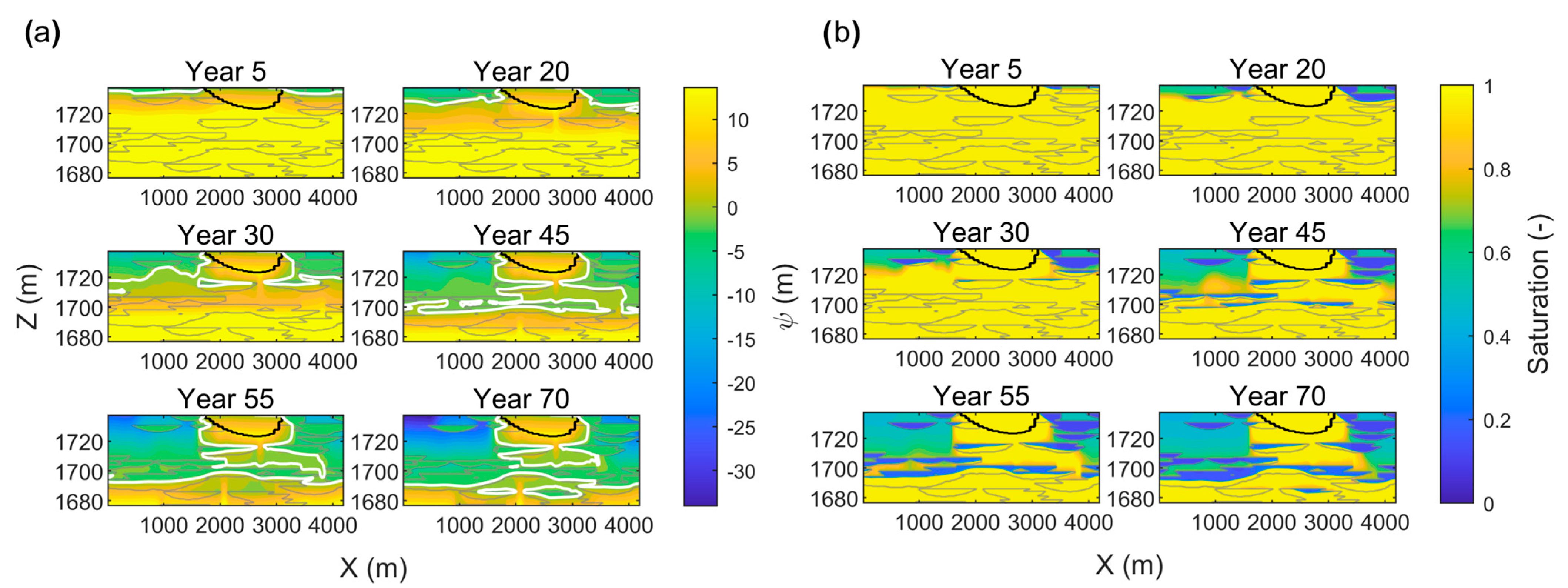
3.1. Pressure, Saturation, and Flux Dynamics

The VSF model was used to evaluate the effects of a declining bedrock water table on hydraulic heads, saturation, and inter-aquifer flow rates within the stream–alluvial–bedrock sequence. The simulation results from a representative scenario demonstrate the progression of modeled pressure heads (ψ) and saturation as the regional water table is lowered (Figure 3). Each panel corresponds to a simulation timestep wherein the year is equal to the magnitude of water table lowering in meters (i.e., rate = −1 m year⁻¹). The depth of the alluvium varies across the y-axis and is 14 m below the model top in the example cross-sectional slice.

At simulation year 5 (regional water table at 5 m below the model top), a continuous water table spans the alluvial and bedrock aquifers (i.e., ψ = 0 contour), with the bedrock aquifer pressure head increasing with depth (Figure 3a). By year 20 (water table 6 m below alluvium base), a low-pressure zone emerges beneath the alluvium, indicated by a low pressure head surrounding the uppermost sandstone channels. Year 30 (water table 16 m below alluvium) marks the onset of negative pressure (ψ < 0) beneath the alluvium, initiating unsaturated flow and a transitional flow regime. Notably, negative pressure begins in upper sandstone channels beneath outer margins of the alluvium (Figure 3a). Years 45, 55, and 70 (corresponding to water tables 31, 41, and 56 m below the alluvium base) show an expansion in the unsaturated zone between the alluvium and deeper water table (Figure 3a,b). The pressure head and saturation patterns reveal percolation features that connect saturated zones where flow occurs through saturated mudstone between unsaturated channels. By the final timestep, a perched alluvial aquifer is separated from the deeper water table by a partially to fully unsaturated zone. Saturation patterns remain irregular, reflecting fluvial architecture, with some connected channels becoming partially unsaturated in the upper channel, while the lower channel remains saturated, serving as conductive pathways.

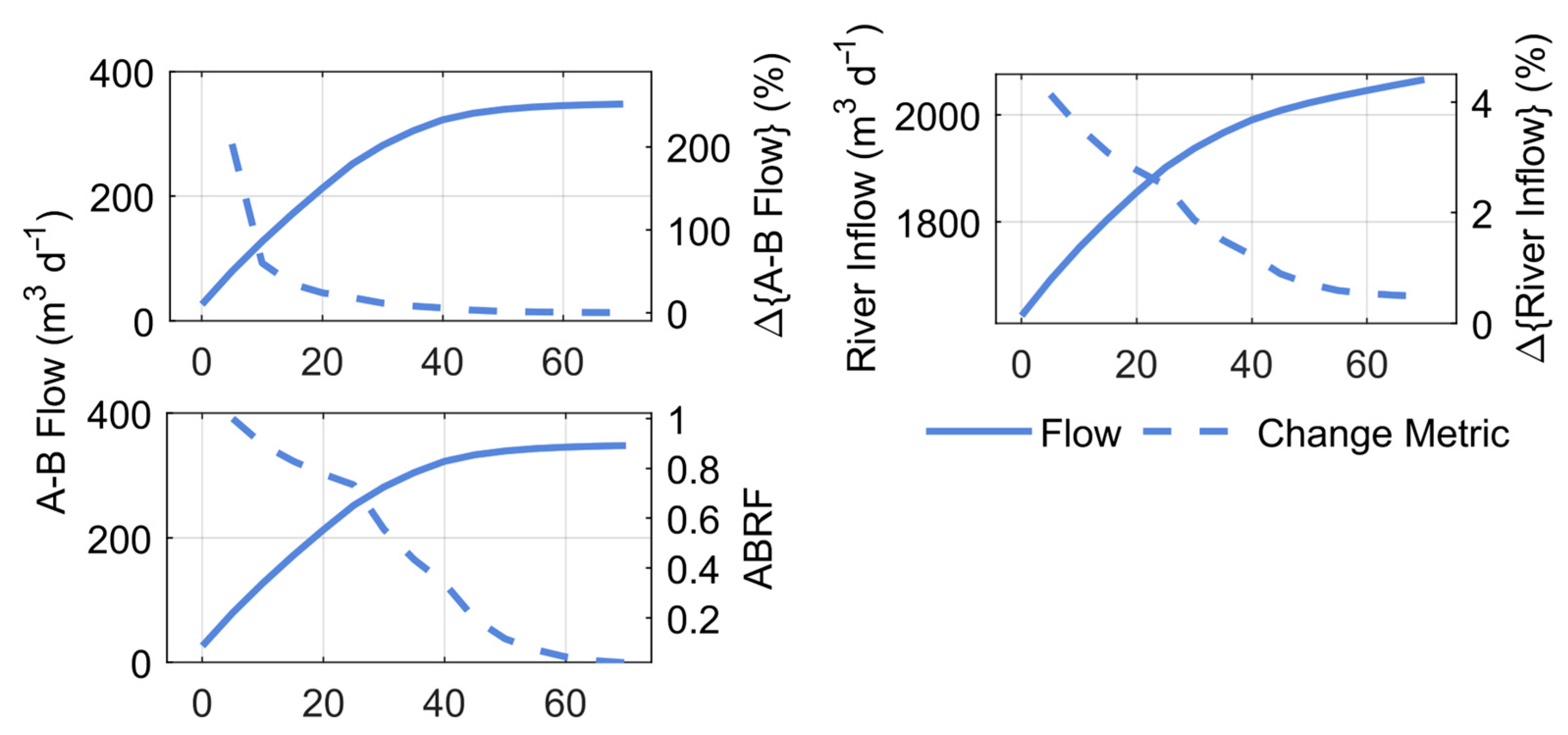
3.2. Inter-Aquifer Flow and Seepage

The simulated alluvial-to-bedrock (A-B) flow and river inflow (seepage integrated over all river cells) ranged from 26 to 347 m³ day⁻¹ and 1624 to 2066 m³ day⁻¹, respectively. During the transient simulation, some induced stream recharge (Δ river inflow) bypassed A-B flow, exiting the model domain via the alluvial aquifer. Both flow rates increased with regional water table lowering, initially following a linear trend, and then progressively flattening with successive water table lowering. The percentage change in flow rate between stress periods (Δ{A-B Flow}) decreased rapidly at the beginning of the simulation and approached 0% and 0.5% at the simulation end for A-B flow and river inflow, respectively. Similarly, ABRF starts at 1 (by definition) and progressively decreases over time to a final value of 0.019, indicating a 98% reduction in the flow response. In years 25–30, ABRF shows a distinct slope change at the onset of unsaturated conditions, demonstrating the utility of this metric for detecting the onset of a transitional regime (Figure 4). In year 50, ABRF begins to flatten, indicating minimal flow change with successive water table lowering. For the remainder of the simulation, ABRF asymptotically approaches zero, indicating hydraulic disconnection.

3.3. Sensitivity to Sandstone Channel Architecture

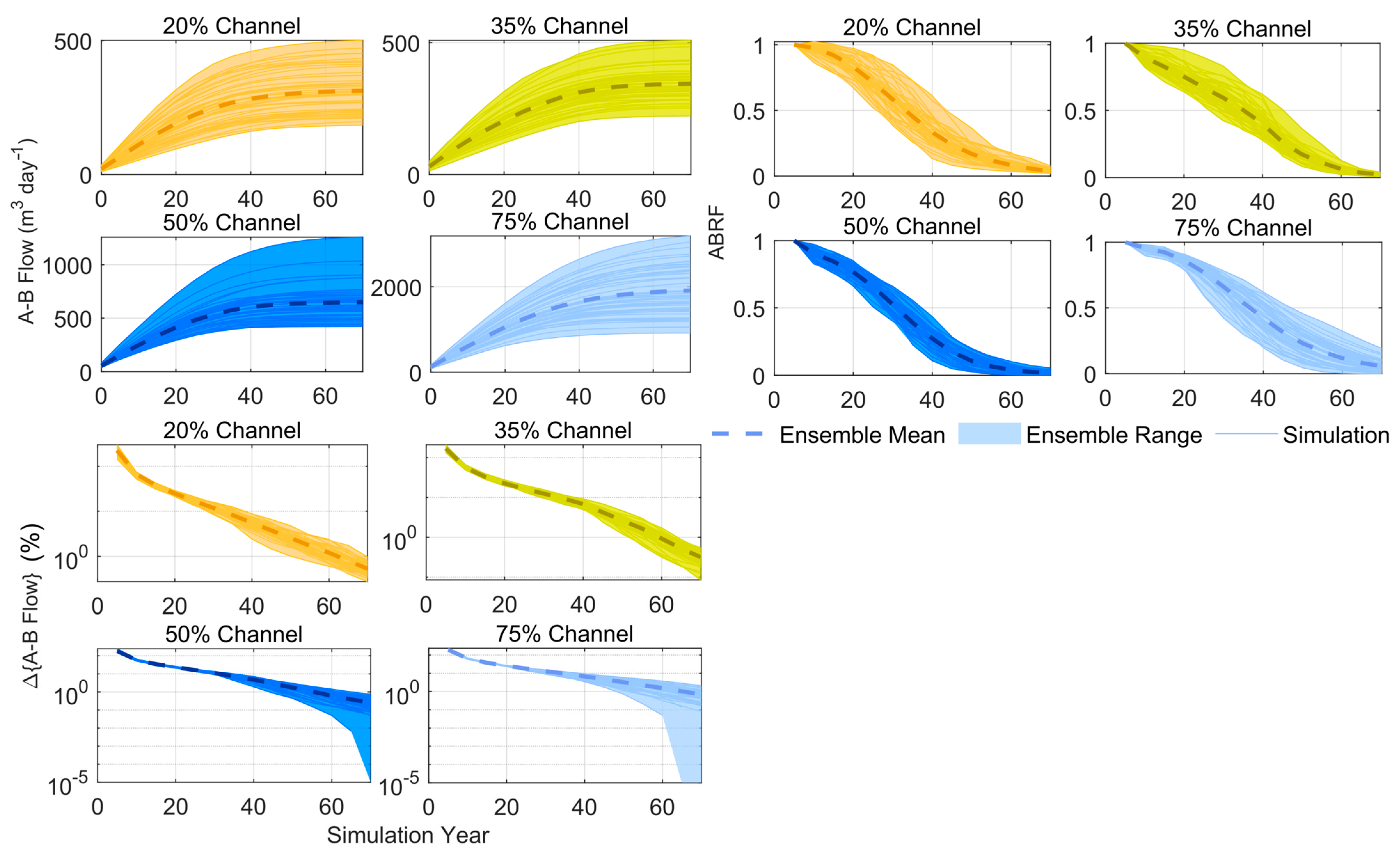
3.3.1. A-B Flow

Across all simulations and channel fractions, A-B flow, Δ{A-B Flow}, and ABRF show similar behavior to the representative scenario (Figure 5). The final A-B flow rates ranged from 184 to 3187 m³ day⁻¹ with ensemble mean values of 313, 344, 650, and 1913 m³ day⁻¹ for channel fractions of 20%, 35%, 50%, and 75%, respectively (

Table 2. Summary of model results for final timestep (year 70) for all simulations.

		Ensemble Mean	Minimum	Maximum	σ	CV
A-B Flow (m3 day−1)	20%	313	184	501	81	0.26
	35%	344	222	508	60	0.17
	50%	650	423	1258	154	0.24
	75%	1913	919	3187	554	0.29
Δ{A-B Flow}	20%	0.53	0.27	0.97	0.15	0.28
	35%	0.32	0.085	0.55	0.10	0.31
	50%	0.25	−0.010	0.74	0.16	0.64
	75%	0.68	−0.040	2.1	0.45	0.66
ABRF	20%	0.037	0.018	0.075	0.012	0.34
	35%	0.022	0.0058	0.040	0.0074	0.34
	50%	0.016	−0.00080	0.054	0.011	0.69
	75%	0.055	−0.0027	0.19	0.040	0.74

). The standard deviation (σ) and coefficient of variation (CV) of the final A-B flow rates, ranging from 60 to 554 m³ per day⁻¹ and from 0.17 to 0.29, respectively, were greater for higher channel fractions except for the 20% scenarios, generally indicating a greater range in final flow across simulations with greater sandstone fractions. The 20% scenarios had greater σ and CV values than the 35% scenarios, which may be related to the 20% scenarios being unconstrained by geophysical log data. As in the example scenario, all simulations are characterized by flow increasing linearly at first and then flattening with successive water table lowering. Some simulations show more pronounced flattening than others, while simulations with a lower final A-B flow rate tend to have a flatter final slope.

The A-B flow rate positively correlates with both the fraction of flow through sandstone channels and river inflow (Figure S6 in Supporting Information). Higher flow rates occur when a greater proportion of flow is channeled through sandstone. Additionally, increased vertical flow, indicative of a more transmissive aquifer at depth, enhances stream seepage.

3.3.2. A-B Flow Percentage Change

The final A-B flow percentage change (Δ{A-B Flow}) ranged from −0.04 to 2.1%, with ensemble means of 0.53%, 0.32%, 0.25%, and 0.68% for channel fractions of 20%, 35%, 50%, and 75%, respectively (Table 2). A negative percent change signifies a decrease in the A-B flow rate between successive timesteps, suggesting stabilizing A-B flow rates and hydraulic disconnection. The ensemble mean showed no clear trend with channel fraction. Most simulations had a final Δ{A-B Flow} below 1%, indicating minimal flow change with successive lowering, except for ten 75% channel fraction scenarios. The σ value, ranging from 0.1 to 0.45, and CV, ranging from 0.28 to 0.66, generally increased with channel fraction, indicating greater variability at higher fractions. As in the representative scenario, Δ{A-B Flow} decreased rapidly in the first 10 years and then asymptotically approached zero for the duration of the simulations.

3.3.3. Alluvial-to-Bedrock Flow Response Function

The final ABRF values ranged from −0.0008 to 0.19, with ensemble means of 0.037, 0.022, 0.16, and 0.055 for channel fractions of 20%, 35%, 50%, and 75%, respectively (Table 2). Negative values indicate a decrease in A-B flow between successive timesteps, suggesting stabilizing flow and hydraulic disconnection. The ensemble mean ABRF increased slightly with channel fraction, excluding 20% realizations. The 75% channel fraction exhibited the largest ABRF range (−0.0027 to 0.19), indicating final flow responses ranging from 0.27% to 19% of the initial flow, depending on bedrock aquifer heterogeneity. The σ value, ranging from 0.007 to 0.04, and CV, ranging from 0.34 to 0.74, generally increased with channel fraction, again excluding 20%. The ABRF trends mirrored the representative scenario, with the most significant changes occurring between 20 and 40 years and gradual decreases occurring thereafter.

3.4. Connectivity Structure of Heterogeneity

Initial assessments revealed that no single static or dynamic connectivity metric independently predicted the final A-B flow rate. To determine whether a combination of metrics could better explain variations in the final A-B flow, multiple linear regression (MLR) analysis was conducted. All connectivity metrics were initially included as predictor variables, and insignificant predictors (high p-value) were iteratively removed. The resulting MLR coefficients and model fits demonstrate statistically significant predictive power (p < 0.05), with R² values ranging from 0.52 to 0.88, indicating that the models explained a substantial portion of the variability in A-B flow rates (

Table 3. Results from multiple linear regression analysis performed for each channel fraction (all model realizations considered) using significant predictor variables A-B_{SS_%}, MCC_DY, NCC_DY, ZCC_DY, and ABZCC_DY and response variable of A-B flow (m³ day⁻¹).

Channel Fraction	Predictor				Model
		Estimate	1 SE	p-Value	2 RMSE	3 R-Squared	p-Value
20%	Intercept	153	48	4 2.67 × 10–3	56.7	0.52	4.0 × 10–7
	A-BSS_%	3	0.7	2.78 × 10–4
	MCCDY	0.0010	0.0005	5.27 × 10–2
	NCCDY	−1.1	1.03	2.80 × 10–1
	ZCCDY	−2	1.8	2.14 × 10–1
	ABZCCDY	3	1.6	8.26 × 10–2
35%	Intercept	3	62	9.63 × 10–1	39.8	0.57	4.3 × 10–8
	A-BSS_%	2.7	0.5	4.71 × 10–6
	MCCDY	3.2 × 10−5	1.7E-04	8.49 × 10–1
	NCCDY	−0.028	0.4	9.47 × 10–1
	ZCCDY	0.5	0.8	5.32 × 10–1
	ABZCCDY	5	0.8	6.88 × 10–8
50%	Intercept	100	124	4.24 × 10–1	104	0.56	6.0 × 10–8
	A-BSS_%	6	1.2	2.55 × 10–5
	MCCDY	0.0019	0.0005	4.78 × 10–4
	NCCDY	−2.6	1.0	1.04 × 10–2
	ZCCDY	−5	1.3	8.53 × 10–4
	ABZCCDY	1.06	0.6	7.04 × 10–2
75%	Intercept	403	408	3.29 × 10–1	193	0.88	3.1 × 10–20
	A-BSS_%	−5	4	1.95 × 10–1
	MCCDY	0.010	0.00079	3.76 × 10–6
	NCCDY	−2.5	2.2	2.73 × 10–1
	ZCCDY	−34	4	6.26 × 10–11
	ABZCCDY	3	2.1	1.56 × 10–1

Note(s): ¹ SE is the standard error. ² RMSE is the root mean square error. ³ The R² value is adjusted for the number of predictors in the model. ⁴ Significant p-values at the 95% confidence level are bolded.

). The most significant predictors, in descending order of importance, were A-B_{SS_%}, ZCC_DY, ABZCC_DY, NCC_DY, and MCC_DY. Notably, the predictive power of sandstone connectivity increased with higher sandstone channel fractions, suggesting that sandstone connectivity is a stronger determinant of A-B fluxes for higher sandstone fractions.

A similar MLR analysis was performed to predict the ABRF. The same connectivity metrics identified for A-B flow rate prediction were also significant predictors of ABRF. Although the R² values were generally lower (0.17 to 0.59), they exhibited a similar trend of increasing with higher channel fraction, highlighting the dominant influence of channel connectivity on disconnection dynamics with greater sandstone fraction. Detailed results from this analysis are presented in the Supporting Information (Table S2). Comprehensive connectivity results for all metrics are detailed in the Supporting Information (Figures S7 and S8).

4. Discussion

This study combines geostatistical methods and variably saturated flow modeling to evaluate the influence of unsaturated zone development on flow between two aquifers. The results provide valuable insights for pumped aquifer dynamics and associated implications for management.

4.1. Disconnection Dynamics

In this study, numerical modeling revealed the development of unsaturated regions between the alluvium and bedrock in all scenarios, indicating that a transitional flow regime developed in all simulations. A disconnected flow regime is defined as the state where successive water table declines no longer significantly impact flux, which asymptotically approaches a constant maximum value. Given the asymptotic nature of the maximum flow rate, distinguishing transitional from disconnected systems necessitates an arbitrary cutoff value for which changes are deemed negligible. To differentiate between transitional and disconnected regimes, we applied a practical cutoff of Δ{A-B Flow} < 1%, classifying simulations below this threshold as disconnected. This flow change represents negligible change in flow despite water table lowering. Using this criterion, 190 of the 200 simulations exhibited hydraulic disconnection between the alluvial and bedrock aquifer, with the remaining 10 transitional scenarios being associated with 75% bedrock channel fractions. The ABRF for this cutoff was 0.08, demonstrating that disconnected systems experienced a flow reduction of 92% compared to fully connected conditions.

The simulated flow rates from the alluvial to bedrock aquifer exhibited a more gradual transition compared to similar studies that modeled the effects of unsaturated conditions on near-surface infiltration and recharge. Previous research often reported an abrupt transition from a linear flow trend in connected conditions to a flattened curve at disconnection (e.g., [2,28]). In contrast, our results show an initial linear period followed by prolonged transitional phase that smoothly grades into disconnection.

Several factors may explain the extended transitional phase observed in our models. The complex and dynamic nature of saturation and hydraulic conductivity fields, which change throughout the simulation due to varying pressure, likely contributes to the response. Given the influence of heterogeneity on flow, flow rates are unlikely to stabilize before the saturation-dependent heterogeneity field also reaches stability. Furthermore, previous studies often employed relatively homogeneous fields with a single clogging unit, e.g., [17,22] or limited the analysis to 1D and 2D model domains, e.g., [4,9,17,28]. Greater heterogeneity has been found to significantly affect exchange rates, pressure heads, and the state of connection/disconnection [17]. Compared to analogous 3D heterogeneity fields with comparable statistics and architecture, 2D fields typically exhibit lower connectivity [18]. The dynamic 3D heterogeneity implemented in this study resulted in spatially variable saturation patterns and connection status across the model domain, thereby producing smoother total A-B flow rates over time.

The transient nature of the VSF model simulations in this study may also contribute to the smooth, prolonged transitional phase. This contrasts with fundamental reviews of stream–aquifer disconnection, which have often relied on steady-state simulations [2,21,22]. Transient models inherently account for the lag time associated with changes in saturation and pressure head, consequently impacting flow dynamics. Previous studies have demonstrated the influence of these lag times on recharge rates in unsaturated conditions [3]. Therefore, transient simulations are expected to produce smoother, more gradual flow rate transitions.

4.2. Heterogeneity Controls for Inter-Aquifer Flow

The results demonstrate a significant influence of geologic heterogeneity on aquifer exchange rates under scenarios of water table lowering. The A-B interface sandstone fraction (A-B_{SS_%}) emerged as the strongest predictor of the final A-B flow rate in all but the 75% channel fraction MLR. The A-B flow rates increased with increasing sandstone presence at the A-B interface, which is consistent with the expectation that sandstone provides a high-permeability conduit for preferential flow. In simulations with 20% channel fraction, the absence of sandstone at the A-B interface resulted in the lowest A-B flow rates. Interestingly, the significance of A-B_{SS_%} diminished in the 75% channel simulations, suggesting that beyond a certain threshold, additional sandstone at the interface no longer significantly enhances the exchange rate.

The remaining significant predictors, ZCC_DY and ABZCC_DY, are dynamic connectivity metrics that reflect the spatial distribution of saturation-dependent hydraulic conductivity. These metrics represent the maximum vertical extent of connected components, both generally and specifically contacting the alluvium. The ZCC_DY had predictive power only when negative, suggesting that higher A-B flow rates occurred with lower saturated vertical connectivity. This is the opposite of what was expected. One possible explanation is that thinner connected sandstones prohibit the formation of unsaturated zones, thereby resulting in greater final flow rates. Conversely, the ABZCC_DY coefficient is positive, indicating that thicker saturated sandstone bodies contacting the alluvium are correlated with higher A-B flow rates. This result is consistent with the finding that thick saturated sandstones contacting the alluvium effectively thicken the shallow saturated zone, leading to greater A-B flow rates.

The NCC_DY exhibited a consistent negative coefficient across all MLRs, indicating an inverse relationship between the number of connected components and the final A-B flow rate. This suggests that a greater number of individual connected components, typically associated with lower overall connectivity, resulted in diminished flow. Conversely, MCC_DY demonstrated the smallest coefficient and varied in sign (positive and negative) across simulations, without a discernable trend. This result is counterintuitive, as larger connected components would intuitively be expected to enhance A-B flow. However, larger sandstone bodies may also be more susceptible to desaturation, complicating the interpretation of this metric. Consequently, the relationship between MCC_DY and A-B flow rates remains inconclusive.

Saturated volumes of alluvium, sandstone, and mudstone were plotted for multiple realizations to elucidate the relationship between flow, saturation, and heterogeneity. Realizations with lower bedrock sandstone fractions (≤35%) exhibited substantial saturated mudstone volumes underlying the alluvium along with dispersed saturated sandstone channels amounting to minimal sandstone being present at the alluvium–bedrock contact (e.g., Figure 6a). This lack of sandstone at the A-B interface forced flow through the low-permeability mudstone, thereby restricting A-B flow. Conversely, realizations with greater sandstone fractions (≥50%) displayed predominantly sandstone saturation in the bedrock, with minimal saturated mudstone, indicating flow primarily through sandstone. Multiple interconnected channels spanning the model domain (and intersecting the alluvium) facilitated both lateral and vertical A-B exchange, resulting in greater A-B flow. Lower A-B flow rates often occurred when sandstone “pinch points” channeled flow into a single, narrow conduit spanning the vertical domain. While the factors dictating pinch point occurrence remain unclear from evaluated metrics, fluvial architecture demonstrably controlled the saturated zone geometry and associated recharge conduits. These findings corroborate the observation that realizations with lower sandstone fractions tend to have less sandstone at the A-B contact and lower A-B flow rates overall.

Mudstone units underlying the alluvium exhibit analogous behavior to clogging layers described in groundwater–surface water disconnection studies. Brunner et al. [2,22] highlighted the impact of aquifer and clogging layer thickness ratios on unsaturated zone development. They concluded that thicker clogging units promote desaturation, while a thin aquifer layer relative to the clogging layer inhibits it. Our study reveals a similar trend, with realizations featuring thick saturated mudstone units and relatively thin sandstones being less likely to desaturate (Figure 6a). Conversely, realizations characterized by large, highly connected sandstone units and thin mudstones tended to develop large unsaturated zones (Figure 6b) and lower final A-B flow rates compared to other realizations with the same sandstone fraction.

Volume plots further revealed important dynamics at the alluvium–bedrock contact. Realizations with increased sandstone contact at the alluvium displayed thicker and wider perched saturated zones (Figure 6c,d). Thicker perched zones facilitated increased pressure development at the perched zone base, enhancing flow through underlying units. This relates to similar findings beneath streambeds wherein evolving the geometry of the unsaturated zone controlled both the time to disconnection and maximum infiltration rates [30].

According to Brunner et al. [21], a 1D system with an aquifer underlying a clogging layer may begin to desaturate if the following conditions are met:

$${\displaystyle \frac{K_c}{K_a}}\le {\displaystyle \frac{b_c}{d+b_c}}$$

(5)

where K_c and b_c are the clogging layer hydraulic conductivity (LT⁻¹) and thickness (L), K_a is the aquifer hydraulic conductivity (LT⁻¹), and d is the surface water depth (L). When applying this 1D analogy and holding all other parameters constant, increasing the thickness of the saturated alluvium reduces the potential for unsaturated conditions. Consequently, increased pressure transfer from thicker perched zones to underlying units diminished the likelihood of negative pressure development. Furthermore, sandstone units extending to lateral edges of the alluvium tended to remain saturated, effectively widening the perched aquifer and increasing the probability of intersecting underlying channels. Realizations with the highest A-B flow rates exhibited these wider perched zones.

Connected component analysis demonstrated that static and dynamic heterogeneity fields in realizations with sandstone fractions ≥ 50% exhibited connected bodies spanning the vertical model domain, predicting distinct flow behavior compared to realizations with lower sandstone fractions. This prediction was validated by comparing simulation results across varying channel fractions (Table 2). Regression analysis indicated that the ZCC_DY connectivity metric became increasingly predictive of A-B flow for 50% and 75% sandstone fractions (Table 3), with overall connectivity metrics showing improved A-B flow prediction with increasing bedrock channel fractions. These results suggest that A-B flow is increasingly controlled by high-permeability unit connectivity, particularly vertically spanning channel bodies as bedrock channel fraction increases.

In summary, although 1D analytical models [21] or 2D numerical flow models may accurately predict the potential for disconnection [28], our findings highlight the need to consider the 3D dynamic connectivity structure to accurately represent flow paths and determine the maximum inter-aquifer exchange rate.

4.3. Definition of Disconnection

Current definitions for disconnected flow regimes primarily focus on surface water bodies (e.g., [2,21,22]). This study demonstrates a novel scenario where, despite the connection between a stream and shallow aquifer, an unsaturated zone develops between deeper aquifers within the system. Consequently, further water table lowering in the deeper aquifer no longer substantially impacts the inter-aquifer exchange rate. To our knowledge, the Denver Basin is one of the few, if only, places where this phenomenon has been considered [28]. While previous research has described the development of stable stream seepage and perched aquifer conditions with declining deeper water tables, e.g., [48,51], our work specifically addresses the stabilization of exchange rates between two aquifers. Therefore, the definition of disconnected flow regimes should be expanded to encompass settings beyond the groundwater–surface water interface.

4.4. Management Implications

As demonstrated, both transitional and disconnected flow regimes exhibit significantly lower recharge rates compared to fully saturated systems (Figure 4 and Figure 5). Failure to account for this diminished recharge in predictive models could result in overestimates of aquifer storage and recharge, leading to inaccurate projections of future groundwater conditions. Consequently, such models may produce erroneous determinations of sustainable pumping yields and inflated estimates of future water availability. Furthermore, in regions such as the Denver Basin, where water use is governed by water rights, inaccurate estimates of aquifer exchange rates could negatively impact groundwater extraction rights, potentially resulting in inequitable water allocation [26].

This study highlights the necessity of detailed numerical modeling, incorporating explicit 3D representation of heterogeneity, to accurately determine the occurrence, location, and extent of hydraulic disconnection. Inter-aquifer flow rates resulting from water table drawdown are sensitive to heterogeneity, particularly the spatial connectivity and presence of high-permeability units at the alluvial–bedrock contact (Table 3). Regional-scale models used to evaluate pumping impacts are often limited to coarse-grid resolutions and effective upscaled parameters and may be inadequate for reliably simulating processes that are strongly influenced by heterogeneity. Therefore, we demonstrate how detailed modeling with explicit representation of heterogeneity is critical for determining inter-aquifer flow dynamics in heterogeneous aquifers with significant water table drawdown (i.e., long-term pumping).

Analogous to stream–aquifer scenarios, disconnection between alluvial and bedrock aquifers does not imply that A-B flow rates are unaffected by additional stresses within the system. Similarly to how pumping near a disconnected stream can expand the extent of disconnection [1], increased pumping in the bedrock aquifer could extend the spatial extent of inter-aquifer disconnection. Furthermore, changes in streamflow can affect stream–aquifer exchange despite disconnection [52,53]; similarly, changes in alluvial groundwater levels or other aquifer stress conditions could affect inter-aquifer exchange even with established disconnection.

Historically depleted aquifer systems are potential sites for managed aquifer recharge [54,55,56]. In some instances, these sites have experienced hydraulic disconnection. Numerical modeling efforts, similar to the approach used in this study, may be useful for evaluating the responses of these systems to recharge operations.

5. Conclusions

This study reveals that progressive water table lowering in multi-aquifer systems can result in hydraulic disconnection, thereby limiting the amount of induced recharge from a shallow aquifer unit. Three-dimensional, transient, variably saturated flow modeling, incorporating diverse realizations of fluvial heterogeneity, revealed the development and propagation of unsaturated zones that led to a substantial curtailment of alluvial-to-bedrock (A-B) flow. The percentage change in flow and normalized response function revealed a 98% reduction in the flow induced by drawdown and facilitated a cross-scenario comparison of inter-aquifer flow changes. The results revealed that 190 out of 200 simulations reached full disconnection (percentage change of <1% with successive water table lowering), while the remaining 10 exhibited transitional behavior approaching disconnection.

Heterogeneity within the bedrock aquifer, particularly the amount of high-permeability sandstone channels at the alluvial–bedrock aquifer interface and the vertical span of saturated, connected sandstones, critically controlled the maximum alluvial-to-bedrock flow rate and transition to disconnection. Specifically, channel locations dictated the formation and geometry of unsaturated regions and perched saturated zones, which either restricted or facilitated A-B flow by altering the effective saturated hydraulic conductivity. These findings underscore the need to consider the saturation state and the explicit 3D representation of heterogeneity to accurately determine inter-aquifer exchange rates in heavily pumped multi-aquifer systems.

Hydraulic disconnection can significantly reduce inter-aquifer flow and recharge, and neglecting this in predictive models can lead to overestimations of groundwater availability and potentially inequitable water allocation, particularly in heavily pumped regions. Failure to account for diminished recharge could result in overestimates of aquifer storage and recharge, leading to inaccurate projections of future groundwater conditions, sustainability calculations, and water rights determinations. Furthermore, by demonstrating hydraulic disconnection between a shallow and deep aquifer, this study expands the current understanding of this phenomenon and provides a representative case study for hydraulic disconnection between aquifers. These findings underscore the necessity of incorporating heterogeneity and unsaturated flow processes into finer-scale models to inform regional groundwater models and management in complex aquifer systems.

References

1. Fox, G.A.; Durnford, D.S. Unsaturated hyporheic zone flow in stream/aquifer conjunctive systems. Adv. Water Resour. 2003, 26, 989–1000. [Google Scholar] [CrossRef]
2. Brunner, P.; Cook, P.G.; Simmons, C.T. Disconnected surface water and groundwater: From theory to practice. Groundwater 2011, 49, 460–467. [Google Scholar] [CrossRef] [PubMed]
3. Hunt, R.J.; Prudic, D.E.; Walker, J.F.; Anderson, M.P. Importance of unsaturated zone flow for simulating recharge in a humid climate. Groundwater 2008, 46, 551–560. [Google Scholar] [CrossRef]
4. Desilets, S.L.E.; Ferre, T.P.A.; Troch, P.A. Effects of stream-aquifer disconnection on local flow patterns. Water Resour. Res. 2008, 44, W09501. [Google Scholar] [CrossRef]
5. Shanafield, M.; Cook, P.G.; Brunner, P.; McCallum, J.; Simmons, C.T. Aquifer response to surface water transience in disconnected streams. Water Resour. Res. 2012, 48. [Google Scholar] [CrossRef]
6. Theis, C.V. The effect of a well on the flow of a nearby stream. Eos Trans. Am. Geophys. Union 1941, 22, 734–738. [Google Scholar] [CrossRef]
7. Su, G.W.; Jasperse, J.; Seymour, D.; Constantz, J.; Zhou, Q. Analysis of pumping-induced unsaturated regions beneath a perennial river. Water Resour. Res. 2007, 43, W08421. [Google Scholar] [CrossRef]
8. Frei, S.; Fleckenstein, J.H.; Kollet, S.J.; Maxwell, R.M. Patterns and dynamics of river–aquifer exchange with variably-saturated flow using a fully-coupled model. J. Hydrol. 2009, 375, 383–393. [Google Scholar] [CrossRef]
9. Swanson, S.K.; Bahr, J.M.; Bradbury, K.R.; Anderson, K.M. Evidence for preferential flow through sandstone aquifers in Southern Wisconsin. Sediment. Geol. 2006, 184, 331–342. [Google Scholar] [CrossRef]
10. Maples, S.R.; Foglia, L.; Fogg, G.E.; Maxwell, R.M. Sensitivity of hydrologic and geologic parameters on recharge processes in a highly heterogeneous, semi-confined aquifer system. Hydrol. Earth Syst. Sci. 2020, 24, 2437–2456. [Google Scholar] [CrossRef]
11. Fleckenstein, J.H.; Niswonger, R.G.; Fogg, G.E. River-aquifer interactions, geologic heterogeneity, and low-flow management. Groundwater 2006, 44, 837–852. [Google Scholar] [CrossRef]
12. Meier, P.M.; Carrera, J.; Sánchez-Vila, X. An evaluation of Jacob’s method for the interpretation of pumping tests in heterogeneous formations. Water Resour. Res. 1998, 34, 1011–1025. [Google Scholar] [CrossRef]
13. Knudby, C.; Carrera, J. On the use of apparent hydraulic diffusivity as an indicator of connectivity. J. Hydrol. 2006, 329, 377–389. [Google Scholar] [CrossRef]
14. Dann, R.L.; Close, M.E.; Pang, L.; Flintoft, M.J.; Hector, R.P. Complementary use of tracer and pumping tests to characterize a heterogeneous channelized aquifer system in New Zealand. Hydrogeol. J. 2008, 16, 1177–1191. [Google Scholar] [CrossRef]
15. Ronayne, M.J.; Gorelick, S.M.; Caers, J. Identifying discrete geologic structures that produce anomalous hydraulic response: An inverse modeling approach. Water Resour. Res. 2008, 44, W08426. [Google Scholar] [CrossRef]
16. DesRoches, A.J.; Butler, K.E.; Pelkey, S. Influence of fracture anisotropy and lithological heterogeneity on wellfield response in a fluvial sandstone aquifer of the Carboniferous Moncton Subbasin, Canada. Hydrogeol. J. 2013, 21, 559. [Google Scholar] [CrossRef]
17. Tang, Q.; Kurtz, W.; Schilling, O.S.; Brunner, P.; Vereecken, H.; Franssen, H.J.H. The influence of riverbed heterogeneity patterns on river-aquifer exchange fluxes under different connection regimes. J. Hydrol. 2017, 554, 383–396. [Google Scholar] [CrossRef]
18. Bruen, M.P.; Osman, Y.Z. Sensitivity of stream–aquifer seepage to spatial variability of the saturated hydraulic conductivity of the aquifer. J. Hydrol. 2004, 293, 289–302. [Google Scholar] [CrossRef]
19. Renard, P.; Allard, D. Connectivity metrics for subsurface flow and transport. Adv. Water Resour. 2013, 51, 168–196. [Google Scholar] [CrossRef]
20. Rosenberry, D.O. Unsaturated-zone wedge beneath a large, natural lake. Water Resour. Res. 2000, 36, 3401–3409. [Google Scholar] [CrossRef]
21. Brunner, P.; Cook, P.G.; Simmons, C.T. Hydrogeologic controls on disconnection between surface water and groundwater. Water Resour. Res. 2009, 45, W01422. [Google Scholar] [CrossRef]
22. Brunner, P.; Simmons, C.T.; Cook, P.G. Spatial and temporal aspects of the transition from connection to disconnection between rivers, lakes and groundwater. J. Hydrol. 2009, 376, 159–169. [Google Scholar] [CrossRef]
23. Schilling, O.S.; Irvine, D.J.; Hendricks Franssen, H.J.; Brunner, P. Estimating the spatial extent of unsaturated zones in heterogeneous river-aquifer systems. Water Resour. Res. 2017, 53, 10583–10602. [Google Scholar] [CrossRef]
24. Wada, Y.; Van Beek, L.P.; Van Kempen, C.M.; Reckman, J.W.; Vasak, S.; Bierkens, M.F. Global depletion of groundwater resources. Geophys. Res. Lett. 2010, 37, L20402. [Google Scholar] [CrossRef]
25. Werner, A.D.; Zhang, Q.; Xue, L.; Smerdon, B.D.; Li, X.; Zhu, X.; Yu, L.; Li, L. An initial inventory and indexation of groundwater mega-depletion cases. Water Resour. Manag. 2013, 27, 507–533. [Google Scholar] [CrossRef]
26. Paschke, S.S. (Ed.) Groundwater Availability of the Denver Basin Aquifer System; U.S. Geological Survey Professional Paper 1770; U.S. Geological Survey: Reston, VA, USA, 2011; 274p. [CrossRef]
27. Ruybal, C.J.; Hogue, T.S.; McCray, J.E. Assessment of groundwater depletion and implications for management in the Denver basin aquifer system. J. Am. Water Resour. Assoc. 2019, 55, 1130–1148. [Google Scholar] [CrossRef]
28. Cognac, K.E.; Ronayne, M.J. Changes to inter-aquifer exchange resulting from long-term pumping: Implications for bedrock groundwater recharge. Hydrogeol. J. 2020, 28, 1359–1370. [Google Scholar] [CrossRef]
29. Ronayne, M.J.; Gorelick, S.M.; Zheng, C. Geological modeling of submeter scale heterogeneity and its influence on tracer transport in a fluvial aquifer. Water Resour. Res. 2010, 46, W10519. [Google Scholar] [CrossRef]
30. Irvine, D.J.; Brunner, P.; Franssen, H.J.H.; Simmons, C.T. Heterogeneous or homogeneous? Implications of simplifying heterogeneous streambeds in models of losing streams. J. Hydrol. 2012, 424, 16–23. [Google Scholar] [CrossRef]
31. Deutsch, C.A.; Tran, T.T. FLUVSIM: A program for object-based stochastic modeling of fluvial depositional systems. Comput. Geosci. 2002, 28, 525–535. [Google Scholar] [CrossRef]
32. Raynolds, R.G. Upper Cretaceous and Tertiary stratigraphy of the Denver basin, Colorado. Rocky Mt. Geol. 2002, 37, 111–134. [Google Scholar] [CrossRef]
33. Panday, S.; Langevin, C.D.; Niswonger, R.G.; Ibaraki, M.; Hughes, J.D. MODFLOW-USG: An Unstructured Grid Version of MODFLOW for Simulating Groundwater Flow and Tightly Coupled Processes Using a Control Volume Finite-Difference Formulation; Version 1; U.S. Geological Survey Techniques and Methods: Reston, VA, USA, 2013. [CrossRef]
34. Panday, S. USG-Transport: The Block-Centered Transport Process for MODFLOW-USG; Version 1.4.0; GSI Environmental: Houston, TX, USA, 2019; Available online: https://www.gsi-net.com/en/software/free-software/USG-Transport.html (accessed on 1 May 2023).
35. Hort, H.M.; Stockwell, E.B.; Newell, C.J.; Scalia, J., IV; Panday, S. Modeling and evaluation of PFOS retention in the unsaturated zone above the water table. Groundw. Monit. Remediat. 2024, 44, 38–48. [Google Scholar] [CrossRef]
36. Vonk, M.A.; Collenteur, R.A.; Panday, S.; Schaars, F.; Bakker, M. Time Series Analysis of Nonlinear Head Dynamics Using Synthetic Data Generated with a Variably Saturated Model. Groundwater 2024, 62, 748–760. [Google Scholar] [CrossRef]
37. Huyakorn, P.S.; Springer, E.P.; Guvanasen, V.; Wadsorth, T.D. A three dimensional finite element model for simulating water flow in variably saturated porous media. Water Resour. Res. 1986, 22, 1790–1808. [Google Scholar] [CrossRef]
38. van Genuchten, M.T. A closed-form equation for predicting the hydraulic conductivity of unsaturated soils. Soil. Sci. Soc. Am. J. 1980, 44, 892–898. [Google Scholar] [CrossRef]
39. Brooks, R.H.; Corey, A.T. Properties of porous media affecting fluid flow. J. Irrig. Drain. Div. 1966, 92, 61–88. [Google Scholar] [CrossRef]
40. Harbaugh, A.W.; Banta, E.R.; Hill, M.C.; McDonald, M.G. Geological Survey Modular Ground-Water Model—User Guide to Modularization Concepts and the Ground-Water Flow Process; US Geological Survey Open-File Report; U.S. Geological Survey: Reston, VA, USA, 2000. [CrossRef]
41. Colorado Division of Water Resources (CDWR). State Water Level Database, Colorado Government. 2022. Available online: https://dwr.state.co.us/Tools/GroundWater/WaterLevels (accessed on 17 November 2022).
42. Lapey, L.A. Hydrogeologic Parameters of the Kiowa Research Core, Kiowa, Colorado. Master’s Thesis, Colorado State University, Fort Collins, CO, USA, 2001. [Google Scholar]
43. Woodard, L.; Sanford, W.; Raynolds, R.G. Stratigraphic variability of specific yield within bedrock aquifers of the Denver Basin, Colorado. Rocky Mt. Geol. 2002, 37, 229–236. [Google Scholar] [CrossRef]
44. Brown and Caldwell. South Platte Decision Support System Alluvial Groundwater Model Update Documentation; Colorado Water Conservation Board and Division of Water Resources: Denver, CO, USA, 2017.
45. Carsel, R.F.; Parrish, R.S. Developing joint probability distributions of soil water retention characteristics. Water Resour. Res. 1988, 24, 755–769. [Google Scholar] [CrossRef]
46. Parajuli, K.; Sadeghi, M.; Jones, S.B. A binary mixing model for characterizing stony-soil water retention. Agric. For. Meteorol. 2017, 244, 1–8. [Google Scholar] [CrossRef]
47. Morel-Seytoux, H.J.; Meyer, P.D.; Nachabe, M.; Tourna, J.; Van Genuchten, M.T.; Lenhard, R.J. Parameter equivalence for the Brooks-Corey and van Genuchten soil characteristics: Preserving the effective capillary drive. Water Resour. Res. 1996, 32, 1251–1258. [Google Scholar] [CrossRef]
48. Harbaugh, A.W. A Computer Program for Calculating Subregional Water Budgets Using Results from the U.S. Geological Survey Modular Three-Dimensional Ground-Water Flow Model; U.S. Geological Survey: Reston, VA, USA, 1990; 46p. [CrossRef]
49. King, P.R. The connectivity and conductivity of overlapping sand bodies. In North Sea Oil and Gas Reservoirs—II, Proceedings of the 2nd North Sea Oil and Gas Reservoirs Conference organized and hosted by the Norwegian Institute of Technology (NTH), Trondheim, Norway, 8–11 May 1989; Springer: Dordrecht, The Netherlands, 1990; pp. 353–362. [Google Scholar] [CrossRef]
50. Pardo-Iguzquiza, E.; Dowd, P. CONNEC3D: A computer program for connectivity analysis of 3D random set models. Comput. Geosci. 2003, 29, 775–785. [Google Scholar] [CrossRef]
51. Rains, M.C.; Fogg, G.E.; Harter, T.; Dahlgren, R.A.; Williamson, R.J. The role of perched aquifers in hydrological connectivity and biogeochemical processes in vernal pool landscapes, Central Valley, California. Hydrol. Process. 2006, 20, 1157–1175. [Google Scholar] [CrossRef]
52. Sophocleous, M. Interactions between groundwater and surface water: The state of the science. Hydrogeol. J. 2002, 10, 52–67. [Google Scholar] [CrossRef]
53. Vázquez-Suñé, E.; Capino, B.; Abarca, E.; Carrera, J. Estimation of recharge from floods in disconnected stream-aquifer systems. Groundwater 2007, 45, 579–589. [Google Scholar] [CrossRef]
54. Ringleb, J.; Sallwey, J.; Stefan, C. Assessment of managed aquifer recharge through modeling: A review. Water 2017, 8, 579. [Google Scholar] [CrossRef]
55. Dillon, P.; Stuyfzand, P.; Grischek, T.; Lluria, M.; Pyne, R.D.G.; Jain, R.C.; Schwarz, J.; Wang, W.; Fernandez, C.; Pettenati, M.; et al. Sixty years of global progress in managed aquifer recharge. Hydrogeol. J. 2019, 27, 1–30. [Google Scholar] [CrossRef]
56. Szabo, Z.; Szijarto, M.; Toth, A.; Madl-Szonyi, J. The significance of groundwater table inclination for nature-based replenishment of groundwater-dependent ecosystems by managed aquifer recharge. Water 2023, 15, 1077. [Google Scholar] [CrossRef]
Figure 1. Simulated lithofacies, for example, realizations with channel fractions of (a) 20%, (b) 35%, (c) 50%, and (d) 75%. Distances along each axis are reported in meters.
Water 17 01635 g001
Figure 2. Model discretization and boundary conditions.
Water 17 01635 g002
Figure 3. The (a) pressure head and (b) saturation results for an example realization (35% channel fraction). Results are displayed for model row 70. The black line indicates the extent of the alluvium, and the white line in (a) represents a pressure head of 0 m.
Water 17 01635 g003
Figure 4. Simulated alluvial-to-bedrock aquifer flow (A-B flow) and river inflow with associated percent change (Δ{A-B Flow} and Δ{River Inflow}) and ABRF for example of realization with 35% channel fraction.
Water 17 01635 g004
Figure 5. Simulated alluvial-to-bedrock (A-B) flow, A-B flow response function (ABRF), and percent change in A-B flow (Δ{A-B Flow}) for all realizations. Ensemble mean and range are plotted for 20%, 35%, 50%, and 75% bedrock aquifer channel fractions.
Water 17 01635 g005
Figure 6. Saturated alluvium, sandstone, and mudstone volumes for examples of realizations with (a) 20% and (b) 75% bedrock sandstone fractions and (c) lowest and (d) highest A-B flow rates for 50% bedrock sandstone fraction.
Water 17 01635 g006