LSTM-Based Forecasting of Coastal Hypoxia in South Korea: Evaluating the Roles of Tide Level and Model Architecture

Abstract

Forecasting coastal bottom dissolved oxygen (DO) concentrations is essential for hypoxia mitigation and ecosystem protection, however it remains challenging due to the complex interplay of physical and biogeochemical drivers. This study proposes a novel two-stage long short-term memory (LSTM) modeling framework for forecasting bottom DO in Gamak Bay, Korea—a semi-enclosed bay prone to frequent summer hypoxia. The two-stage framework separately forecasts bottom DO and other environmental variables, allowing the model to better focus on bottom DO while more effectively incorporating tide level predicted via harmonic decomposition. The model’s performance was evaluated across four configurations, considering the inclusion or exclusion of tide level as a predictor and comparing one-stage and two-stage LSTM architectures. Multi-year in situ hourly observations (2017–2023) and tide level calculated by harmonic decomposition were used for model training and evaluation. Results showed that incorporating tide level substantially improved long-term forecasting performance, especially when combined with the two-stage LSTM architecture. The two-stage LSTM with tide level achieved the highest accuracy for 120 h forecasts (RMSE = 1.6 mg/L). These findings highlight the critical role of tidal dynamics in hypoxia forecasting and offer guidance for improving hypoxia forecasting strategies in coastal environments.

1. Introduction

Coastal hypoxia, defined as the depletion of dissolved oxygen (DO) in bottom waters below ecologically critical thresholds, poses a significant threat to marine ecosystems and fisheries. This phenomenon is particularly prevalent in semi-enclosed coastal areas where stratification inhibits vertical mixing and where nutrient enrichment from terrestrial sources accelerates oxygen consumption [1,2,3]. In such environments, frequent and prolonged hypoxic events can lead to large-scale fish kills, biodiversity loss, and socioeconomic damage to coastal communities [4,5].

Gamak Bay, located on the southern coast of South Korea, is a typical semi-enclosed bay that has experienced recurring bottom hypoxia, particularly during the summer months [6,7]. Its bathymetric features (such as shallow depths and restricted water exchange), combined with strong stratification and anthropogenic pollutant load, make it highly susceptible to hypoxic conditions [8]. In particular, nutrient loading and water quality deterioration caused by intensive aquaculture activities have been identified as key drivers of hypoxia in the bay [9]. This issue is particularly severe in the northern inner bay, where the concave seabed topography facilitates the retention of water and the accumulation of pollutants, thereby intensifying hypoxic conditions [10].

Forecasting bottom DO concentrations in such coastal systems is essential for early warning, mitigation, and adaptive management. However, accurate prediction remains challenging due to the complex interplay among various environmental drivers, including temperature, tidal forcing, and DO dynamics across water layers [11]. Recent deep-learning advances—chiefly long short-term memory (LSTM) networks—have achieved high accuracy for multivariate water-quality forecasting [12,13], wildfire CO₂ early warning [14], and urban ozone prediction [15]. Hybrid machine learning schemes, such as k-means clustering and ANN, have also been used to estimate seawater intrusion run-up distances in coastal settings [16]. While LSTM networks have demonstrated strong performance in time series prediction tasks, most previous applications have adopted relatively simple architectures, typically using a single model to forecast all target variables simultaneously for a single future time point. To overcome the limits of single-model forecasting, we propose a two-stage LSTM: Stage 1 predicts key environmental drivers, and Stage 2 uses those outputs to estimate bottom DO. This cascade sharpens the model’s focus and improves accuracy. To our knowledge, it is the first application of a two-stage LSTM for coastal bottom-DO prediction.

The role of tidal variability in modulating bottom DO concentration remains underexplored. Although previous studies have reported significant correlations between tidal fluctuations and DO dynamics [17,18,19], the incorporation of tide level as a predictor in DO forecasting models has not been systematically evaluated. The proposed two-stage LSTM framework, combined with harmonic decomposition of tidal signals, enables the model to more accurately predict bottom DO concentration.

We developed and evaluated four LSTM-based models to forecast coastal bottom DO concentration in a continuous time series from 1 h up to 120 h into the future. The models were designed to examine two key aspects: (1) the impact of including or excluding tide level as a predictor, and (2) the effectiveness of the proposed two-stage architecture compared to the conventional one-stage approach. Using multi-year in situ data collected from Gamak Bay, we evaluated the predictive skill of each model configuration and provided insights into optimal strategies for operational hypoxia forecasting in coastal environments.

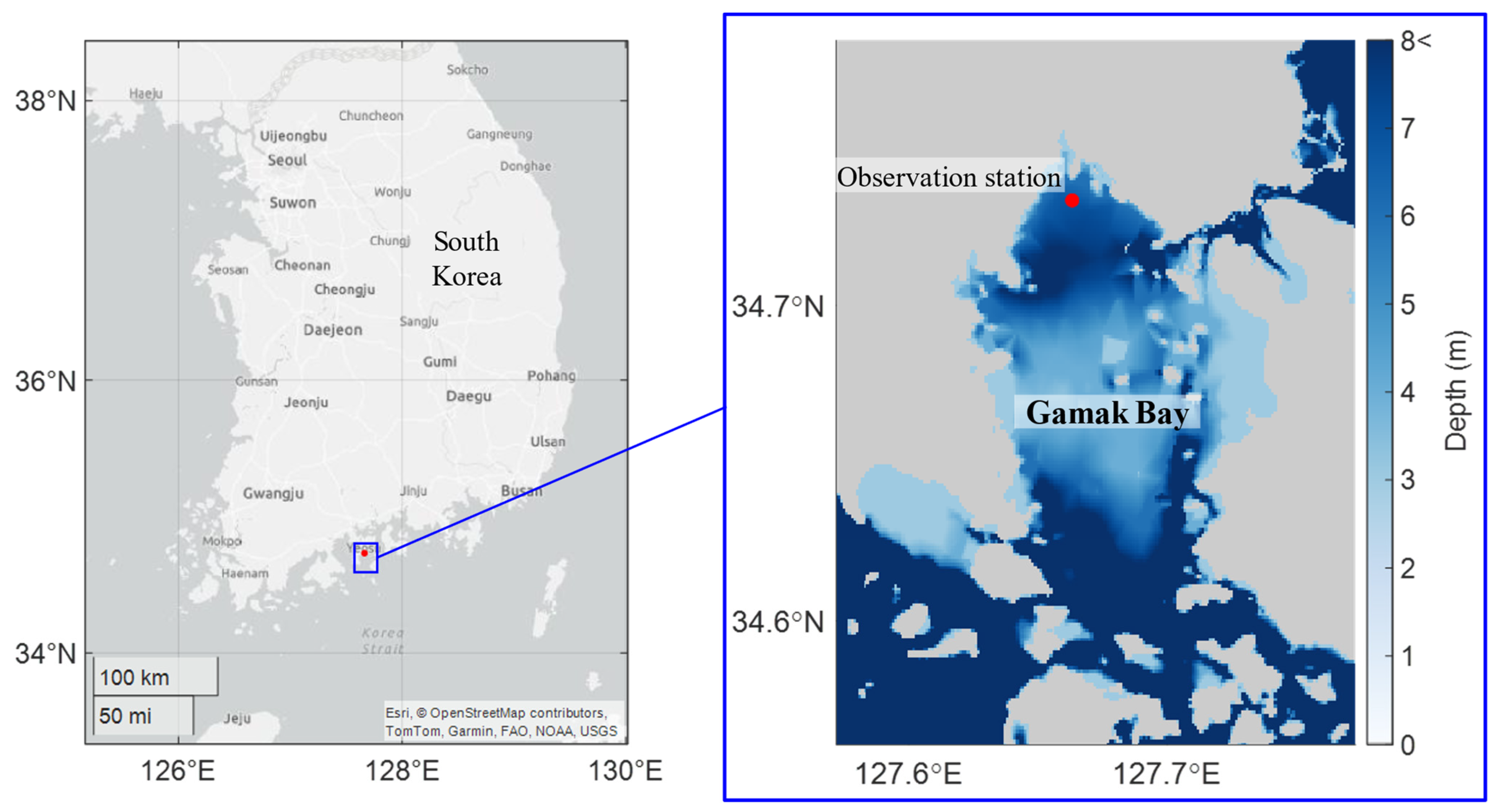
2. Materials and Methods

2.1. Data

Hourly observations of air temperature (AT), surface and bottom water temperature (WT), and surface and bottom DO concentration were conducted from May to November each year during the period 2017–2023 at a northern station in Gamak Bay (Figure 1). In the Korean seasonal context, May corresponds to spring, June through August to summer, and September through November to autumn. AT was measured using a Mini-C5A RS232 sensor (Veinasa, Chengdu, China), WT with a C4E digital sensor (AQUALABO, Champigny-sur-Marne, France), and DO concentration with an OPTOD sensor (AQUALABO, Champigny-sur-Marne, France). Missing segments in the AT records were filled using data from the Korea Meteorological Administration’s Yeosu observation station (34.7393° N, 127.7406° E) [20].

One of the objectives of this study was to compare the predictive performance of bottom DO concentrations with and without consideration of tide level. Gamak Bay is predominantly influenced by semidiurnal tides [21], with a tidal period of approximately 12.5 h. To prevent interpolation bias and minimize its influence on model performance, only continuous missing data of 12 h or less were filled using a spline interpolation.

Descriptive statistics for the dataset used in model training and validation are summarized in

Table 1. Descriptive statistics of the training data.

	Min	Max	Mean	Median	Standard Deviation	Missing Rate (%)
TL 1 (m)	−1.7	1.7	−0.1	0.0	0.8	0.0
AT 2 (°C)	3.1	36.2	21.5	22.0	5.1	0.0
Surface WT 3 (°C)	13.7	32.5	23.8	24.3	4.1	5.7
Bottom WT 3 (°C)	13.7	30.4	22.4	22.8	3.4	4.6
Surface DO 4 (mg/L)	0.0	19.8	8.3	8.3	2.0	9.0
Bottom DO 4 (mg/L)	0.0	12.9	4.1	4.3	3.0	5.7

Notes: ¹ tide level, ² air temperature, ³ water temperature, ⁴ dissolved oxygen.

. A total of 31,162 hourly records were available. Of these, data from 2017 to 2021 (n = 22,775; 73% of the total) were used for model training, data from 2022 (n = 4440; 14%) were used for validation, and data from 2023 (n = 3947; 13%) were used for model testing. The training dataset was standardized prior to model development by scaling each variable to have a mean of 0 and a standard deviation of 1.

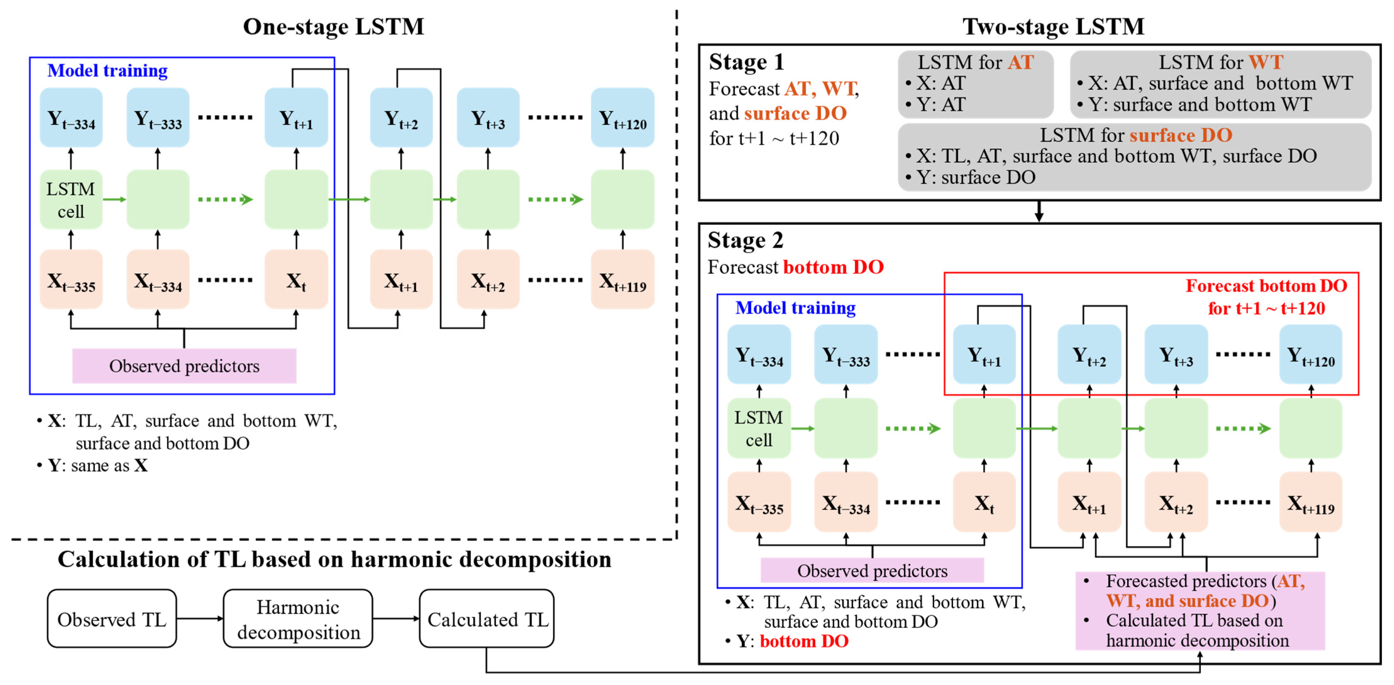
2.2. LSTM Architectures

Figure 2 illustrates the overall framework for forecasting bottom DO concentration. Two primary modeling strategies were adopted (one- and two-stage), each was tested with TL (WTL) and without TL (WoTL) as a predictor. In all cases, the target forecast horizon spanned from t + 1 to t + 120 (hour) and was updated on an hourly basis. Comparisons among these four models elucidate (1) the impact of tide level on model performance, and (2) whether a two-stage approach outperforms a single-stage approach in terms of forecast accuracy.

• One-stage without TL (Os-WoTL): A single LSTM model is trained to forecast all variables simultaneously. The predictor excludes TL.
• One-stage with TL (Os-WTL): Same as Os-WoTL, but with tide level included as an additional predictor.
• Two-stage without TL (Ts-WoTL): Stage 1 forecasts AT, WT, and surface DO; these predicted variables are then used as inputs in Stage 2 to forecast bottom DO.
• Two-stage with TL (Ts-WTL): Same as Ts-WoTL, except that the predictor set includes tide level calculated by harmonic decomposition.

2.3. LSTM Hyperparameters

The hyperparameters for all LSTM models were set as follows: one hidden LSTM layer, one dropout layer with a dropout rate of 50%, a sequence length of 336 h, 200 hidden nodes, a mini-batch size of 256, and the Adam optimizer. To ensure a fair comparison of model performance depending on the inclusion of tide level and the model architecture, all models were configured with the same hyperparameters. During training, overfitting was monitored using the validation dataset (observations from the year 2022), and training was terminated early when signs of overfitting were detected.

2.4. Model Evaluation

Model accuracy was evaluated based on three metrics: the root mean square error (RMSE), the coefficient of determination (R²), and the hypoxia prediction accuracy (AccH), all assessed across forecast lead times ranging from 1 to 120 h. AccH represents overall classification accuracy and is a widely accepted metric for binary classification tasks such as distinguishing hypoxia occurrence or non-occurrence (Equation (1)) [22].

$$\mathrm{A}\mathrm{c}\mathrm{c}\mathrm{H}={\displaystyle \frac{TP+TN}{n}}\times 100 (\%)$$

(1)

where $n$ is the number of observations. $TP$ refers to the number of cases in which both the observed and predicted DO concentrations are below the hypoxia threshold (3 mg/L), whereas $TN$ refers to the number of cases in which both observed and predicted values are equal to or above 3 mg/L.

2.5. Tide Level Calculation Based on Harmonic Decomposition

Tidal harmonic decomposition assumes that the tide level can be represented as the sum of multiple sinusoidal components corresponding to known astronomical frequencies [23]. Using standard harmonic decomposition (see Equation (2)), the four major tidal constituents (M₂, S₂, K₁, and O₁) were used to reconstruct the tide level. Harmonic constants and observed tide level data were obtained from the Korea Hydrographic and Oceanographic Agency (

Table 2. Harmonic constants of the four major tidal constituents in Gamak Bay.

Major Tidal Constituents	Amplitude (cm)	Phase Lag (°)	Period (h)
M2	101.2	253.9	12.4
S2	47.4	282.7	12.0
K1	20.2	190.7	23.9
O1	12.2	152.6	25.8

) [24].

$$\mathrm{T}\mathrm{L}=\sum _{i=1}^4{H}_i\cos \left({\displaystyle \frac{2\pi }{T_i}}t+{\varphi }_i\right)$$

(2)

where $i$ represents the four major constituents, $H$ is the amplitude, $T$ is the period, $\varphi$ is the phase lag, and $t$ is the time value.

Using the harmonic constants, tide levels were calculated and then compared with observed values to assess accuracy. The R² between the calculated and observed tide levels was 0.86, and RMSE was 0.31 m, indicating high reproducibility (Figure 3a). A time series comparison also demonstrated strong agreement between the two datasets (Figure 3b).

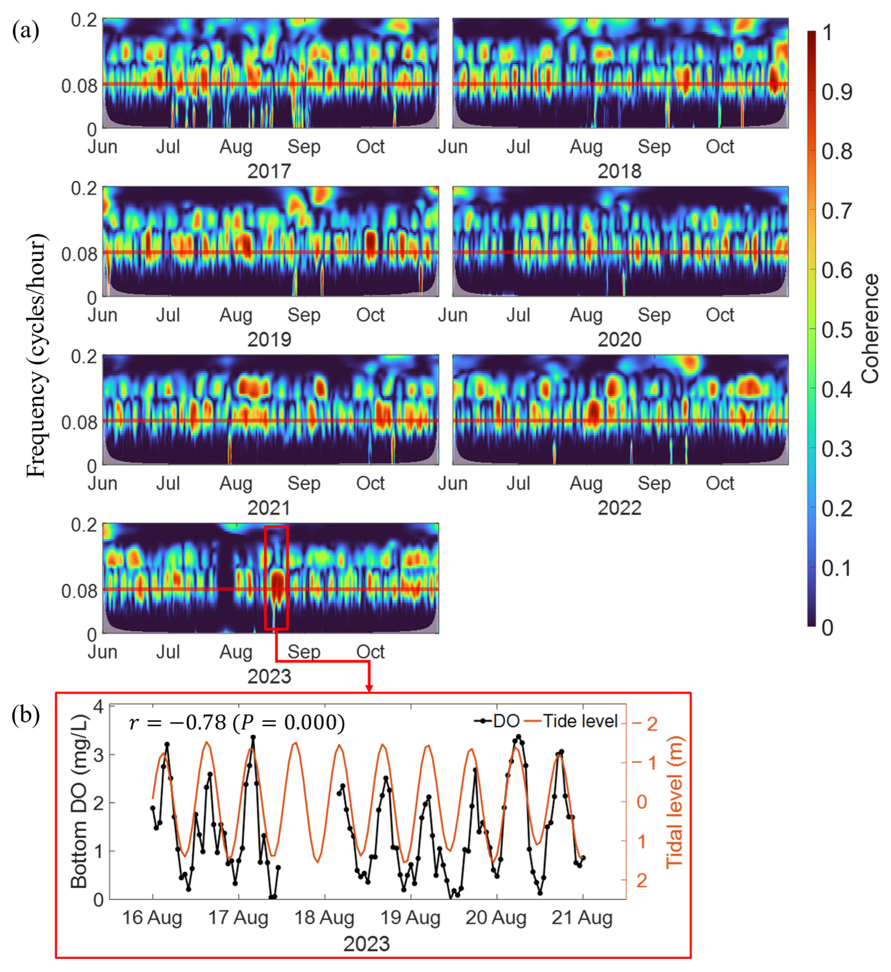
2.6. Wavelet Coherence Analysis

To investigate the time–frequency relationship between bottom DO concentration and tide level, wavelet coherence analysis was conducted. This function computes the magnitude-squared wavelet coherence, which quantifies the local correlation between two non-stationary time series across both time and frequency domains. The analysis was performed using the Morlet wavelet as the default mother wavelet [25].

$${\psi }_{s,\tau }\left(t\right)={\displaystyle \frac{1}{\sqrt{s}}}\psi \left({\displaystyle \frac{t-\tau }{s}}\right) \left(Morlet \psi \left(t\right)={\pi }^{-{\displaystyle \frac{1}{4}}}{e}^{i{\omega }_{0}t}{e}^{-{\displaystyle \frac{t^2}{2}}}\right)$$

(3)

$$W_x\left(s,\tau \right)={\int }_{-\infty }^{\infty }x\left(t\right){\psi }_{s,\tau }^{\ast }\left(t\right) dt, W_y\left(s,\tau \right)={\int }_{-\infty }^{\infty }y\left(t\right){\psi }_{s,\tau }^{\ast }\left(t\right) dt$$

(4)

$$\mathrm{W}\mathrm{a}\mathrm{v}\mathrm{e}\mathrm{l}\mathrm{e}\mathrm{t} \mathrm{c}\mathrm{o}\mathrm{h}\mathrm{e}\mathrm{r}\mathrm{e}\mathrm{n}\mathrm{c}\mathrm{e}={\displaystyle \frac{{\left|S\left\{s^{-1}{W}_x(s,\tau )W_y^{\ast }(s,\tau )\right\}\right|}^2}{S\left\{s^{-1}{\left|W_x(s,\tau )\right|}^2\right\} S\left\{s^{-1}{\left|W_y(s,\tau )\right|}^2\right\}}}$$

(5)

where * denotes the complex conjugate, S{·} is a two-dimensional Gaussian smoothing operator, s is the wavelet scale, τ is the time shift that slides the wavelet along the time axis, and x and y are the two input time-series being compared [26,27,28]. The wavelet coherence coefficient ranges from 0 (no correlation) to 1 (perfect local correlation). Coherence values above 0.5 are considered indicative of significant interactions between the two variables [28]. The resulting time-frequency coherence spectra enabled identification of dominant periodicities, such as semi-diurnal tidal signals, and their temporal synchronization with fluctuations in bottom DO concentration.

3. Results

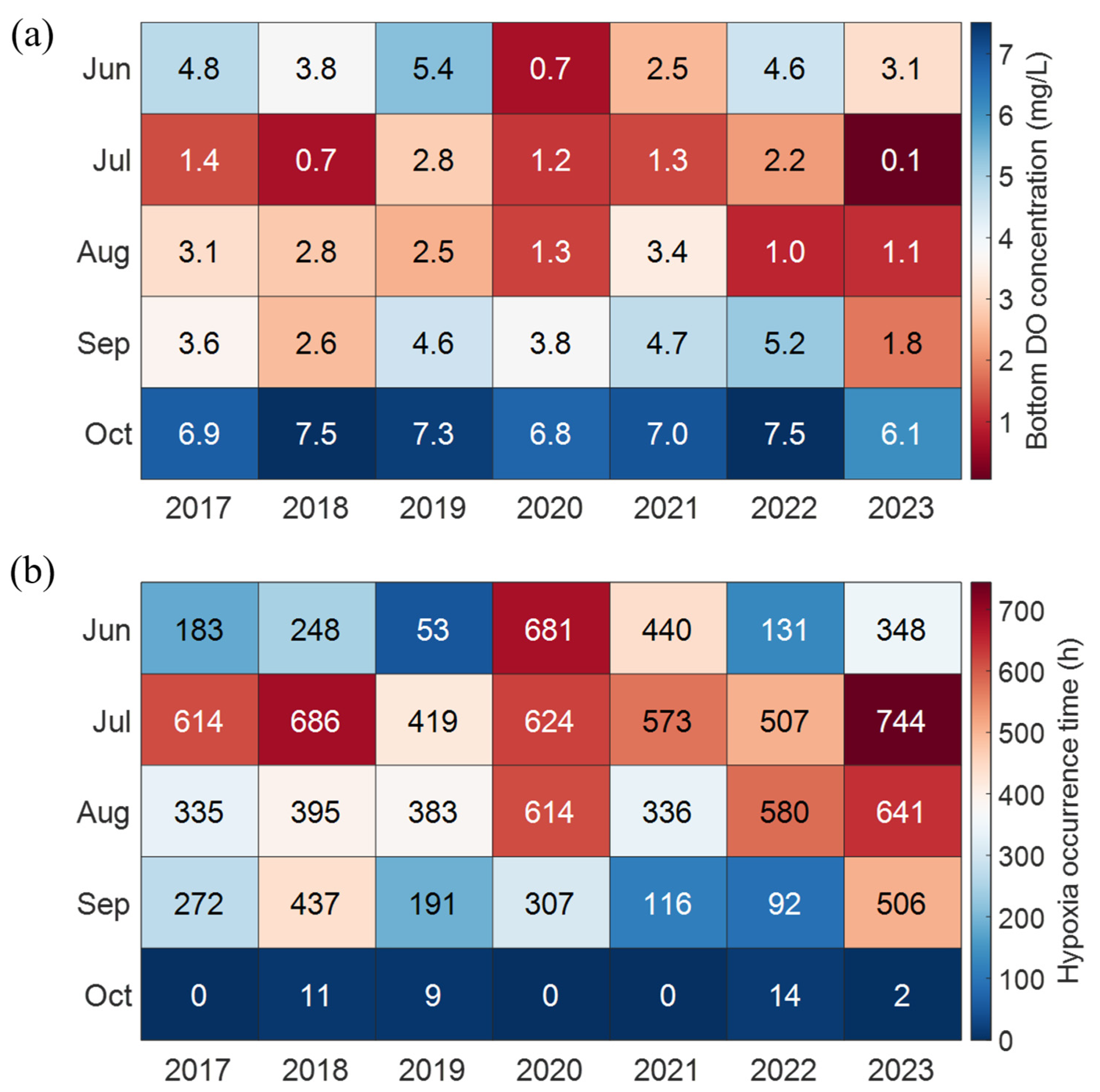
3.1. Occurrence of Hypoxia in Gamak Bay

The monthly average AT in the study area increased from 21.4 °C in June to 25.1 °C in July and 26.9 °C in August, then decreased to 22.8 °C in September and 17.4 °C in October (Figure 4a). The monthly average surface WT exhibited a similar seasonal pattern, rising from 23.8 °C in June to 28.5 °C in August, before declining to 20.9 °C in October (Figure 4b). The average WT difference between surface and bottom layers was 2.1–2.9 °C from June to August, indicating thermal stratification, which diminished in September (0.4 °C) and October (0.1 °C). Monthly average surface DO concentrations ranged from 7.7 to 8.8 mg/L, showing minimal seasonal variation (Figure 4c). In contrast, average bottom DO concentrations decreased from 3.5 mg/L in June to 1.4 mg/L in July and 2.2 mg/L in August, before recovering to 3.6 mg/L in September and 7.0 mg/L in October. Hypoxic events were frequent in July and August, coinciding with higher WT and stratification.

In July, the average bottom DO concentrations ranged from 0.1 to 2.8 mg/L across different years, consistently falling below the hypoxia threshold of 3 mg/L (Figure 5a). Notably, July 2023 recorded the lowest average bottom DO concentration at 0.1 mg/L, with hypoxic conditions persisting for 744 h, indicating continuous hypoxia throughout the month (Figure 5b). In August 2023, hypoxic conditions lasted for 641 h, the longest duration compared to other years. These frequent hypoxic events in 2023 are attributed to the unique bathymetry and stratification of Gamak Bay. The northern inner bay, where the observation station is located, features a concave seabed topography that reduces water exchange, making it susceptible to hypoxia during summer stratification [8]. In July and August 2023, the WT difference between surface and bottom layers was 3.4 °C, which is 0.8 °C higher than the 2017–2022 average of 2.6 °C, indicating stronger stratification in 2023. Thus, the combination of intensified stratification and the bay’s concave seabed likely led to the severe hypoxic conditions observed during these months. However, because tide-induced changes in water depth, in addition to stratification, also affect vertical mixing and can contribute to the formation of coastal hypoxia, tidal influences must likewise be considered.

3.2. Correlation Between Bottom DO Concentration and Tide Level

Figure 6a presents wavelet coherence analysis between bottom DO concentrations and tide levels during 2017–2023. The color-coded values (0–1) represent coherence, quantifying the degree of synchronization between the two variables at specific frequency bands. Typically, coherence values above 0.5 suggest a significant interrelationship. The analysis revealed high coherence at a period of approximately 12.5 h (0.08 cycles/hour), indicating a close synchronization between bottom DO concentrations and tide levels at this frequency. This finding is noteworthy as Gamak Bay is predominantly influenced by semidiurnal tides, with the M2 constituent (12.4-h period) being the most dominant among the four major tidal constituents. The recurring detection of this synchronization during summer months across multiple years suggests that tidal fluctuations play a crucial role in influencing bottom oxygen conditions in coastal environments. Specifically, during 16–21 August 2023, when coherence between bottom DO concentration and tide level was strongest, a significant negative correlation was observed (r = −0.78, p < 0.05; Figure 6b). These results demonstrate that semidiurnal tidal forcing is a persistent and dominant driver of bottom-water oxygen dynamics in Gamak Bay. Consequently, any forecasting framework that aims to predict hypoxia in this system must explicitly account for tide-related variability. To evaluate this hypothesis, we incorporate tidal variability into the prediction models discussed in Section 3.3.

3.3. Comparison of Model Accuracy

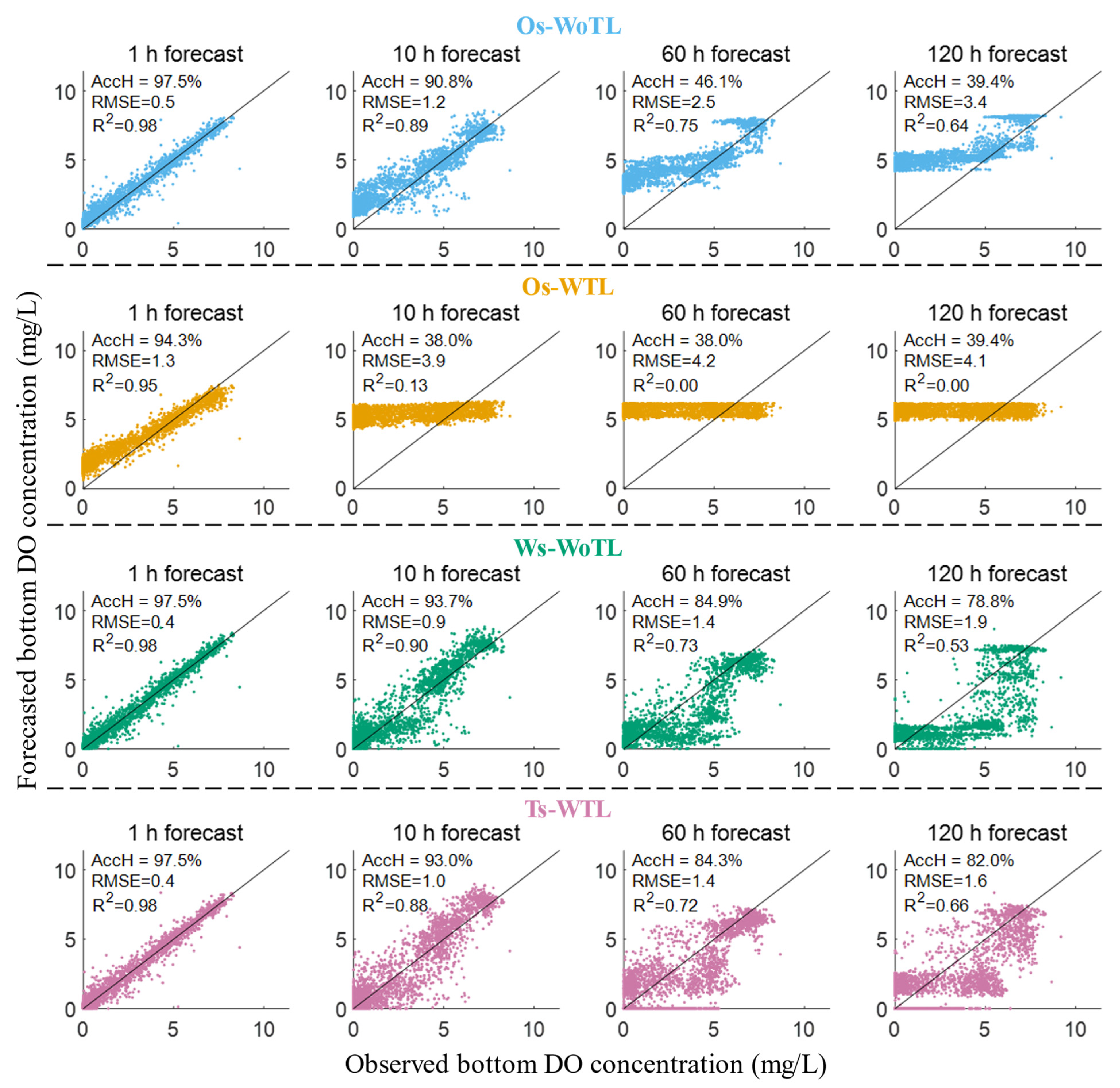
3.3.1. One- vs. Two-Stage LSTM Models with and Without Tide Level

The Os-WTL model achieved high short-term prediction accuracy, with a 1 h forecast RMSE of 1.3 mg/L and R² of 0.95 (Figure 7). However, its performance declined sharply as the forecast horizon increased, with a 10 h forecast RMSE of 3.9 mg/L and R² of only 0.13. In contrast, the Os-WoTL model, which excluded tide level as a predictor, showed relatively higher accuracy at the 10 h forecast horizon, with an RMSE of 1.2 mg/L and R² of 0.89. These results suggest that, under a one-stage model architecture, incorporating tide level may lead to inaccurate representations, and in such cases, excluding tide level may be more effective. However, as demonstrated in the previous analysis (Section 3.2), bottom DO concentrations in coastal waters are strongly influenced by tidal fluctuations. Without accurately accounting for tidal effects, reliable long-term forecasts of hypoxia become infeasible. Indeed, the Os-WoTL model, which excluded tide level, showed poor long-term performance, with a 120 h forecast AccH of only 39.4%, RMSE of 3.4 mg/L, and R² of 0.64, failing to predict hypoxic events altogether.

The two-stage LSTM models demonstrated relatively better long-term prediction performance compared to their one-stage counterparts. The Ts-WoTL model, which excluded tide level, yielded a 120-h forecast RMSE of 1.9 mg/L—1.5 mg/L lower than Os-WoTL—and an AccH of 78.8%, which was 39.4% higher. Notably, the Ts-WTL model, which effectively incorporated tide level through harmonic decomposition and a two-stage architecture, achieved the best long-term prediction performance among all models, with a 120-h AccH of 82.0%, RMSE of 1.6 mg/L, and R² of 0.66. These findings indicate that, for accurate forecasting of coastal hypoxia, it is essential to incorporate reliable tidal information into the model, which can be effectively achieved through harmonic decomposition and a two-stage modeling approach.

Figure 8 presents time series comparisons between observed and forecasted bottom DO concentrations over 1–120 h prediction horizons, predicted at specific time points during the test period (2023). These cases were chosen to illustrate model performance across varying seasonal and hypoxic conditions.

During June 23–27, bottom DO concentrations gradually decreased and then exhibited a sudden increase on June 27. Although the two-stage models (Ts-WoTL and Ts-WTL) successfully captured the initial declining trend, they failed to reproduce the abrupt rise on the 27th. This highlights a fundamental limitation of long-term forecasting in accurately capturing sudden fluctuations in DO levels. Consequently, the average RMSE for 1–120 h forecasts in June (1.9 mg/L) was higher than in other months, including July (0.1 mg/L), August (1.2 mg/L), September (1.6 mg/L), and October (1.3 mg/L). This relatively large forecasting error in June is likely due to the high variability in DO concentrations during this month, with a standard deviation of 2.3 mg/L; this is approximately 0.3–0.8 mg/L higher than in other seasons.

In July, when persistent hypoxic conditions were observed, the two-stage models were able to successfully predict sustained low DO levels, whereas the one-stage models (Os-WoTL and Os-WTL) failed to do so, resulting in substantial overestimation.

During the period of August 16–20, DO concentrations fluctuated in response to tidal variations. Among all models, only the Ts-WTL model was able to reproduce the observed tidal-driven oscillations, indicating the importance of explicitly incorporating tide level through a two-stage approach.

In October, when DO variability was relatively low, all models except Os-WTL achieved high predictive accuracy, suggesting that model performance improves under stable conditions, and that inclusion of tide level in a one-stage architecture may lead to substantial error.

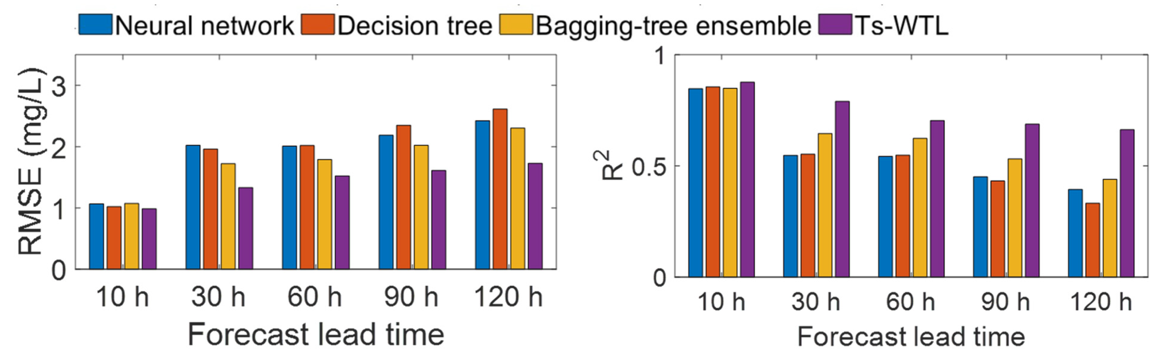
3.3.2. Benchmarking Ts-WTL Against Other Machine-Learning Models

To further evaluate the performance of the proposed Ts-WTL model, we compared it with three widely used machine-learning models: neural network, decision tree, and bagging-tree ensemble. All benchmark models were independently trained for each forecast lead time (10, 30, 60, 90, and 120 h), and the hyperparameters were optimized using Bayesian optimization.

As shown in Figure 9, the Ts-WTL model consistently outperformed all benchmark models across all lead times. In terms of RMSE, Ts-WTL yielded the lowest prediction error at each forecast lead time, with values ranging from 0.70 mg/L at 10 h to 1.30 mg/L at 120 h. In contrast, the RMSEs for the benchmark models were generally higher, with the largest gap observed at 120 h, where the decision tree model recorded 1.97 mg/L.

Similar trends were observed for the R² values. While all models achieved high R² values at short lead times (10 h), their performance declined significantly as the forecast lead time increased. The Ts-WTL model maintained the highest R² values throughout, reaching 0.66 at 120 h, compared to 0.39, 0.33, and 0.44 for neural network, decision tree, and bagging-tree ensemble, respectively.

These results demonstrate that the two-stage LSTM framework, especially when coupled with tide-level input, is better suited for long-term bottom DO forecasting than conventional machine-learning models. Notably, the Ts-WTL model exhibited a slower degradation in performance with increasing lead time, highlighting its robustness for multi-day hypoxia early warning.

4. Discussion

4.1. Causal Relationship Between Bottom DO Concentration and Environmental Variables

Table 3. Correlation coefficients and feature importance between bottom dissolved oxygen (DO) concentration and environmental variables. WT: water temperature, AT: air temperature.

	Surface DO	Tide Level	Surface WT	Bottom WT	AT
Correlation coefficient	0.09	−0.07	−0.71	−0.55	−0.67
Feature importance	19.90	8.79	17.55	18.85	6.53

summarizes the correlation coefficients and the feature importance values between bottom DO concentration and environmental variables (surface DO, tide level, surface and bottom WT, and AT). The feature importance values were derived from a random forest model that used five environmental variables as predictors. A higher feature importance indicates a greater contribution to DO prediction.

Surface and bottom WT both showed significant negative correlations with bottom DO (p < 0.05). Surface WT had the strongest correlation (r = −0.71): warmer surface water lowers oxygen solubility and strengthens stratification, which in turn suppresses vertical mixing and limits oxygen delivery to the seabed [29]. Bottom WT was also inversely related to bottom DO (r = −0.55). Rising bottom WT accelerates respiration and microbial decomposition, thereby consuming oxygen [30]; however, it can also weaken stratification, partially offsetting this effect, which explains the weaker correlation compared with surface WT.

AT displayed a similarly strong negative correlation (r = −0.67, p < 0.05). This link is likely indirect, arising from AT control of surface water warming. Consistent with that interpretation, AT had the lowest feature importance of 6.53.

Surface DO (r = 0.09) and tide level (r = −0.07) showed weak correlations with bottom DO. Their influence is mediated by vertical mixing dynamics that a single linear coefficient cannot capture. In fact, the bottom DO–tide relationship is inherently nonlinear [31]. At the study site, the water column averages ~8 m but fluctuates from 5.8 m at low tide to 9.9 m at high tide. During July–August, surface DO averaged 8.3 mg/L, whereas bottom DO averaged just 1.8 mg/L—a steep vertical gradient. High tide deepens the water column, suppresses mixing, and restricts oxygen-rich surface water from reaching the seabed, so bottom DO decreases. Low tide makes the column shallow, enhances mixing, and temporarily boosts bottom DO. Repetition of this cycle generates the observed significant negative correlation (Figure 6b). A similar tide-driven DO pattern has been reported for Fukuyama Inner Bay in Japan [31]. These findings underline the importance of incorporating tide level into hypoxia forecasts for tide-dominated, shallow coastal waters.

When these mixing processes are modelled explicitly—here, via a multivariate random-forest—the feature importances of surface DO (19.90) and tide level (8.79) rise well above that of AT (6.53). This confirms that, although their simple correlations are modest, both variables exert a substantial, nonlinear control on bottom-water oxygen dynamics.

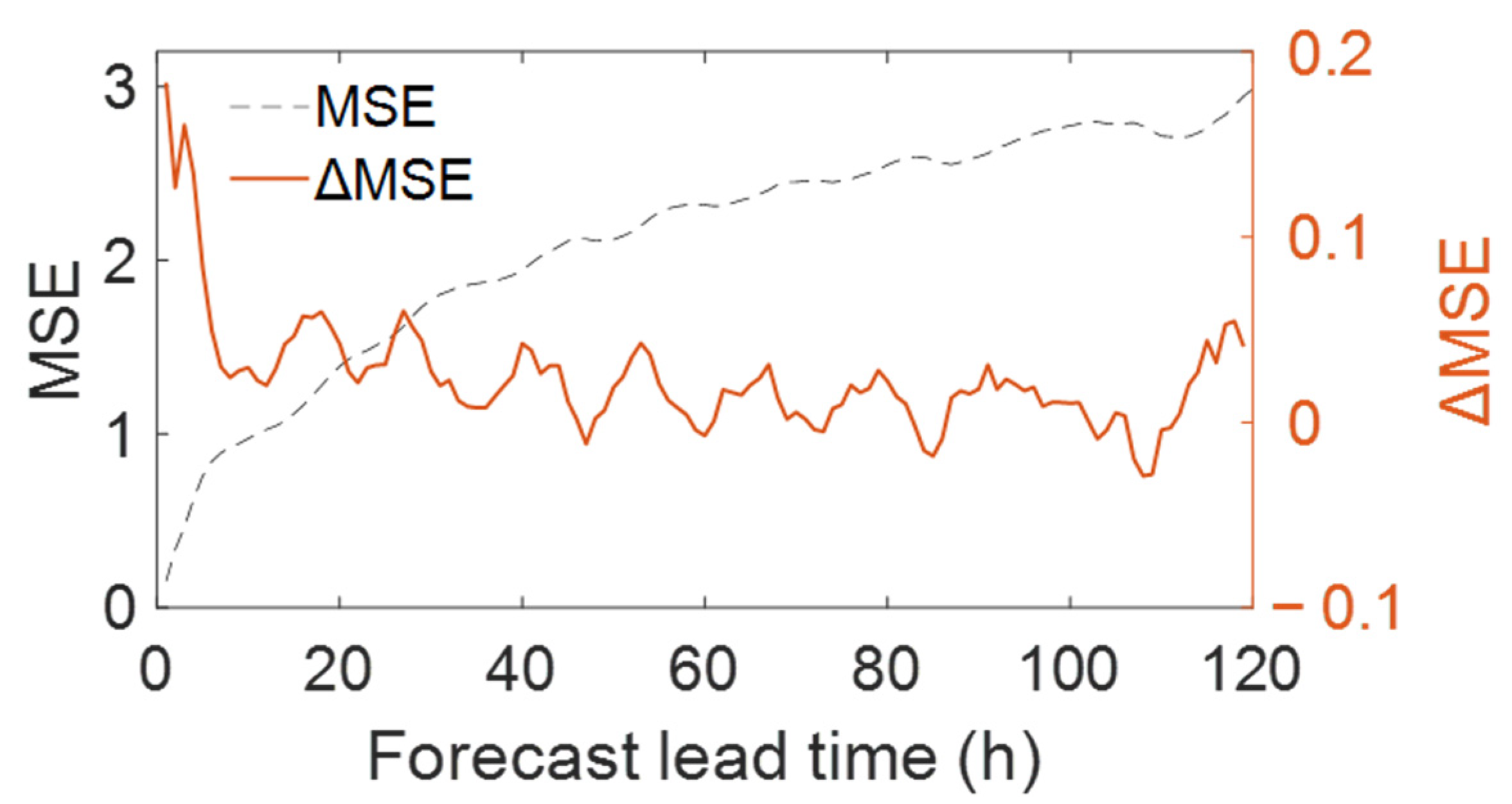
4.2. Considerations for Determining the Forecasting Horizon for Hypoxia

An important consideration in forecasting bottom hypoxia is determining how far into the future the model should aim to forecast its onset. For instance, a 1 h forecast provides insufficient lead time for meaningful mitigation or response measures. Therefore, the forecasting horizon must be long enough to enable timely decision-making for environmental management and resource protection.

One of the key factors in determining the appropriate forecasting horizon is the sensitivity of marine organisms to hypoxic conditions. A widely used biological indicator of such sensitivity is the LT50 (lethal time 50), which refers to the exposure duration at which 50% of the individuals in a population are expected to die under hypoxic conditions. According to the study by Vaquer-Sunyer and Duarte [32], which examined LT50 values for 206 marine species, the average LT50 under hypoxic conditions was 116.7 h. This implies that if a model can successfully forecast hypoxia 120 h in advance, a total response window of approximately 236.7 h (120 h + 116.7 h) can be secured. However, LT50 values vary considerably depending on species. For example, the average LT50 for 39 fish species was 59.9 h, and the 90th percentile (most sensitive 10% species) was as short as 0.9 h. Therefore, the forecasting horizon should be determined based on the dominant species in the target area and the hypoxia response capacity of the local government.

The reliability of model predictions is another critical consideration. In general, prediction accuracy tends to decline as the forecasting horizon increases. In this study, the Ts-WTL model showed an R² of 0.88 for a 10 h forecast, which dropped to 0.66 for a 120 h forecast. Thus, the forecasting horizon should be set based on the level of predictive accuracy required for the intended application. To quantify this accuracy decay, we plotted the mean-squared error (MSE) and its first difference (ΔMSE) across lead times (Figure 10). The ΔMSE curve remains close to zero up to ~110 h, indicating a roughly linear error growth. Beyond that point it rises sharply, signifying an inflection at which forecast performance deteriorates rapidly. We therefore adopted 120 h as the practical upper limit of the current model’s forecasting horizon.

In addition, factors such as the rate of hypoxia development and duration, the temporal resolution of observational data (e.g., hourly vs. daily), institutional thresholds, and model training costs must also be comprehensively considered when determining an appropriate forecasting horizon.

4.3. Future Considerations for Improving Model Accuracy

4.3.1. Hypoxia Characteristics in Gamak Bay

In this study, only a minimal set of predictor variables was considered in order to isolate and evaluate the influence of tide level on bottom DO concentration forecasts. However, future model development should incorporate additional features that more comprehensively reflect the hypoxia-generating characteristics specific to the study area.

Gamak Bay exhibits several distinct features that contribute to hypoxia formation. While the central region of the bay has a relatively shallow depth of approximately 4 m, the northern inner bay where the observation station is located is deeper, ranging from 7 to 9 m, and forms a concave basin-like topography (Figure 1). Due to this topography, the northern inner bay experiences limited water exchange, which—combined with stratification and heavy land-based pollutant loading during the summer—leads to frequent hypoxic events [8]. In addition, during hypoxic periods in Gamak Bay, the oxygen penetration depth in bottom sediments was shallow, and bottom DO concentrations were negatively correlated with nutrients [6]. Previous studies have also shown that the timing and duration of hypoxia events along the Korean coast are closely linked to extreme rainfall events associated with climate change [33].

Reflecting these localized hypoxia-generating features of Gamak Bay in future model development may lead to improved predictive performance.

4.3.2. Phase Classification of Bottom DO Concentration

In temperate coastal regions, bottom DO concentrations typically follow a seasonal progression that can be classified into three phases: Oversaturation, Depletion, and Stable [31]. The Oversaturation phase, observed during spring to early summer, is characterized by high variability in DO levels. During the summer, as stratification intensifies and terrestrial nutrient input increases, the Depletion phase emerges, marked by prolonged hypoxic conditions. In autumn, the system transitions into the Stable phase, where hypoxia dissipates and DO variability decreases.

These phase distinctions are also evident in Gamak Bay. For instance, time series data of bottom DO concentrations in 2023 (Figure 4c) showed that during spring to early summer (May–June), the standard deviation of bottom DO was 1.7 mg/L—higher than in summer (1.2 mg/L in July–August) and autumn (1.0 mg/L in October–November). The average bottom DO concentration during summer was only 0.6 mg/L, significantly lower than in spring–early summer (3.1 mg/L) and autumn (6.1 mg/L), indicating prolonged hypoxic conditions. In autumn, hypoxia was resolved, and DO concentrations stabilized.

Given that bottom DO exhibits clear seasonal dynamics, future model improvements may benefit from incorporating phase classification, either as an additional input variable or by training separate models for each phase. This phase-aware modeling approach could allow the network to better capture phase-specific dynamics, especially during the transitions into hypoxia, thereby enhancing predictive performance.

4.3.3. Hyperparameter Optimization

In this study, all models were implemented using identical hyperparameter settings to ensure a fair and quantitative comparison of the effect of tide level on DO forecasting accuracy. While this configuration allowed for controlled evaluation across model architectures, it is expected that further improvements in predictive performance can be achieved through hyperparameter optimization in future research.

4.4. Real-World Management Implication

The proposed forecasting framework has direct applications for real-time coastal management. For instance, predicting bottom hypoxia with a lead time of 3–5 days enables aquaculture facility managers to implement proactive measures, such as temporary harvesting, adjusting feeding rates, or deploying oxygenation systems to reduce fish mortality. Local authorities can also use the forecast information to issue public advisories, regulate effluent discharge during vulnerable periods, or reallocate monitoring resources to areas at higher risk of hypoxia. As the forecasting model operates on an hourly timescale, it is well-suited for integration into automated early warning systems, especially in coastal bays like Gamak Bay, where hypoxia events evolve rapidly. Such applications align with ongoing efforts in Korea’s coastal zone management policies to incorporate predictive tools for environmental resilience.

5. Conclusions

This study developed and evaluated a novel two-stage LSTM modeling framework for forecasting bottom DO concentrations in a semi-enclosed coastal system. By systematically assessing the effects of tide level and model architecture, we demonstrated the following key findings:

• Tide level, calculated using harmonic decomposition, significantly improved the long-term prediction of bottom DO concentration.
• The two-stage LSTM approach, which separates the prediction of intermediate environmental variables from the final DO forecast, outperformed conventional one-stage models in accuracy and hypoxia detection capability.
• The Ts-WTL model, which integrates tidal information into the two-stage framework, yielded the best overall performance, with a 120 h forecast RMSE of 1.6 mg/L and AccH (hypoxia prediction accuracy) of 82.0%.
• In benchmark comparisons with neural networks, decision trees, and bagging-tree ensemble, the proposed Ts-WTL approach consistently outperformed all alternatives.

Future research should explore incorporating additional predictors reflecting regional hypoxia mechanisms, implementing phase-aware modeling strategies, and conducting hyperparameter optimization to further enhance model performance. The modeling framework presented here offers a promising approach for improving early warning systems and adaptive management of coastal hypoxia.

References

1. Diaz, R.J.; Rosenberg, R. Spreading dead zones and consequences for marine ecosystems. Science 2008, 321, 926–929. [Google Scholar] [CrossRef]
2. Conley, D.J.; Carstensen, J.; Ærtebjerg, G.; Christensen, P.B.; Dalsgaard, T.; Hansen, J.L.; Josefson, A.B. Long-term changes and impacts of hypoxia in Danish coastal waters. Ecol. Appl. 2007, 17, S165–S184. [Google Scholar] [CrossRef]
3. Rabalais, N.N.; Turner, R.E.; Wiseman, W.J., Jr. Gulf of Mexico hypoxia, aka “The dead zone”. Annu. Rev. Ecol. Syst. 2002, 33, 235–263. [Google Scholar] [CrossRef]
4. Kim, H.; Franco, A.C.; Sumaila, U.R. A selected review of impacts of ocean deoxygenation on fish and fisheries. Fishes 2023, 8, 316. [Google Scholar] [CrossRef]
5. Wang, Z.; Pu, D.; Zheng, J.; Li, P.; Lü, H.; Wei, X.; Li, M.; Li, D.; Gao, L. Hypoxia-induced physiological responses in fish: From organism to tissue to molecular levels. Ecotoxicol. Environ. Saf. 2023, 267, 115609. [Google Scholar] [CrossRef]
6. Jeong, H.; Choi, S.; Cho, H. Characteristics of Hypoxic Water Mass Occurrence in the Northwestern Gamak Bay, Korea, 2017. J. Korean Soc. Mar. Environ. Saf. 2021, 27, 708–720. [Google Scholar] [CrossRef]
7. Seo, J.; Park, S.; Lee, J.; Choi, J. Structural changes in macrozoobenthic communities due to summer hypoxia in Gamak Bay, Korea. Ocean. Sci. J. 2012, 47, 27–40. [Google Scholar] [CrossRef]
8. Kim, J.; Park, J.; Jung, C.; Choi, W.; Lee, W.; Lee, Y. Physicochemical characteristics of seawater in Gamak Bay for a period of hypoxic water mass disappearance. J. Korean Soc. Mar. Environ. Saf. 2010, 16, 241–248. [Google Scholar]
9. Oh, H.; Lee, S.; Lee, W.; Jung, R.; Hong, S.; Kim, N.; Tilburg, C. Sustainability evaluation for shellfish production in Gamak Bay based on the systems ecology 1. EMERGY evaluation for shellfish production in Gamak Bay. J. Environ. Sci. Int. 2008, 17, 841–856. [Google Scholar] [CrossRef]
10. Ock, L.M.; Jin, P.S.; Soon, K.T. Influence of reclamation works on the marine environment in a semi-enclosed bay. J. Ocean Univ. China 2006, 5, 219–227. [Google Scholar] [CrossRef]
11. Regier, P.J.; Ward, N.D.; Myers-Pigg, A.N.; Grate, J.; Freeman, M.J.; Ghosh, R.N. Seasonal drivers of dissolved oxygen across a tidal creek–marsh interface revealed by machine learning. Limnol. Oceanogr. 2023, 68, 2359–2374. [Google Scholar] [CrossRef]
12. Long, J.; Lu, C.; Lei, Y.; Chen, Z.Y.; Wang, Y. Application of an improved LSTM model based on FECA and CEEMDAN VMD decomposition in water quality prediction. Sci. Rep. 2025, 15, 12847. [Google Scholar] [CrossRef] [PubMed]
13. Fang, P.; Wang, Y.; Zhao, Y.; Kang, J. Analysis of Prediction Confidence in Water Quality Forecasting Employing LSTM. Water 2025, 17, 1050. [Google Scholar] [CrossRef]
14. De Rango, A.; Furnari, L.; Cortale, F.; Senatore, A.; Mendicino, G. Wildfire Early Warning System Based on a Smart CO2 Sensors Network. Sensors 2025, 25, 2012. [Google Scholar] [CrossRef]
15. Guo, Q.; He, Z.; Wang, Z. Assessing the effectiveness of long short-term memory and artificial neural network in predicting daily ozone concentrations in Liaocheng City. Sci. Rep. 2025, 15, 6798. [Google Scholar] [CrossRef]
16. Li, J.; Meng, Z.; Zhang, J.; Chen, Y.; Yao, J.; Li, X.; Peng, Q.; Liu, X.; Cheng, C. Prediction of Seawater Intrusion Run-Up Distance Based on K-Means Clustering and ANN Model. J. Mar. Sci. Eng. 2025, 13, 377. [Google Scholar] [CrossRef]
17. Chen, X.; Shen, Z.; Li, Y.; Yang, Y. Tidal modulation of the hypoxia adjacent to the Yangtze Estuary in summer. Mar. Pollut. Bull. 2015, 100, 453–463. [Google Scholar] [CrossRef]
18. Tyler, R.M.; Brady, D.C.; Targett, T.E. Temporal and spatial dynamics of diel-cycling hypoxia in estuarine tributaries. Estuaries Coasts 2009, 32, 123–145. [Google Scholar] [CrossRef]
19. Lanoux, A.; Etcheber, H.; Schmidt, S.; Sottolichio, A.; Chabaud, G.; Richard, M.; Abril, G. Factors contributing to hypoxia in a highly turbid, macrotidal estuary (the Gironde, France). Environ. Sci. Process. Impacts 2013, 15, 585–595. [Google Scholar] [CrossRef]
20. Automated Synoptic Observing System. Available online: https://data.kma.go.kr/cmmn/main.do (accessed on 10 February 2023).
21. Lee, M.; Kim, B.; Kwon, Y.; Kim, J. Characteristics of the marine environment and algal blooms in Gamak Bay. Fish. Sci. 2009, 75, 401–411. [Google Scholar] [CrossRef]
22. Sokolova, M.; Lapalme, G. A systematic analysis of performance measures for classification tasks. Inf. Process. Manag. 2009, 45, 427–437. [Google Scholar] [CrossRef]
23. Doodson, A.T. The harmonic development of the tide-generating potential. Proc. R. Soc. Lond. Ser. A Contain. Pap. A Math. Phys. Character 1921, 100, 305–329. [Google Scholar]
24. Ocean Data in Grid Framework. Available online: http://www.khoa.go.kr/oceangrid/khoa/intro.do (accessed on 12 February 2023).
25. Morlet, J.; Arens, G.; Fourgeau, E.; Glard, D. Wave propagation and sampling theory—Part I: Complex signal and scattering in multilayered media. Geophysics 1982, 47, 203–221. [Google Scholar] [CrossRef]
26. Maraun, D.; Kurths, J. Cross wavelet analysis: Significance testing and pitfalls. Nonlinear Process. Geophys. 2004, 11, 505–514. [Google Scholar] [CrossRef]
27. Torrence, C.; Compo, G.P. A practical guide to wavelet analysis. Bull. Am. Meteorol. Soc. 1998, 79, 61–78. [Google Scholar] [CrossRef]
28. Grinsted, A.; Moore, J.C.; Jevrejeva, S. Application of the cross wavelet transform and wavelet coherence to geophysical time series. Nonlinear Process. Geophys. 2004, 11, 561–566. [Google Scholar] [CrossRef]
29. Wilson, P.C. Water quality notes: Dissolved oxygen: Sl313/ss525, 1/2010. EDIS 2010, 2010, 1–8. [Google Scholar] [CrossRef]
30. Robinson, C. Microbial respiration, the engine of ocean deoxygenation. Front. Mar. Sci. 2019, 5, 533. [Google Scholar] [CrossRef]
31. Park, S.; Kim, K.; Hibino, T.; Kim, K. Machine learning-based prediction of seasonal hypoxia in eutrophic estuary using capacitive potentiometric sensor. Mar. Environ. Res. 2024, 196, 106445. [Google Scholar] [CrossRef]
32. Vaquer-Sunyer, R.; Duarte, C.M. Thresholds of hypoxia for marine biodiversity. Proc. Natl. Acad. Sci. USA 2008, 105, 15452–15457. [Google Scholar] [CrossRef]
33. National Institute of Fisheries Science. 2024 Climate Change Impact and Research Report in the Fisheries Sector; National Institute of Fisheries Science: Busan, Republic of Korea, 2024. [Google Scholar]
Figure 1. Observation station and bathymetry of Gamak Bay.
Water 17 01622 g001
Figure 2. One-stage and two-stage LSTM modeling frameworks for bottom DO forecasting (AT: air temperature, WT: water temperature, TL: tide level).
Water 17 01622 g002
Figure 3. Comparison between observed and harmonically calculated tide levels: (a) scatter plot and (b) time series.
Water 17 01622 g003
Figure 4. Hourly time series of in situ observations in Gamak Bay from 2017 to 2023. (a) air temperature, (b) surface and bottom water temperature, and (c) surface and bottom DO concentrations are shown. The red dashed line in panel (c) indicates the threshold concentration of 3 mg/L for hypoxia.
Water 17 01622 g004
Figure 5. (a) Monthly mean bottom DO concentration and (b) total monthly hypoxia occurrence time based on hourly observations in Gamak Bay.
Water 17 01622 g005
Figure 6. (a) Time-frequency distribution of wavelet coherence between bottom DO concentration and tide level from 2017 to 2023 in Gamak Bay. The white translucent shading denotes the area outside the cone of influence (COI). (b) Time series comparison between bottom DO and tide level from 16 August to 21 August, 2023, which was the highest coherence period.
Water 17 01622 g006
Figure 7. Scatter plots comparing observed and forecasted bottom DO concentrations for 1 to 120 h forecasts generated by four LSTM models. The models include Os-WoTL (one-stage LSTM without tide level), Os-WTL (one-stage LSTM with tide level), Ts-WoTL (two-stage LSTM without tide level), and Ts-WTL (two-stage LSTM with tide level).
Water 17 01622 g007
Figure 8. Forecasts of hourly bottom DO concentration from four LSTM models over 1–120 h horizons at selected initialization times. Observed values (black line) and corresponding forecasts from each model are shown in each panel. For better visibility, markers are displayed every six hours.
Water 17 01622 g008
Figure 9. Comparison of bottom DO forecast performance (RMSE and R2) between the proposed two-stage LSTM model with tide level (Ts-WTL) and three benchmark machine-learning models (neural network, decision tree, and bagging-tree ensemble). For all benchmark models, a separate model was trained for each forecast lead time (i.e., the 10 h and 30 h models are independent), and hyperparameters were optimized using Bayesian optimization.
Water 17 01622 g009
Figure 10. Forecast performance decay of the Ts-WTL model. Dashed grey curve: lead-time dependence of mean-squared error (MSE). Solid orange curve: first difference (ΔMSE = MSEt − MSEt−1).
Water 17 01622 g010