A New Methodology to Estimate the Level of Water Stress (SDG 6.4.2) by Season and by Sub-Basin Avoiding the Double Counting of Water Resources

Abstract

While at the global level, water stress does not seem to present a serious threat to the sustainability of freshwater withdrawal and use, the situation appears much grimmer if a closer look is given to the status of the freshwater resources at basin and sub-basin levels. Unfortunately, such information is often not available to water managers and decision-makers, due both to the scarcity of sufficient data and also to the lack of methods capable of transforming the existing data into usable information. Hence, disaggregating water stress at basin and sub-basin levels is fundamental to provide a finer view of both its causes and effects, allowing the targeting of interventions at areas with high water stress and sectors with high water use. The spatial disaggregation of SDG indicator 6.4.2 by major river basin already implemented at a global scale showed the existence of a water stress belt running across the globe approximately between 10 and 45 degrees north, with a few other areas above and below it. The value of SDG indicator 6.4.2 at the country level is influenced by its size: the larger the country, the more the national average masks local variability. When the disaggregation is performed at sub-basin level, there is the possibility that the same amount of water is counted twice or even more (double counting), as it flows from one sub-basin to the neighbouring ones. Current water accounting methods do not allow this issue to be overcome. This causes an underestimation of water stress and an overestimation of the water resources available for human use in a given area. This paper presents a new methodology to assess SDG indicator 6.4.2 (water stress) seasonally and at the sub-basin level, addressing double counting by factoring in water demands between upstream and downstream sub-basins. This approach supports more informed water management. A corresponding plugin for the WEAP tool was developed, tested in the Senegal River basin countries, and is available online with a user manual in English, French, and Spanish.

1. Introduction

The rise in demand for water to meet the growing population, supply industries and sustain urban and rural populations has led to a growing scarcity of freshwater resources in many parts of the world [1,2]. In this context, agricultural ecosystems are facing increasing pressure because of competition from other water users, and few options remain globally to expand the agricultural area without significant environmental, social, and economic costs [3]. Water scarcity, defined as “an excess of water demand over available supply” [4], is a problem that can affect water security even in countries with ample water resources [5].

The 2030 Agenda for Sustainable Development was adopted in September 2015 by the United Nations. It consists of 17 Sustainable Development Goals (SDGs) with 169 targets, all interlinked in order to ensure an integrated approach towards more sustainable and resilient societies. Goal 6 on water and sanitation covers the entire water cycle in order to “ensure availability and sustainable management of water and sanitation for all” [6].

The aim of Target 6.4 is to “substantially increase water-use efficiency across all sectors and ensure sustainable withdrawals and supply of freshwater to address water scarcity and substantially reduce the number of people suffering from water scarcity” [6]. The SDG 6.4.2 indicator (level of water stress) is one of the two indicators identified to monitor this target, and it is defined as “the ratio between total freshwater withdrawn by all major sectors (TFWW) and total renewable freshwater resources (TRWR), after accounting for environmental flow requirements (EFR)” [6,7].

The purpose of this indicator is to show the degree to which freshwater resources are being exploited to meet a country’s water demand. It measures the country’s pressure on its freshwater resources and, therefore, the challenge to the sustainability of its water use. Low water stress indicates minimal potential impact on resource sustainability and on potential competition among users. High water stress, on the contrary, indicates substantial use of freshwater resources, with greater impacts on resource sustainability and the potential for conflict among users [7,8].

Globally, 18.6% of the available total renewable freshwater resources were being withdrawn in 2021, showing a general “no stress” condition of the globe. Nonetheless, this global value hides the higher values and the variability that exists at a finer scale [9]. The map of the indicator at the country level is in Figure 1a. Aggregating water stress values at global and regional levels masks significant disparities, stressing the need for disaggregation to better understand causes and impacts [10,11]. Such disaggregation facilitates policy- and decision-makers to target interventions more effectively, focusing on regions with high water stress and sectors with significant water use.

This document describes a methodology to disaggregate the SDG indicator 6.4.2 at basin and sub-basin (SB) level, including information on data and tools that can be used to implement the disaggregation. By applying this new methodology, countries will be able to analyse water stress and its components at the SB level, allowing them to understand the impact of projects such as irrigation schemes, new settlements, or industrial development on the availability of water resources, their impact on the neighbouring basins and the long-term sustainability of those projects in terms of water resources. In other words, this new approach supports more informed water management. A corresponding plugin for the WEAP tool was developed, tested in the Senegal River basin countries, and is available online with a user manual in English, French, and Spanish.

State of the Art and Bottlenecks

The SDG 6.4.2 indicator (level of water stress) expression is shown in Equation (1).

$$\mathrm{W}\mathrm{a}\mathrm{t}\mathrm{e}\mathrm{r} \mathrm{S}\mathrm{t}\mathrm{r}\mathrm{e}\mathrm{s}\mathrm{s}\left(\mathrm{\%}\right)={\displaystyle \frac{\mathrm{T}\mathrm{F}\mathrm{W}\mathrm{W}}{\mathrm{T}\mathrm{R}\mathrm{W}\mathrm{R}-\mathrm{E}\mathrm{F}\mathrm{R}}}\ast 100$$

(1)

At the global scale, the spatial disaggregation of indicator 6.4.2 by major river basin was implemented [8] using the national data on water withdrawals available in AQUASTAT [12] and mapping them on the FAO (FAO: Food and Agriculture Organisation of the United Nations) world map of the major hydrological basins [13]. The resulting map is shown in Figure 1b.

Overall, the outcome of the disaggregation by major basin shows the existence of a water stress belt running across the globe approximately between 10 and 45 degrees north, with a few other areas above and below it. Such analysis allows a better understanding of the global distribution of water stress, including the identification of those situations where country-level assessment may not provide sufficient information to support decision-making on the management of water resources at the regional- or sub-regional level. In this regard, by comparing Figure 1a with Figure 1b, it is possible to notice that countries that may appear on the ‘safe side’, such as the United States, China, India, and South Africa, but also Mexico, Peru and Chile, in fact include basins that are much more stressed than the national average. This confirms the importance of disaggregating water stress by hydrological units, going beyond the aggregated values calculated for the national SDG assessments.

The methodology applied to calculate water stress at the country scale and to disaggregate it to major river basins presented limitations due mainly to the availability of data, which was often outdated for both water resources and withdrawals [8]. Furthermore, two main issues were raised: The value of SDG indicator 6.4.2 depends on the size of the assessed area: The larger the country, the more the national average masks local variability; there are countries that are affected by “high water stress” despite the global average value (18.4 percent) showing the no-water-stress condition of the globe. Similarly, there are countries with a “low or medium water stress”, which indeed include basins that are critically water stressed (Figure 1a,b). For example, according to the data available in AQUASTAT [12], Peru and the United States have a water stress at the national level of 4.58% and 28.16%, respectively, while the disaggregation by major river basins reveals a water stress of about 70% in the Pacific coast of Peru and a water stress close to 80% in the Colorado river basin. When the unit used for the calculation of SDG indicator 6.4.2 has a hydrological connection with the neighbouring units, there is the possibility of counting twice or more the same amount of water (double counting) as it flows from one unit to the neighbouring ones. This happens when the total freshwater resource of a hydrological unit is computed by adding the vertical water inputs and outputs (e.g., precipitation, evapotranspiration) and the horizontal inflows and outflows of surface and groundwater [14,15]. Managing system interconnectivity is essential for ensuring the hydrological integrity of the system [16,17].

This paper proposes a new approach for computing a disaggregated value of SDG indicator 6.4.2 while avoiding the issue of double counting by establishing a linkage between water needs and availability among neighbouring hydrological units. This is performed by computing the total renewable freshwater resources by adding to the vertical water balance only that part of the inflow or outflow reserved to match the need of each hydrological unit. Although this new approach can be applied independently, a specific plug-in for the WEAP (Water Evaluation And Planning tool) is presented to apply the proposed methodology for the computation of the water stress at sub-basin level.

2. Methodology

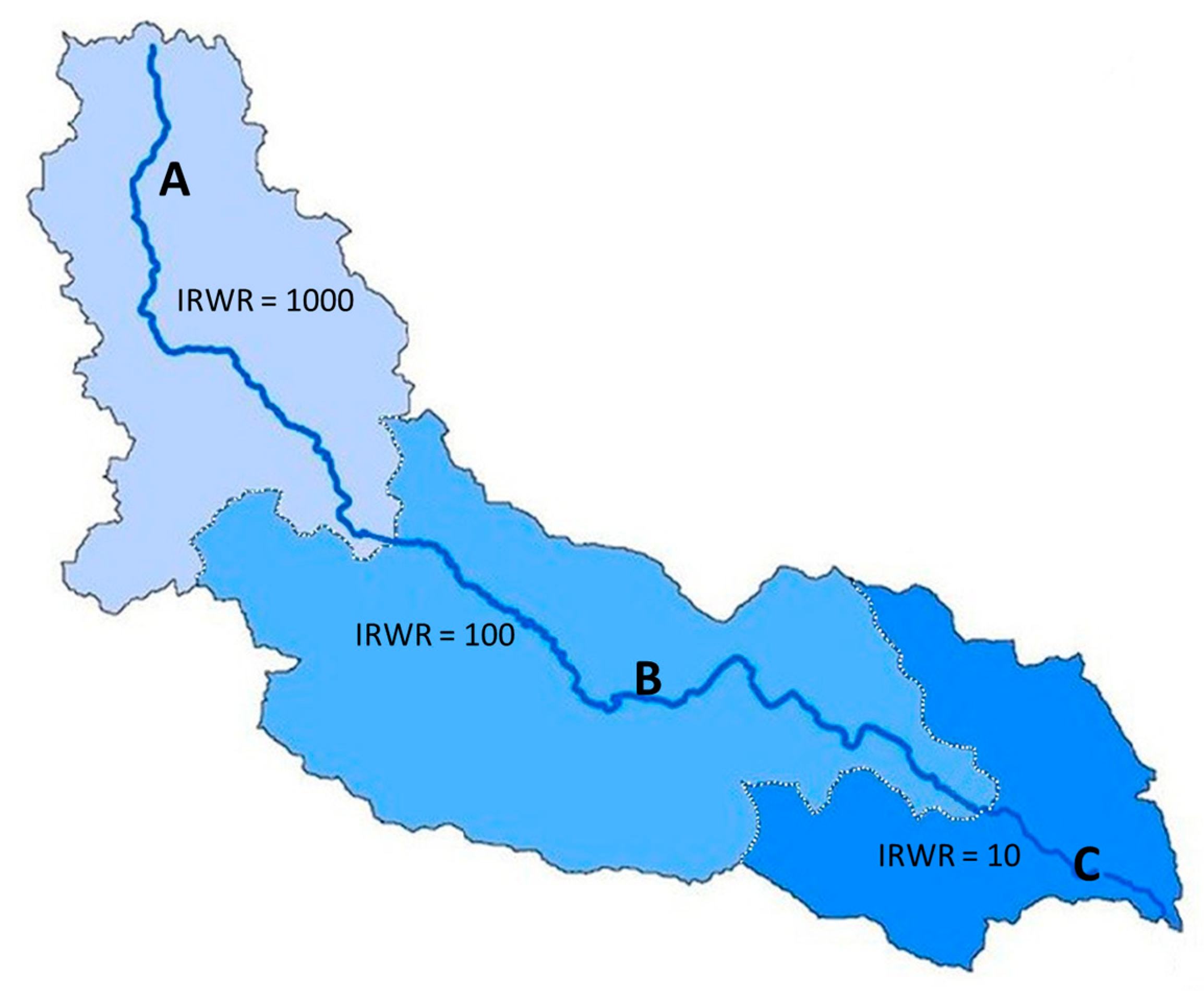
2.1. Internal Renewable Freshwater Resources

The new approach proposed in this document for calculating indicator 6.4.2 considers a hydrological unit for disaggregation. This facilitates the calculation of a water balance, because its application requires that the necessary data be available.

The law of water balance states that the inflows (input) to any hydrologic unit are equal to its outflows (outputs) plus change in storage during a time interval [18], as expressed in the following equation:

P(i) − ET(i) − R(i) − G(i) = ∆S [m³/year]

(2a)

where for the hydrologic unit i: P(i) is the precipitation, ET(i) includes the actual evapotranspiration of natural vegetation, the ET of agriculture under rainfed conditions and the evaporation from bare soil as well as from open water, wetlands and swamps, R(i) is the runoff or drainage, G(i) is the groundwater recharge and ∆S is the change in the soil water storage.

Water balance accounting may be very general or very detailed, depending on the hydrologic complexity, the scale and the purpose of the analysis. Under long-term, stationary conditions, changes in storage are considered negligible; therefore, the water balance equation for a generic hydrologic unit (i) becomes:

P(i) − ET(i) − R(i) − G(i) = 0 [m³/year]

(2b)

Under such stationary conditions, the internal renewable freshwater resources (IRWR) of a hydrological unit (i) can be defined as the total annual precipitation (P) minus the evapotranspiration (ET) (Equation (3a)). Alternatively, it can be defined as the sum of runoff or drainage (R) and the groundwater recharge (G) (Equation (3b)).

IRWR (i) = R(i) + G(i) [m³/year]

(3a)

IRWR (i) = P(i) − ET(i) [m³/year]

(3b)

If the hydrologic unit i has no connection with neighbouring hydrologic units, its IRWR and TRWR will coincide. But, if the selected unit is hydrologically connected with other units, its TRWR(i) will be defined as the sum of the IRWR and the external renewable freshwater resources (ERWR), as expressed by Equation (4):

TRWR(i) = IRWR(i) + ERWR(i) [m³/year]

(4)

As explained in the next paragraph, ERWR(i) can be positive or negative depending on whether it flows into or out of the unit. Its inclusion within the equations is critical because it represents the key to avoiding double counting of water resources.

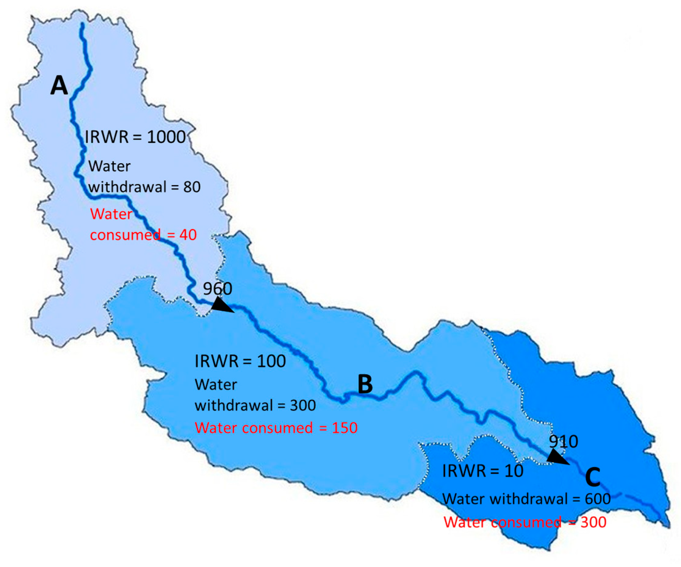
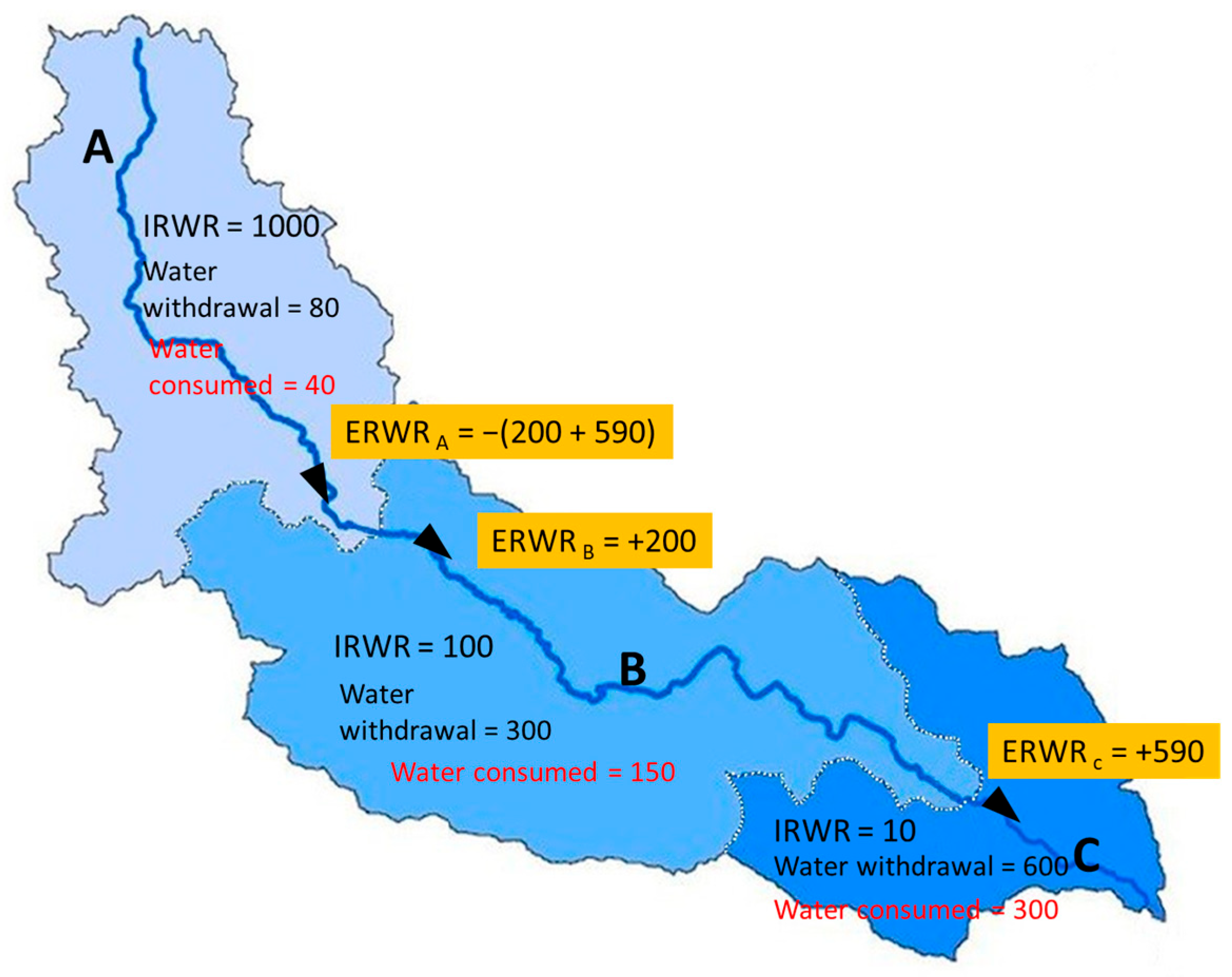
2.2. External Renewable Freshwater Resources

To explain the role of the ERWR, let us consider an example of a basin including three SBs: A (the head of the basin), B and C (Figure 2).

If the IRWR are, respectively, 1000, 100 and 10 Mm³, the TRWR of the entire river basin is:

TRWR = IRWR (A) + IRWR (B) + IRWR (C) = 1110 Mm³

To calculate the water exchanged between the SBs, it is necessary to know the water withdrawn and consumed in each SB. In this example it is assumed that the water is withdrawn for irrigation purposes only and the irrigation efficiency is about 50%; therefore, the freshwater consumed by irrigated agriculture in SB A, B and C is 40, 150 and 300 Mm³ respectively, so the water flowing from SB A to SB B is 960 Mm³, and from SB B to SB C is 910 Mm³ (Figure 3).

Consequently:

TRWR A = IRWR A + ERWR A = 1000 + 0 = 1000 Mm³

TRWR B = IRWR B + ERWR B = 100 + 960 = 1060 Mm³

TRWR C = IRWR C + ERWR C = 10 + 910 = 920 Mm³

By summing up the TRWR of the three SBs, it becomes evident that the freshwater accounted for the entire basin is much higher than 1110 Mm³. This occurs because the same amount of water was counted multiple times as it flowed from upstream to downstream. To avoid the double counting of the freshwater resources, it is necessary to modify the calculation of the ERWR.

Going back to Figure 3, we notice that while SB A can cover entirely its water demand, SB B and C have an important water deficit, as their IRWR are not sufficient to cover their water demands.

Internal water deficit SB B = 300 − 100 = 200 Mm³

Internal water deficit SB C = 600 − 10 = 590 Mm³

To avoid the double counting of the water resources, the ERWR of each SB is calculated accounting for the water allocated to cover the deficit downstream. In this way, the values of TRWR for each SB of Figure 3 become as follows (Figure 4):

TRWR A = IRWR A + ERWR A = 1000 − (200 + 590) = 210 Mm³

TRWR B = IRWR B + ERWR B = 100 + 200 = 300 Mm³

TRWR C = IRWR C + ERWR C = 10 + 590 = 600 Mm³

TRWR A + TRWR B + TRWR C = 1110 Mm³

From the example, it is evident that the ERWR accounted for in each SB can be positive (SB B and C) or negative (as in SB A), as it represents either the water amount allocated to fulfil the freshwater demand of that unit or that of its neighbouring units. In other words, this means that in each SB, the part of external water resources actually accounted for is only the amount allocated to fulfil the freshwater demand of that same unit or of its downstream neighbouring units. For this reason, despite SB A having the highest IRWR, its TRWR will be the lowest, as the majority of the water generated in SB A is allocated to SB B and C to cover their water deficit. This implies that the water accounted for in each hydrologic unit may be different from the water actually flowing.

2.3. Total Renewable Freshwater Resources

In order to calculate the level of water stress by hydrologic unit or SB, it is necessary to clarify all the terms involved in each variable of SDG indicator 6.4.2, defined by Equation (1), which can be rewritten as follows:

$$\mathrm{S}\mathrm{D}\mathrm{G} 6.4.2(\mathrm{i})={\displaystyle \frac{\mathrm{T}\mathrm{F}\mathrm{W}\mathrm{W}\left(\mathrm{i}\right)}{\mathrm{T}\mathrm{R}\mathrm{W}\mathrm{R}\left(\mathrm{i}\right)-\mathrm{E}\mathrm{F}\mathrm{R}\left(\mathrm{i}\right)}}\ast 100 [\%]$$

(5)

For an SB(i): TFWW(i) is the total freshwater withdrawals, TRWR(i) is the total renewable freshwater resources and EFR(i) is the environmental flow requirements to be covered in the SB(i). All the variables are expressed in [m³/year].

The TRWR for any given hydrologic unit (i) is equal to the sum of IRWR and the ERWR, the water exchanged with the neighbouring units (Equation (4)).

If the freshwater demand of a given hydrologic unit is fully met by its IRWR and there are still freshwater resources available, the water balance is positive, and the unit has an internal water surplus, which is calculated as follows:

$$\mathrm{i}\mathrm{n}\mathrm{t}\mathrm{e}\mathrm{r}\mathrm{n}\mathrm{a}\mathrm{l} \mathrm{w}\mathrm{a}\mathrm{t}\mathrm{e}\mathrm{r} \mathrm{s}\mathrm{u}\mathrm{r}\mathrm{p}\mathrm{l}\mathrm{u}\mathrm{s} \left(\mathrm{i}\right)=\mathrm{m}\mathrm{a}\mathrm{x} (0,\mathrm{I}\mathrm{R}\mathrm{W}\mathrm{R}(\mathrm{i}) - \mathrm{E}\mathrm{F}\mathrm{R}(\mathrm{i}) - \mathrm{T}\mathrm{F}\mathrm{W}\mathrm{W}(\mathrm{i}\left)\right) [{\mathrm{m}}^3/\mathrm{y}\mathrm{e}\mathrm{a}\mathrm{r}]$$

(6)

On the contrary, if the freshwater demand of the hydrologic unit is not fully covered by its IRWR, it will have an internal water deficit, which is calculated with the following equation:

$$\mathrm{i}\mathrm{n}\mathrm{t}\mathrm{e}\mathrm{r}\mathrm{n}\mathrm{a}\mathrm{l} \mathrm{w}\mathrm{a}\mathrm{t}\mathrm{e}\mathrm{r} \mathrm{d}\mathrm{e}\mathrm{f}\mathrm{i}\mathrm{c}\mathrm{i}\mathrm{t} \left(\mathrm{i}\right) = \mathrm{m}\mathrm{a}\mathrm{x} (0,\mathrm{T}\mathrm{F}\mathrm{W}\mathrm{W}(\mathrm{i}) + \mathrm{E}\mathrm{F}\mathrm{R}(\mathrm{i}) - \mathrm{I}\mathrm{R}\mathrm{W}\mathrm{R}(\mathrm{i}\left)\right) [{\mathrm{m}}^3/\mathrm{y}\mathrm{e}\mathrm{a}\mathrm{r}]$$

(7)

To eliminate the internal water deficit, there are two strategies that may be combined: reducing the freshwater demand or increasing the water supply. Reducing freshwater demand depends on management choices and the conditions of each hydrologic unit. Here, we analyse the aspects of increasing the water supply.

As explained in the previous section, the hydrologic units with a positive water balance are eligible to use their internal water surplus in full or in part to increase the water supply of the downstream neighbouring units with an internal water deficit.

Figure 5 shows an example of a river basin with 8 SBs, where some SBs experience an internal water surplus (blue) and the others have an internal water deficit (red).

Table 1. Direct connectivity matrix. It shows the position of each sub-basin (SB) in relation to its neighbouring sub-basins (SBs).

	SB1	SB2	SB3	SB4	SB5	SB6	SB7	SB8	Number of SBs Immediately Downstream
SB1	0	0	0	1	0	0	0	0	1
SB2	0	0	0	0	0	1	0	0	1
SB3	0	0	0	0	0	0	1	0	1
SB4	0	0	0	0	0	0	1	0	1
SB5	0	0	0	0	0	0	1	0	1
SB6	0	0	0	0	0	0	1	0	1
SB7	0	0	0	0	0	0	0	1	1
SB8	0	0	0	0	0	0	0	0	0
Number of SBs Immediately Upstream	0	0	0	1	0	1	4	1

is the direct connectivity matrix and shows the position of each SB relative to its neighbouring SBs.

Table 2. Indirect connectivity matrix showing the hydrological connection of each sub-basin (SB) with all the other sub-basins (SBs) of the river basin. Source: authors’ own elaboration.

	SB1	SB2	SB3	SB4	SB5	SB6	SB7	SB8	Total Number of SBs Downstream
SB1	0	0	0	1	0	0	1	1	3
SB2	0	0	0	0	0	1	1	1	3
SB3	0	0	0	0	0	0	1	1	2
SB4	0	0	0	0	0	0	1	1	2
SB5	0	0	0	0	0	0	1	1	2
SB6	0	0	0	0	0	0	1	1	2
SB7	0	0	0	0	0	0	0	1	1
SB8	0	0	0	0	0	0	0	0	0
Total Number of SBs Upstream	0	0	0	1	0	1	6	7

is the indirect connectivity matrix since it shows the relation of each SB with all the other SBs of the entire river basin.

The indirect connectivity matrix (Table 2) is key for computing the water stress at the SB level, as it is used to calculate the in-river water transferred from one SB to another, operating upon the hydrologic connections among SBs. For example, reading the table by rows, we see that SB1 can transfer water to SB4, SB7 and SB8, while SB2 can transfer water to SB6, SB7 and SB8. Similarly, if reading the table vertically, by column, we can see which SBs can be called upon to transfer water to the SB of that column. For example, SB6 can receive water only from SB2, while SB7 can receive water from SB1, SB2, SB3, SB4, SB5 and SB6 [19].

Table 3. Connectivity matrix showing the hydrological connection of each sub-basin (SB) with all the other sub-basins (SBs) of the river basin, considering their internal water deficit or surplus.

	SB1	SB2	SB3	SB4	SB5	SB6	SB7	SB8	Total Number of SBs Downstream to Reserve Water for (Downstream Reserve)
SB1	0	0	0	0	0	0	1	1	2
SB2	0	0	0	0	0	1	1	1	3
SB3	0	0	0	0	0	0	1	1	2
SB4	0	0	0	0	0	0	1	1	2
SB5	0	0	0	0	0	0	0	0	0
SB6	0	0	0	0	0	0	0	0	0
SB7	0	0	0	0	0	0	0	0	0
SB8	0	0	0	0	0	0	0	0	0
Total number of SBs upstream to request water from	0	0	0	0	0	1	4	4

shows the connectivity matrix, including the information related to the internal water deficit or surplus of the SBs. For example, SB1 can transfer water to SB4, SB7 and SB8, but since SB4 has no internal water deficit, SB1 will transfer water only to SB7 and SB8. If we read Table 3 vertically, SB7 can theoretically request water from SB1, SB2, SB3, SB4, SB5 and SB6, but since SB5 and SB6 have an internal water deficit, it can receive water only from SB1, SB2, SB3 and SB4. Meanwhile, SB6 can request water only from SB2, as such, SB2 will first cover the full internal water deficit of SB6. If any surplus water remains after this first transfer, then it can be transferred further downstream to SB7 and/or SB8.

The upstream request of a generic SB(i) depends on its internal water deficit and will be calculated considering the following expression:

$$\mathrm{U}\mathrm{p}\mathrm{s}\mathrm{t}\mathrm{r}\mathrm{e}\mathrm{a}\mathrm{m} \mathrm{r}\mathrm{e}\mathrm{q}.\left(\mathrm{i}\right) = \min \left(\mathrm{i}\mathrm{n}\mathrm{t}\mathrm{e}\mathrm{r}\mathrm{n}\mathrm{a}\mathrm{l} \mathrm{w}\mathrm{a}\mathrm{t}\mathrm{e}\mathrm{r} \mathrm{d}\mathrm{e}\mathrm{f}\mathrm{i}\mathrm{c}\mathrm{i}\mathrm{t}\left(\mathrm{i}\right),\mathrm{i}\mathrm{n}\mathrm{t}\mathrm{e}\mathrm{r}\mathrm{n}\mathrm{a}\mathrm{l} \mathrm{w}\mathrm{a}\mathrm{t}\mathrm{e}\mathrm{r} \mathrm{d}\mathrm{e}\mathrm{f}\mathrm{i}\mathrm{c}\mathrm{i}\mathrm{t}(\mathrm{i})\ast {\displaystyle \frac{{\sum }_{\mathrm{i}=1}^{\mathrm{n}}\mathrm{i}\mathrm{n}\mathrm{t}\mathrm{e}\mathrm{r}\mathrm{n}\mathrm{a}\mathrm{l} \mathrm{w}\mathrm{a}\mathrm{t}\mathrm{e}\mathrm{r} \mathrm{s}\mathrm{u}\mathrm{r}\mathrm{p}\mathrm{l}\mathrm{u}\mathrm{s}\left(\mathrm{i}\right)}{{\sum }_{\mathrm{i}=1}^{\mathrm{n}}\mathrm{i}\mathrm{n}\mathrm{t}\mathrm{e}\mathrm{r}\mathrm{n}\mathrm{a}\mathrm{l} \mathrm{w}\mathrm{a}\mathrm{t}\mathrm{e}\mathrm{r} \mathrm{d}\mathrm{e}\mathrm{f}\mathrm{i}\mathrm{c}\mathrm{i}\mathrm{t}\left(\mathrm{i}\right)}}\right) [{\mathrm{m}}^3/\mathrm{year}]$$

(8)

where n is the total number of SBs.

As shown in Equation (8), the water requested by an SB from upstream SBs cannot exceed its internal water deficit. Therefore, an SB(i) can request upstream only the amount of water necessary to cover its deficit even if more water is available in the whole basin, which happens when the ratio between the total available surplus and the total deficit in the basin is greater than 1.

Considering the example in Figure 5, SB5 is not eligible for making an upstream request because it has no upstream basins.

The contribution of SBs with water surplus to the water deficits of the SBs downstream will be proportional to their share of the total water surplus, as shown by Equation (9), where p is the total number of the SBs with internal water surplus that can provide water to an SB(i) with water deficit:

Where

$$\mathrm{F}\mathrm{r}\mathrm{a}\mathrm{c}\mathrm{t}\mathrm{i}\mathrm{o}\mathrm{n} \mathrm{o}\mathrm{f} \mathrm{T}\mathrm{o}\mathrm{t}\mathrm{a}\mathrm{l} \mathrm{S}\mathrm{u}\mathrm{r}\mathrm{p}\mathrm{l}\mathrm{u}\mathrm{s}\left(\mathrm{i}\right) = {\displaystyle \frac{\mathrm{i}\mathrm{n}\mathrm{t}\mathrm{e}\mathrm{r}\mathrm{n}\mathrm{a}\mathrm{l} \mathrm{w}\mathrm{a}\mathrm{t}\mathrm{e}\mathrm{r} \mathrm{s}\mathrm{u}\mathrm{r}\mathrm{p}\mathrm{l}\mathrm{u}\mathrm{s}\left(\mathrm{i}\right)}{{\sum }_{\mathrm{i}=1}^{\mathrm{p}}\mathrm{i}\mathrm{n}\mathrm{t}\mathrm{e}\mathrm{r}\mathrm{n}\mathrm{a}\mathrm{l} \mathrm{w}\mathrm{a}\mathrm{t}\mathrm{e}\mathrm{r} \mathrm{s}\mathrm{u}\mathrm{r}\mathrm{p}\mathrm{l}\mathrm{u}\mathrm{s}\left(\mathrm{i}\right)}}\left[–\right]$$

(9)

At this stage, for SB(i), the water to be reserved for downstream SBs is calculated using the fraction of total surplus of the SB(i) (Equation (9)) and the sum of the internal water deficit of downstream SBs hydrologically connected to SB(i), and obviously it cannot be greater than the internal water surplus calculated for SB(i), as expressed by the following formula:

$$\mathrm{D}\mathrm{o}\mathrm{w}\mathrm{n}\mathrm{s}\mathrm{t}\mathrm{r}\mathrm{e}\mathrm{a}\mathrm{m} \mathrm{r}\mathrm{e}\mathrm{s}\left(\mathrm{i}\right)=\min \left(\mathrm{i}\mathrm{n}\mathrm{t}\mathrm{e}\mathrm{r}\mathrm{n}\mathrm{a}\mathrm{l} \mathrm{w}\mathrm{a}\mathrm{t}\mathrm{e}\mathrm{r} \mathrm{s}\mathrm{u}\mathrm{r}\mathrm{p}\mathrm{l}\mathrm{u}\mathrm{s}\left(\mathrm{i}\right),\mathrm{F}\mathrm{r}\mathrm{a}\mathrm{c}\mathrm{t}\mathrm{i}\mathrm{o}\mathrm{n} \mathrm{o}\mathrm{f} \mathrm{T}\mathrm{o}\mathrm{t}\mathrm{a}\mathrm{l} \mathrm{S}\mathrm{u}\mathrm{r}\mathrm{p}\mathrm{l}\mathrm{u}\mathrm{s}\left(\mathrm{i}\right)\ast \sum _{\mathrm{i}=1}^{\mathrm{s}}\mathrm{i}\mathrm{n}\mathrm{t}\mathrm{e}\mathrm{r}\mathrm{n}\mathrm{a}\mathrm{l} \mathrm{w}\mathrm{a}\mathrm{t}\mathrm{e}\mathrm{r} \mathrm{d}\mathrm{e}\mathrm{f}\mathrm{i}\mathrm{c}\mathrm{i}\mathrm{t}\left(\mathrm{i}\right)\right) [{\mathrm{m}}^3/\mathrm{y}\mathrm{e}\mathrm{a}\mathrm{r}]$$

(10)

where s is the total number of the SBs with an internal water deficit that can receive water from SB(i) with water surplus.

Once the downstream reserve and the upstream request have been calculated, it is possible to compute the ERWR and subsequently the TRWR of each SB. The ERWR is equal to the water transferred into the SB (upstream request) or the water reserved for downstream SBs (downstream reserve) and can be related to the river and/or to groundwater, hereinafter for simplicity defined as “ERWR riverbed”.

$$\mathrm{E}\mathrm{R}\mathrm{W}\mathrm{R} \mathrm{r}\mathrm{i}\mathrm{v}\mathrm{e}\mathrm{r}\mathrm{b}\mathrm{e}\mathrm{d} \left(\mathrm{i}\right) = +\mathrm{U}\mathrm{p}\mathrm{s}\mathrm{t}\mathrm{r}\mathrm{e}\mathrm{a}\mathrm{m} \mathrm{R}\mathrm{e}\mathrm{q}\mathrm{u}\mathrm{e}\mathrm{s}\mathrm{t}\left(\mathrm{i}\right) - \mathrm{D}\mathrm{o}\mathrm{w}\mathrm{n}\mathrm{s}\mathrm{t}\mathrm{r}\mathrm{e}\mathrm{a}\mathrm{m} \mathrm{r}\mathrm{e}\mathrm{s}\mathrm{e}\mathrm{r}\mathrm{v}\mathrm{e} \left(\mathrm{i}\right) [{\mathrm{m}}^3/\mathrm{y}\mathrm{e}\mathrm{a}\mathrm{r}]$$

(11)

therefore, Equation (4) becomes:

$$\mathrm{T}\mathrm{R}\mathrm{W}\mathrm{R} \left(\mathrm{i}\right)=\mathrm{I}\mathrm{R}\mathrm{W}\mathrm{R}\left(\mathrm{i}\right)+\mathrm{U}\mathrm{p}\mathrm{s}\mathrm{t}\mathrm{r}\mathrm{e}\mathrm{a}\mathrm{m} \mathrm{R}\mathrm{e}\mathrm{q}\mathrm{u}\mathrm{e}\mathrm{s}\mathrm{t}\left(\mathrm{i}\right) - \mathrm{D}\mathrm{o}\mathrm{w}\mathrm{n}\mathrm{s}\mathrm{t}\mathrm{r}\mathrm{e}\mathrm{a}\mathrm{m} \mathrm{r}\mathrm{e}\mathrm{s}\mathrm{e}\mathrm{r}\mathrm{v}\mathrm{e}\left(\mathrm{i}\right) [{\mathrm{m}}^3/\mathrm{y}\mathrm{e}\mathrm{a}\mathrm{r}]$$

(12)

By counting the downstream reserve and the upstream request as part of the TRWR, the double counting of the water resources is avoided. This configuration of water stress implies that the SB with internal water surplus (in our example, one of the blue SBs) is foregoing its use of the water allocated to the downstream reserve.

In order to address the double counting of the water resources, it is necessary to assess the water supplies of each SB considering the water demands of their neighbouring SBs. In other words, the water supplies of upstream SBs must be calculated taking into account the downstream water demands. However, upstream SBs will contribute to cover downstream water deficits only if they have a surplus of water after having taken into account their water needs. Therefore, calculating the water stress level by SB becomes factually an input to inform water management choices.

Using IRWR (Internal Renewable Water Resources) and ERWR (External Renewable Water Resources) helps prevent double-counting water within a basin. This method recognises that some areas produce more water than they consume, while others rely on inflows from upstream regions. Areas that consume more than they generate often appear to have abundant water, but only because upstream users have not fully utilised their share. Consequently, these downstream regions are highly vulnerable to changes in upstream consumption. Therefore, their calculated water stress is high—not because water is currently scarce, but because its availability depends on upstream restraint. In this sense, water stress can also be viewed as an indicator of vulnerability.

2.3.1. Use of Unconventional Water Resources and Water Transferred Artificially

When the SB is not hydrologically connected, an internal water deficit can be covered either by reducing its internal freshwater demands (option 1) or by transferring the water artificially via canal or pipeline (option 2), or both.

Option 1 can imply the direct use of alternative water resources, such as the unconventional water resources which include treated wastewater, agricultural drainage water and desalinated water. It is important to highlight that, as mentioned in the SDG indicator 6.4.2 metadata [20], the direct use of unconventional water resources must not be accounted for in the TFWW.

Option 2 occurs when the water is artificially exported from an SB with a surplus to an SB with a water deficit which is not hydrologically connected to it through a canal or pipeline. This water can be considered part of the external water resources (ERWR canal) and is defined by Equation (13).

$$\mathrm{E}\mathrm{R}\mathrm{W}\mathrm{R} \mathrm{c}\mathrm{a}\mathrm{n}\mathrm{a}\mathrm{l} \left(\mathrm{i}\right) = +\mathrm{I}\mathrm{m}\mathrm{p}\mathrm{o}\mathrm{r}\mathrm{t}\mathrm{e}\mathrm{d} \mathrm{w}\mathrm{a}\mathrm{t}\mathrm{e}\mathrm{r}\left(\mathrm{i}\right) - \mathrm{E}\mathrm{x}\mathrm{p}\mathrm{o}\mathrm{r}\mathrm{t}\mathrm{e}\mathrm{d} \mathrm{w}\mathrm{a}\mathrm{t}\mathrm{e}\mathrm{r}\left(\mathrm{i}\right) [{\mathrm{m}}^3/\mathrm{y}\mathrm{e}\mathrm{a}\mathrm{r}]$$

(13)

As a result, the total ERWR of an SB can be expressed as shown in Equation (14):

$$\mathrm{E}\mathrm{R}\mathrm{W}\mathrm{R} \left(\mathrm{i}\right) = \mathrm{E}\mathrm{R}\mathrm{W}\mathrm{R} \mathrm{r}\mathrm{i}\mathrm{v}\mathrm{e}\mathrm{r}\mathrm{b}\mathrm{e}\mathrm{d} \left(\mathrm{i}\right) + \mathrm{E}\mathrm{R}\mathrm{W}\mathrm{R} \mathrm{c}\mathrm{a}\mathrm{n}\mathrm{a}\mathrm{l}\left(\mathrm{i}\right) [{\mathrm{m}}^3/\mathrm{y}\mathrm{e}\mathrm{a}\mathrm{r}]$$

(14)

To account for the water transferred through canals or pipelines, the internal water surplus (Equation (6)) and the internal water deficit (Equation (7)) formulas will also change as follows:

$$\mathrm{i}\mathrm{n}\mathrm{t}\mathrm{e}\mathrm{r}\mathrm{n}\mathrm{a}\mathrm{l} \mathrm{w}\mathrm{a}\mathrm{t}\mathrm{e}\mathrm{r} \mathrm{s}\mathrm{u}\mathrm{r}\mathrm{p}\mathrm{l}\mathrm{u}\mathrm{s} \left(\mathrm{i}\right) = \mathrm{m}\mathrm{a}\mathrm{x} (0,\mathrm{I}\mathrm{R}\mathrm{W}\mathrm{R}\left(\mathrm{i}\right) + \mathrm{E}\mathrm{R}\mathrm{W}\mathrm{R} \mathrm{c}\mathrm{a}\mathrm{n}\mathrm{a}\mathrm{l} \left(\mathrm{i}\right) - \mathrm{E}\mathrm{F}\mathrm{R}(\mathrm{i}) - \mathrm{T}\mathrm{F}\mathrm{W}\mathrm{W}(\mathrm{i}\left)\right) [{\mathrm{m}}^3/\mathrm{y}\mathrm{e}\mathrm{a}\mathrm{r}]$$

(15)

$$\mathrm{i}\mathrm{n}\mathrm{t}\mathrm{e}\mathrm{r}\mathrm{n}\mathrm{a}\mathrm{l} \mathrm{w}\mathrm{a}\mathrm{t}\mathrm{e}\mathrm{r} \mathrm{s}\mathrm{u}\mathrm{r}\mathrm{p}\mathrm{l}\mathrm{u}\mathrm{s} \left(\mathrm{i}\right) = \mathrm{m}\mathrm{a}\mathrm{x} \left(0,\mathrm{I}\mathrm{R}\mathrm{W}\mathrm{R}\left(\mathrm{i}\right) + \mathrm{I}\mathrm{m}\mathrm{p}\mathrm{o}\mathrm{r}\mathrm{t}\mathrm{e}\mathrm{d} \mathrm{w}\mathrm{a}\mathrm{t}\mathrm{e}\mathrm{r}\left(\mathrm{i}\right) - \mathrm{E}\mathrm{x}\mathrm{p}\mathrm{o}\mathrm{r}\mathrm{t}\mathrm{e}\mathrm{d} \mathrm{w}\mathrm{a}\mathrm{t}\mathrm{e}\mathrm{r}\left(\mathrm{i}\right) - \mathrm{E}\mathrm{F}\mathrm{R}\left(\mathrm{i}\right) - \mathrm{T}\mathrm{F}\mathrm{W}\mathrm{W}\left(\mathrm{i}\right)\right) [{\mathrm{m}}^3/\mathrm{y}\mathrm{e}\mathrm{a}\mathrm{r}]$$

(15a)

$$\mathrm{i}\mathrm{n}\mathrm{t}\mathrm{e}\mathrm{r}\mathrm{n}\mathrm{a}\mathrm{l} \mathrm{w}\mathrm{a}\mathrm{t}\mathrm{e}\mathrm{r} \mathrm{d}\mathrm{e}\mathrm{f}\mathrm{i}\mathrm{c}\mathrm{i}\mathrm{t} \left(\mathrm{i}\right) = \mathrm{m}\mathrm{a}\mathrm{x} (0,\mathrm{T}\mathrm{F}\mathrm{W}\mathrm{W}(\mathrm{i}) + \mathrm{E}\mathrm{F}\mathrm{R}(\mathrm{i}) - \mathrm{E}\mathrm{R}\mathrm{W}\mathrm{R} \mathrm{c}\mathrm{a}\mathrm{n}\mathrm{a}\mathrm{l} \left(\mathrm{i}\right) - \mathrm{I}\mathrm{R}\mathrm{W}\mathrm{R}(\mathrm{i}\left)\right) [{\mathrm{m}}^3/\mathrm{y}\mathrm{e}\mathrm{a}\mathrm{r}]$$

(16)

$$\mathrm{i}\mathrm{n}\mathrm{t}\mathrm{e}\mathrm{r}\mathrm{n}\mathrm{a}\mathrm{l} \mathrm{w}\mathrm{a}\mathrm{t}\mathrm{e}\mathrm{r} \mathrm{d}\mathrm{e}\mathrm{f}\mathrm{i}\mathrm{c}\mathrm{i}\mathrm{t} \left(\mathrm{i}\right) = \mathrm{m}\mathrm{a}\mathrm{x} \left(0,\mathrm{T}\mathrm{F}\mathrm{W}\mathrm{W}\left(\mathrm{i}\right) + \mathrm{E}\mathrm{F}\mathrm{R}\left(\mathrm{i}\right) - \mathrm{I}\mathrm{m}\mathrm{p}\mathrm{o}\mathrm{r}\mathrm{t}\mathrm{e}\mathrm{d} \mathrm{w}\mathrm{a}\mathrm{t}\mathrm{e}\mathrm{r} \left(\mathrm{i}\right) + \mathrm{E}\mathrm{x}\mathrm{p}\mathrm{o}\mathrm{r}\mathrm{t}\mathrm{e}\mathrm{d} \mathrm{w}\mathrm{a}\mathrm{t}\mathrm{e}\mathrm{r}\left(\mathrm{i}\right) - \mathrm{I}\mathrm{R}\mathrm{W}\mathrm{R}\left(\mathrm{i}\right)\right) [{\mathrm{m}}^3/\mathrm{y}\mathrm{e}\mathrm{a}\mathrm{r}]$$

(16a)

Considering both the natural and artificial components of the ERWR, TRWR will be expressed as follows:

$$\mathrm{T}\mathrm{R}\mathrm{W}\mathrm{R} \left(\mathrm{i}\right) = \mathrm{I}\mathrm{R}\mathrm{W}\mathrm{R}\left(\mathrm{i}\right) + \mathrm{E}\mathrm{R}\mathrm{W}\mathrm{R} \mathrm{r}\mathrm{i}\mathrm{v}\mathrm{e}\mathrm{r}\mathrm{b}\mathrm{e}\mathrm{d} \left(\mathrm{i}\right) + \mathrm{E}\mathrm{R}\mathrm{W}\mathrm{R} \mathrm{c}\mathrm{a}\mathrm{n}\mathrm{a}\mathrm{l}\left(\mathrm{i}\right) [{\mathrm{m}}^3/\mathrm{y}\mathrm{e}\mathrm{a}\mathrm{r}]$$

(17)

This becomes:

$$\mathrm{T}\mathrm{R}\mathrm{W}\mathrm{R} \left(\mathrm{i}\right) = \mathrm{I}\mathrm{R}\mathrm{W}\mathrm{R}\left(\mathrm{i}\right) + \mathrm{U}\mathrm{p}\mathrm{s}\mathrm{t}\mathrm{r}\mathrm{e}\mathrm{a}\mathrm{m} \mathrm{R}\mathrm{e}\mathrm{q}\left(\mathrm{i}\right) - \mathrm{D}\mathrm{o}\mathrm{w}\mathrm{n}\mathrm{s}\mathrm{t}\mathrm{r}\mathrm{e}\mathrm{a}\mathrm{m} \mathrm{r}\mathrm{e}\mathrm{s} \left(\mathrm{i}\right) + \mathrm{I}\mathrm{m}\mathrm{p}\mathrm{o}\mathrm{r}\mathrm{t}\mathrm{e}\mathrm{d} \mathrm{w}\mathrm{a}\mathrm{t}\mathrm{e}\mathrm{r}\left(\mathrm{i}\right) - \mathrm{E}\mathrm{x}\mathrm{p}\mathrm{o}\mathrm{r}\mathrm{t}\mathrm{e}\mathrm{d} \mathrm{w}\mathrm{a}\mathrm{t}\mathrm{e}\mathrm{r}\left(\mathrm{i}\right) [{\mathrm{m}}^3/\mathrm{y}\mathrm{e}\mathrm{a}\mathrm{r}]$$

(17a)

where imported water and exported water are the water transferred artificially between two SB that are not hydrologically connected.

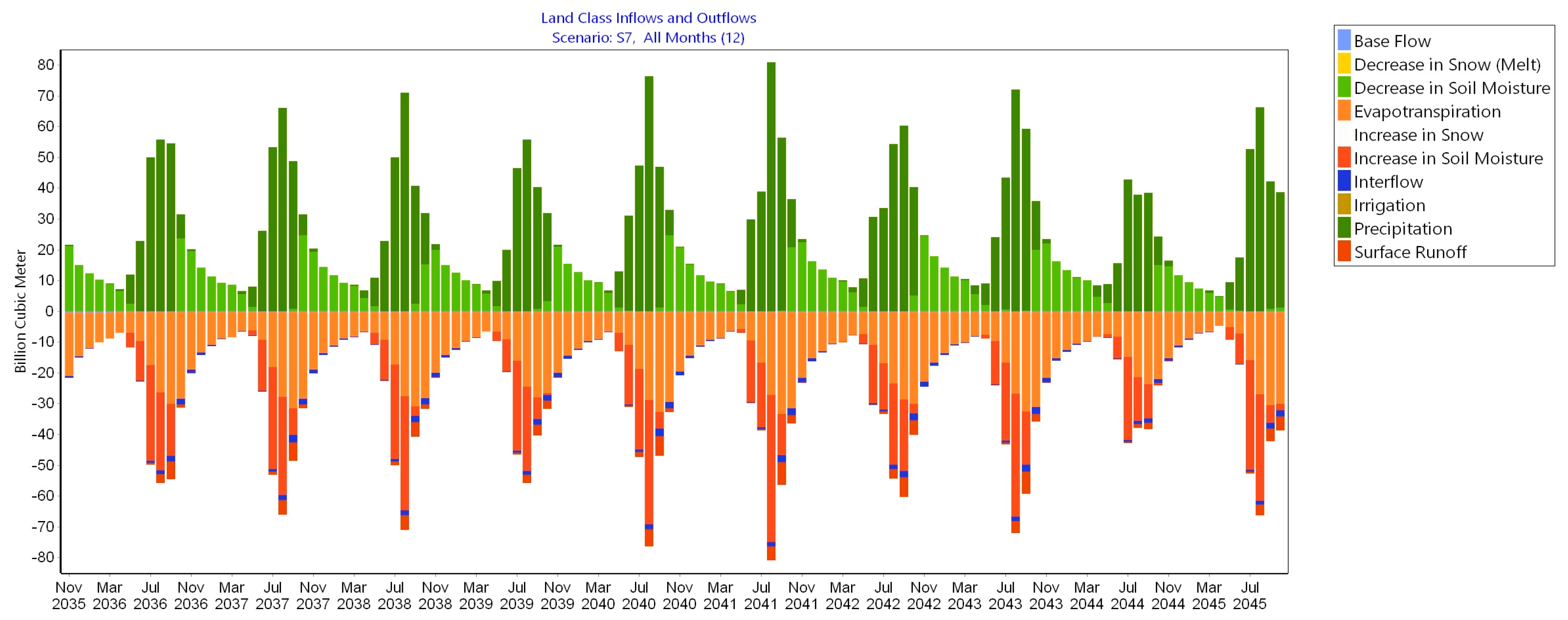
2.3.2. The Temporal Disaggregation

In order to effectively monitor the level of water stress, it is necessary to assess this indicator across a range of time scales, going beyond monthly analyses [11] and focusing on the different seasons where variations in water availability and utilisation become significant. Consequently, it is imperative to calculate SDG 6.4.2 by basin and by season, implementing not only a spatial but also a temporal disaggregation approach.

Under short-term conditions, changes in soil water storage cannot be considered negligible anymore, and the water balance equation for a generic hydrologic unit (i) and time (s) becomes:

$$\mathrm{P}(\mathrm{i},\mathrm{s}) - \mathrm{ET}(\mathrm{i},\mathrm{s}) - \mathrm{R}(\mathrm{i},\mathrm{s}) - \mathrm{G}(\mathrm{i},\mathrm{s}) = \Delta \mathrm{G}(\mathrm{i},\mathrm{s}) \left[{\mathrm{m}}^3\right]$$

(18)

where P(i,s) is the precipitation, ET(i,s) is the actual evapotranspiration including natural vegetation, agriculture under rainfed conditions, evaporation from bare soil and from open water, wetlands and swamps, R(i,s) is the runoff or drainage, G(i,s) is the groundwater recharge and ∆S(i,s) is the change in soil water storage, which reflects the increase ($-$) and decrease (+) of the soil moisture during the time period considered (s).

To implement a seasonal estimation of the level of water stress, it becomes necessary to also consider the water released and stored in the reservoirs, which plays a key role in the accounting for the water resources available per season in each SB. Therefore, IRWR is defined as follows:

$$\begin{array}{c}\mathrm{I}\mathrm{R}\mathrm{W}\mathrm{R} \left(\mathrm{i},\mathrm{s}\right) = \mathrm{R}\left(\mathrm{i},\mathrm{s}\right) + \mathrm{G}\left(\mathrm{i},\mathrm{s}\right) + ∆\mathrm{S}\left(\mathrm{i},\mathrm{s}\right) + \mathrm{d}\mathrm{e}\mathrm{c}\mathrm{r}\mathrm{e}\mathrm{a}\mathrm{s}\mathrm{e} \mathrm{i}\mathrm{n} \mathrm{r}\mathrm{e}\mathrm{s}\mathrm{e}\mathrm{r}\mathrm{v}\mathrm{o}\mathrm{i}\mathrm{r} \mathrm{s}\mathrm{t}\mathrm{o}\mathrm{r}\mathrm{a}\mathrm{g}\mathrm{e}(\mathrm{i},\mathrm{s}) - \\ \mathrm{i}\mathrm{n}\mathrm{c}\mathrm{r}\mathrm{e}\mathrm{a}\mathrm{s}\mathrm{e} \mathrm{i}\mathrm{n} \mathrm{r}\mathrm{e}\mathrm{s}\mathrm{e}\mathrm{r}\mathrm{v}\mathrm{o}\mathrm{i}\mathrm{r} \mathrm{s}\mathrm{t}\mathrm{o}\mathrm{r}\mathrm{a}\mathrm{g}\mathrm{e}(\mathrm{i},\mathrm{s}) \left[{\mathrm{m}}^3\right]\end{array}$$

(19)

where a decrease and increase in reservoir storage implies more (positive) or less water (negative) internally available for SB(i) during season s.

Equation (17a) for an SB(i) and for a season (s), becomes:

$$\begin{array}{c}\mathrm{T}\mathrm{R}\mathrm{W}\mathrm{R} \left(\mathrm{i},\mathrm{s}\right) = \mathrm{R}\left(\mathrm{i},\mathrm{s}\right) + \mathrm{G}\left(\mathrm{i},\mathrm{s}\right) + ∆\mathrm{S}(\mathrm{i},\mathrm{s}) + \mathrm{d}\mathrm{e}\mathrm{c}\mathrm{r}\mathrm{e}\mathrm{a}\mathrm{s}\mathrm{e} \mathrm{i}\mathrm{n} \mathrm{r}\mathrm{e}\mathrm{s}\mathrm{e}\mathrm{r}\mathrm{v}\mathrm{o}\mathrm{i}\mathrm{r} \mathrm{s}\mathrm{t}\mathrm{o}\mathrm{r}\mathrm{a}\mathrm{g}\mathrm{e} \left(\mathrm{i},\mathrm{s}\right) - \mathrm{i}\mathrm{n}\mathrm{c}\mathrm{r}\mathrm{e}\mathrm{a}\mathrm{s}\mathrm{e} \mathrm{i}\mathrm{n} \mathrm{r}\mathrm{e}\mathrm{s}\mathrm{e}\mathrm{r}\mathrm{v}\mathrm{o}\mathrm{i}\mathrm{r} \mathrm{s}\mathrm{t}\mathrm{o}\mathrm{r}\mathrm{a}\mathrm{g}\mathrm{e}(\mathrm{i},\mathrm{s}) + \\ \mathrm{U}\mathrm{p}\mathrm{s}\mathrm{t}\mathrm{r}\mathrm{e}\mathrm{a}\mathrm{m} \mathrm{R}\mathrm{e}\mathrm{q}\left(\mathrm{i},\mathrm{s}\right) - \mathrm{D}\mathrm{o}\mathrm{w}\mathrm{n}\mathrm{s}\mathrm{t}\mathrm{r}\mathrm{e}\mathrm{a}\mathrm{m} \mathrm{r}\mathrm{e}\mathrm{s} \left(\mathrm{i},\mathrm{s}\right) + \mathrm{I}\mathrm{m}\mathrm{p}\mathrm{o}\mathrm{r}\mathrm{t}\mathrm{e}\mathrm{d} \mathrm{w}\mathrm{a}\mathrm{t}\mathrm{e}\mathrm{r}\left(\mathrm{i},\mathrm{s}\right) - \mathrm{E}\mathrm{x}\mathrm{p}\mathrm{o}\mathrm{r}\mathrm{t}\mathrm{e}\mathrm{d} \mathrm{w}\mathrm{a}\mathrm{t}\mathrm{e}\mathrm{r} \left(\mathrm{i},\mathrm{s}\right) [{\mathrm{m}}^3/\mathrm{year}]\end{array}$$

(20)

2.4. Total Freshwater Withdrawals

The total freshwater withdrawals can be defined as:

$$\mathrm{T}\mathrm{F}\mathrm{W}\mathrm{W}\left(\mathrm{i},\mathrm{s}\right) = \mathrm{S} \mathrm{w}\mathrm{i}\mathrm{t}\mathrm{h}\mathrm{d}\mathrm{r}\mathrm{a}\mathrm{w}\mathrm{a}\mathrm{l}\mathrm{s} \left(\mathrm{i},\mathrm{s}\right) + \mathrm{G} \mathrm{w}\mathrm{i}\mathrm{t}\mathrm{h}\mathrm{d}\mathrm{r}\mathrm{a}\mathrm{w}\mathrm{a}\mathrm{l}\mathrm{s} \left(\mathrm{i},\mathrm{s}\right) [{\mathrm{m}}^3/\mathrm{year}]$$

(21)

where S withdrawals (i) and G withdrawals(i) are, respectively, the surface and groundwater withdrawals of the hydrologic unit (i) during the season s.

According to the SDG indicator 6.4.2 metadata, TFWW are all the withdrawals from freshwater and fossil groundwater, but it does not include direct use of non-conventional water, such as direct use of treated wastewater, agricultural drainage water and desalinated water [20]. TFWW refers to the sum of freshwater withdrawals in the main economic sectors, which, as defined by the International Standard Industrial Classification (ISIC), include agriculture; forestry and fishing; manufacturing; electricity industry; and services.

$$\mathrm{TFWW}(\mathrm{i},\mathrm{s}) = {\mathrm{V}}_{\mathrm{A}} (\mathrm{i},\mathrm{s}) + {\mathrm{V}}_{\mathrm{S}} (\mathrm{i},\mathrm{s}) + {\mathrm{V}}_{\mathrm{M}} (\mathrm{i},\mathrm{s}) \left[{\mathrm{m}}^3\right]$$

(22)

where V_A, V_S and V_M are the volumes of freshwater withdrawals, respectively, in the agriculture, service and the industrial sectors (m³). V_S is usually computed as the total freshwater withdrawn by the public distribution networks. V_M is the volume of water withdrawn for mining and quarrying, manufacturing, construction and energy. This sector refers to self-supplied industries not connected to the public distribution network. It includes water for the cooling of thermoelectric and nuclear power plants, but it does not include hydropower [12].

The estimate of the water withdrawal data by SB can be performed using a water supply side or a water demand side approach depending on how the data are collected and aggregated.

A supply-side approach can be applied when the geographical location of the water withdrawal points of each economic sector is well known inside the hydrologic unit. As shown in Figure 6, if we know where, when and how much water is withdrawn, it will be possible to easily disaggregate the water withdrawal of each sector by SB and by season.

A demand-side approach can be applied when data are available aggregated by the administrative level (e.g., region, province or district) for each type of use (agriculture, industry and services); therefore, in order to estimate the water withdrawals, it will be necessary to assess the water demands by SB and then to estimate the withdrawals.

To assess the water use of each hydrological unit, a hydrologic factor per administrative unit has been defined on the basis of the land use/land cover (LULC) map. The hydrologic factor represents the part of a given water use that can be applied to a specific hydrological unit.

Figure 7 shows a typical example where water demand data of an economic sector, for example, industry, is available for an administrative unit whose boundaries intersect different hydrological units. Assuming that the red polygon represents the industrial area included in the administrative unit (grey polygon), if 15 percent of such an industrial area falls in SB B and 85 percent in SB A, then 15 percent of the industrial water demand at the administrative unit level will be allocated to SB B and 85 percent to SB A.

A good and detailed LULC map, consequently, is key to disaggregate at the SB level the statistical data available per administrative unit (e.g., industrial water demand). Together with LULC data, for the services and agriculture sectors, there are other geospatial and remote sensing products that can help in the spatial disaggregation of the data.

For the service sector, where water demands largely depend on the number of people living in a certain area, remote sensing gridded population allows redistributing national or regional census population data in pixels (grid cells). The combination of local census data (e.g., number of people, water use per capita, etc.) with these EO-based products (the global rural-urban mapping project—GRUMPv1 [21,22], the gridded population of the world—GPWv4.11 [23], LandScan [24], WorldPop [25], and the global human settlement population layer—GHS-POP [26] are examples of global population databases derived from satellite images) can support the spatial disaggregation of the V_S (for a more robust approach, population estimates should also include temporary residents, who are usually not included in the census and therefore they are not reflected in the global layers on population). In those situations where people’s capacity to access the public distribution network is limited, this must be considered in the disaggregation of the V_S, which will be different depending on the zone analysed.

For the agriculture sector, the V_A is defined as the volume of water withdrawn for the agricultural sector, including irrigation (inclusive of nurseries), livestock (watering and cleaning), and freshwater aquaculture [12] (Equation (23)).

V_A = V_A-irr + V_A-livestock + V_{A-aquaculture} [m³/year]

(23)

In many countries, most water withdrawals in agriculture are due to irrigation (V_A-irr), and when measured data are not available, water demands can be used to estimate V_A-irr. Alternatively, to evaluate V_A-irr, satellite data can be used to estimate the extent of irrigated land, available in some LULC maps, and the water consumed in agriculture, whose proxy is the actual Evapotranspiration (ET).

Through the actual evapotranspiration (ET) modelling, it is now possible to estimate the water consumed not only by irrigated agriculture but also by rainfed agriculture, natural vegetation including forests, bare soil, open water and wetlands. The big limitation of this approach is that we are assuming that water is abstracted where it is consumed, which is not always true.

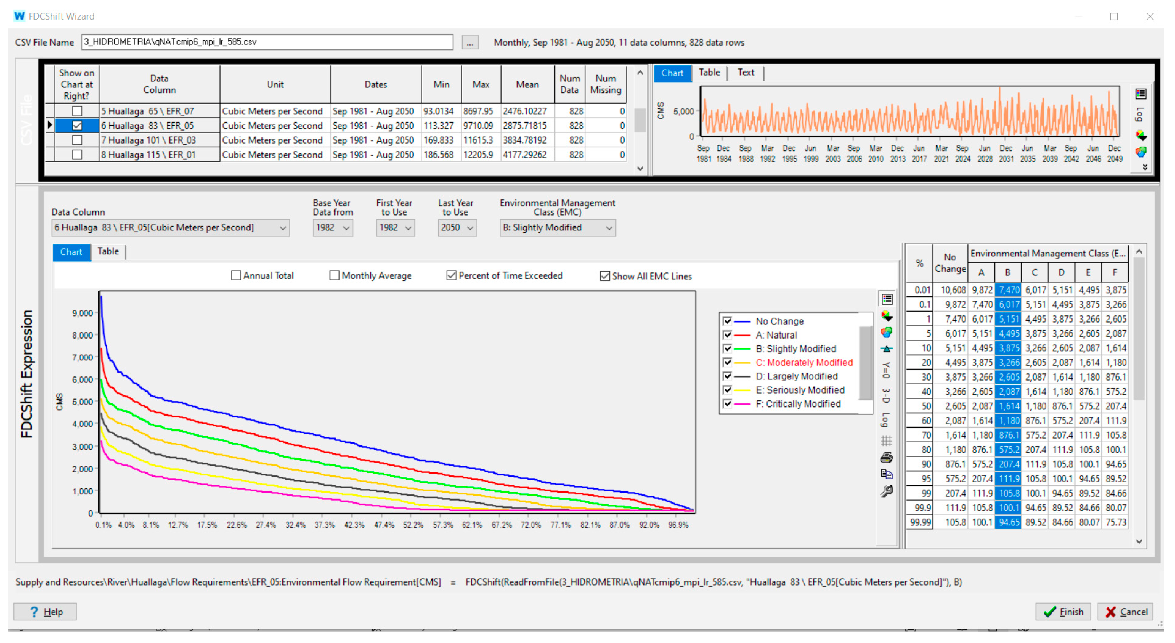
2.5. The Environmental Flow Requirements

For the purpose of calculating the SDG indicator 6.4.2, environmental flows are defined as “…the quantity and timing of freshwater flows and levels necessary to sustain aquatic ecosystems which, in turn, support human cultures, economies, sustainable livelihoods, and wellbeing” (adapted from [27]).

This concept of maintaining the aquatic habitats and ecological processes of a river in a “desirable state”, alternatively referred to as “Environmental Management Classes (EMCs)”, can be defined as the “ecological condition of a river in terms of the deviation of biophysical components from the natural reference condition that will result from implementation of a particular management objective” [28].

Several methods exist for determining environmental flows. The present study calculates the EFR for a hydrological unit applying the flow duration curve shift approach (FDC-Shift) [29,30], which is consistent with the methodological approach used in the Global Environmental Flow Information System (GEFIS) developed by IWMI [31,32] and presented in the FAO Guidelines [28].

Applying the method needs monthly flow data and the construction of a flow duration curve over the simulation period. It is also important that the FDC is consistent with the flows generated within the scenarios under consideration. If the FDC is generated using another data set, then it is likely that the EFRs will not align with the hydrology used in the simulation.

In practice, the FDC-Shift method is implemented through a stepwise adjustment of the FDC, thus reducing the total environmental flows with a decrease in the EMC, while preserving certain characteristics of natural flow variability (Figure 8). On the contrary, high EMCs (e.g., class A) require greater river flow levels to maintain the ecosystem and preserve flow variability (Figure 8). To calculate the SDG 6.4.2, it is necessary to assess the EFR that is required to keep the ecosystem in its present condition (present-day EMC).

The FDC-Shift method comprises four subsequent steps as follows: (i) simulation of reference hydrological conditions in a pristine condition, (ii) definition of environmental management classes (EMCs), (iii) establishment of environmental FDCs from reference conditions and (iv) simulation of continuous monthly time series of environmental flows [33].

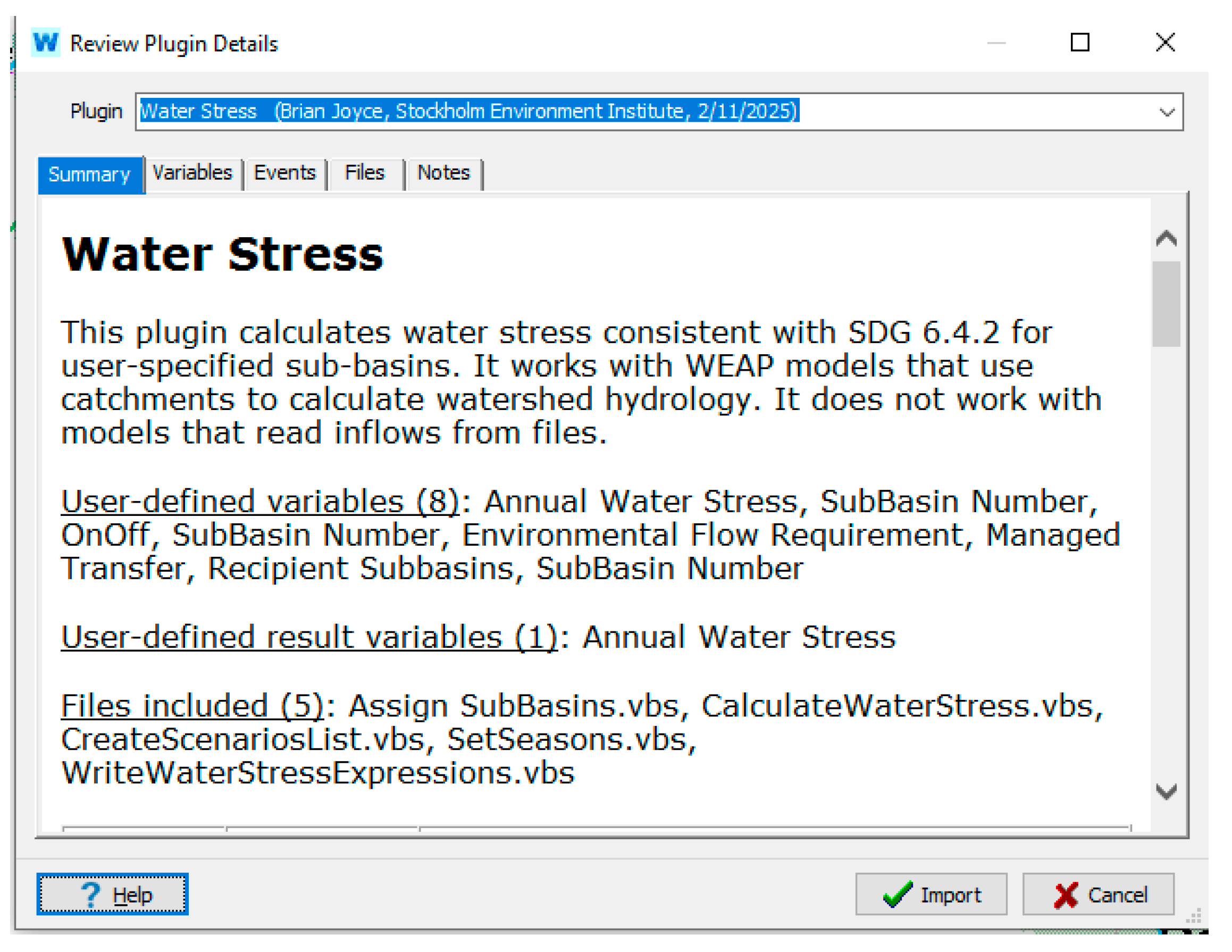
3. The WEAP Water Stress Plugin

To accurately assess water stress by hydrologic unit and season, it is essential to know the specific characteristics of the water system (e.g., the river basin) under analysis. This includes accounting for all factors that influence the estimation of TRWR, TFWW and EFRs. The WEAP (Water Evaluation and Planning System) is suitable to integrate these types of data to produce a practical “water accounting framework” for planners and decision-makers [34]. Accurate assessment requires data collection at a finer temporal scale, such as monthly intervals. While these calculations can be performed using standard spreadsheet tools, more complex systems may benefit from specialised tools such as the water stress plugin (WSP). Developed by FAO in collaboration with the U.S. Centre of the Stockholm Environment Institute (SEI), the WSP operates within WEAP. The initial version of the WSP, which supports the spatial disaggregation of SDG 6.4.2 on an annual basis, has already been published, and it is downloadable online [19] in three languages (English, Spanish and French). An updated version, which includes temporal disaggregation, will be released online soon.

The WEAP is widely used as the planning and management platform in many countries [35,36,37], adopted by public institutions to identify water resources management strategies in response to the impact of climate change, land use change and population growth. It simulates water demand, supply, runoff, infiltration, crop requirements, flows, storage, pollution generation, treatment, discharge and instream water quality [38] under varying hydrologic and policy scenarios [35,36,37].

In WSP, the SDG 6.4.2 is expressed as a percentage between 0 and 100, where a water stress value of 100 percent indicates that all the available freshwater resources, after having taken into account EFR, are being withdrawn, indicating a high level of water stress.

The WSP was designed as a feature that can be imported into any WEAP application (Figure 9). Once it is imported into the WEAP, the WSP calculates SDG 6.4.2 at annual and seasonal timesteps for each SB within a basin for each scenario identified by the user. The WSP results are presented in different formats such as text file, table, chart and map (the WEAP plugin manual is available in English, French and Spanish and can be downloaded on the FAO IMI-SDG6 website https://openknowledge.fao.org/items/68b560ca-d052-42aa-b8f2-514b5b419376, accessed on 5 December 2024).

The WEAP uses a collection of model objects (i.e., catchments, rivers, canals, reservoirs and groundwater) to simulate the movement of water through a basin, with each object contributing in some way to the water balance, both at the basin-wide and at the sub-basin scale. Thus, the stocks and flows of water associated with each WEAP object are needed for the calculation of the variables of the water stress equation.

The EFR is represented as a flow requirement object that behaves as a demand object, which is assigned a demand priority to determine the order in which it is allocated water vis-à-vis other water uses.

The identification of the Flow Requirement objects is a critical step in the proper use of the WSP and has to be performed as the first thing when installing the plugin. Each SB must be assigned an EFR object, which has to be placed at the most downstream point of each sub-basin. This is to ensure that water used to satisfy consumptive demands (TFWW) within an SB is not already used to meet the SB’s EFR, which would conflict with the equation of water stress. Moreover, EFRs should be given the highest priority to ensure that they are fully met when the plugin calculates the volume of water available for withdrawals (TFWW).

EFRs can be defined locally by SB. If that is not possible, the WEAP allows estimating the EFR through the FDC-Shift method, described in the previous section (Figure 10).

Similarly, to estimate the IRWR, we need to know cumulative precipitation and evapotranspiration. The WEAP, through its hydrologic models, simulates all the components of the water balance, including the spatial distribution of soil water storage, surface runoff, and groundwater recharge. In addition, the WEAP considers changes in reservoir storage, which can be positive when resources are released in the system (decrease in reservoir storage) and negative when they are stored in the reservoir (increase in reservoir storage), as shown in Equation (19).

To assess the TRWR, the WSP implements the methodology described in the previous sections, which outlined how the double counting of the freshwater resources is avoided and how water surplus from upstream SBs can be used to cover the water deficit of downstream SBs. In this framework, SBs may forgo using their water surplus and leave water in the river for use downstream (ERWR riverbed). Similarly, water could be transferred to downstream SBs via a canal or pipeline (ERWR canal). In all cases, those transfers appear as part of the TRWR (Equation (20)).

As it was conceived, the methodology developed to avoid double counting implies that the SBs with water deficits receive only the water resources strictly necessary to cover their water demands, including EFR, not a drop more (Equations (15) and (16)). Consequently, these SBs, while covering their needs, will always have 100% water stress, which is correct considering their strong dependency on the water generated in SBs upstream with no deficit. However, water managers may have the necessity of allocating an extra quota of water to SBs with water deficits to respond to specific policy regulations. To this purpose, a new “managed transfer” function was implemented in the last version of the WSP. This function allows the water manager to manually set the water to be transferred into the riverbed from one or more SBs upstream with water surplus to one or more SBs downstream with water deficits.

To calculate the total freshwater withdrawn (TFWW), we need to know direct river abstractions and groundwater pumping for each SB during the analysed season. These data will be represented in the WEAP by demand objects to which a priority will be assigned. When data on withdrawals are not available, water demands become a good proxy for the assessment of indicator 6.4.2.

This plugin complements and integrates information provided by the previous assessment of the indicator at major river basins. It enhances the previous analysis with additional spatial and temporal detail that supports better-informed decisions for a variety of operational scales. The plugin was tested in Tunisia, Algeria, Rwanda, Peru and in the countries sharing the Senegal River basin (Mali, Guinea, Senegal and Mauritania). The application of the WSP for the Senegal River basin is presented below.

3.1. SDG 6.4.2—Level of Water Stress in the Senegal River Basin

3.1.1. Presentation of the Study Area

The Senegal River Basin (SRB) (Figure 11) covers an area of over 424,000 square kilometres, extending across the territories of Guinea, Mali, Mauritania and Senegal. The basin is subdivided into nine sub-catchment areas, encompassing the lower Senegal River valley, the middle Senegal River valley, and the catchment areas of tributaries including Bafing, Baoulé-Bakoye, Falémé, Ferlo, Terekole, Magui Kolimbiné, Karakoro and Gorgol.

Rainfall in the SRB is characterised by significant spatial variability, with a pronounced decrease in precipitation from south to north. Consequently, the majority of the runoff from the Senegal River is contributed by the upper basin, while water inputs are comparatively negligible in the middle and lower valleys. The elevated water levels observed in the valley are attributable to the propagation of flows from the upper basin. The average flow of the Senegal River at its outlet is estimated at 11,900 km³/year. In order to manage the large quantities of water available as effectively as possible, a number of control structures have been installed in the SRB. The most significant of these are the Manantali dam, which was commissioned in 1988 for irrigation and equipped with a 200 MW hydroelectric power station in 2001, and the Diama dam, which was commissioned in 1986. In comparison with natural flows, the flows influenced by the Manantali dam are elevated during periods of low water, at the onset of flooding and at the cessation of flooding (from approximately mid-November to mid-July) and diminished during flooding (from around mid-July to mid-November). Conversely, the Diama dam has been engaged in the regulation of saline intrusion since 1986 by maintaining a permanent freshwater reserve upstream of the dam and lowering the flood level at Diama.

The ecosystems of the SRB can be grouped into four relatively homogeneous clusters, which are delineated as follows: (i) the Fouta Djallon ecosystems in Guinea and southern Mali, which cover 800,000 ha of dense dry forest, including 50,000 ha of forest remnants and numerous valuable wetlands; (ii) the Sudano-Guinean savannah ecosystems along the tributaries of the Senegal River, in Upper Guinea and Mali, consisting of armoured plateaux, alluvial plains and lowlands; and (iii) the freshwater ecosystems found around surface waters in the Senegal River valley, in particular the Walos, flooded areas with high yield potential. (iv) the ecosystems of the delta zone, constituted by salt and brackish water wetlands, which provide a habitat for mangrove formations, a few hectares of mangrove stands and a reception area for migratory birds.

According to the SRB master plan for water development and management up to 2050 (Schema Directeur d’Amenagement et de Gestion des Eaux—SDAGE 2050), the population of the basin is projected to rise from 7.5 to 11.2 million between 2020 and 2050. A considerable proportion of the population is likely to continue to depend on the main rivers for essential services such as drinking water, irrigation, fishing and hydroelectric power. The overall trend for the future is towards increased abstraction, as evidenced by estimates for 2020 which reveal that only around 30% of natural run-off is being used. By the year 2050, demand for drinking water is expected to double, approaching 100% of the current demand, as is the area to be irrigated, which will rise from approximately 200,000 hectares to 410,000 hectares. Furthermore, the potential for hydropower in the basin, which is currently 400 MV (260 MW at Manantali and 140 MW), is anticipated to be doubled or even tripled through the development of additional dams, such as Koukoutamba and Gourbassi, which are scheduled for construction in the near future, along with Balassa and Boureya in the long term.

In the context of the development of transboundary water resources, the “Organisation de Mise en valeur du bassin du fleuve Sénégal” (OMVS) and its member states (Senegal, Mali, Guinea, and Mauritania) will be required to ensure the availability of water in sufficient quantity and quality for human uses and for ecosystems, whilst taking into account the effects of climate change. The development of the WEAP model for the Senegal River Basin has been informed by this overarching objective.

3.1.2. Scenario Development

The WEAP-SRB model incorporates two levels of development extracted from the SDAGE 2050. Firstly, the current situation (SA) is based on maintaining the trends recorded in 2020. Secondly, the optimised situation (S7) presents a balanced compromise in the development of drinking water supply, irrigation, navigation and hydroelectricity.

The overarching objective of the SDAGE 2050 is to ensure that the management of water resources within the basin plays a pivotal role in the region’s developmental initiatives. In the immediate future (2025), this objective entails the assurance of drinking water supply to 7.5 million individuals, the operationalisation of the 200,000 hectares of already-prepared agricultural land, the fulfilment of the water requirements of 31 million TLUs (Tropical Livestock Units, standardised units used to compare different livestock herds by converting various animals to a common metric, with 1 TLU representing a 250 kg animal) and the satisfaction of the demand of the mining industry. Furthermore, the Senegal River should be navigable for part of the year, with flows corresponding to one tenth of the modulus of the Manantali operations and 52 m³/s at Bakel being reserved for the environment, while ensuring the smooth operation of the existing dams, including the Gouina dam. In the long term, by the year 2050, the objective is to supply drinking water to 11.2 million people and water to 115 million TLUs. It is planned that the entire irrigable potential, amounting to 400,000 hectares, will be exploited and that the capacity of active mines will be more than doubled. In order to meet environmental requirements, it will be necessary to ensure that the target low-water flow at Bakel is achieved, in addition to the target flood flow. It is anticipated that hydroelectricity will undergo moderate development with the completion of the Koukoutamba and Gourbassi dams.

Table 4. Water needs for each SDAGE 2050 scenario considered in the WEAP-SRB model. Source: authors’ elaboration.

		SA	S7
Drinking water supply (Mm3)	Directly inside the SRB	116.9	312.3
	Transferred outside the SRB	178	196.2
Livestock (Mm3)		119.7	190.5
Mining (Mm3)		241.1	582.7
Irrigation (Mm3)		3558.4	5918.9
Hydroelectricity	Total storage capacity (Mm3)	11,300	17,000
Environment	Target low-water flow at Bakel (m3/s)	52	52
	Target peak flood flow at Bakel (m3/s)	--	2200
Shipping	Bakel flow between July and January (m3/s)	--	300
	Diama flow between July and January (m3/s)	--	200

provides an overview of water requirements for the two development scenarios.

In the SA and S7 scenarios, environmental management class B is considered for all the sub-basins, with the exception of the Bafing, Moyenne Vallée and Basse Vallée sub-basins, for which class C is taken into account. This is justified by the presence of the Manantali, Gouina and Diama dams, which have altered the river’s natural regime in these sub-basins.

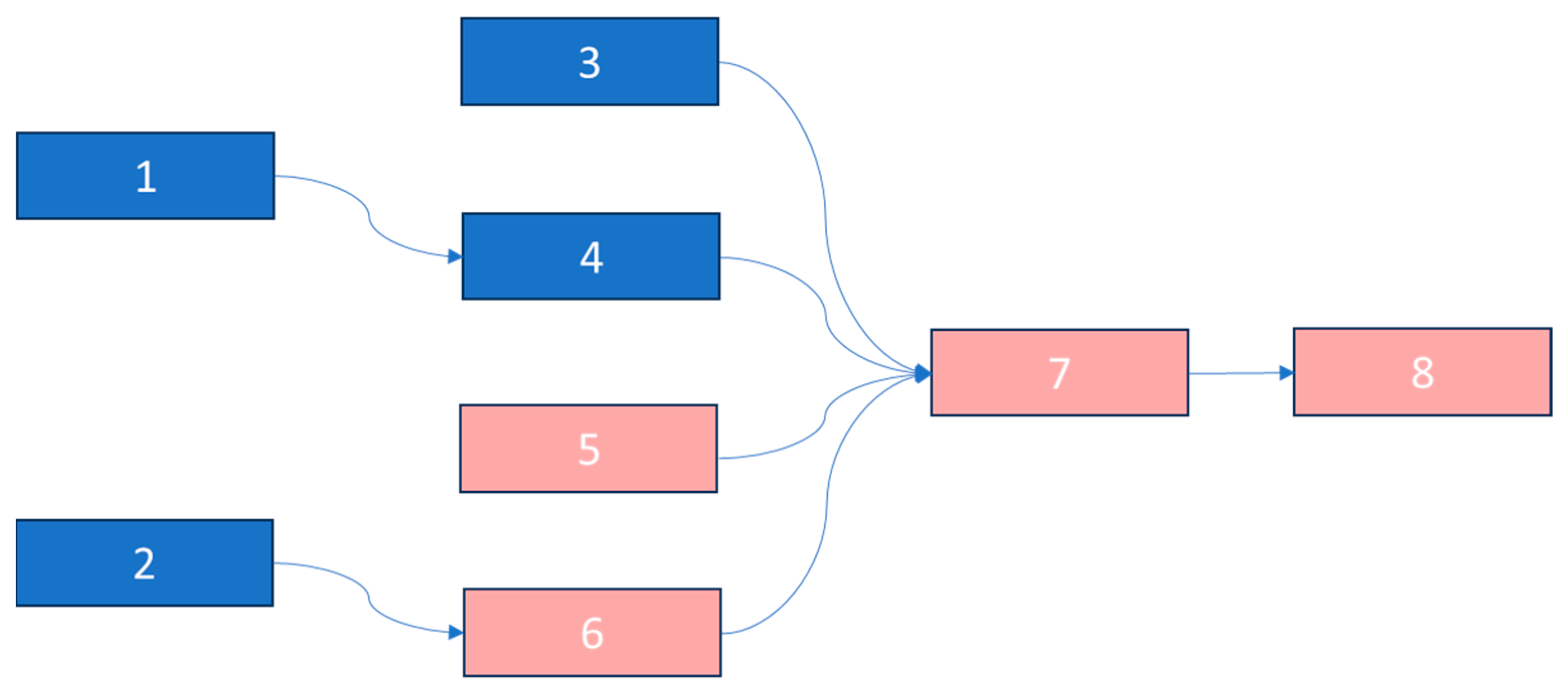
3.1.3. Schematisation of the WEAP Model

The WEAP model used was originally developed by OMVS in 2022-23 to support the plans and strategies included in the Master Plan for Water Development and Management (SDAGE 2050) in the Senegal River Basin. This model has been recently updated by the SEI in collaboration with FAO and OMVS. Data and results of the model have been validated by OMVS, which presented them to the Niger, Volta and Gambia River Basin Authorities in February 2025 during a workshop organised by FAO and OMVS. The schematisation of the updated SRB WEAP model has integrated three sets of elements to ensure a representation that is both accurate and comprehensive. Firstly, the geographical extent was considered, using shapefiles to faithfully reproduce the boundaries of the basin and sub-basins. Next, the physical characteristics of each sub-basin were considered, enabling an analysis of hydrological and environmental conditions and a characterisation of supplies. Finally, all activities present in the sub-basins were considered in relation to water requirements. For each activity, water demand was spatially disaggregated into demand sites according to their position in the sub-basins. Each demand site was linked to a portion of the river via a transmission link and a return flow. However, the city of Dakar constitutes an exception, as it has no return flow, given that it is not located in the SRB. The SRB WEAP is mainly supplied with water by surface runoff, which was determined by hydrological modelling using the WEAP’s soil-moisture method. This modelling was based on open-source climate data, verified with field climate measurements, and the model was calibrated using historical flow data for each sub-basin of the Senegal River and its tributaries. Information pertaining to the regulation infrastructures, in particular the Manantali, Diama and Gouina dams, was integrated in accordance with the historical operating data and the planning according to the SDAGE 2025. The control of environmental flow requirements in the SRB WEAP was implemented at the hydrometric stations.

In accordance with the vision outlined by the SDAGE 2050, a monthly time step was established for the WEAP SRB model. Two seasons were considered, with the dry season lasting eight months, from November to June. The modelling was initiated for the period spanning from 2034 to 2045. However, the initial two years (2034 and 2035) were designated as a warm-up period for the model, and consequently, the results are presented for the period from 2036 to 2045.

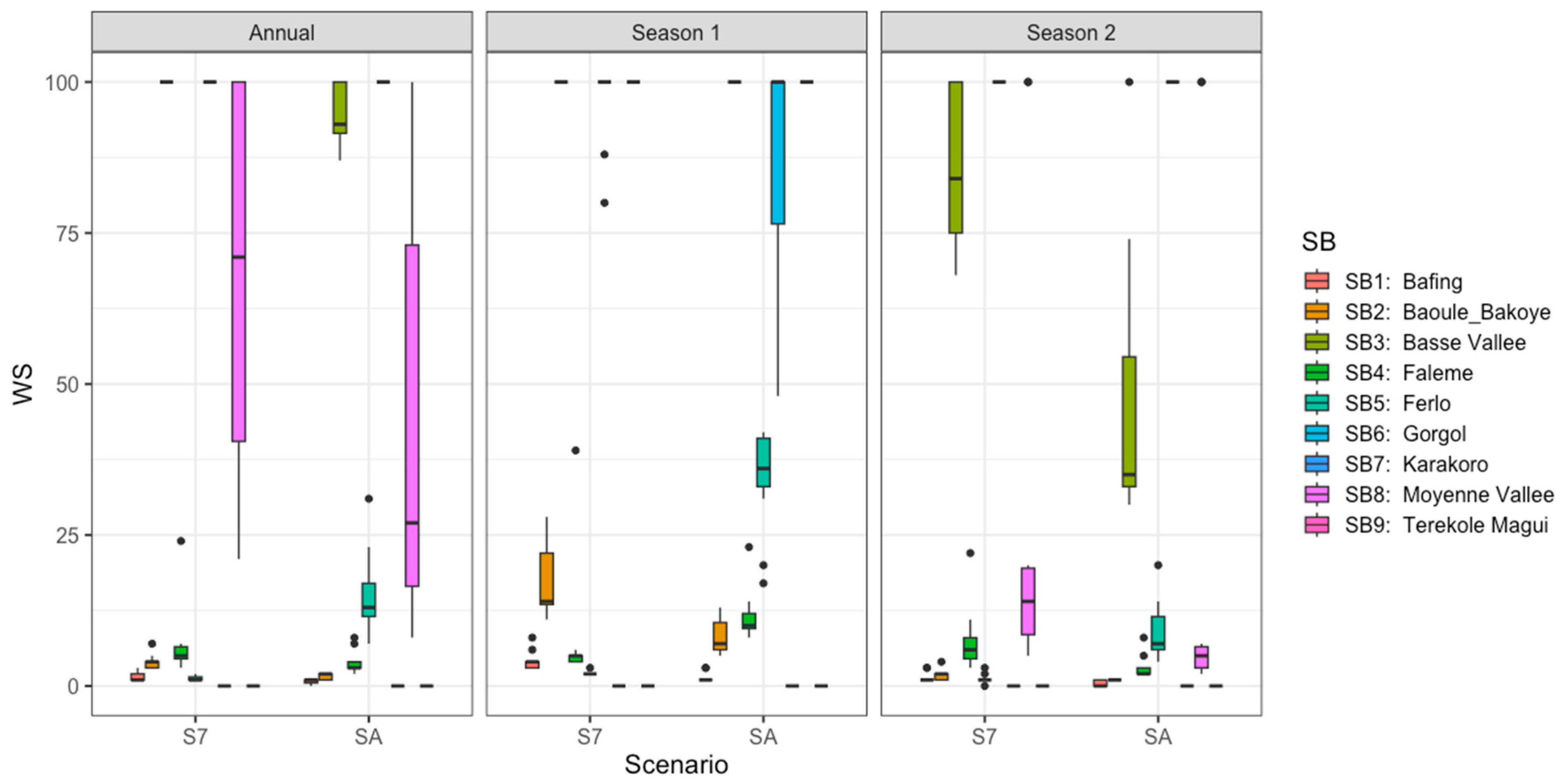
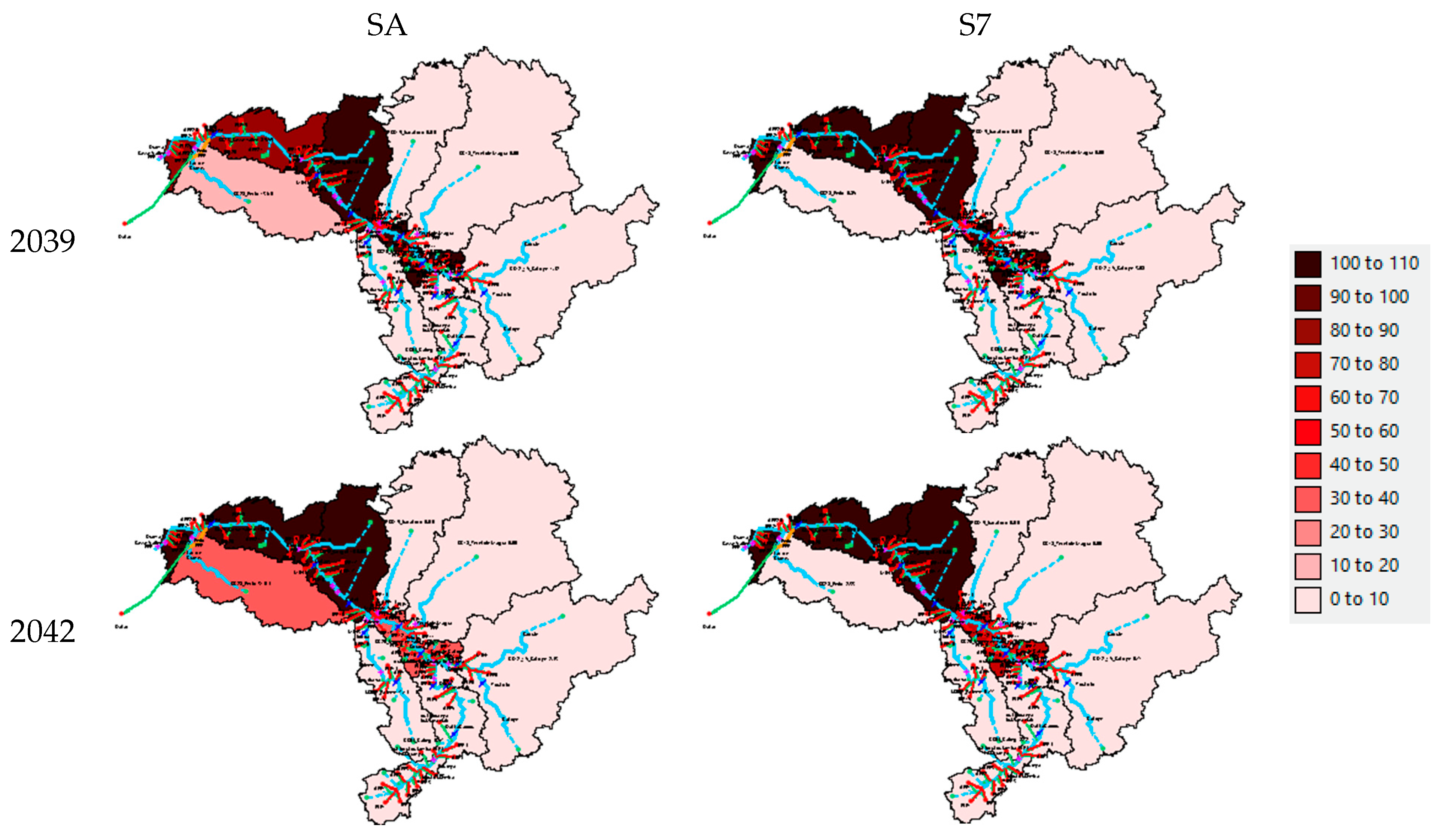
3.1.4. Analysis of the Results of Modelling

The analysis of the water balance for the period 2036–2045, conducted at the catchment scale, demonstrates that the rainfall period extends from July to October (see Figure 12), as considered for the parameterisation of the calculation of indicator SDG 6.4.2. Furthermore, the model shows that, during years of high precipitation, such as 2038 and 2039, rainwater volumes can reach 75 to 80 billion cubic metres (BCM), while in years of low precipitation, such as 2042, these volumes can reach 40 to 45 BCM. It is important to note that almost 50% of these rainfall volumes are generated in the Bafing sub-basin. These findings imply that the Bafing sub-basin will continue to play a pivotal role in the future for the water supply of the Senegal River catchment.

The EFR, determined over the period 2036–2045 (see Figure 13), demonstrates a consistent trend with the flows generated by precipitation, indicating that years with particularly intense rainfall require higher environmental flows. It is noteworthy that EFR for the headwater basins, i.e., the tributaries of the Senegal River, are significantly lower than those required downstream along the Senegal River itself. For example, simulations conducted revealed that, for the years 2038–2039, Basse Vallée, Gorgol and Moyenne Vallée experienced peak EFR of between 1000 and 1800 cubic metres per second (CMS), while the EFR for the Bafing peaked at between 400 and 350 CMS.

The determination of water stress in the SRB revealed that, under both SA and S7 scenarios, the lower basins exhibited elevated levels of water stress. Conversely, the upper basins indicated low to medium levels of stress. A more detailed investigation of water stress in the lower basin discloses that, on an annual basis, water stress in the Basse Vallee and Gorgol is evaluated as extremely high (above 75%), irrespective of the scenario under consideration (see Figure 14). In contrast, the Moyenne Vallee exhibits considerable variability, with values ranging from 8 to 100 in the trend scenario (SA) and from 21 to 100 in the optimised scenario (S7). Figure 15 presents a spatial representation of annual water stress for a year with high rainfall (2039) and a year with low rainfall (2042).

It is worth noting that the SRB as a whole results in a no-water-stress condition (see Figure 1b). The same appears if we consider the national water stress values of the four riparian countries: Guinea, Mali, Mauritania and Senegal (see Figure 1a). It is therefore evident of the additional level of insights gained from the spatial and temporal disaggregation of the indicator.

4. Conclusions

The methodology proposed in this paper allows keeping consistency between the total renewable water resources calculated at basin level and the same calculated as a sum at sub-basin level. With this method, water managers will be able to assess the SDG 6.4.2 by sub-basin and by season, avoiding the double counting of the total renewable freshwater resources. Water supplies of each SB are calculated taking into account either the water demands of downstream SBs or the water requests to upstream SBs in each considered season and hydrologic or policy scenario. This implies that the water accounted for in each hydrologic unit may be different from the water actually flowing.

As it was conceived, the methodology developed to avoid double counting implies that some SBs may experience water deficits while appearing to have plentiful available water supplies because the calculation of deficits accounts for only the water resources generated within the SBs. In fact, these SBs are dependent on water flowing in from upstream SBs, which makes them vulnerable to any changes in water management upstream. Consequently, while covering their needs, they will always have 100% water stress, which is to be considered correct considering their strong dependency on the water generated in SBs upstream with surplus.

The WSP accounts for these inflows and applies to the calculation of water stress only those flows that are strictly necessary to cover the water demands of these SBs, including EFR. However, water managers may have the necessity of allocating an extra quota of water to SBs with water deficits to respond to specific policy regulations. To this purpose, a “managed transfer” function is implemented in the WSP. This function allows the water manager to manually set the volume of water to be transferred via the riverbed from one or more SBs upstream with water surplus and to be allocated to one or more SBs downstream with water deficit. The effect of this will be to reduce the water stress in the downstream SB to some value less than 100 percent, while simultaneously increasing the water stress in the source SB. Integrating the WSP into the WEAP enables the analysis of the level of water stress and the implementation of water accounting across various climate and management scenarios.

By calculating the indicator at the SB level, it is now possible to quickly identify when and where there is an impact on resource sustainability and the potential for conflict among users, which can become essential information for the definition of water management policies in a country.

The disaggregation of water stress and its components is necessary to implement water accounting and auditing of the freshwater resources, which requires strong communication and data exchange between agencies and water/policy experts. In fact, by analysing the data for disaggregating the level of water stress, the users will obtain a better understanding of the spatial and temporal dynamics of the river flow, allowing for better planning of water use over the year. In our opinion, avoiding double counting will allow reducing the risk of overestimating the availability of water resources, and this will give water managers a correct view of the resources they can count on to perform their duties, while policy makers will have a better idea of the variability of the resources, usually hidden behind the long-term averages.

On the practical side, while the plugin is ready to work with the WEAP, the equations presented in this paper can be applied in other systems, including common calculation spreadsheets. However, the methodology is not meant to be self-applicable, and it requires an existing expertise in water accounting and modelling.

In summary, the assessment of the SDG 6.4.2 by SB and by season helps in developing national integrated water management policies, including investment in infrastructure and promoting public awareness. These combined efforts are crucial to ensure the sustainable management of water resources by addressing the challenges of the level of water stress.

References

1. Jury, W.A.; Vaux, H.J., Jr. The emerging global water crisis: Managing scarcity and conflict between water users. Adv. Agron. 2007, 95, 1–76. [Google Scholar]
2. Mishra, R.K. Fresh water availability and its global challenge. Br. J. Multidiscip. Adv. Stud. 2023, 4, 1–78. [Google Scholar] [CrossRef]
3. FAO. The Future of Food and Agriculture—Trends and Challenges; Food and Agriculture Organization of the United Nations: Rome, Italy, 2017; Available online: http://www.fao.org/3/a-i6583e.pdf (accessed on 5 December 2024).
4. FAO. Coping with Water Scarcity. An Action Framework for Agriculture and Food Security. 2012. Available online: http://www.fao.org/3/a-i3015e.pdf (accessed on 5 December 2024).
5. Ahopelto, L.; Veijalainen, N.; Guillaume, J.H.A.; Marko Keskinen, M.; Marttunen, M.; Varis, O. Can There be Water Scarcity with Abundance of Water? Analyzing Water Stress during a Severe Drought in Finland. Sustainability 2019, 11, 1548. [Google Scholar] [CrossRef]
6. United Nations General Assembly. Transforming Our World: The 2030 Agenda for Sustainable Development. 2015. Available online: https://sdgs.un.org/2030agenda (accessed on 5 December 2024).
7. FAO. Integrated Monitoring Initiative for SDG 6 Step-by-Step Monitoring Methodology for Indicator 6.4.2. Version: 4. 2019. Available online: https://openknowledge.fao.org/server/api/core/bitstreams/43ceaf5d-0837-40e6-82d4-98935a75752a/content (accessed on 5 December 2024).
8. Biancalani, R.; Marinelli, M. Assessing SDG indicator 6.4.2 ‘level of water stress’ at major basins level. UCL Open Environ. 2021, 3. [Google Scholar] [CrossRef] [PubMed]
9. FAO and UN-Water. Progress on the Level of Water Stress—Mid-Term Status of SDG Indicator 6.4.2 and Acceleration Needs, with Special Focus on Food Security; Food and Agriculture Organization of the United Nations: Rome, Italy, 2024. [Google Scholar] [CrossRef]
10. Vanham, D.; Hoekstra, A.Y.; Wada, Y.; Bouraoui, F.; de Roo, A.; Mekonnen, M.M.; van de Bund, W.J.; Batelaan, O.; Pavelic, P.; Bastiaanssen, W.G.M.; et al. Physical water scarcity metrics for monitoring progress towards SDG target 6.4: An evaluation of indicator 6.4.2 “Level of water stress”. Sci. Total Environ. 2018, 613–614, 218–232. [Google Scholar] [CrossRef] [PubMed]
11. Hoekstra, A.Y.; Mekonnen, M.M.; Chapagain, A.K.; Mathews, R.E.; Richter, B.D. Global Monthly Water Scarcity: Blue Water Footprints versus Blue WaterAvailability. PLoS ONE 2012, 7, e32688. [Google Scholar] [CrossRef] [PubMed]
12. FAO. AQUASTAT: FAO’s Global Information System on Water and Agriculture. 2021. Available online: http://www.fao.org/aquastat/en/ (accessed on 23 February 2021).
13. FAO. Hydrological Basins Derived from Hydroshed. 2011. Available online: https://data.apps.fao.org/map/catalog/srv/eng/catalog.search#/metadata/7707086d-af3c-41cc-8aa5-323d8609b2d1 (accessed on 1 March 2020).
14. Karimi, P.; Bastiaanssen, W.G.M.; Molden, D. Water Accounting Plus (WA+)—A water accounting procedure for complex river basins based on satellite measurements. Hydrol. Earth Syst. Sci. Discuss. 2013, 9, 12879–12919. [Google Scholar] [CrossRef]
15. Batchelor, C.; Hoogeveen, J.; Faurès, J.M.; Peiser, L. Water Accounting and Auditing: A Sourcebook; FAO Water Reports No. 43; Food and Agriculture Organization of the United Nations: Rome, Italy, 2016. [Google Scholar]
16. OECD. Water Resources Allocation: Sharing Risks and Opportunities; OECD Studies on Water; OECD Publishing: Paris, UK, 2015. [Google Scholar] [CrossRef]
17. Zhu, Z.; Giordano, M.; Cai, X.; Molden, D. The Yellow River Basin: Water Accounting, Water Accounts, and Current Issues. Water Int. 2004, 29, 2–10. [Google Scholar] [CrossRef]
18. Viessman, W.; Lewis, G.L. Introduction to Hydrology; HarperCollins College Publishers: HarperCollins, NY, USA, 1996. [Google Scholar]
19. FAO. Water Stress Plugin for Water Evaluation and Planning System (WEAP). Using the Water Evaluation and Planning Tool for the Calculation of Sustainable Development Goal Indicator 6.4.2; Food and Agriculture Organization of the United Nations: Rome, Italy, 2024. [Google Scholar] [CrossRef]
20. UNSD. Metadata of Indicator 6.4.2. 2024. Available online: https://unstats.un.org/sdgs/metadata/files/metadata-06-04-02.pdf (accessed on 5 December 2024).
21. Balk, D.L.; Deichmann, U.; Yetman, G.; Pozzi, F.; Hay, S.I.; Nelson, A. Determining Global Population Distribution: Methods, Applications and Data. Global Mapping of Infectious Diseases: Methods, Examples and Emerging Applications. Adv. Parasitol. 2006, 62, 119–156. [Google Scholar] [CrossRef] [PubMed]
22. CIESIN. Global Rural-Urban Mapping Project. 2020. Available online: https://sedac.ciesin.columbia.edu/data/collection/grump-v1 (accessed on 1 March 2020).
23. CIESIN. Gridded Population of the World, Version 4 (GPWv4); Population Density Adjusted to Match 2015 Revision of UN WPP Country Totals, Revision 10. NASA Socioeconomic Data and Applications Center (SEDAC): Palisades, NY, USA, 2017. Available online: https://sedac.ciesin.columbia.edu/data/collection/gpw-v4 (accessed on 1 March 2020).
24. Landscan Global. Oak Ridge National Laboratory. 2019. Available online: https://landscan.ornl.gov/ (accessed on 1 March 2020).
25. WorldPop. Open Spatial Demographic Data and Research. 2020. Available online: https://www.worldpop.org/ (accessed on 1 March 2020).
26. GHS Population Grid. European Commission, Joint Research Center. 2020. Available online: https://ghslsys.jrc.ec.europa.eu/ghs_pop.php (accessed on 1 March 2020).
27. Arthington, A.H.; Bhaduri, A.; Bunn, S.E.; Jackson, S.; Tharme, R.E.; Tickner, D.; Young, W.; Acreman, M.; Natalie Baker, N.; Capon, S.; et al. The Brisbane Declaration and Action Agenda on Environmental Flows. Front. Environ. Sci. 2018, 6, 45. [Google Scholar] [CrossRef]
28. FAO. Incorporating Environmental Flows into “Water Stress” Indicator 6.4.2—Guidelines for a Minimum Standard Method for Global Reporting; Food and Agriculture Organization of the United Nations: Rome, Italy, 2019; 32p. [Google Scholar]
29. Smakhtin, V.; Anputhas, M. An Assessment of Environmental Flow Requirements of Indian River Basins; IWMI Research Report 107; International Water Management Institute (IWMI): Colombo, Sri Lanka, 2006; 42p. [Google Scholar]
30. Smakhtin, V.U.; Eriyagama, N. Developing a software package for global desktop assessment of environmental flows. Environ. Model. Softw. 2008, 23, 1396–1406. [Google Scholar] [CrossRef]
31. Sood, A.; Smakhtin, V.; Eriyagama, N.; Villholth, K.G.; Liyanage, N.; Wada, Y.; Ebrahim, G.; Dickens, C. Global Environmental Flow Information for the Sustainable Development Goals; IWMI Research Report 168; International Water Management Institute (IWMI): Colombo, Sri Lanka, 2017; 37p. [Google Scholar] [CrossRef]
32. Eriyagama, N.; Messager, M.L.; Dickens, C.; Tharme, R.; Stassen, R. Towards the Harmonization of Global Environmental Flow Estimates: Comparing the Global Environmental Flow Information System (GEFIS) with Country Data; IWMI Research Report 186; International Water Management Institute (IWMI): Colombo, Sri Lanka, 2024; 53p. [Google Scholar] [CrossRef]
33. Shaeri Karimi, S.; Yasi, M.; Eslamian, S. Use of hydrological methods for assessment of environmental flow in a river reach. Int. J. Environ. Sci. Technol. 2012, 9, 549–558. [Google Scholar] [CrossRef]
34. Perry, C.J.; Bucknall, J. Water resource assessment in the Arab world: New analytical tools for new challenges. In Water in the Arab World: Management Perspective and Innovations; Jagannathan, N.J., Mohamed, A.S., Kremer, A., Eds.; The World Bank: Washington, DC, USA, 2009. [Google Scholar]
35. Al-Mukhtar, M.; Mutar, G. Modelling of Future Water Use Scenarios Using WEAP Model: A Case Study in Baghdad City, Iraq. Eng. Technol. J. 2021, 39, 488–503. [Google Scholar] [CrossRef]
36. RaziSadath, P.V.; RinishaKartheeshwari, M.; Elango, L. WEAP Model Based Evaluation of Future Scenarios and Strategies for Sustainable Water Management in the Chennai Basin, India. AQUA-Water Infrastruct. Ecosyst. Soc. 2023, 72, 2062–2080. [Google Scholar] [CrossRef]
37. Yang, L.; Bai, X.; Khanna, N.; Yi, S.; Hu, Y.; Deng, J.; Gao, H.; Tuo, L.; Xiang, S.; Zhou, N. Water evaluation and planning (WEAP) model application for exploring the water deficit at catchment level in Beijing. Desalin. Water Treat. 2018, 118, 12–25. [Google Scholar] [CrossRef]
38. Stockholm Environment Institute (SEI) Website. Available online: https://www.sei.org/tools/weap/ (accessed on 5 December 2024).
Figure 1. Level of water stress (SDG 6.4.2) by country (a) and by major river basin (b). Source: [8].
Water 17 01543 g001
Figure 2. Example of a river basin including 3 SBs: SB A (the head of the basin), SB B and C (downstream). Source: authors’ own elaboration.
Water 17 01543 g002
Figure 3. Example of a river basin including 3 SBs: SB A (head of the basin), SB B and C (downstream), showing the water exchanged between SBs (ERWR), considering the hypothetical water consumed in each SB. Source: authors’ own elaboration.
Water 17 01543 g003
Figure 4. Example of a river basin including 3 SBs: SB A (head of the basin), SB B and C (downstream), showing the water exchanged between SBs (ERWR), considering the hypothetical water withdrawal and consumption of each SB. Source: authors’ own elaboration.
Water 17 01543 g004
Figure 5. Schematic view of a river basin with 8 sub-basins. SB 1 and 2 (head of the basin), SB 7 and 8 (downstream sub-basins). In red are the sub-basins where there is a water deficit, and in blue are those where there is a hypothetical water surplus.
Water 17 01543 g005
Figure 6. Example of a basin including three sub-basins (A, B, C) showing the water supply side approach. Withdrawal points by sector are represented by different symbols. Source: authors’ own elaboration.
Water 17 01543 g006
Figure 7. Example of a basin including three sub-basins (A, B, C) showing the hydrologic factor, used to disaggregate a water demand available at the administrative level, in a water demand by hydrologic unit. The red polygon represents the polygon of an industrial area in a land use/land cover map. Source: authors’ own elaboration.
Water 17 01543 g007
Figure 8. Flow duration curve. Classes A and B represent the unmodified and largely natural conditions, where no or limited modification has occurred or should be allowed. Class C is defined as moderately modified, with limited impact on ecosystem integrity. Largely modified ecosystems (Class D) show considerable, albeit still acceptable, modification from the natural state [29].
Water 17 01543 g008
Figure 9. The water stress plugin of the WEAP (FAO, 2024). Source: authors’ screenshot from the WEAP.
Water 17 01543 g009
Figure 10. FDCShift wizard tool in the WEAP. Source: authors’ screenshot from the WEAP.
Water 17 01543 g010
Figure 11. Representation of the Senegal River Basin (SRB) in the WEAP. Source: authors’ elaboration.
Water 17 01543 g011
Figure 12. Water balance of the Senegal River basin simulated with the WEAP SRB model for the period 2035–2045. Source: authors’ elaboration.
Water 17 01543 g012
Figure 13. Environmental flow requirements for the Senegal River sub-basins simulated with the WEAP SRB model for the period 2026–2045. Source: authors’ elaboration.
Water 17 01543 g013
Figure 14. Boxplot of aggregate values of water stress in the Senegal River basin by sub-basin and season for two development scenarios (trend situation SA and optimised situation S7). Source: authors’ elaboration.
Water 17 01543 g014
Figure 15. Water stress in the Senegal basin in a high rainfall year (2039) and a low rainfall year (2042), created by the WEAP SRB model.
Water 17 01543 g015