LSTM-Based Runoff Forecasting Using Multiple Variables: A Case Study of the Nyang River, a Typical Basin on the Tibetan Plateau

Abstract

Accurate runoff forecasting is crucial for disaster prevention and mitigation, as well as water resource allocation planning. However, the accuracy of runoff forecasting in high mountain watersheds is limited by the complexity of terrain and the scarcity of observation data. In recent years, machine learning models have been widely used for runoff prediction. In order to explore the application effect of the Long Short-Term Memory (LSTM) network in high mountain watersheds, this paper takes the Nyang River Basin (NRB) in a typical watershed on the Qinghai–Tibet Plateau (QTP) as the research object, and uses LSTM models to study the impact of different input variable combinations on runoff prediction under multiple prediction periods. The results indicate that with the extension of the forecast period, the impact of historical runoff on runoff prediction accuracy gradually decreases, while the impact of precipitation and temperature on runoff prediction accuracy gradually increases. When the forecast period exceeds 13 days, the contribution of precipitation increases more significantly. The use of historical runoff and forecasting that includes historical runoff and precipitation yields the most robust results, with good forecasting performance within 25 days of the forecast period. Moreover, the larger the watershed area, the better the runoff forecasting effect.

1. Introduction

Water resources are one of the most precious natural resources on Earth, playing an irreplaceable role in maintaining ecological balance, supporting human survival, and economic development [1,2]. However, with the intensification of global climate change and human activities, various extreme hydrological disasters are becoming increasingly severe [3], causing huge impacts on the ecological environment and socio-economic development. Faced with such a severe hydrological disaster situation, the role of runoff forecasting has become increasingly crucial and indispensable. Accurate runoff forecasting can not only prevent and reduce disasters but can also assist with planning water resource allocation reasonably, achieving sustainable development [4,5].

Currently, runoff forecasting models can generally be divided into hydrological models and machine learning models. Hydrological models simulate the hydrological cycle in nature through mathematical or physical methods. Representative models include the Soil and Water Assessment Tool (SWAT) model from the United States [6], the Tank model from Japan [7], the Hydrologiska Byråns Vattenbalansavdelning (HBV) model from Sweden [8], and the Xin’anjiang model from China [9]. These models not only have detailed physical explanations but also have strong stability. For example, scholars such as Aiswarya Rani Mahanta [10] have used SWAT models and GIS technology to conduct hydrological simulations of the Palar River Basin in India, demonstrating good effectiveness and accuracy in runoff prediction. However, despite the significant achievements of hydrological models in runoff forecasting, they also have problems such as high requirements for initial data quality, high consumption of computational resources, and low efficiency, making them less suitable for runoff areas with complex runoff mechanisms [11].

With the continuous development of 3S technology and artificial intelligence technology, machine learning models are widely used in runoff forecasting due to their lack of understanding of hydrological processes and strong nonlinear capabilities. Common machine learning models include random forest (RF) models [12], support vector machine (SVM) models [13], and artificial neural network (ANN) models [14]. However, research on exploring the most suitable machine learning models for runoff simulation and prediction has been ongoing [15,16], among which the Long Short-Term Memory (LSTM) network model has gained widespread attention for its unique structure and expertise in processing long time series information [17]. In recent years, scholars have achieved significant results in using LSTM models for runoff prediction in multiple watersheds, verifying their superiority in improving prediction accuracy and adapting to complex environments. Compared with traditional machine learning models, LSTM models have certain advantages due to their high prediction efficiency and the requirement for less input data [18,19].

As the “water tower of Asia”, the Qinghai–Tibet Plateau (QTP) is the source of numerous rivers. It has an altitude of over 4000 meters and diverse terrain. Glaciers, snow, and permafrost are widely distributed. At the same time, the scarcity of hydrological stations on the plateau poses great challenges for estimating runoff [20]. At present, runoff prediction on QTP mainly focuses on identifying variables that have a significant impact on runoff changes and exploring and optimizing runoff prediction models that are most suitable for high-altitude watersheds. The use of temperature and precipitation to predict runoff changes has been proven feasible [21], but for models with strong applicability, although the effectiveness and accuracy of ANN and LSTM models have been confirmed [22], there is significant room for improvement in prediction accuracy. Currently, many mathematicians tend to improve forecast accuracy by combining models or improving data quality. For example, combining the advantages of multiple models to build more powerful forecasting models, or improving data quality through data preprocessing, feature engineering, and other means to optimize the predictive performance of the model [23,24]. However, although these methods have improved the forecast accuracy to some extent, how to further optimize the variable combination of model inputs to improve the forecast effect in a more direct and efficient way is still an important direction of current research.

This article takes the Nyang River Basin (NRB) in the QTP as the research object and selects the LSTM model to study the influence of different input variable combinations and model structures on runoff prediction results under multiple forecasting periods. By comparing and analyzing the predicted results, the specific contribution of each input variable to the forecast accuracy can be accurately quantified. At the same time, self-supervised learning is introduced, drawing on its experience in time series prediction fields such as image recognition [25] and weather forecasting, to analyze the rich historical information in runoff data. This article attempts to offer some methodological references for runoff forecasting in high-altitude watersheds on the QTP. It also hopes to provide certain basic methods and data support for global water resource management and disaster prevention, though there is likely much room for improvement.

2. Materials and Methods

2.1. Overview of the Research Area

The NRB (29°28′–30°30′ N, 92°10′–94°35′ E) is located in the Tibet region of China, originates from Chomuliangla on the west side of Mila Mountain, and is one of the five tributaries of the Yarlung Zangbo River basin (Figure 1). The NRB has a total length of 307.5 km and a drainage area of 17,500 km². It is an important river on QTP. The NRB is not only a river with rich natural landscapes but it also carries rich cultural and historical significance. It is known as the mother river of the Gongbu region of Tibet.

NRB is located on the Qinghai-Tibet Plateau and belongs to the Yarlung Zangbo River basin (the red line in Figure 1 indicates the basin boundary). The NRB has a typical plateau cold climate with low temperatures and large temperature differences between day and night. Meanwhile, influenced by the warm and humid air currents of the Indian Ocean, the NRB exhibits significant seasonal variations. From July to September, there is almost daily precipitation in the NRB, and the cloud cover is also very large, resulting in the peak being shrouded in clouds and mist all day long. The NRB is rich in water, with an annual runoff of 22 billion m³, which makes it one of the important tributaries of the Yarlung Zangbo River. In addition, the forest resources in the NRB are abundant, with high vegetation coverage, which plays an important role in regulating the climate and maintaining the local environment.

2.2. Data Fundamentals

The NRB is a typical area with a lack of data, and precipitation observation data at stations are extremely scarce. There are four observation stations in the basin, and the study collected and used flow and meteorological data from three of them, namely Gongbujiangda, Baheqiao, and Gengzhang (

Table 1. Data from control stations in the Niyang River Basin.

Basin	Control Station	Watershed Area/10,000 km2	Training Set	Validation Set
NRB	Gongbujiangda	6398.70	1 January 2010–31 December 2013	1 January 2014–31 December 2015
	Gengzhang	4998.93
	Baheqiao	4164.18

). Hydrological station data are from the Tibet Hydrological Bureau, and meteorological data are from the website of the National Meteorological Administration, https://data.cma.cn/ (accessed on 13 March 2024).

Considering that the NRB is a high mountain basin and is affected by snowmelt in winter and spring, this study used the training set from 1 January 2010 to 31 December 2013 (Table 1) and the validation set from 1 January 2014 to 31 December 2015. The forecast features include temperature, air pressure, relative humidity, wind speed, sunshine and precipitation, and the target term is daily runoff. The forecast stations are Baheqiao, Gengzhang, and Gongbujiangda.

2.3. Research Methods

2.3.1. LSTM Model

The LSTM model was originally a time recurrent neural network, and it has been widely applied in natural language processing, speech recognition, image processing, and other fields [26]. LSTM is a special type of RNN that can learn long-term dependencies on relationships and long-term default memory of information, and has improved the problem of gradient explosion in traditional neural network models [19,27].

LSTM is different from general RNNs in that it adds the key variable of cell state ($C_t^{\prime }$) to store long-term memory information, and adjusts the cell state through three gate structures: forget gate ($f_t$), input gate ($i_t$), and output gate ($o_t$). The forget gate of the LSTM model is used to determine which information in the cell state of the previous time step should be forgotten or retained (Figure 2). It generates a weight between 0 and 1 for each element by applying the Sigmoid function, which determines the degree of retention of old information. The input gate is responsible for determining which new information should be added to the cell state, and it also uses the Sigmoid function to generate a weight vector for filtering new information from the current time step input. Subsequently, this information undergoes a nonlinear transformation using the tanh function and is multiplied with the weight vector of the input gate to jointly update the cell state. The output gate determines which information should be output from the memory unit at that moment. It also generates a weight vector through the Sigmoid function to filter the information in the cell state and maps the filtered information to the output range through the tanh function. Finally, it multiplies the weight vector of the output gate to produce the final output information. For each gate mechanism, when its generated weight approaches 0, it means that the corresponding information is almost completely ignored; when the weight approaches 1, it indicates that the information will be largely preserved. In the model architecture, each input combination uses a 3-layer LSTM network with 32 hidden neurons per layer and a dropout rate of 0.1. The basic formula of the LSTM model is shown in Equations (1)–(6) [11,18]:

$$f_t=\sigma (W_f\left[x_t,h_{t-1}\right]+b_f)$$

(1)

$$i_t=\sigma (W_i\left[x_t,h_{t-1}\right]+b_i)$$

(2)

$$C_t^{\prime }=tanh(W_f\left[x_t,h_{t-1}\right]+b_c)$$

(3)

$$C_t=f_t\ast C_{t-1}+i_t\ast C_t^{\prime }$$

(4)

$$o_t=\sigma (W_o\left[x_t,h_{t-1}\right]+b_o)$$

(5)

$$h_t=o_t\ast tanh\left(C_t\right)$$

(6)

In the formula, $x_t$ is the input vector, $h_{t-1}$ is the output information of the previous unit state, σ is the activation function sigmoid, $W_f$, $W_i$, $W_c$, and $W_o$ are the weight matrices of the forget gate, input gate, candidate cell state, and output gate, respectively, $b_f$, $b_i$, $b_c$, and $b_o$ are the bias vectors of the forget gate, input gate, candidate cell state, and output gate, respectively.

2.3.2. Gradient-Weighted Class Activation Mapping (Grad-CAM)

Grad-CAM is an extension of Class Activation Mapping (CAM) that utilizes the gradient of any target concept to flow into the final convolutional layer, generating a rough localization map that highlights important regions in the image and predicts the concept. Its advantage is based on visual interpretation of neural networks without changing the network structure. The basic idea of Grad-CAM is consistent with CAM, which is to obtain the weights corresponding to each pair of feature maps and finally calculate a weighted sum. The difference lies in the process of solving weights. CAM replaces the fully connected layer with a global average pooling layer and retrains to obtain weights, while Grad CAM takes a different approach by calculating weights using the global average of gradients [28,29]. The main calculation formulas for Grad CAM are shown in Equations (7) and (8):

$${\propto }_k^c={\displaystyle \frac{1}{Z}}\sum _i\sum _j{\displaystyle \frac{{\partial y}^c}{{\partial A}_{ij}^k}}$$

(7)

$$L_{Grad-CAM}^c=\sum _k{\propto }_k^c{A}^k$$

(8)

In the formula, Z represents the number of pixels in the feature map, $y_c$ represents the score corresponding to the class c propagated forward, ${A_{ij}^k}_t$ represents the data at coordinates (i, j) on the kth channel of feature layer A, ${\propto }_k^c$ represents the weight of the class on the kth channel of feature layer A, and $A^k$ represents the weight matrix on the kth channel of feature layer A.

This article uses Grad-CAM to calculate the contribution of different variables to runoff prediction. The positive value obtained indicates that the variable contributes more to the model results, and the closer the value is to 1, the greater the contribution; Negative values indicate that the variable is unrelated to the model results or may have a disruptive effect. The emergence of Grad-CAM helps identify key factors that have a significant impact on the predictive performance of the model, thereby optimizing the model and improving its generalization ability.

2.3.3. Scheme Design

The formation of runoff in the NRB is influenced by temperature, precipitation, snow melting, and historical runoff, especially in high-altitude mountainous areas where snow melting plays an important role in the temporal fluctuations of runoff. Based on the characteristics of the watershed, multiple input combinations were designed in the experiment to analyze the contribution of different input variables to runoff prediction. Meanwhile, a self-supervised learning input combination was designed to enhance the model’s ability to capture time series data.

Scheme 1 is a combination of historical runoff, with historical runoff data as the input variable (

Table 2. Design of simulation scheme.

	Variable
Scheme 1	Historical runoff
Scheme 2	Historical runoff, precipitation
Scheme 3	Historical runoff, precipitation, temperature
Scheme 4	Historical runoff, precipitation, temperature, air pressure, relative humidity, wind speed

). This combination is used to evaluate whether the model can predict future runoff changes based solely on the temporal continuity of historical runoff data in the absence of meteorological data. Scheme 2 is a combination of precipitation and historical runoff, with input variables being precipitation and historical runoff data. Through this combination, excluding the influence of temperature and snow cover area, the relationship between precipitation and runoff is evaluated separately, and the core role of precipitation in runoff prediction is explored. Scheme 3 is a combination of precipitation, temperature, and historical runoff, with input variables of precipitation, temperature, and historical runoff data. Add temperature data to analyze the role of temperature in the process of snow melting, especially how changes in temperature during the melting period affect runoff. Scheme 4 is a full variable combination, with input variables including temperature, precipitation, air pressure, relative humidity, wind speed, and historical runoff data. This combination is used to comprehensively evaluate the combined impact of meteorological and historical runoff on runoff formation, particularly how snow cover affects runoff formation through changes in temperature and precipitation.

In the self-supervised combination, the input variables are temperature, precipitation, snow cover area, and historical runoff data. A self-supervised learning task based on input data is designed, masking some meteorological data in the input sequence, such as temperature, precipitation, and snow cover area, and requiring the model to predict these masked data without complete input. This task will help the model capture temporal dependencies between input variables, improve the model’s generalization ability, and enhance its predictive performance for unknown data. The self-supervised learning task aims to enhance the model’s understanding of time series and improve its predictive ability in the presence of incomplete or noisy meteorological data.

2.3.4. Evaluation Indicators

The study selected the following indicators to evaluate the simulation results of LSTM, including correlation coefficient R, Nash–Sutcliffe efficiency (NSE), root mean square error (RMSE), and mean absolute error (MAE). Among them, R and NSE can reflect the accuracy of simulation, while RMSE and MAE reflect the error of simulation. The formula for the correlation coefficient R is as follows:

$$R={\displaystyle \frac{\sum _{i=1}^N\left(y_i-\overline{y}\right)\left(i_{sim}^y-{\overline{y}}^{sim}\right)}{\sqrt{{\sum _{i=1}^N\left(y_i-\overline{y}\right)}^2}\times \sqrt{{\sum _{i=1}^N\left(i_{sim}^y-{\overline{y}}^{sim}\right)}^2}}}$$

(9)

In the formula, N is the sample size, ${\mathrm{i}}_{\mathrm{s}\mathrm{i}\mathrm{m}}^{\mathrm{y}}$ is the simulated value of the i-th sample, ${\mathrm{y}}_{\mathrm{i}}$ is the observed value of the i-th sample, $\overline{\mathrm{y}}$ is the mean of the observed value, and ${\overline{\mathrm{y}}}^{\mathrm{s}\mathrm{i}\mathrm{m}}$ is the mean of the simulated value. The range of values for the correlation coefficient R is (−1 ≤ R ≤ 1), and the closer the R value is to 1, the better the model.

The Nash–Sutcliffe efficiency (NSE) formula is:

$$NSE=1-{\displaystyle \frac{{\sum _{i=1}^N\left(y_i-i_{sim}^y\right)}^2}{{\sum _{i=1}^N\left(y_i-\overline{y}\right)}^2}}$$

(10)

In the formula, N is the sample size, ${\mathrm{i}}_{\mathrm{s}\mathrm{i}\mathrm{m}}^{\mathrm{y}}$ is the simulated value of the i-th sample, ${\mathrm{y}}_{\mathrm{i}}$ is the observed value of the i-th sample, and $\overline{\mathrm{y}}$ is the mean of the observed values. NSE is relatively mature in the application of runoff simulation research, and its value is within the range of NSE ≤ 1. A NSE value less than 0 indicates that the model’s performance is not as good as the actual value; the closer the NSE value is to 1, the better the simulation effect, and a NSE value equal to 1 indicates that the simulation is completely consistent with the observed value.

The root mean square error (RMSE) formula is as follows:

$$RMSE=\sqrt{{\displaystyle \frac{1}{N}}}\sqrt{{\sum _{i=1}^N\left(y_i-i_{sim}^y\right)}^2}$$

(11)

In the formula, N is the sample size, ${\mathrm{i}}_{\mathrm{s}\mathrm{i}\mathrm{m}}^{\mathrm{y}}$ is the i-th simulated value of the sample, and ${\mathrm{y}}_{\mathrm{i}}$ is the i-th observed value of the sample. RMSE value ≥ 0, the smaller the RMSE value, the better the model performance.

The formula for the mean absolute error (MAE) is as follows:

$$MAE={\displaystyle \frac{1}{n}}\sum _{i=1}^n\left|y_i-\widehat{y_i}\right|$$

(12)

In the formula, n is the number of samples, ${\mathrm{y}}_{\mathrm{i}}$ represents the true value, and $\widehat{{\mathrm{y}}_{\mathrm{i}}}$ represents the predicted value. MAE reflects the average absolute deviation between predicted values and true values. MAE is not sensitive to outliers, but it cannot reflect the distribution of prediction errors. The smaller the MAE value, that is, the smaller the difference between the predicted value and the true value, the better the predictive ability of the model.

3. Results

3.1. Simulation Effect of Daily Runoff

Analyzing the daily runoff simulation effects of the NRB model under different forecast periods and watershed areas (

Table 3. Daily runoff forecast results of the NRB under different forecasting periods NSE.

	Scheme	Forecast Period 1 d	Forecast Period 3 d	Forecast Period 5 d	Forecast Period 7 d	Forecast Period 9 d	Forecast Period 11 d	Forecast Period 13 d	Forecast Period 15 d	Forecast Period 25 d
Gongbu Jiangda	S1	0.91	0.89	0.89	0.89	0.88	0.87	0.87	0.86	0.62
	S2	0.92	0.9	0.9	0.9	0.88	0.85	0.88	0.34	0.55
	S3	0.91	0.89	0.88	0.87	0.87	0.83	0.66	−0.3	0.69
	S4	0.91	0.87	0.88	0.84	0.86	0.55	−0.13	0.01	0.31
Bahe Bridge	S1	0.89	0.89	0.87	0.84	0.65	0.73	0.82	0.74	0.55
	S2	0.91	0.91	0.91	0.89	0.75	0.85	0.71	0.72	0.67
	S3	0.91	0.91	0.89	0.9	0.8	0.85	0.58	0.62	0.55
	S4	0.91	0.88	0.87	0.83	0.71	0.85	0.53	0.65	0.2
Gengzhang	S1	0.98	0.97	0.97	0.96	0.95	0.95	0.91	0.85	0.81
	S2	0.97	0.96	0.96	0.95	0.95	0.92	0.83	0.84	0.81
	S3	0.97	0.96	0.95	0.83	0.92	0.82	−0.27	0.75	0.66
	S4	0.97	0.95	0.94	0.93	0.89	0.92	0.94	0.84	0.77

), when the forecast periods are the same, the S2 scheme is the best, the S1 scheme is usually better than the S3 scheme, and the S4 scheme is generally less effective than the other schemes. Overall, when the forecast period is 1–7 days, the daily runoff NSE value of the S2 scheme at Gengzhang Station will decrease from 0.97 to 0.95, with a decrease rate of 2.1%. The daily runoff NSE value for the S3 scheme decreased from 0.97 to 0.83. This is due to the consideration of historical runoff in Scheme 1, historical runoff and precipitation in Scheme 2, historical runoff, precipitation, and temperature in Scheme 3, and historical runoff, precipitation, temperature, air pressure, relative humidity, wind speed, and sunshine in Scheme 4. Based on this, the impact of precipitation and runoff on the accuracy of runoff prediction can be distinguished. As the forecast period extends, the impact of precipitation on prediction accuracy gradually increases, while the impact of historical runoff on runoff prediction effectiveness gradually decreases compared to precipitation. The addition of factors such as temperature and sunshine has a significant beneficial contribution to improving the effectiveness of runoff prediction.

The forecast period is 1–7 days, and there is no significant difference in the simulation effect of runoff under different watershed areas. However, as the forecast period increases, the simulation effect of runoff at all three control stations decreases. Among them, Gengzhang station has the smallest decrease. When the forecast period is 25 days, the NSE of S2 scheme reaches 0.81, with a decrease rate of 16%. The average NSE in the basin is 0.68, with a decrease rate of 27%. As the watershed area increases, under different schemes, the average decline rate decreases with the extension of the forecast period. It can be seen that the larger the watershed area, the better the runoff prediction effect.

When the NSE value is greater than or equal to 0.65, the forecast accuracy reaches an acceptable level [30]. From Figure 2, it can be seen that the average runoff time of the control basins at Baheqiao Station, Gengzhang Station, and Gongbujiangda Station is approximately 4, 3, and 2 days, respectively, which is similar to the effective forecast period obtained from schemes S1 and S3. Under the most stable S2 scheme, the forecast period for Bahe Bridge and Gengzhang Station can reach 25 days, while the forecast period for Gongbu Jiangda is 13 days. When the forecast period is 1–7 days, the NSE of S1 scheme is higher than that of S2 scheme at Gengzhang station, indicating that the autocorrelation of runoff sequence has a greater impact on daily runoff prediction. When the forecast period exceeds 7 days, the prediction effect of S2 scheme is higher than that of S1 scheme, which also indicates that the exchange rate of the basin has a greater impact on daily runoff prediction with a longer forecast period.

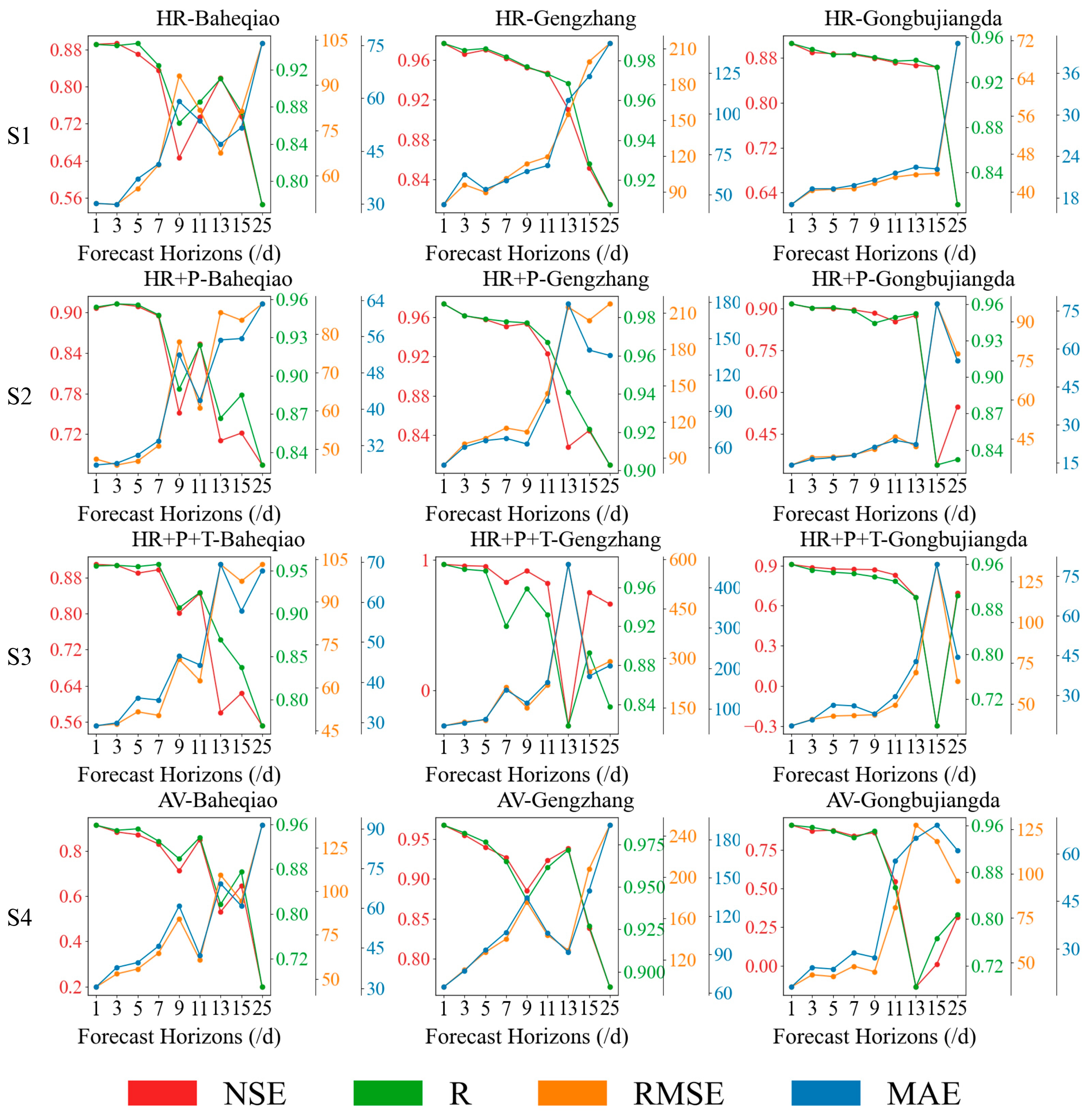
3.2. Model Prediction Results Under Different Forecasting Periods

The LSTM model considers the results of runoff prediction under different forecast periods at Baheqiao Station, Gengzhang Station, and Gongbujiangda Station with memory times of 1, 3, 5, 7, 9, 11, 13, and 15 days. The evaluation index values under different memory times are shown in

Table 4. Average prediction results of different foresight periods in the watershed.

Evaluation	Forecast Period 1 d	Forecast Period 3 d	Forecast Period 5 d	Forecast Period 7 d	Forecast Period 9 d	Forecast Period 11 d	Forecast Period 13 d	Forecast Period 15 d	Forecast Period 25 d
NSE	0.93	0.93	0.92	0.91	0.86	0.88	0.80	0.63	0.68
RMSE (m3/s)	55.58	61.89	63.89	68.21	77.00	83.50	114.27	128.12	127.69
MAE (m3/s)	29.13	35.01	37.55	39.49	45.41	54.81	85.40	91.26	84.83

, and the Taylor plot is shown in Figure 3.

From the Taylor diagram (Figure 3), it can be seen that the correlation coefficient of Gengzhang Station is higher than that of Baheqiao Station and Gongbujiangda Station under different forecast periods. Among them, the correlation coefficient results of schemes S1 and S2 are relatively close, higher than schemes S3 and S4. The magnitude of RMSE and MAE values varies among the three stations based on their catchment areas, but overall, the shorter the forecast period, the smaller the RMSE and MAE.

Taking Gengzhang Station as an example, the evaluation index values of various prediction schemes under different memory times are shown in Table 4. During the forecast period of 1–25 days, NSE decreased from 0.93 to 0.68, a decrease of 32%. RMSE increased from 55.58 m³/s to 127.69 m³/s, and MAE increased from 29.13 m³/s to 84.83 m³/s.

Figure 4 shows the prediction results of different prediction schemes under different forecast periods (red, green, orange, and blue correspond to NSE, R, RMSE, and MAE, respectively). Comparing the prediction effects of the three stations, it is found that the NSE at Gengzhang Station has the best performance at different prediction times. Comparing the simulation effects under different variables, the use of historical runoff and precipitation forecasts are the most stable, with an overall predicted NSE above 0.65.

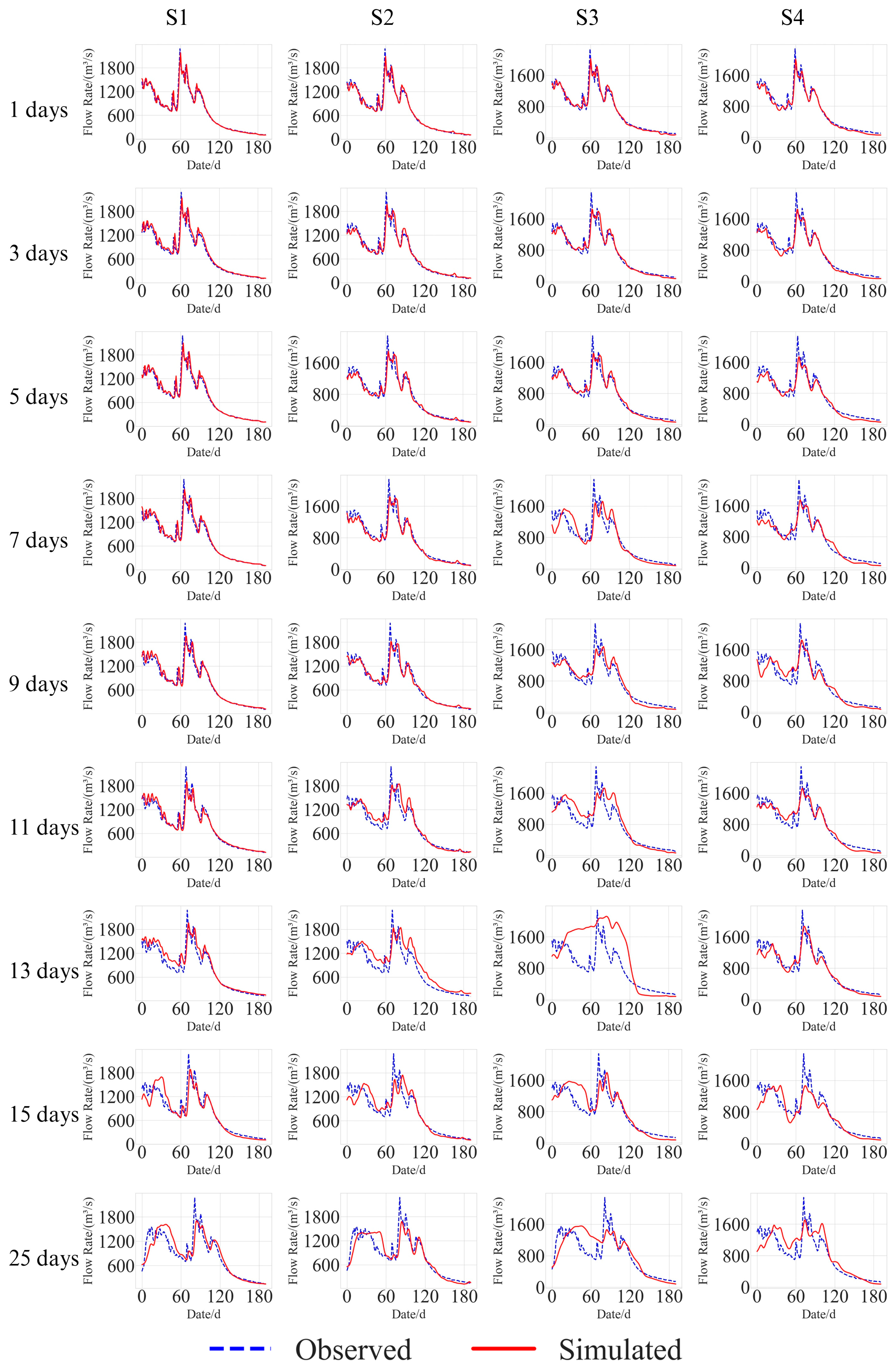
3.3. Simulation Effect of Runoff Under Different Forecasting Periods

To explore the impact of different forecast periods on the simulation effect of runoff processes, Figure 5 shows the simulation effect of runoff processes at Gengzhang Station under different forecast schemes. It can be seen that Scheme 1 has a relatively consistent simulation effect on runoff processes within the 9-day forecast period, Scheme 2 also has a good effect within the 9-day forecast period, but there is a slight bias in the simulation of high-value runoff areas. The prediction results of Scheme 3 and Scheme 4 are slightly worse than those of Scheme 1 and Scheme 2, and the simulated runoff and measured runoff effects within the 5-day forecast period are in good agreement. Scheme 3 has a smoothing effect on the simulation of runoff processes when the forecast period is higher than 5 days, and Scheme 4 has a high and low value simulation of runoff processes when the forecast period is higher than 4 days. There is a certain deviation in the simulation.

3.4. Contribution of Different Variables to Runoff Prediction

Grad CAM was used to analyze the contribution of variables to runoff prediction at different forecast times (Figure 6). From the perspective of the contribution of different variables to different forecast times, historical runoff has the greatest impact on runoff forecasting. As the forecast time increases, the contribution of historical runoff gradually decreases, and when the forecast time reaches 11 days or more, the contribution of historical runoff shows an upward trend. The prediction time is 1–5 days, and the contributions of temperature, and precipitation are relatively close. As the prediction time increases, the contributions of temperature also increase, reflecting the impact of temperature changes on the melting of ice and snow in the NRB runoff. When the prediction time exceeds 13 days, the contribution of precipitation increases, becoming the most significant factor affecting the runoff prediction effect, excluding historical runoff.

4. Discussion

4.1. Applicability of LSTM in High Mountain Watersheds

The complex terrain and lack of observational data in high-altitude watersheds such as the QTP greatly limit the application of hydrological models. With the continuous integration and development of 3S technology and computer technology, machine learning models have also been widely applied in runoff prediction. However, the application effect, mechanism, and parameter settings of using LSTM for runoff prediction in high-altitude watersheds such as the QTP, where data are scarce, are still not clear enough. This article takes the NRB on the QTP as the research object and selects the applicability of the LSTM model in high mountain basins. According to the results in Table 3, whether it is Gongbujiangda Station, Baheqiao Station, or Gengzhang Station, when the forecast period is 1–9 d, the NSE under all four schemes is greater than or equal to 0.65. Therefore, LSTM can effectively predict runoff transformation in high mountain watersheds. Similar studies conducted in the Lhasa River Basin and the Niyang River Basin have shown that the LSTM can not only be applied to runoff simulation in areas with scarce data but also improve the performance of runoff simulation in high-altitude regions [31]. Juan et al. [21] also conducted runoff prediction in the Three Rivers Source Area of the QTP and found that artificial neural network models can be successfully used to simulate and predict runoff changes in the QTP runoff process, mutually verifying each other.

4.2. The Impact of Different Variables on Runoff Simulation and Prediction

Comparing the effects of different variables on runoff prediction, the results are shown in Figure 6. Overall, historical runoff contributes the most. With the extension of the forecast period, the influence of temperature and precipitation on the prediction accuracy gradually increases, indicating that adding factors such as precipitation can enhance the prediction effect of runoff over a longer forecast period. Similar conclusions have also been drawn in the study of the Xiangjiang River Basin [32]. The combination of historical runoff and hydrometeorological variables can achieve good results in runoff forecasting.

In the hydrological and climatic variables, this article selected temperature, precipitation, and historical runoff, and the results are shown in Figure 6. When the forecast period is below 13 days, the impact of temperature on runoff prediction is higher than that of precipitation, and as the forecast period increases, the impact of temperature gradually increases. When the forecast period is above 13 days, the contribution of precipitation increases, becoming the factor that has the greatest impact on runoff prediction, excluding historical runoff. Similar results have also been shown in studies on the Xiangjiang River Basin and Ganjiang River Basin. When the forecast period is 1 day, the most important runoff prediction factor is historical runoff, and as the forecast period increases, the impact of precipitation becomes more significant [32,33]. As the forecast period extends, the impact of historical runoff on runoff prediction gradually decreases, while the impact of precipitation information on runoff prediction gradually increases [33].

Both precipitation and temperature make substantial contributions to runoff, especially in the case of a longer forecast period. Precipitation mainly has a direct impact on the generation and confluence of runoff, while temperature can indirectly affect runoff by influencing snowmelt and the phase state of precipitation [34,35]. Meanwhile, the degrees of influence of temperature and precipitation vary depending on the time and the length of the forecast period.

4.3. The Impact of the Forecast Period on Runoff Simulation and Prediction

As the forecast period increases, the effectiveness of runoff simulation and prediction gradually deteriorates (Figure 3 and Figure 4). As the forecast period increases, the simulation and prediction effects of runoff gradually deteriorate [30]. In the study, when the forecast period at Gengzhang Station is increased to 25 days, the Nash–Sutcliffe efficiency (NSE) remains above 0.65. Similar conclusions have also been drawn in other high mountain watersheds [36]. However, when the forecast period is extended to 2–3 days, the prediction accuracy of all schemes significantly decreases. In the study of the Haihe River Basin, the LSTM model achieved the best prediction performance at a time step of 1 day [37]. Li Wenjia et al. [38] demonstrated through experiments that the larger the interval between prediction times, the greater the error, and the longer the prediction time, the worse the fitting effect at the peak.

In addition, the forecast period is 1–7 days, and there is no significant difference in the runoff simulation effect under different watershed areas. However, as the forecast period increases, the runoff simulation effect of the three control stations decreases, and the largest area has the smallest decrease (Table 3). It can be seen that the larger the watershed area, the better the runoff prediction effect. In the study of the Ganjiang River Basin, the same results were also shown, with the increase in basin area, the accuracy of runoff prediction under different schemes improved [33].

4.4. The Limitations of the Study

Although the research results of this article can demonstrate the great potential of LSTM models in runoff in high-altitude watersheds, there are still some limitations.

The QTP is highly sensitive to meteorological conditions, and the impact of glaciers, snow, and permafrost on regional runoff is very complex. This paper only takes into account the impacts of temperature, precipitation, and historical runoff on the runoff simulation and prediction of the Niyang River Basin. Data such as snow cover, snowmelt, or glaciers have not been introduced. The impact of snow cover on runoff is mainly considered indirectly through the influence of temperature. Juan et al. [22] pointed out that the runoff changes in different basins of the Qinghai–Tibet Plateau and their responses to climate change are different. Due to the strong influence of climate warming, the sensitivity of runoff to temperature changes has increased. Zhang et al. [35] summarized previous studies and demonstrated that in systems dominated by snow and glaciers, the response of runoff to climate change is closely related to the acceleration of glacier melting. Starting from the seasonal changes in the runoff in the Niyang River Basin, Jin et al. [37] pointed out that the rise in temperature is not sufficient to affect the ablation of glaciers in the mountainous areas at the top of the basin. It mainly accelerates the ablation of snow cover. The increase in temperature in April and May causes a large amount of snow to melt, leading to the transformation of snowfall into rainfall in October. The changes in precipitation mainly affect the runoff from July, August to September. Therefore, snow cover data will be introduced in the next step of the research.

The LSTM model used in this article is relatively simple and has achieved satisfactory results, but there is still room for improvement. Different LSTM models can be considered for runoff prediction to achieve better prediction results. There is no conflict between traditional “process oriented” hydrological and physical models and “data oriented” machine learning models. It can be considered to combine the two, complement each other’s advantages, and improve the applicability of hydrological models in high-altitude watersheds such as the QTP, in order to enhance runoff simulation and prediction capabilities [39]. Based on LSTM and combined with SWAT, Khandelwal et al. [40] constructed a hydrological model to simulate runoff by linking weather driving factors with runoff, integrating hydrological physical processes into machine learning models to make runoff simulation more accurate. Okkan et al. [41] integrated machine learning models into the CRR model based on ANN and SVR models, calibrated all free parameters, and used machine learning to process various output variables, ultimately achieving good runoff simulation results.

5. Conclusions

The study selected the NRB on the QTP as the research area and used the LSTM model to analyze the prediction effects of different prediction schemes under different prediction periods. Grad-CAM was used to analyze the contribution of each variable under different prediction periods, and the following conclusions were drawn:

(1)

Under multiple prediction schemes, the runoff simulation effects and prediction accuracy of Gongbujiangda, Baheqiao, and Gengzhang stations were compared. Overall, the prediction effects of schemes 1 and 2 were relatively close, slightly higher than schemes 3 and 4, indicating that the historical runoff and the scheme containing historical runoff and precipitation had the most robust prediction effects.

(2)

In both scheme 1 and scheme 2, the forecast period for the three stations within 25 days still has a good forecasting effect. When the forecast period is 1 d, the prediction accuracy is the highest, and as the forecast period increases, the accuracy of the runoff prediction gradually deteriorates. The shorter the forecast period, the better the simulation and the prediction of runoff.

(3)

Comparing the prediction results of different stations, the station with the largest catchment area has a better prediction effect. As the catchment area increases, under different schemes, the average decline rate decreases with the extension of the forecast period. It can be seen that the larger the catchment area, the better the runoff prediction effect.

(4)

Comparing the runoff prediction effects of different variables, the overall historical runoff contributes the most. Among other variables, during the 1–5 day forecast period, the contribution of temperature and precipitation is relatively close. As the prediction time increases, the contribution of temperature increases, reflecting the impact of temperature changes on the melting of ice and snow in the NRB runoff. When the prediction time reaches 13 days or more, the contribution of precipitation increases, becoming the factor that affects the runoff prediction effect the most except for historical runoff. With the extension of the forecast period, the impact of temperature and precipitation on the prediction accuracy gradually increases, while the impact of historical runoff on runoff prediction gradually decreases compared to precipitation. When the forecast period reaches 13 days or more, the contribution of precipitation increases more significantly, indicating that adding factors such as precipitation and temperature can enhance the prediction effect of runoff over a longer forecast period.

References

1. Zolghadr-Asli, B.; Bozorg-Haddad, O.; Chu, X. Strategic Importance and Safety of Water Resources. J. Irrig. Drain. Eng. 2017, 143, 02517001. [Google Scholar] [CrossRef]
2. Li, P.; Yu, Z.; Jiang, P.; Wu, C. Spatiotemporal Characteristics of Regional Extreme Precipitation in Yangtze River Basin. J. Hydrol. 2021, 603, 126910. [Google Scholar] [CrossRef]
3. Zhou, Y.; Gui, Y.; Zhou, Q.; Li, L.; Chen, M.; Liu, Y. The Study on Spatial Distribution of Water Ecological Environment Carrying Capacity during Extreme Drought Conditions. Sci. Rep. 2024, 14, 11986. [Google Scholar] [CrossRef]
4. Ayzel, G.; Varentsova, N.; Erina, O.; Sokolov, D.; Kurochkina, L.; Moreydo, V. OpenForecast: The First Open-Source Operational Runoff Forecasting System in Russia. Water 2019, 11, 1546. [Google Scholar] [CrossRef]
5. Attar, N.F.; Sattari, M.T.; Apaydin, H. A Novel Stochastic Tree Model for Daily Streamflow Prediction Based on A Noise Suppression Hybridization Algorithm and Efficient Uncertainty Quantification. Water Resour. Manag. 2024, 38, 1943–1964. [Google Scholar] [CrossRef]
6. Arnold, J.G.; Moriasi, D.N.; Gassman, P.W.; Abbaspour, K.C.; White, M.J.; Srinivasan, R.; Santhi, C.; Harmel, R.D.; Van Griensven, A.; Van Liew, M.W.; et al. SWAT: Model Use, Calibration, and Validation. Trans. ASABE 2012, 55, 1491–1508. [Google Scholar] [CrossRef]
7. Mizumura, K. Runoff Prediction by Simple Tank Model Using Recession Curves. J. Hydraul. Eng. 1995, 121, 812–818. [Google Scholar] [CrossRef]
8. Simonov, Y.A.; Semenova, N.K.; Khristoforov, A.V. Short-Range Streamflow Forecasting of the Kama River Based on the HBV Model Application. Russ. Meteorol. Hydrol. 2021, 46, 388–395. [Google Scholar] [CrossRef]
9. Zhang, X.; Liu, P.; Cheng, L.; Xie, K.; Han, D.; Zhou, L. The Temporal Variations in Runoff-Generation Parameters of the Xinanjiang Model Due to Human Activities: A Case Study in the Upper Yangtze River Basin, China. J. Hydrol. Reg. Stud. 2021, 37, 100910. [Google Scholar] [CrossRef]
10. Mahanta, A.R.; Rawat, K.S.; Singh, S.K.; Baweja, H.S. Hydrological Simulation of Runoff for Stream Flow Prediction Using SWAT Model and GIS Techniques over Palar River Basin, India. AIP Conf. Proc. 2024, 3072, 040011. [Google Scholar]
11. Han, D.; Liu, P.; Xie, K.; Li, H.; Xia, Q.; Cheng, Q.; Wang, Y.; Yang, Z.; Zhang, Y.; Xia, J. An Attention-Based LSTM Model for Long-Term Runoff Forecasting and Factor Recognition. Environ. Res. Lett. 2023, 18, 024004. [Google Scholar] [CrossRef]
12. Islam, K.I.; Elias, E.; Carroll, K.C.; Brown, C. Exploring Random Forest Machine Learning and Remote Sensing Data for Streamflow Prediction: An Alternative Approach to a Process-Based Hydrologic Modeling in a Snowmelt-Driven Watershed. Remote Sens. 2023, 15, 3999. [Google Scholar] [CrossRef]
13. Samsudin, R.; Saad, P.; Shabri, A. River Flow Time Series Using Least Squares Support Vector Machines. Hydrol. Earth Syst. Sci. 2011, 15, 1835–1852. [Google Scholar] [CrossRef]
14. Taormina, R.; Chau, K.; Sethi, R. Artificial Neural Network Simulation of Hourly Groundwater Levels in a Coastal Aquifer System of the Venice Lagoon. Eng. Appl. Artif. Intell. 2012, 25, 1670–1676. [Google Scholar] [CrossRef]
15. Hussain, D.; Khan, A.A. Machine Learning Techniques for Monthly River Flow Forecasting of Hunza River, Pakistan. Earth Sci. Inform. 2020, 13, 939–949. [Google Scholar] [CrossRef]
16. Kumar, A.; Kumar, P.; Singh, V.K. Evaluating Different Machine Learning Models for Runoff and Suspended Sediment Simulation. Water Resour. Manag. 2019, 33, 1217–1231. [Google Scholar] [CrossRef]
17. Chen, Y.; Xu, J. Rainfall-Runoff Short-Term Forecasting Method Based on LSTM. J. Phys. Conf. Ser. 2021, 2025, 012005. [Google Scholar] [CrossRef]
18. Rahimzad, M.; Moghaddam Nia, A.; Zolfonoon, H.; Soltani, J.; Danandeh Mehr, A.; Kwon, H.-H. Performance Comparison of an LSTM-Based Deep Learning Model versus Conventional Machine Learning Algorithms for Streamflow Forecasting. Water Resour. Manag. 2021, 35, 4167–4187. [Google Scholar] [CrossRef]
19. Frank, C.; Rußwurm, M.; Fluixa-Sanmartin, J.; Tuia, D. Short-Term Runoff Forecasting in an Alpine Catchment with a Long Short-Term Memory Neural Network. Front. Water 2023, 5, 1126310. [Google Scholar] [CrossRef]
20. Cai, M.; Yang, S.; Zhao, C.; Zhou, Q.; Hou, L. Insight into Runoff Characteristics Using Hydrological Modeling in the Data-Scarce Southern Tibetan Plateau: Past, Present, and Future. PLoS ONE 2017, 12, e0176813. [Google Scholar] [CrossRef]
21. Chang, J.; Wang, G.; Mao, T.; Sun, X. ANN Model-Based Simulation of the Runoff Variation in Response to Climate Change on the Qinghai-Tibet Plateau, China. Adv. Meteorol. 2017, 2017, 9451802. [Google Scholar]
22. Huang, K.; Wang, G.; Song, C.; Yu, Q. Runoff simulation and prediction of a typical small watershed in permafrost region of the Qinghai-Tibet Plateau based on LSTM. J. Glaciol. Geocryol. 2021, 43, 1144–1156. (In Chinese) [Google Scholar]
23. Jing, X.; Luo, J.; Zhang, S.; Wei, N. Runoff Forecasting Model Based on Variational Mode Decomposition and Artificial Neural Networks. Math. Biosci. Eng. MBE 2021, 19, 1633–1648. [Google Scholar] [CrossRef]
24. Yuan, X.; Chen, C.; Lei, X.; Yuan, Y.; Adnan, R.M. Monthly Runoff Forecasting Based on LSTM–ALO Model. Stoch. Environ. Res. Risk Assess. 2018, 32, 2199–2212. [Google Scholar] [CrossRef]
25. Rizvi, S.A.; Tang, R.; Jiang, X.; Ma, X.; Hu, X. Local Contrastive Learning for Medical Image Recognition. arXiv 2023, arXiv:2303.14153. [Google Scholar]
26. Han, H.; Choi, C.; Jung, J.; Kim, H.S. Deep Learning with Long Short Term Memory Based Sequence-to-Sequence Model for Rainfall-Runoff Simulation. Water 2021, 13, 437. [Google Scholar] [CrossRef]
27. Zhang, J.; Yan, H. A Long Short-Term Components Neural Network Model with Data Augmentation for Daily Runoff Forecasting. J. Hydrol. 2023, 617, 128853. [Google Scholar] [CrossRef]
28. Selvaraju, R.R.; Cogswell, M.; Das, A.; Vedantam, R.; Parikh, D.; Batra, D. Grad-CAM: Visual Explanations from Deep Networks via Gradient-Based Localization. Int. J. Comput. Vis. 2020, 128, 336–359. [Google Scholar] [CrossRef]
29. Xiang, X.; Guo, S.; Cui, Z.; Wang, L.; Xu, C.-Y. Improving Flood Forecast Accuracy Based on Explainable Convolutional Neural Network by Grad-CAM Method. J. Hydrol. 2024, 642, 131867. [Google Scholar] [CrossRef]
30. Hu, Q.; Cao, S.; Yang, H.; Wang, Y.; Li, L.; Wang, L. Daily runoff predication using LSTM at the Ankang Station, Hanjing River. Prog. Geogr. 2020, 39, 636–642. (In Chinese) [Google Scholar] [CrossRef]
31. Yue, J.; Zhou, L.; Du, J.; Zhou, C.; Nimai, S.; Wu, L.; Ao, T. Runoff Simulation in Data-Scarce Alpine Regions: Comparative Analysis Based on LSTM and Physically Based Models. Water 2024, 16, 2161. [Google Scholar] [CrossRef]
32. Tian, Y.; Tan, W.; Wang, G.; Yuan, X. Application and interpretability of the LSTM models in runoff prediction. Water Resour. Prot. 2022, 1–13. (In Chinese) [Google Scholar]
33. Hu, L.; Jiang, X.; Zhou, J.; Ou, Y.; Dai, Y.; Zhang, L.; Fu, X. Application of LSTM considering time steps in runoff prediction of Ganjiang River Basin. J. Lake Sci. 2022, 36, 1–13. (In Chinese) [Google Scholar]
34. Zhang, M.; Ren, Q.; Wei, X.; Wang, J.; Yang, X.; Jiang, Z. Climate Change, Glacier Melting and Streamflow in the Niyang River Basin, Southeast Tibet, China. Ecohydrology 2011, 4, 288–298. [Google Scholar] [CrossRef]
35. Jin, H.; Ju, Q.; Yu, Z.; Hao, J.; Gu, H.; Gu, H.; Li, W. Simulation of Snowmelt Runoff and Sensitivity Analysis in the Nyang River Basin, Southeastern Qinghai-Tibetan Plateau, China. Nat. Hazards 2019, 99, 931–950. [Google Scholar] [CrossRef]
36. Zhang, Z.; Liu, S.; Ma, K.; Zhang, X.; Yang, Y.; Cui, F. Runoff simulation of the upper Jinsha River Basin based on LSTM driven by elevation dependent climatic forcing. Prog. Geogr. 2023, 42, 1139–1152. [Google Scholar] [CrossRef]
37. Zhang, Q.; Liu, W.; Chen, Z.; Hao, Y. Forecasting of river flow based on LSTM-SVM model. J. Tianjin Norm. Univ. (Nat. Sci. Ed.) 2023, 43, 45–52. (In Chinese) [Google Scholar]
38. Li, W.; Wu, L.; Wen, X.; Feng, Q.; Zhou, T.; Yang, L.; Yi, Z. Runoff simulation study based on LSTM-Seq2seq model optimized by Attention mechanism. J. Glaciol. Geocryol. 2023, 1–13. (In Chinese) [Google Scholar]
39. Wang, G.; Hao, X.; Yao, X.; Wang, J.; Li, H.; Chen, R.; Liu, Z. Simulations of Snowmelt Runoff in a High-Altitude Mountainous Area Based on Big Data and Machine Learning Models: Taking the Xiying River Basin as an Example. Remote Sens. 2023, 15, 1118. [Google Scholar] [CrossRef]
40. Khandelwal, A.; Xu, S.; Li, X.; Jia, X.; Stienbach, M.; Duffy, C.; Nieber, J.; Kumar, V. Physics Guided Machine Learning Methods for Hydrology. arXiv 2020, arXiv:2012.02854. [Google Scholar]
41. Okkan, U.; Ersoy, Z.B.; Ali Kumanlioglu, A.; Fistikoglu, O. Embedding Machine Learning Techniques into a Conceptual Model to Improve Monthly Runoff Simulation: A Nested Hybrid Rainfall-Runoff Modeling. J. Hydrol. 2021, 598, 126433. [Google Scholar] [CrossRef]
Figure 1. The terrain and distribution of river networks in the Nyang River Basin.
Water 17 01465 g001
Figure 2. Structure of LSTM model.
Water 17 01465 g002
Figure 3. Taylor plots of daily runoff simulation under different schemes.
Water 17 01465 g003
Figure 4. Prediction results of daily runoff simulations during different forecast periods.
Water 17 01465 g004
Figure 5. Simulation of runoff processes in different prediction schemes and forecast periods at Gengzhang Station.
Water 17 01465 g005
Figure 6. Contributions of various variables to runoff prediction (T: Temperature, P: Precipitation, HR: Historical Runoff).
Water 17 01465 g006