Spatial–Temporal Evolution of Agricultural Water Use Efficiency Based on DEA Approach and Spatial Autocorrelation

Abstract

With the change in climate and rapid social development, the problems of low agricultural water resource utilization efficiency (AWUE) and significant spatiotemporal variability in the Hebei Province of China are becoming increasingly prominent. This paper constructed a framework that considers environmental exogenous variables and selects evaluation indicators based on the Lasso model. It also used the Data Envelopment Analysis (DEA) model to measure AWUE from 2012 to 2021. Furthermore, the Global Moran’s Index (GMI) and Getis Ord Gi * Index (GOGI) were applied to explore characteristics and trends of the spatiotemporal of AWUE. The conclusions are as follows: (1) The AWUE showed a fluctuating development trend of first rising and then falling. However, it did not achieve the effectiveness of DEA in general, and AWUE still had the potential and room for improvement. (2) From the perspective of spatiotemporal variability of AWUE, the northeast region shows better performance than the southwest region. The AWUE among cities and areas had a significant but relatively loose spatial correlation. (3) From 2012 to 2021, the centroid distribution of AWUE hotspots showed a shift from central areas to northeast, with an average annual transfer distance of 11.14 km. In summary, this study emphasizes the urgent need to improve AWUE, which can provide a reference for water resources departments to formulate policy planning and management decisions tailored to local conditions.

1. Introduction

Hebei Province is an important grain and cotton production in China, covering 11 cities and areas, including Shijiazhuang, Tangshan, Qinhuangdao, Handan, and Xingtai, where population and GDP account for 5.26% and 3.5% of China, respectively. Known as the condensed national geography book, it has China’s most complete topography and ecosystem. However, the per capita water resources and the water resources per unit area of arable land in the basin are only 3.3% and 8.3% of the world average level, respectively [1]. Agricultural water consumption accounted for 70% of the groundwater water supply, and the effective utilization coefficient of agricultural irrigation water was about 0.679 [2]. Therefore, China put forward the “Action Plan for Comprehensive Control of Groundwater Over-exploitation in North China”, hoping to reduce water consumption and tap water saving potential so as to reduce agricultural water consumption and improve AWUE.

Water resource is an indispensable factor in agricultural production. In the process of crop growth, the abundance of water directly affects the quality and yield. At present, the shortage of water resources, inefficiency of water management, uneven temporal and spatial distribution of water resources, and extensive use of water have seriously restricted the sustainable development of agriculture in Hebei Province [3,4]. Therefore, studying the AWUE and its temporal and spatial differentiation in the Hebei Province of China under different conditions is conducive to speeding up the pace of regional agricultural modernization, breaking through the bottleneck of agricultural development caused by water scarcity, and providing support and guarantee for the sustainable development of the regional economy.

Scientific and accurate evaluation of water resource utilization efficiency is an important basis for promoting sustainable use of water resources and achieving the 2030 sustainable development goal of the United Nations. At present, many researchers study water resource utilization efficiency, mainly focusing on three aspects. The first aspect is the angle and method of evaluation of water resource utilization efficiency. In terms of the first aspect, from the perspective of angles, it is mainly divided into agricultural water resource utilization efficiency, industrial water resource utilization efficiency, urban domestic water resource utilization efficiency, comprehensive utilization efficiency of water resources, and so on. From the perspective of evaluation methods, they mainly include principal component analysis [5], analytic hierarchy process [6], projection pursuit method [7], stochastic frontier analysis [8], and data envelopment analysis [9]. In recent years, DEA has become more and more popular as a non-parametric method among academics because traditional measurement methods cannot overcome the shortcomings of complex cross-relationships among various factors and subjective weight assumptions in operation. Scholars from all over the country, such as Zhang et al. [10], Wang et al. [11], and Jo et al. [12], have used this method to study and evaluate the provincial water resources utilization efficiency in China, the environmental ecological efficiency in China, and the evaluation strategy of efficiency. Furthermore, AWUE was found to be the most prominent problem, especially in areas where groundwater over-exploitation is severe. Therefore, it is of great significance to select Hebei Province as the study area and conduct an AWUE evaluation of it from the perspective of agricultural water use using the DEA method.

The second aspect is the study of the factors of water resource utilization efficiency. Many scholars have mainly conducted research on the aspects of input–output, management mechanisms, policy measures, and so on. Wang et al. [11] evaluated the efficiency of water resource utilization based on DEA, considering multiple inputs and multiple outputs. Yao et al. [13] evaluated the water resource efficiency in the Beijing–Tianjin–Hebei region by taking into account the leakage rate of the water supply network, sewage treatment rate, and per capita daily water consumption. Shi et al. [14] considered precipitation as an environmental exogenous variable in the measurement of water resource utilization efficiency, and DEA is applied to evaluate the AWUE of the Yangtze River. Chang et al. [15] found that the level of water resource management and regional development are closely related to the efficiency of water resource utilization.

The third aspect is the research on the spatial and temporal differentiation of water resources utilization efficiency. Deng et al. [16] focus on the efficiency of water resource utilization in different departments as the research object and explore the spatiotemporal evolution mechanisms in Jiangsu Province. Charnes et al. [17], Zhu et al. [18], Shao et al. [19], and Cho et al. [20] mostly focus on static analysis of spatiotemporal changes in agricultural water resource efficiency in a certain region. In addition, the conventional spatial measurement method relying on “attribute data” limits the spatial relationship to geographically or economically adjacent regions, which only reveals some correlation relationships and lacks analysis of more complex network structure characteristics from a global perspective.

In summary, the research on water resource utilization efficiency has been relatively in-depth, and some achievements have also been made in AWUE based on the DEA model, but there is still some room for deepening. First, the research on the provincial level, where groundwater over-exploitation is still insufficient, is mostly concentrated on the national and comprehensive water resource efficiency evaluation [21,22,23]. Secondly, the existing water resource utilization efficiency evaluation methods are limited to considering the input and output indicators [24], and they have certain defects that cannot accurately evaluate the AWUE value. Finally, no dynamic analyses of the spatiotemporal changes in water resource utilization efficiency have been found [25,26].

Therefore, this paper first established an AWUE indicator screening framework through the Lasso model in order to evaluate AWUE more realistically. Then, under the conditions of climate change, the DEA model was employed to calculate the efficiency value of Hebei Province through panel data from 2012 to 2022 and carried out time series analysis. Finally, the GMI [27,28] and GOGI [29,30] are introduced, the AWUE of Hebei Province is quantified, and the spatial aggregation and distribution analysis is carried out. There are two contributions to this study. On the one hand, this paper adds precipitation and temperature as limiting conditions to evaluate the AWUE of each urban area in Hebei Province based on the traditional DEA model, which can enhance the authenticity and reliability of research results. On the other hand, this paper provides new ideas and perspectives for the existing literature, using The GMI and GOGI to analyze the spatial differentiation of AWUE from the perspectives of global and local correlations.

2. Study Area

Hebei Province is located in the North China Plain, bordering the Bohai Gulf in the east, Beijing and Tianjin in the inner ring, the Taihang Mountain in the west, the Yan Mountain in the north, and Zhangbei Plateau in the north of Yanshan Mountains (Figure 1a). With a temperate continental monsoon climate and distinct four seasons, the average annual precipitation of the Hebei Province decreases from 523 mm/year in the southeast to 403 mm/year in the northwest, with an annual average precipitation of 484.5 mm. Meanwhile, the average temperature in January is below 3 °C, and the average temperature in July is between 18 °C and 27 °C.

The total area of Hebei Province is 188,800 km², with complex and diverse landforms, including plateaus, mountains, hills, basins, and plains, among which the area of Hebei Plain geomorphic unit is 81,459 km², accounting for 43.15% of the total area, and the area of other geomorphic units is 107,341 km², accounting for 56.85% of the total area. The terrain is high in the northwest and low in the southeast, slopes from northwest to southeast. From 2012 to 2021, agricultural water consumption in Hebei Province accounted for 53–73% of the total water consumption; agricultural water consumption declined by 32%, from 14.3 billion m³ to 9.7 billion m³.

3. Materials and Methods

DEA is a common method for measuring AWUE, but there are still some disadvantages to using the traditional DEA model for measurement. First, the input–output indicators of the DEA model are generally considered to be commonly used factors in the literature, and climate factors are often not included as inputs. The second issue is that the DEA model does not qualitatively analyze the rationality of input–output indicators and cannot effectively solve the problem of negative values in input–output indicators. Thirdly, due to the inherent properties of the DEA model, the spatial variation characteristics of AWUE cannot be considered. Therefore, spatial autocorrelation is used to analyze AWUE.

Based on the above considerations, this study adopts a four-stage approach, proposes a hybrid technology, and considers climate change to comprehensively evaluate AWUE. In the first stage of data preparation, the input and output indexes of AWUE were determined based on the literature research. In the stage of evaluating the importance of indicators, the Lasso model is used to measure the relative importance of each element and further quantify the significance of the indicators. During the assessment stage of AWUE, Hebei Province’s AWUE from 2012 to 2021 was evaluated, while two scenarios were taken into account throughout the evaluation stage. In the fourth step, spatial autocorrelation analysis was employed to examine the clustering and spatiotemporal evolution features of AWUE over various periods. The methodological approach is illustrated in Figure 2.

3.1. Data Sources and Literature Review

From 2020 to 2024, a total of 74 articles were published in the AWUE field. By checking one by one, we further analyzed 16 articles closely related to this study, and on the basis of screening out 6 commonly evaluated indicators, 2 meteorological-related indicators were added. Six commonly evaluated indicators include gross agricultural output value (Y) [22,26], total sow area (S) [31,32], agricultural labor force (L) [17,33], total power of agricultural machinery (K) [33,34], consumption of chemical fertilizer (C) [35,36], and agricultural water consumption (W) [15,37]; the two meteorological indicators include preparation (P) [38,39] and temperature (T) [40,41,42,43], as shown in Figure 3.

Historical data on monthly average temperature and precipitation from 2012 to 2021 were provided by the China Meteorological Administration (http://www.nmic.cn/, accessed on 1 April 2025). Provincial crop area and statistical data, including Y, S, L, and K, etc., from the Hebei Statistical Year-book (https://www.stats.gov.cn/, accessed on 1 April 2025) and National Bureau of Statistics of China (http://www.hlj.stats.gov.cn/, accessed on 1 April 2025). Due to different natural conditions and economic development levels, agricultural production in Hebei Province has strong regional characteristics and is divided into eastern, northern, southern, and central regions. The input–output indicators are detailed in

Table 1. Input–output indicators system of agricultural water use efficiency.

Indicator	Symbol	Proxy Variables	Unit
Output indicators	Y	Gross agricultural output value	RMB
Land input	S	Total sown area	Hectares
Labor input	L	Agricultural labor force	People
Capital investment	K	Total power of agricultural machinery	Kilowatt
Material input	C	Consumption of chemical fertilizer	Tonnes
Agricultural water consumption input	W	Agricultural water consumption	Cubic meters
Precipitation input	P	Precipitation	mm
Temperature input	T	Temperature	°C

.

3.2. The Lasso Regression Model

Lasso regression is a processing method for solving the problem of intuitive collinearity and feature selection of indicators. Lasso regression transforms the loss function through the L1 regularization method. After cross-validation of the dataset, the regularized Lasso algorithm can select key indicators that have a significant impact on the research. The specific steps are as follows:

(1) Dataset processing:

$$D=(x_j,y_j)(j=1,2,\dots ,n)$$

(1)

x represents the explanatory variable, and y represents the dependent variable.

(2) Linear programming objective function:

$$\widehat{\beta }={arg}_{min}\left\{\sum _{j=1}^{\overline{n}}\left[{(y_j-\sum _{i=1}^{\overline{m}}\widehat{\beta }{x}_{ji})}^2+\lambda \sum _{i=1}^{\overline{m}}\left|{\beta }_i\right|\right]\right\}$$

(2)

$\widehat{\beta }$ is the constraint form of the minimum sum of squares, ${\sum }_{i=1}^{\overline{m}}\widehat{\beta }{x}_{ji}$ is the penalty term, and λ is the adjustment coefficient.

The regularized Lasso algorithm performs generalized cross-validation on the dataset to investigate the relationship between the harmonic parameter value λ and the model error. The harmonic parameter value λ automatically selected by the model is 0.06. Meanwhile, Pearson correlation analysis was used to test the correlation between input and output indicators. In this study, all statistical tests were conducted using the SPSS (V22.0) software.

3.3. Data Envelopment Analysis Model

DEA is based on linear programming and an efficiency evaluation method proposed by Charnes and Cooper (1978) [44]. In the process of efficiency evaluation, DEA measures the relative efficiency of decision-making units (DUMs) with consistent business objectives based on multiple observed input and output indicators. It has been widely used in many fields, such as production, management science, and economics [12,45].

There are various models for data envelopment analysis, including the CCR model, BBC model, crossover model, and so on, among which CCR and BBC are the most commonly used models [46,47]. The DEA-CCR assumes constant returns to scale and judges the relative rationality and effectiveness of each unit through an economic system that inputs a certain number of production factors and outputs a certain number of products; this model is called the input-oriented model. The DEA-BCC assumes that in the case of variable returns to scale when some decision-making units are not operating at the optimal scale, the measurement of technology efficiency (TE) will be influenced by scale efficiency (SE); this model is called the output-oriented model.

This study selects the cities in Hebei Province as the DMU. In period t, assume there are s DMUs, and the jth DMU, denoted as j = 1, 2, …, s, exhibits m inputs (x_1j, x_2j, …, x_mj) and n outputs (x_1j, x_2j, …, x_mj). It is important to note that if all inputs and outputs of the DMUs are strictly greater than 0, then the DEA-BCC model is

$$\left\{\begin{array}{l}\min [\theta -\epsilon ({\widehat{e}}^T{S}^{-}+e^T{S}^{+}\left)\right]\\ s.t.{\sum }_{j=1}^S{\lambda }_j{x}_{ij}+S^{-}=\theta x_0\\ {\sum }_{j=1}^S{\lambda }_j{y}_{ij}-S^{+}=\theta y_0\\ {\sum }_{j=1}^S{\lambda }_j=1\\ {\lambda }_j,S^{-}{,S}^{+}\ge 0,j=1,2,\dots ,S\end{array}\right.,$$

(3)

where θ is the effective value of the decision-making unit within a certain period of time; λ_j is the planned decision variable of the jth decision unit; ε is Archimedes’ infinitely small quantity; S⁻ and S⁺ are the input and desired output slack variable, respectively. θ_x0 and θ_y0 are the input and desired output values, respectively. x_ij represents the ith input element of the j decision-making unit, and y_ij represents the ith expected output of the j decision-making unit.

3.4. Spatial Autocorrelation Analysis Based on GMI and GOGI

3.4.1. Global Spatial Autocorrelation

Global spatial autocorrelation is commonly measured by the GMI [24,25,26], which can be used to estimate whether regional agricultural water consumption has a spatial correlation on the whole. The value range of GMI is between −1 and 1. A value greater than 0 shows a positive correlation, and the value of GMI closer to 1 implies that the distribution of agricultural water use has similar spatial clustering properties; that is, high values are adjacent to high values. A value less than 0 indicates a negative correlation, and the value of GMI closer to −1 indicates that the distribution of agricultural water use has a spatial aggregation of diverse features; that is, the high value is near the low value. The Global Moran’ I formula is

$$I={\displaystyle \frac{{\sum }_{i=1}^n{\sum }_{j=1}^n{w}_{ij}(x_i-\overline{x})(x_j-\overline{x})}{S^2{\sum }_{i=1}^n{\sum }_{j=1}^n{w}_{ij}}},$$

(4)

where x_i and x_j are the attribute values on the geographical units of region i and region j, respectively. $\overline{x}$ is the average value of attribute values in each region. The spatial weight matrix w_ij represents the proximity relationship between region i and region j. n is the number of measurement regions. S² is the sample variance.

3.4.2. Local Spatial Autocorrelation

Local spatial autocorrelation mainly reflects the degree of spatial aggregation of attribute variables within the local region; commonly used methods include Local Moran’ I and GOGI [17,33]. In this study, the G index method was utilized to identify the spatial distribution of hotspots in agricultural water consumption within the study area. The calculation formula for GOGI is shown in Equations (5)–(7):

$$G_i^{*}={\displaystyle \frac{{\sum }_{j=1}^n{w}_{i,j}{x}_j-\overline{X}{\sum }_{j=1}^n{w}_{i,j}}{S\sqrt{\frac{\left[n{\sum }_{j=1}^n{w}_{i,j}^2-{\left({\sum }_{j=1}^n{w}_{i,j}\right)}^2\right]}{n-1}}}},$$

(5)

$$\overline{X}={\displaystyle \frac{{\sum }_{j=1}^n{x}_j}{n}},$$

(6)

$$S=\sqrt{{\displaystyle \frac{{\sum }_{j=1}^n{x}_j^2}{n}}-{\left(\overline{X}\right)}^2}$$

(7)

where x_j is the attribute value of element j, w_i,j is the spatial weight between elements i and j, and n is the total number of elements.

4. Results and Discussion

4.1. Descriptive Statistics and Correlation Analysis of Input–Output Indicators

The survey dataset of the input–output indicates gross agricultural output value, total sown area, agricultural labor force, the total power of agricultural machinery, consumption of chemical fertilizer, agricultural water consumption, precipitation, and temperature in Hebei Province was analyzed in stages (2012–2017, 2018–2022). The descriptive statistics of each input–output indication are shown in

Table 2. Summary of input–output variables in macro aspect of Hebei Province.

Year	Variables	Mean	Standard	Coefficient	Min	10th	25th	50th	75th	90th	Max
			Deviation	Variation
2017–2012	Y	5,179,588	1,841,388	0.36	2,574,006	3,134,141	3,633,196	4,546,801	6,594,927	7,604,342	9,220,393
	S	760,201	307,479	0.40	190,086	366,188	455,617	790,095	1,001,133	1,108,306	1,207,825
	L	1,189,088	559,409	0.47	626,584	668,225	779,174	1,024,230	1,357,500	1,700,738	2,725,340
	K	6,919,309	5,194,505	0.75	290	1047	2,613,891	7,404,278	9,839,985	12,864,047	20,360,714
	C	286,365	136,692	0.48	100,283	108,290	140,110	291,890	429,412	472,825	487,732
	W	12	5	0.41	5	6	7	12	16	18	20
	P	550.61	90.24	0.16	391.91	426.24	488.53	552.04	612.48	680.11	742.35
	T	12.15	2.67	0.22	6.32	7.13	10.97	13.34	14.13	14.41	14.63
2021–2018	Y	3,613,351	2,751,687	0.76	91	500	221,881	3,988,795	5,695,937	6,996,701	9,764,508
	S	320,565	394,552	1.23	110	197	722	1053	686,247	954,173	1,095,623
	L	1,676,139	1,096,828	0.65	94,453	567,031	916,396	1,341,842	2,499,099	3,492,980	3,928,995
	K	3,052,876	4,046,765	1.33	104	176	806	1311	7,410,765	9,728,382	12,833,239
	C	120,381	151,987	1.26	6	10	25	41	283,681	347,252	438,829
	W	9	4	0.49	2	2	5	9	12	14	17
	P	528.89	102.33	354.31	0.19	406.58	456.69	508.07	582.06	679.62	783.68
	T	11.77	2.68	5.13	0.23	6.99	10.65	12.90	13.81	14.14	14.65

.

From 2012 to 2021, the gross agricultural output value of the output indicator was in a state of fluctuating growth, ranging from 45.3 to 57.4 million yuan, and the gross agricultural output value reached the maximum value in 2016, with an overall increase except for 2017 and 2019. On the other hand, the total sown area, agricultural labor force, total power of agricultural machinery, consumption of chemical fertilizer, agricultural water consumption, precipitation and temperature of the selected input indexes are 613,521–786,640 hectares, 10.01–12.23 million people, 0.591–0.992 million kilowatt, 22.36–29.89 thousand tons, 7–12 billion m³, 354.31–783.68 mm and 6.32–14.65 °C, respectively, with an overall situation is in a state of declining volatility.

Interestingly, from 2012 to 2017, the gross agricultural output value, total sown area, agricultural labor force, consumption of chemical fertilizer, gross agricultural output value, agricultural labor force, agricultural water consumption, and agricultural water consumption showed low variation coefficient (<0.5), while some input indicators showed a high coefficient of variation, with coefficients of variation higher than 1, for example, the total power of agricultural machinery (Table 2). From 2018 to 2022, the coefficient of variation in the gross agricultural output value, total sown area, agricultural labor force, consumption of chemical fertilizer, gross agricultural output value, agricultural labor force, agricultural water consumption, and total power of agricultural machinery is relatively high (>1), while the coefficient of variation in some input indicators is lower than 0.5, such as agricultural water consumption (Table 2). From 2012–2017 to 2018–2022, the input–output indicators’ coefficient of variation progressively rose, indicating an increase in data dispersion as well as more notable individual variances and volatility.

To better analyze the impact of input–output indicators on agricultural water use efficiency, the potential impact of input–output indicators on AWUE. In this study, the Pearson correlation analysis was used to test the correlation relationship between input and output indicators, as shown in Figure 4. There is a strong correlation between input and output index, and each correlation coefficient is statistically significant. This indicates that input indicators have a significant impact on output indicators to a large extent. During 2012–2017, input–output indexes basically showed a positive correlation, with correlation coefficients ranging from 0.20 to 1.00, while precipitation indicators were generally negative correlation with other indicators, with correlation coefficients ranging from −0.016 to −0.080. There is a strong positive correlation between agricultural water consumption and consumption of chemical fertilizer and gross agricultural output value, with the correlation coefficients reaching 0.87 and 0.89, respectively. During 2018–2022, the correlation between agricultural water consumption and consumption of chemical fertilizer and gross agricultural output value weakened, with correlation coefficients of 0.63 and 0.56, respectively. However, the correlation between the agricultural labor force and total power of agricultural machinery and consumption of chemical fertilizers became stronger, with correlation coefficients of 0.95 and 0.96, respectively.

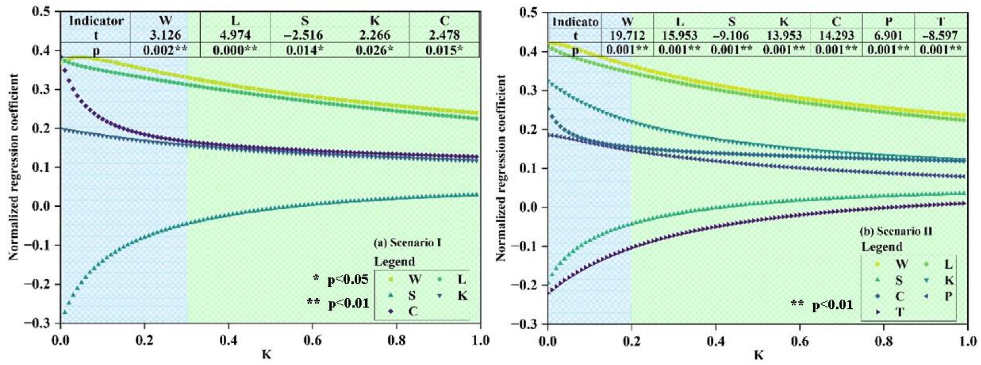
4.2. Determined the Indicators of AWUE Based on the Lasso Model

Firstly, when climate factors are not addressed, the ridge regression coefficient (k) is first derived based on the Lasso regression model by adding the unit matrix and combining it with the track diagram. In this scenario, k is 0.30. Generally, the smaller the k value, the less the deviation. Secondly, the Lasso model was run with the k value entered. The assessment results revealed that the model’s R² was 0.685, meaning that W, L. S, K, and C could account for 68.50% of the variations in Y. Figure 5a shows that the regression coefficients for W is 14.84 (t = 3.126, p = 0.002 < 0.01), L is 0.891 (t = 4.974, p = 0.000 < 0.01), and S is −1.457 (t = −2.516, p = 0.014 < 0.05). The regression coefficients for K (t = 2.266, p = 0.026 < 0.05) and C (t = 2.478, p = 0.015 < 0.05) were 0.070 and 4.437, respectively. Overall, W, L, K, and C have a considerable positive influence on Y, but S has a significant negative impact.

When considering climate factors, the track diagram shows k as 0.1, and the evaluation result of the Lasso model shows R² as 0.728, indicating that adding climate factors can explain 72.8% of the change in Y. Therefore, by comparing scenarios without considering climate factors, climate factors are also important factors driving Y. As shown in Figure 5b, the regression coefficient of W is 16.32 (t = 19.712, p = 0.000 < 0.01), L is 0.972 (t = 15.953, p = 0.000 < 0.01), K is 0.114 (t = 13.953, p = 0.000 < 0.01), C is 2.922 (t = 14.293, p = 0.000 < 0.01), P is 34.62 (t = 6.901, p = 0.000 < 0.01), S is −0.931 (t = −9.106, p = 0.000 < 0.01), and T is −14.56 (t = −8.597, p = 0.000 < 0.01). Overall, W, L. K, C, and P have a significant positive impact on Y, while S and T have a significant negative impact on Y.

4.3. AWUE Evaluation Analysis Based on DAE from the Time Scale

Through a literature review and Lasso model analysis, the input indicators of the DEA model were screened and subjected to regression analysis. The selected indicators were utilized as inputs to the DEA model, which was used to assess the AWUE of several cities in Hebei Province from 2012 to 2021. From Figure 6a, the AWUE of the east area in Hebei displayed strong efficiency because Tangshan and Qinhuangdao all maintain a high AWUE of greater than 0.9. Central Hebei and South Hebei, specifically Baoding and Xingtai, maintained a low AWUE for a long time. In north Hebei, Chengde and Zhangjiakou have weak AWUEs. From a provincial perspective, the overall trend of AWUE shows a decreasing gradient from northeast to south and central.

The Hebei Province classifies 11 cities into four categories: north, central, south, and east, according to geography. From Figure 6, we found that there were several AWUE trends at the municipal and regional levels. From a regional level (Figure 6a), the AWUE in the region from high to low levels was as follows: East Hebei, North Hebei, Central Hebei, and South Hebei. From 2015 to 2021, many regions experienced a reversal in AWUEs. At this time, the AWUE in three regions, including North Hebei, Central Hebei, and South Hebei, showed a downward trend, while the AWUE in East Hebei showed a downward trend. At the municipal level (Figure 6d), the cities in Esat Hebei and North Hebei, for example, Tangshan, Qinhuangdao, Zhangjiakou, and Chengde, maintain high AWUE levels. The cities in South Hebei and Central Hebei maintained their AWUE at a low level. The developed cities, such as Shijiazhuang, Cangzhou, and Langfang, in the central Hebei regions had higher AWUE values than Baoding and Hengshui. So, municipalities in the north and east regions had a high AWUE level, which is easier in mountainous and humid areas.

Province-wide (Figure 6b) and municipal-level AWUEs were divided into three parts. The first group concentrated at a high level from 2012 to 2017, the second group concentrated at a moderate level from around 2012 to 2017, and the third group concentrated at a low level from 2017 to 2021. In the northeast, the density of AWUE ranges from 0.52 to 0.68, which means that there were few cities at this level. In other words, the AWUE of Hebei Province has been at a relatively low level since 2017. Therefore, promoting agricultural development and agricultural water use management in Hebei Province requires more investment in labor and funds. As shown in Figure 6c, there are significant spatial differences in AWUE. From the perspective of Technical Pure Technical Efficiency (PTE) and Efficiency (TE), it can be seen that the corresponding axes of Handan, Xingtai, and Cangzhou in the radar map are significantly shorter than those of other cities. Meanwhile, from the perspective of scale efficiency (SE), the axes of Langfang and Cangzhou in the radar map are obviously shorter than those of other cities. The PTE of Shijiazhuang, Tangshan, and Baoding is higher than that of other cities. Based on actual data, the total agricultural output value in Shijiazhuang, Tangshan, and Baoding is significantly higher than in other cities, indicating that these cities have a higher level of agricultural water management and technology.

4.4. AWUE Autocorrelation Analysis Based on GMI and GOGI from the Spatial Scale

4.4.1. Global Spatial Autocorrelation Analysis of AWUE

According to the DEA model calculation results, the range of AWUE is between 0 and 1. In order to analyze the AWUE in Hebei Province, this article divided the range of AWUE into five parts, namely [0.52–0.62], [0.62–0.72], [0.72–0.86], [0.86–0.90], [0.90–1.00], and divides them into the lowest, low, medium, high, and highest levels according to color. This study visualized AWUE using ArcGIS 10.4 software (Figure 3) to analyze the spatial situations at the municipal and regional levels. As shown in Figure 7, cities with high AWUE levels are mainly distributed in the eastern and northern regions. However, the AWUE in the southern region is at a low level. In addition, the AWUE in the central region shows an unstable phenomenon.

The spatial autocorrelation analysis tool of ArcGIS software was used to calculate the Global Moran’ I in the four periods from 2012 to 2014, from 2014 to 2016, from 2017 to 2019, and from 2021 to 2021. The Global spatial autocorrelation results of AWUE are presented in

Table 3. Global Moran’ I value of the agricultural water use efficiency.

Value	2012–2014	2015–2016	2017–2019	2020–2021
Global Moran’ I	0.841	0.832	0.826	0.813
Z-Score	9.350	9.260	9.188	9.032
P	0.030	0.045	0.045	0.060

. Overall, the Global Moran index gradually decreases over time, which indicates an increasing spatial difference in AWUE. As shown in Table 3, the global spatial correlation of AWUE is effective. The Global Moran index value of AWUE were 0.841, 0.832, 0.826, and 0.813 in four periods; the spatial clustering index values were 9.350, 9.260, 9.188, and 9.032 in four periods; and the significance values were 0.030, 0.045, 0.045, and 0.060 in four periods, respectively.

These results indicate a positive spatial correlation between the agricultural water use efficiency of the 11 prefecture-level cities in Hebei Province as spatial units. It suggests the presence of spatial difference phenomenon in AWUE. There are several reasons that lead to significantly increased spatial differences. First, the severe regional or municipal economic gap has led to a large difference in research and development expenditures, which widened the discrepancy AWUE in various cities. Second, the developed cities of AWUEs far exceed the undeveloped cities. Third, due to the 11 cities in Hebei Province located in different locations, there are significant differences in the inputs of the DEA model, including gross agricultural output value, total soft area, agricultural labor force, the total power of agricultural machinery, consumption of chemical fertilizer, agricultural water consumption, precipitation, and temperature. Therefore, the AWUE in the eastern and northern regions can be maintained at a higher level than in the central and southern regions.

4.4.2. Local Spatial Autocorrelation Analysis of AWUE

In order to identify the spatial distribution of AWUE in Hebei Province, this study adopted ArcGIS spatial statistical analysis tool clustering and the Getis Ord Gi* analysis method to clarify the spatial correlation degree among cities. Secondly, the natural breakpoint classification method was used to divide spatial clustering into five categories: cold spot area, sub-cold area, warm spot area, sub-hot area, and hot spot area. Figure 8 shows the spatial clustering of AWUE at the municipal level in Hebei Province during 2012–2014, 2015–2016, 2017–2019, and 2020–2021.

The results of local autocorrelation analysis (Figure 8) indicate that in 2012–2014, there was a concentration of hot spots in Shijiazhuang, Chengde, Qinhuangdao, and Tangshan located in the southwest and northeast regions of the study area. Conversely, cold spots were concentrated in Baoding and Zhangjiakou in the western part of the study area. In 2015–2016, hot spots concentrated in Shijiazhuang and Tangshan. In 2017–2019, hot spots remained concentrated in Shijiazhuang, Chengde, Qinhuangdao, and Tangshan within the southwest and northeast regions while expanding to include Cangzhou and Hengshui. Cold spots continued to be concentrated in Baoding and Zhangjiakou but expanded to encompass Xingtai, which was located towards the west. Looking ahead to 2020–2021, it is anticipated that hot spots will remain concentrated in Shijiazhuang, Chengde, Qinhuangdao, and Tangshan within the southwest and northeast regions of the study area. Conversely, cold spots will continue to be concentrated in Baoding, Xingtai, and Zhangjiakou, which are located to the west of the study area.

On the whole, the agricultural water use efficiency in Hebei Province exhibits a significant spatial pattern of north–south disparity, primarily influenced by natural geographical conditions and agricultural production circumstances. The northeastern region of Hebei Province demonstrates a high level of agricultural modernization, with Tangshan, Qinhuangdao, and Chengde serving as prominent regional clusters. This is mainly attributed to their effective utilization of agricultural water resources, wherein they achieve higher agricultural water use efficiency while maintaining a certain level of agricultural output. Conversely, the western region of Hebei Province displays lower levels of agricultural modernization, with Xingtai, Baoding, and Zhangjiakou acting as cold-spot regional clustering centers. These areas face water resource scarcity, resulting in limited agricultural water consumption and insufficient awareness regarding water conservation practices. Consequently, there is an inability to effectively utilize available agricultural water resources or improve overall water use efficiency compared to other regions. As a result, the spatial correlation effect continues to strengthen while maintaining a highly stable distribution pattern.

4.5. Evolution Trend and Direction Analysis of AWUE

To quantitatively analyze the direction and magnitude of the overall trend in the distribution of hot spots for agricultural water resource use efficiency in the study area, ArcGIS was utilized to calculate both centroid and standard deviation ellipse values for each year’s hot spot data (Figure 9). The resulting changes in these values were then compiled into

Table 4. Change in hotspots centroid and standard deviation ellipse.

Year	Type	Longitude (°)	Latitude (°)	Rotation Angle (°)	Displacement (km)
2012–2014	Efficiency value	117.521	39.494	44.92	-
2015–2016	Efficiency value	117.201	39.634	20.51	49.85
2017–2019	Efficiency value	118.071	39.944	37.74	26.34
2020–2021	Efficiency value	118.356	40.392	136.46	35.24

.

The center of mass of the high-value area of agricultural water use efficiency in the study area generally shifted from the middle to the northeast (Figure 9). In 2012–2014, the centroid of hot spots was located in the middle of the Hebei plain, and the standard deviation ellipse almost covered a line extending from southeast to northeast. During this period, agricultural water resource utilization efficiency exhibited a strong directional and wide distribution pattern.

From 2015 to 2016, the centroid of hot spots was located in Tangshan of Hebei Plain. As shown in Table 4, by 2017, the focal point had moved approximately 49.85 km towards the northeast, significantly reducing its range. This indicates that during this period, the high-value area for agricultural water resource utilization efficiency remained primarily concentrated in the northeastern region, where significant improvements were observed. In 2020–2021, there was a further shift of approximately 26.34 km towards the northeast for hot spot centroid related to agricultural water resource utilization efficiency, consequently narrowing down its range even more significantly. This suggests that during this period, the high-value area for agricultural water resource utilization efficiency was mainly confined to the northeastern corner of our study area.

5. Conclusions

Under the precondition of precipitation and temperature as exogenous variables, the AWUE of 11 cities and areas in the Hebei province from 2012 to 2021 are calculated by the DEA model, and the change characteristics are analyzed. Then, the GMI and GOGI were used to obtain the evolution trend of the spatial-temporal dimension of AWUE. The conclusions are as follows:

(1)

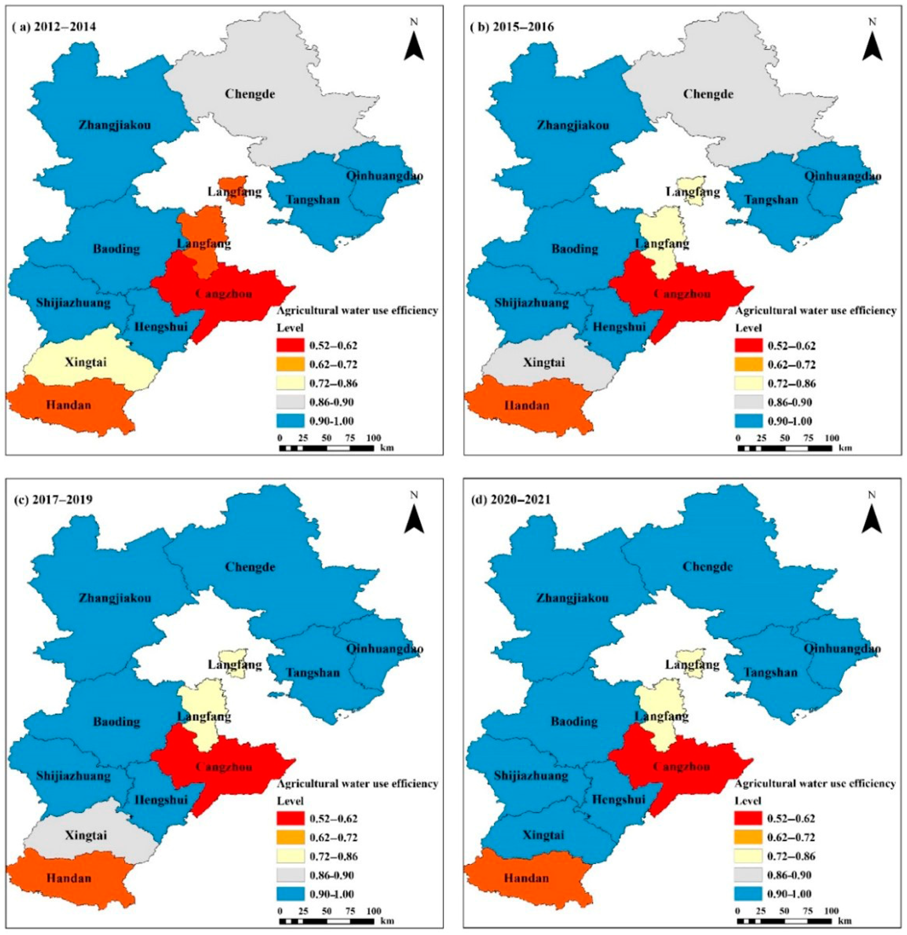
On the whole, under the changing environment from 2012 to 2021, the AWUE of the Hebei Province did not reach DEA effectiveness, and the average overall efficiency was 0.828, indicating that the AWUE still has potential and room for improvement. Among them, the annual average of AWUE in the southwest region is lower than 0.8, which are invalid DEA cities that need to be improved. The average AWUE of the northeast region is between 0.77 and 0.91, which is a strong EDA efficiency.

(2)

From the dynamic trend, the average value of each region of AWUE in the Hebei Province shows a fluctuating development trend of first rising, then falling, and then rising with time under the changing environment during the study period. AWUE reached the maximum in the window period 2014–2016.

(3)

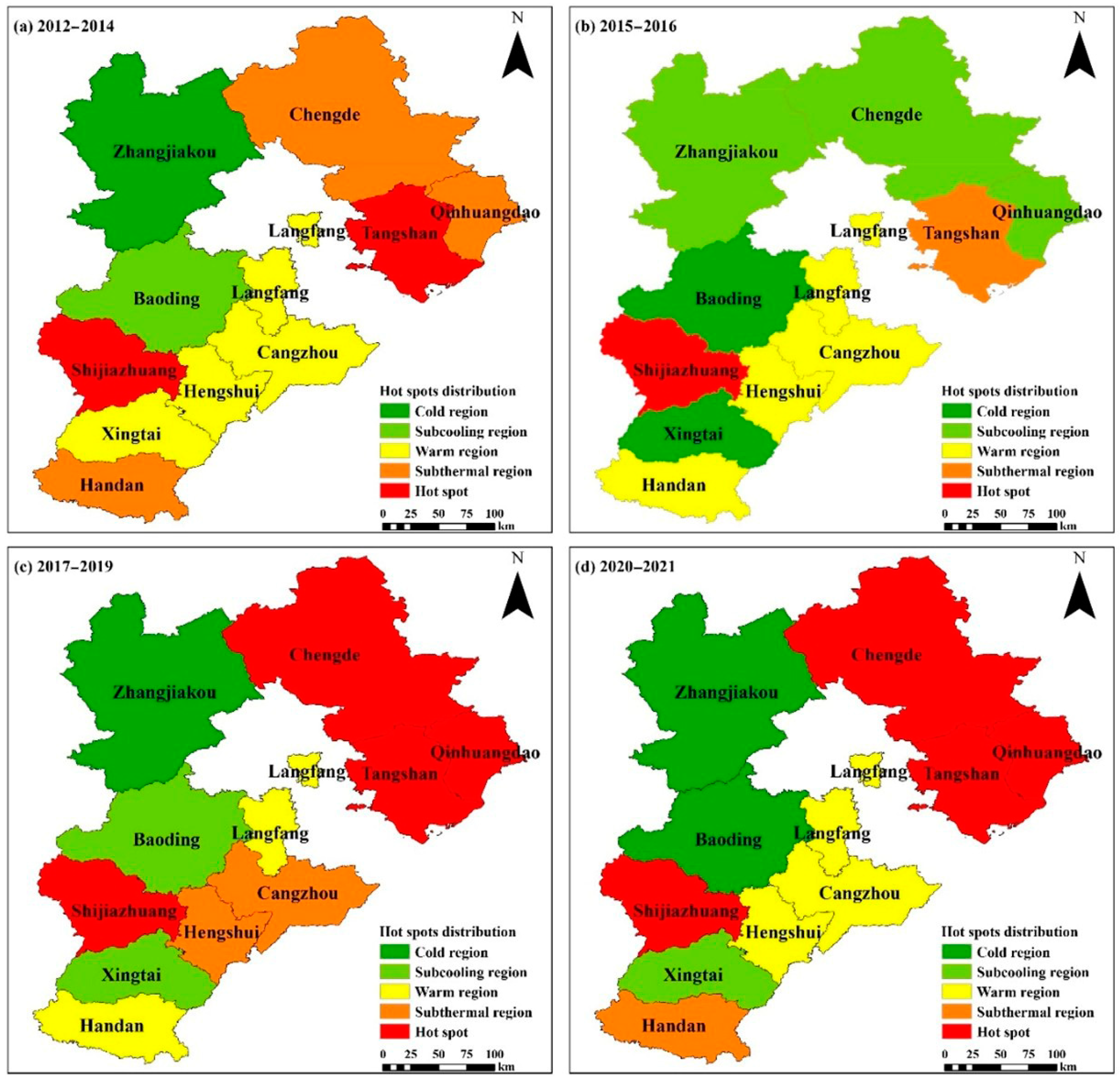
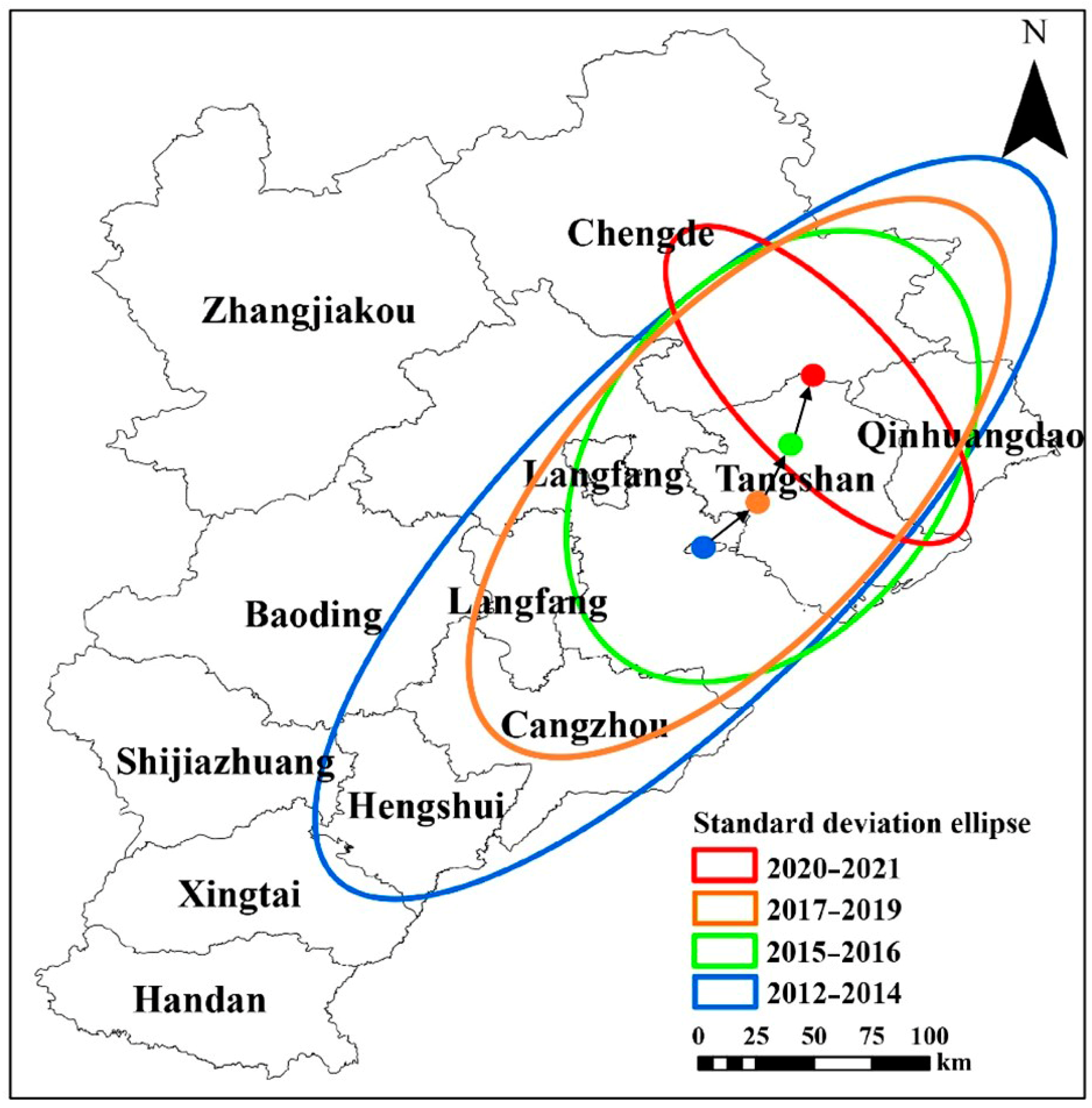
The distribution of AWUE shows a directional pattern from southwest to northeast. The AWUE in the southwest region has always been low, while the efficiency of agricultural water use in the northeast region has always been a high-value area, with the center of gravity gradually shifting towards the northeast from 2012 to 2021. The results of the hotspot centroid and standard deviation ellipse further indicate that attention should be paid to improving AWUE in the southwest region.

References

1. Qi, H.; Dong, Z.L.; You, X.S.; Li, Y.; Zhao, Y.R.; Sun, X.T. Extended exergy accounting for assessing the sustainability of agriculture: A case study of Hebei Province, China. Ecol. Indic. 2023, 150, 110240. [Google Scholar] [CrossRef]
2. Liu, S.Y.; Wu, X.D.; Han, M.Y.; Zhang, J.J.; Chen, B.; Wu, X.F.; Wei, W.D.; Li, Z. A three-scale input-output analysis of water use in a regional economy: Hebei province in China. J. Clean. Prod. 2017, 156, 962–974. [Google Scholar] [CrossRef]
3. Liu, T.X.; Zhang, D.S.; Shi, Y.F.; Li, Y.; Sun, J.C.; Zhang, X.P. The Influence of the South-to-North Water-Diversion Project on Terrestrial Water-Storage Changes in Hebei Province. Water 2023, 15, 3112. [Google Scholar] [CrossRef]
4. Li, S.L.; Yan, J.J.; Pei, Q.M.; Sha, J.H.; Liu, F. Dynamic Relationship Between Water Resources and New Urbanization Based on a Vector Autoregressive Model: A Case Study of Hebei Province, China. Front. Environ. Sci. 2022, 10, 941726. [Google Scholar] [CrossRef]
5. Li, Y.G.; Sun, M.H.; Yuan, G.H.; Liu, Y.J. Evaluation methods of water environment safety and their application to the three northeast provinces of China. Sustainability 2019, 11, 5135. [Google Scholar] [CrossRef]
6. Yang, G.S.; Xie, Q.H. Study on spatial and temporal differentiation of green water resource efficiency in the YREB. Resour. Environ. Yangtze Basin 2019, 28, 349–358. [Google Scholar]
7. Zhang, X.D.; Zhu, S. Spatial differences and influencing factors of regional agricultural water resource utilization efficiency in Heilongjiang Province China. Water Supply 2019, 19, 545–552. [Google Scholar]
8. Song, J.F.; Chen, X.N. Eco-efficiency of grain production in China based on water footprints: A stochastic frontier approach. J. Clean. Prod. 2019, 236, 117685. [Google Scholar] [CrossRef]
9. Zhou, Y.W. Utilization efficiency and influencing factors of agricultural water resource in Hubei province. Desalination Water Treat. 2019, 168, 201–206. [Google Scholar] [CrossRef]
10. Zhang, X.; Lin, Z. Evaluation of water resource utilization efficiency in provincial areas of China based on the unexpected output SBM model. J. Environ. Public Health 2022, 2022, 9554730. [Google Scholar] [CrossRef]
11. Wang, Q.; Wang, S. The impact of environmental regulation on water resources utilization efficiency. Front. Environ. Sci. 2022, 10, 1022929. [Google Scholar] [CrossRef]
12. Jo, J.; Kim, S. Assessing shoring strategies based on efficiency. Expert Syst. Appl. 2022, 207, 118032. [Google Scholar] [CrossRef]
13. Yao, T.; Liu, S. Comparison of the variation characteristics of water resource use efficiency indicators in the Beijing-Tianjin-Hebei region. Adv. Earth Sci. 2021, 36, 1195–1207. [Google Scholar] [CrossRef]
14. Shi, C.F.; Li, L.J.; Chiu, Y.H.; Pang, Q.H.; Zeng, X.Y. Spatial differentiation of agricultural water resource utilization 508 efficiency in the Yangtze River Economic Belt under changing environment. J. Clean. Prod. 2022, 346, 131200. [Google Scholar] [CrossRef]
15. Chang, M.; Chen, S.B.; Ma, B.R.; Liu, Y. Analysis of grain water resources utilization efficiency and influencing factors: An empirical study based on China’s provincial panel data. J. Ecol. Rural Environ. 2020, 36, 145–151. [Google Scholar]
16. Deng, M.H.; Zhang, T.S. Spatial-temporal evolution of water resources utilization efficiency in Jiangsu province. Water Supply 2023, 23, 2539–2552. [Google Scholar] [CrossRef]
17. Charnes, A.; Clark, C.T.; Cooper, W.W. A developmental study of data envelopment analysis in measuring the efficiency of maintenance units in the U.S. Air forces. Ann. Oper. Ann. Oper. Res. 1983, 2, 95–112. [Google Scholar] [CrossRef]
18. Zhu, D.; Tang, L.; Xie, Q.W.; Ma, M.; Rao, K.F. Efficiency assessment of water resource utilization cities based on data envelopment analysis. Acta Ecol. Sin. 2020, 40, 1956–1966. [Google Scholar]
19. Shao, L.G.; Yu, X.; Feng, C. Evaluating the eco-efficiency of China’s industrial sectors: A two-stage network data envelopment analysis. J. Environ. Manag. 2019, 247, 551–560. [Google Scholar] [CrossRef]
20. Cho, I.; Heo, E.; Park, J. Water resource R&D efficiency in Korea-toward sustainable integrated water resource management. Water Policy 2021, 23, 581–598. [Google Scholar]
21. Wang, X.X.; Cui, B.L.; Chen, Y.N.; Feng, T.; Li, Z.; Fang, G.H. Dynamic changes in water resources and comprehensive assessment of water resource utilization efficiency in the Aral Sea basin, Central Asia. J. Environ. Manag. 2024, 351, 120198. [Google Scholar] [CrossRef] [PubMed]
22. Ji, L.; Tao, S.G.; Liu, J.W.; Sun, Y.N.; Chiu, Y.H. Assessing the Efficiency of Industrial Water Use and Wastewater Treatment Across Provinces in China After Considering the Impact of Precipitation. Water Econ. Policy 2025. [Google Scholar] [CrossRef]
23. Zhou, Z.X.; Li, M.Y.; Xu, X.Z.; Wu, H.Q. Integrating spatial relationships in the DEA approach for ecological efficiency evaluation: A case study of the Chaohu watershed. Ecol. Indic. 2024, 169, 112868. [Google Scholar] [CrossRef]
24. Quan, Z.M.; Zuo, Q.T.; Zang, C.; Wu, Q.S. A multi-index comprehensive evaluation method for assessing the water use balance between economic society and ecology considering efficiency-development-health-harmony. Sci. Rep. 2024, 14, 25924. [Google Scholar] [CrossRef]
25. Sun, L.; Zhang, C.; Liu, Q.C.; Xu, C.X.; Song, M. Spatiotemporal evolution and optimization analysis of investment efficiency in China’s agricultural water conservancy infrastructure based on a two-stage DEA model. Front. Earth Sci. 2024, 12, 145535. [Google Scholar] [CrossRef]
26. Yin, C.J.; See, K.F.; Hsiao, B. Assessing the performance of water supply operations in Chinese water companies: A union dynamic multi-activity network data envelopment analysis. J. Clean. Prod. 2024, 482, 143750. [Google Scholar] [CrossRef]
27. Zhou, C. COVID-19: Challenges to GIS with big data. Geogr. Sustain. 2020, 1, 77–87. [Google Scholar] [CrossRef]
28. Yang, W.P.; Zhang, Z.Y.; Luo, P.P.; Wang, Y.J. Temporal and spatial evolution and influencing factors of urban ecological total factor productivity in the Yellow River basin under strong sustainable development. Sci. Prog. 2023, 106, 8504. [Google Scholar] [CrossRef]
29. Wu, Y.P.; Du, B.H.; Xu, C.Y.; Wei, S.B.; Yang, J.H.; Zhao, Y.P. Research on the Temporal and Spatial Distribution of Marginal Abatement Costs of Carbon Emissions in the Logistics Industry and Its Influencing Factors. Sustainability 2025, 17, 2839. [Google Scholar] [CrossRef]
30. Zhang, Y.P.; Wang, M.X. Spatio-temporal evolution characteristics and influencing factors of environmental welfare performance in Chinese cities. Front. Public Health 2025, 13, 1543745. [Google Scholar] [CrossRef]
31. Lv, T.G.; Li, Z.Y.; Zhang, X.M.; Geng, C.; Hu, H.; Xiao, J. Spatial-Temporal Differences and Influencing Factors of Agricultural Water Use Efficiency in the Main Grain-Producing Areas of the Middle Reaches of the Yangtze River. Pol. J. Environ. Stud. 2024, 33, 753–765. [Google Scholar] [CrossRef] [PubMed]
32. Han, S.X.; Fu, D.; Xu, T.X.; Li, Q.; Othman, M.H.D.; Kurniawan, T.A. Water resource utilization efficiency and driving factors in northern Anhui (China) based on the DEA Malmquist model. Water Supply 2023, 23, 4539–4553. [Google Scholar] [CrossRef]
33. Tian, Y.; Shi, X.Y. Analysis of Dynamic Evolution and Driving Factors of Low-Carbon Utilization Efficiency of Cultivated Land in China. Agriculture 2024, 14, 526. [Google Scholar] [CrossRef]
34. Wan, D.J.; Liu, J.P.; Ma, H.X. Temporal-spatial variation characteristics of utilization efficiency of water resources in Changbai Mountain area. Desalination Water Treat. 2022, 276, 1–12. [Google Scholar] [CrossRef]
35. Zeng, L.G.; Li, P.L.; Yu, Z.; Nie, Y.; Li, S.Z.; Gao, G.Y.; Huang, D. Spatiotemporal Characteristics and Influencing Factors of Water Resources’ Green Utilization Efficiency in China: Based on the EBM Model with Undesirable Outputs and SDM Model. Water 2022, 14, 2908. [Google Scholar] [CrossRef]
36. Zhang, T.M.; Huang, J.; Xu, Y.J. Evaluation of the Utilization Efficiency of Water Resources in China Based on ZSG-DEA: A Perspective of Water-Energy-Food Nexus. Int. J. Comput. Intell. Syst. 2022, 15, 56. [Google Scholar] [CrossRef]
37. Wang, H.K.; Chen, H.; Tran, T.T.; Qin, S. An Analysis of the Spatiotemporal Characteristics and Diversity of Grain Production Resource Utilization Efficiency under the Constraint of Carbon Emissions: Evidence from Major Grain-Producing Areas in China. Int. J. Environ. Res. Public Health 2022, 19, 7746. [Google Scholar] [CrossRef]
38. Li, D.L.; Zuo, Q.T.; Zhang, Z.Z. A new assessment method of sustainable water resources utilization considering fairness-efficiency-security: A case study of 31 provinces and cities in China. Sustain. Cities Soc. 2022, 81, 103839. [Google Scholar] [CrossRef]
39. Xie, Q.W.; Ma, H.W.; Zheng, X.L.; Wang, X.; Wang, F.Y. Evaluation and Spatial-Temporal Difference Analysis of Urban Water Resource Utilization Efficiency Based on Two-Stage DEA Model. IEEE Trans. Comput. Soc. Syst. 2022, 9, 1282–1296. [Google Scholar] [CrossRef]
40. Ming, X.X.; Wang, Q.; Luo, K.; Zhang, L.J.; Fan, J.R. An integrated economic, energy, and environmental analysis to optimize evaluation of carbon reduction strategies at the regional level: A case study in Zhejiang, China. J. Environ. Manag. 2024, 351, 119742. [Google Scholar] [CrossRef]
41. Yang, Y. Evaluation of China’s water-resource utilization efficiency based on a DEA-Tobit two-stage model. Water Supply 2021, 21, 1764–1777. [Google Scholar] [CrossRef]
42. Wang, X.B.; Wang, Z.L. Research on the impact of environmental regulation on water resources utilization efficiency in China based on SYS-GMM model. Water Supply 2021, 21, 3643–3656. [Google Scholar] [CrossRef]
43. Lu, W.N.; Liu, W.X.; Hou, M.Y.; Deng, Y.J.; Deng, Y.; Zhou, B.Y.; Zhao, K. Spatial-Temporal Evolution Characteristics and Influencing Factors of Agricultural Water Use Efficiency in Northwest China-Based on a Super-DEA Model and a Spatial Panel Econometric Model. Water 2021, 13, 632. [Google Scholar] [CrossRef]
44. Charnes, A.; Cooper, W.; Rhodes, E. Measuring the efficiency of decision making units. Eur. J. Oper. Res. 1978, 2, 429–444. [Google Scholar] [CrossRef]
45. Siampour, L.; Vahdatpour, S.; Jahangiri, M.; Mostafaeipour, A.; Atabani, A. Techno-enviro assessment and ranking of Turkey for use of home-scale solar water heaters. Sustain. Energy Technol. Assess. 2021, 43, 100948. [Google Scholar] [CrossRef]
46. Battese, G.; Coelli, T. A model for technical inefficiency effects in a stochastic frontier production function for panel data. Empir. Econ. 1995, 20, 325–332. [Google Scholar] [CrossRef]
47. Brockett, P.; Charnes, A.; Cooper, W.; Huang, Z.; Sun, D. Data transformations in DEA cone ratio envelopment approaches for monitoring bank performances. Eur. J. Oper. Res. 1997, 98, 250–268. [Google Scholar] [CrossRef]
Figure 1. Location map (a); the land use types (b); the administrative region and rivers (c); the elevation of Hebei (d).
Water 17 01456 g001
Figure 2. Flow chart of agricultural water resource utilization efficiency evaluation.
Water 17 01456 g002
Figure 3. AWUE evaluation indicators were collected through different literature.
Water 17 01456 g003
Figure 4. Correlation analysis of input–output indicates.
Water 17 01456 g004
Figure 5. Trajectory maps under different scenarios: (a) Scenario I, (b) Scenario II.
Water 17 01456 g005
Figure 6. Province-wide regional and municipal level of agricultural water use efficiency (AWUE): (a) Average AWUE curve. (b) AWUE density figure. (c) AWUE radar diagram. (d) AWUE distribution figure.
Water 17 01456 g006
Figure 7. Global Spatial Autocorrelation Analysis of agricultural water use efficiency (AWUE): (a) 2012–2014, (b) 2015–2016, (c) 2017–2019, (d) 2020–2021.
Water 17 01456 g007
Figure 8. Distribution of utilization efficiency of agricultural water resource hot spots: (a) 2012–2014, (b) 2015–2016, (c) 2017–2019, (d) 2020–2021.
Water 17 01456 g008
Figure 9. AWUE hot spots centroid and standard deviation ellipse.
Water 17 01456 g009