Numerical Simulation Study on Hydraulic Performance of Diaphragm Valve

Abstract

Diaphragm valves play a crucial role in controlling fluid flow in piping systems, and their hydraulic performance directly impacts system efficiency. This study employs numerical simulations using OpenFOAM v8 to investigate the hydraulic characteristics of a diaphragm valve, focusing on the effects of inlet boundary conditions and turbulence models on head loss. At the maximum valve opening, two inlet conditions of OpenFOAM, flowRateInletVelocity and timeVaryingMappedFixedValue, were compared. Results show that the flowRateInletVelocity inlet condition yields simulation results in excellent agreement with experimental data, validating its reliability. Five turbulence models (Standard k-ε, Realizable k-ε, RNG k-ε, SST k-ω, and Spalart-Allmaras) were evaluated, revealing that the SST k-ω model offers the highest computational accuracy in capturing flow field details and head loss, while the Spalart-Allmaras model demonstrates significant discrepancies. Further analysis under varying valve openings and flow rates identifies an exponential relationship between head loss and value opening, with the most pronounced changes occurring below 50% opening. These findings provide a theoretical basis for optimizing diaphragm valve designs and enhancing the accuracy of CFD simulations in hydraulic engineering applications.

1. Introduction

Diaphragm valves, as a specialized category of shut-off valves, play an important role in piping systems by regulating the flow through the vertical displacement of a flexible diaphragm, a soft material component that separates the valve body and cover cavities [1,2,3]. This structural design inherently prevents corrosion of upstream components (e.g., valve stems and actuators) by isolating them from the flowing medium, while also enabling easy diaphragm replacement and reducing maintenance costs [1,3,4]. Owing to these advantages, diaphragm valves are widely adopted in diverse engineering applications, particularly in irrigation systems [4,5], where their hydraulic performance directly influences the efficiency, durability, and operational safety of water distribution networks. The valve’s functionality hinges on the diaphragm’s ability to press against the valve weir (for weir-type designs) or valve-seat (for straight-through types) under external pressure, thereby achieving precise on-off control and flow regulation.

Scholars worldwide have extensively explored numerical simulations of fluid dynamics in valves with varying structural configurations. Internationally, studies such as those by Wen et al. [6] and Habibnejad et al. [7] have utilized computational fluid dynamics (CFD) to analyze transient flow characteristics in ball and globe valves, respectively, highlighting the impact of geometric parameters and turbulence modeling on pressure distributions and cavitation phenomena. Research by Ge et al. [8] and Liu et al. [4] has focused on the resistance characteristics and flow field distributions in PVC ball valves and diaphragm valves, respectively, establishing empirical relationships between valve openings, flow coefficients, and head loss. These investigations underscore the critical role of turbulence models and inlet boundary conditions in predicting valve hydraulic performance, yet gaps remain in systematically comparing the applicability of different turbulence models (e.g., SST k-ω, Spalart-Allmaras) for diaphragm valves and quantifying the influence of inlet conditions on simulation accuracy.

CFD has emerged as an indispensable tool in engineering disciplines due to its cost-effectiveness and ability to resolve complex flow fields [9,10,11,12,13]. However, the reliability of numerical results heavily depends on the selection of turbulence models, which vary in their treatment of boundary layers, rotational flows, and turbulent kinetic energy dissipation. For instance, the SST k-ω model [9,11,14,15] integrates the strengths of both k-ω and k-ε formulations, making it suitable for adverse pressure gradient scenarios, while the Spalart-Allmaras (S-A) model offers computational efficiency at the expense of resolving intricate flow details [16,17,18,19]. Despite these advancements, a comprehensive evaluation of turbulence model performance for diaphragm valves, especially under diverse inlet conditions and opening degrees, remains limited.

This study aims to address these research gaps by conducting a numerical simulation of a diaphragm valve using the OpenFOAM v8 platform. The objectives are: (1) to analyze the impact of different inlet boundary conditions on head loss predictions at the valve’s maximum opening; (2) to compare the accuracy of five commonly-used turbulence models (Standard k-ε, Realizable k-ε, RNG k-ε, SST k-ω, and Spalart-Allmaras) in capturing flow field characteristics; and (3) to characterize the relationship between valve opening, inlet flow rate, and head loss. The findings seek to provide a theoretical basis for optimizing diaphragm valve designs and improving the reliability of CFD simulations in hydraulic engineering applications.

2. Materials and Methods

2.1. Geometric Model

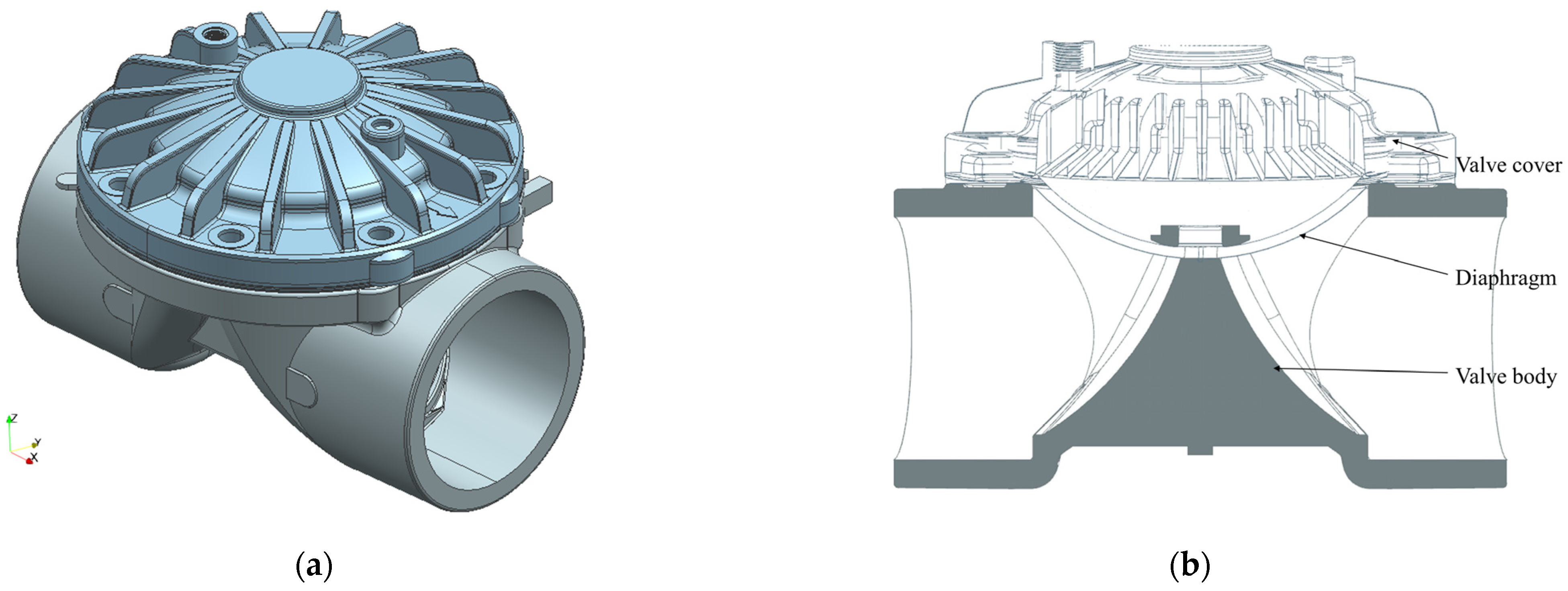
This study focuses on a diaphragm valve utilizing a rubber diaphragm as the sealing medium, with primary structural components including the valve cover, diaphragm, and valve body. The valve regulates fluid flow through the vertical displacement of the rubber diaphragm within the valve body, which opens or closes the flow channel. Constructed from cast iron, the valve features inlet and outlet inner diameters of 110.5 mm, with ordinary clean water serving as the working medium. Figure 1 illustrates the three-dimensional external geometry and internal longitudinal sectional structure of the valve, highlighting the spatial arrangement of its key components.

2.2. Mesh Generation

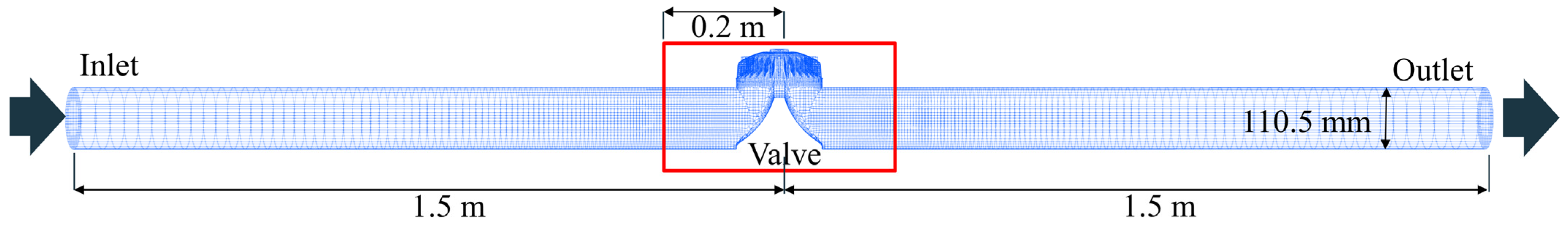
The internal flow domain of the diaphragm valve was meshed using the snappyHexMesh utility in OpenFOAM v8, which is well-suited for complex geometries. To capture flow dynamics accurately, local mesh refinement was applied within a 0.2 m range upstream and downstream of the valve body center, where flow velocity and pressure gradients are most intense. In compliance with the China’s national standard [20], the lengths of inlet and outlet straight-pipe extensions were set to at least 10 times the valve nominal diameter to ensure the fully developed flow conditions and to resolve the potential turbulent zones in the downstream. As depicted in Figure 2, the computational domain is defined with the valve body center as the origin, and the positive x-axis aligned with the flow direction (left to right in Figure 2), encompassing the valve and its extended upstream/downstream pipe segments.

2.3. Turbulence Models and Boundary Conditions

Governing equations were discretized using a second-order backward scheme for the temporal term, ensuring high accuracy in unsteady flow simulations. Spatial discretization of the convective and diffusive terms employed second-order upwind schemes to minimize numerical diffusion, while the pressure-velocity coupling was resolved using the PIMPLE algorithm for robust convergence. Therefore, the pimpleFoam solver, a semi-implicit pressure-based solver in OpenFOAM, was employed to handle the unsteady flow behavior and ensure numerical stability.

Reynolds-Averaged Navier–Stokes (RANS) methods were adopted for turbulence simulation, prioritizing computational efficiency while balancing accuracy. Five widely-used RANS-based turbulence models were evaluated: the Standard k-ε, Realizable k-ε, RNG k-ε, SST k-ω, and Spalart-Allmaras (S-A) models. These models differ in their treatment of turbulent viscosity, boundary layers, and rotational flows, providing a comprehensive basis for comparative analysis.

No-slip boundary conditions were applied to all solid wall boundaries, including the valve body and the internal surfaces of the inlet/outlet pipes (all made of cast-iron). The roughness of these internal surfaces can affect the simulated results, especially for the pressure drop. As stated in the hydraulic design manual [21], the roughness height (k_s) of cast-iron pipe material ranges from 0.2 to 0.5 mm, with an average value of 0.3 mm. Thus, a roughness height of 0.3 mm was used in the present simulation study, and the resulting pressure drop values confirmed the validity of the selected roughness height. The outlet boundary condition was set as zeroGradient for velocity. As to the inlet boundary conditions of velocity, two schemes were tested, which will be introduced in details in the Section 3.1.1.

For pipe flow, turbulence parameters, such as the turbulence kinetic energy k, dissipation rate ε, and related variables are determined by the following equations [4,9,22], where the volumetric flow rate Q and the valve pipe inner diameter d are known. The numerical methodology and parameter settings described herein provide a sound foundation for the subsequent simulation results.

$$U={\displaystyle \frac{4Q}{\pi d^2}}$$

(1)

$$\mathrm{Re}={\displaystyle \frac{\rho Ud}{\mu }}$$

(2)

$$l=0.038d_h$$

(3)

$$I=0.16{\mathrm{Re}}^{-0.125}$$

(4)

$$k={\displaystyle \frac{3{\left(IU\right)}^2}{2}}$$

(5)

$$\epsilon =C_{\mu }{\displaystyle \frac{k^{1.5}}{l}}$$

(6)

$${\nu }_t=C_{\mu }{\displaystyle \frac{k^2}{\epsilon }}$$

(7)

In the above equations, U denotes the mean flow velocity (m/s), d_h denotes the hydraulic diameter (m) which equals to d for circular pipe flow, l denotes the turbulence length scale (m), I denotes the turbulence intensity, and C_μ is a coefficient, taken as 0.09.

2.4. Mesh Independence Verification

To minimize discretization errors associated with mesh resolution and to ensure both mesh quality and accuracy, four cases with different mesh resolutions were tested, using the resulting head loss as the criterion for mesh independence. The goal was to achieve sufficient computational precision while reasonably reducing computing time.

Table 1. Head loss and mesh quality for various cases with different total number of mesh cells.

Mesh No.	Total Number of Mesh Cells	Head Loss (kPa)	Deviation from Mesh 1 (%)	y+ (-)	Average Non- Orthogonality (-)
1	148,154	11.89	-	125.9~215.3	10.20
2	451,083	12.00	0.93	88.6~148.6	8.39
3	716,554	11.63	−2.19	71.6~126.9	7.78
4	963,424	11.63	−2.19	65.6~112.1	7.35

summarizes the head losses for various total numbers of mesh cells at the same inlet flow rate of 62.550 m³/h. As the total cell number increases, the variation in head loss remains small: the deviation between Mesh 2 and Mesh 1 is 0.93%, the deviation between Mesh 3 and Mesh 1 is −2.19%, and the deviation between Mesh 4 and Mesh 1 is −2.19%. As to the mesh quality, y⁺ and non-orthogonality [22] are usually used to denote the quality of near-wall mesh and the angle of adjoint faces, respectively. The results shown in Table 1 indicates that both y⁺ and non-orthogonality decrease with the total mesh cells, which remains suitable for RANS modeling. Balancing computational cost and accuracy, Mesh 3 (716,554 elements) was selected for subsequent simulations, as it achieved stable results with acceptable numerical error.

2.5. Experimental Data

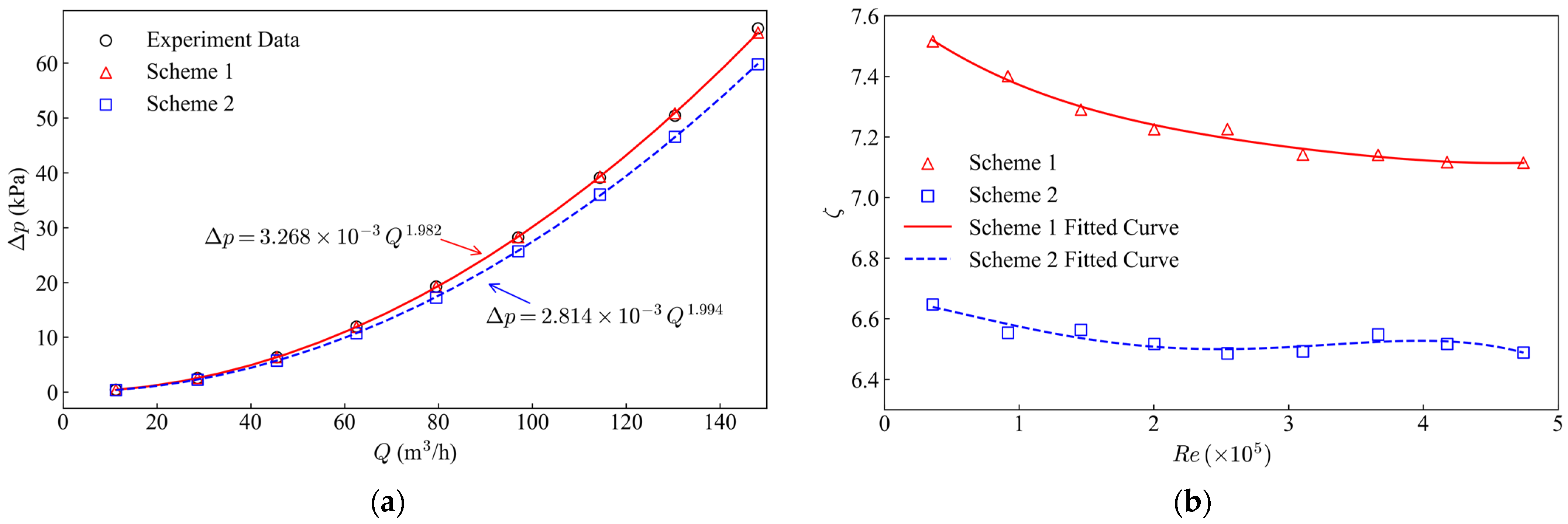
The validation of the present numerical modeling relies on experimental data provided by the valve manufacturer, as seen in Figure 3a, which was conducted by Fresno State International Center for Water Technology. This curve depicts the valve’s pressure-drop characteristics across a range of flow rates, with each data point representing the measured pressure drop at a specific flow rate. The experimental data served as a benchmark to validate the accuracy of simulation results under different inlet conditions and turbulence models.

2.6. Evaluation Metrics

Based on the China’s national standard [20], three important metrics are defined as following.

Head Loss Δp. It is defined as the net pressure drop across the valve, which should be calculated as the difference between the total pressure measured at points before and after the valve (including both the valve and upstream/downstream connecting pipes).

Flow Coefficient K_v. It is defined as the specific flow rate of water Q (m³/h) passing through the valve, at a specific Δp (kPa) of 100 kPa, within a temperature range of 5 to 40 °C. It can be calculated as

$$K_v=10Q\sqrt{{\displaystyle \frac{\rho }{{\rho }_0\Delta p}}}$$

(8)

where, ρ is the density of water (kg/m³), and ρ₀ is the density of water at 15 °C. Under ambient temperature conditions, the ratio ρ/ρ₀ is taken as 1, and this value is adopted in this study.

Flow Resistance Coefficient ζ. It is non-dimensional, closely related to the valve’s size, structure, and internal cavity shape. It can be calculated as

$$\zeta ={\displaystyle \frac{2000\mathrm{\Delta }p}{\rho v^2}}$$

(9)

where v denotes the average flow velocity in the pipe (m/s).

3. Results

3.1. Impact of Inlet Boundary Conditions on Head Loss

Two inlet schemes were evaluated to assess their influence on simulation accuracy at the valve’s maximum opening (64 mm, 100% opening). Scheme 1 (flowRateInletVelocity) and Scheme 2 (timeVaryingMappedFixedValue) were compared using the SST k-ω model, which demonstrated superior accuracy in preliminary tests.

3.1.1. Two Inlet Approaches

Scheme 1: flowRateInletVelocity. The inlet velocity U is initialized via the flowRateInletVelocity boundary condition by specifying the volumetricFlowRate. For each operating condition, a predefined volumetric flow rate is assigned.

Scheme 2: timeVaryingMappedFixedValue. Here, the initial values of U, k, ε, ω and ν_t at the inlet face are determined by interpolating a set of spatiotemporal point data. These data are stored in the boundaryData folder under the constant directory as boundary inlet conditions. Prior to the formal simulation, a 0.2 m inlet pipe segment is selected with cyclic boundary conditions applied at the inlet and outlet. Initial values for different operating conditions are calculated using Equations (1)~(7). After the flow in this development pipe reaches a fully developed state, data are extracted from the mid-section and then mapped as inlet profiles for the formal valve simulations.

3.1.2. Quantitative Comparison of Head Loss

As shown in Figure 3a, Scheme 1 predictions exhibited excellent agreement with manufacturer-provided experimental data, with a fitted power-law equation Δp = 3.268 × 10⁻³Q^1.982. In contrast, Scheme 2 results were systematically lower, described by Δp = 2.814 × 10⁻³Q^1.992. This discrepancy arises from Scheme 2’s reliance on interpolated profiles, which may underrepresent turbulent fluctuations near the valve inlet in the experimental flow condition. As shown in Figure 3b, the flow resistance coefficient ζ decreased nonlinearly with the Reynolds number (Re), reflecting reduced flow obstruction at higher velocities. For Re ranging from 0.4 × 10⁵ to 4.8 × 10⁵, ζ dropped from 7.51 to 7.11 in Scheme 1 and 6.65 to 6.49 in Scheme 2, indicating consistent trends but subtle differences in turbulence intensity representation between the two inlet schemes.

3.1.3. Flow Coefficient Validation

Table 2. Flow coefficients for different inlet condition.

	1	2	3	4	5	6	7	8	9
Q/(m3/h)	11.265	28.663	45.584	62.550	79.540	97.028	114.448	130.438	148.131
Scheme 1 (Kv)	178.012	179.385	180.742	181.552	181.545	182.611	182.622	182.931	182.952
Scheme 2 (Kv)	189.285	190.626	190.489	191.165	191.623	191.520	190.705	191.160	191.582

lists the flow coefficient K_v, a key metric for valve capacity, under different inlet conditions. Scheme 1 yielded K_v values between 178.0 and 182.9, with minimal variation at high flow rates, confirming stable flow capacity of the valve. Scheme 2 showed slightly higher K_v (between 189.3 and 191.6), aligning with its lower head loss predictions. These results highlight the critical role of inlet boundary conditions in capturing realistic flow dynamics, with direct volumetric flow input providing more reliable validation against experimental data.

3.2. Comparative Analysis of Turbulence Models

Five RANS-based turbulence models were evaluated to identify the most accurate solver for diaphragm valve simulations, focusing on head loss predictions and flow field details.

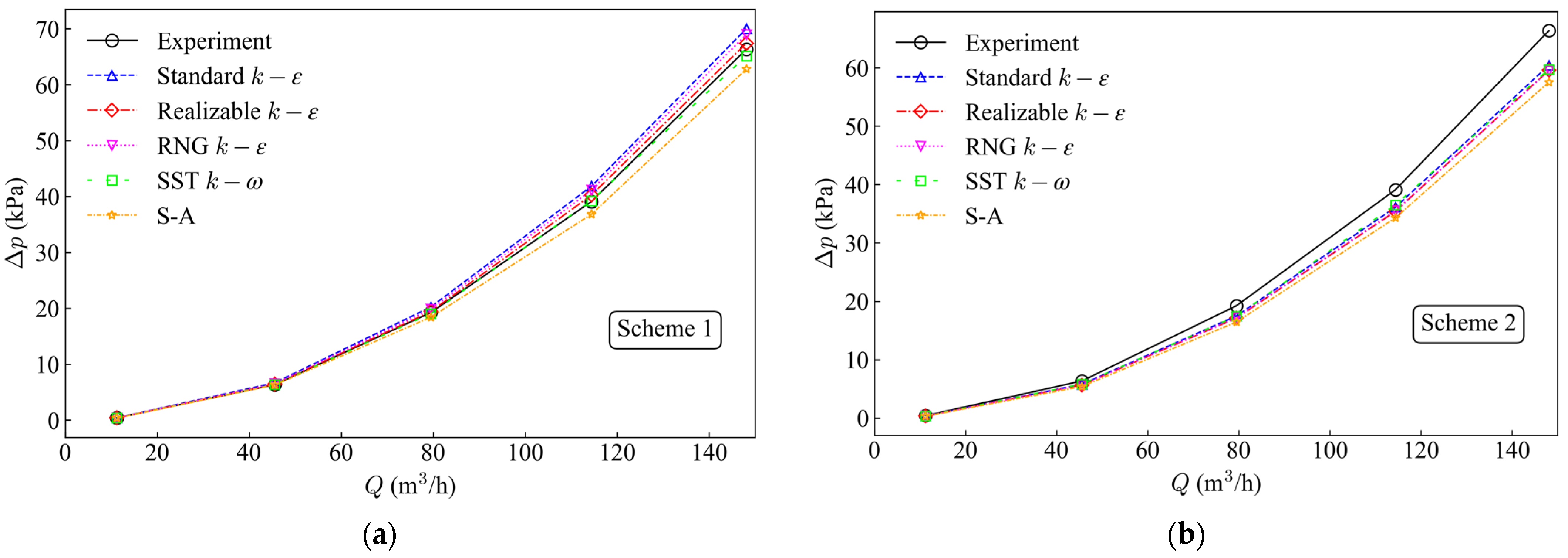
3.2.1. Head Loss Accuracy

Figure 4 presents the simulated head loss (Δp) at varying flow rates for both inlet schemes, with experimental measurement compared against results from the five RANS-based turbulence models. The results indicate that, compared to experimental data, the standard k-ε model and the Spalart-Allmaras (S-A) model exhibit the lowest computational accuracy in Scheme 1, as shown in Figure 4a. Conversely, the SST k-ω model demonstrates the highest accuracy, featuring a minimum deviation of 0.29% and a maximum deviation of 2.43%. For Scheme 2, as shown in Figure 4b, predictions from all five turbulence models systematically underestimate the experimental head loss values. Among these, the S-A model shows the poorest performance, with deviations exceeding 12% across all flow conditions and a peak deviation of 18.42%. The remaining four models exhibit relatively minor discrepancies in their predictions, with the standard k-ε model and the SST k-ω model models demonstrating comparatively better computational accuracy.

In order to quantify the data in Figure 4, regression analysis was conducted for both the experimental measurements and the numerical predictions from each turbulence model, as shown in

Table 3. Coefficients of the regression analysis for both the experimental measurements and the numerical predictions from each turbulence model.

Coefficients	Experiment	Standard k-ε	Realizable k-ε	RNG k-ε	SST k-ω	S-A
m1 (×10−3)	2.922	3.264	3.092	3.099	3.405	2.961
n1	2.006	1.995	1.999	2.003	1.973	1.992
R12	0.99993	1.00000	1.00000	1.00000	1.00000	0.99977
m2 (×10−3)	2.922	2.846	2.648	2.767	3.347	2.506
n2	2.006	1.993	2.005	1.996	1.959	2.009
R22	0.99993	1.00000	0.99999	1.00000	0.99987	1.00000

. The fitted function for each condition follows

$$\mathrm{\Delta }p=m{Q}^n$$

(10)

where m and n are coefficients to be fitted. The fitted coefficients, along with the regression coefficient (R²), for different schemes and different turbulence models can be found in Table 3. Although the fitted coefficients (m, n) vary across different inlet schemes and turbulence models, the exponential relationship holds consistent across various volumetric flow conditions despite differing fitting coefficients. The subscripts 1 and 2 represent inlet condition Scheme 1 and Scheme 2, respectively. Combining the numerical simulation results of both schemes, the accuracy of different turbulence models is generally consistent for the low flow rates. However, as the flow rate increases, the simulated values deviate more significantly from the experimental values, with a maximum deviation of 6.97% in Scheme 1 and 13.30% in Scheme 2. Across both schemes, the SST k-ω turbulence model consistently demonstrates the highest computational accuracy, suggesting that the SST k-ω model is currently one of the more accurate turbulence models in the field of hydraulic numerical simulation for calculating the hydraulic performance of valves.

3.2.2. Flow Field Visualization

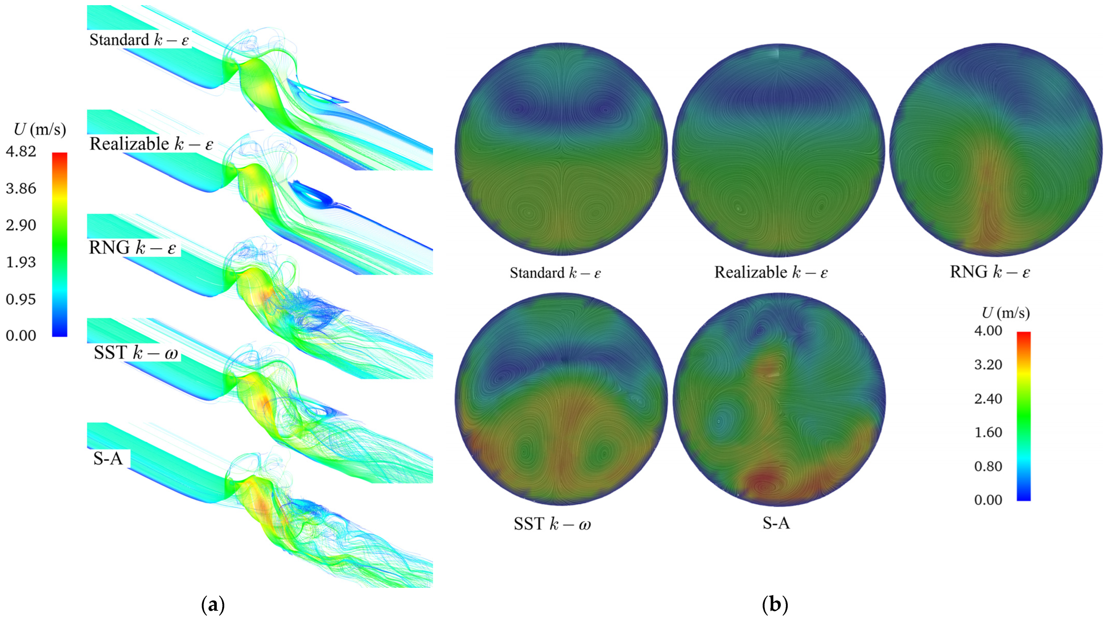
This study selected an inlet flow rate of 45.584 m³/h as the flow condition to compare the different turbulence models. As shown in the streamline comparison in Figure 5a, all five turbulence models exhibit smooth streamlines and stable flow patterns within the inlet pipe. In the valve and post-valve regions, the standard k-ε model produces the smoothest flow field streamlines, with no significant vortices or fluctuations as the fluid passes through the valve, and relatively lower peak velocities. The Realizable k-ε model captures more flow details compared to the standard k-ε model, with vortices appearing in the upper post-valve region. The other three turbulence models provide even richer flow details of simulation, revealing a greater number of vortices.

This phenomenon can be attributed to the fact that the standard k-ε model, being a high-Reynolds-number model, performs poorly in simulating rotational flows and boundary layer separation, often leading to distorted results, which explains the smoother appearance of its flow field streamlines. In contrast, the Realizable k-ε model and the RNG k-ε model account for the effects of turbulent vortices and incorporate improvements in turbulent viscosity, enabling better handling of high-curvature and rotational flows, thus enhancing simulation accuracy. The SST k-ω model combines the strengths of the k-ε and k-ω models, making it well-suited for complex flow simulations. Lastly, the S-A model, which requires solving only a single transport equation, offers relatively faster computation speeds and performs well in simulating adverse pressure gradient conditions.

Figure 5b illustrates the velocity contour and streamline diagrams at the valve outlet cross-section in the x-direction of flow for various turbulence models. The high-velocity region is predominantly located in the lower part of the circular flow channel, while the middle and upper regions exhibit lower velocities, even forming stagnant zones. Within the flow field, the streamlines of the standard k-ε model and the Realizable k-ε model display a left-right symmetrical distribution, both generating vortices. However, the former produces vortices in both the upper and lower regions, whereas the latter generates vortices only in the lower part of the pipe. Similarly, the RNG k-ε model produces vortices solely in the lower region. The S-A model exhibits the most intense vortices in its flow field simulation, with the most significant variation in velocity distribution and slightly higher velocity values compared to the other turbulence models. In contrast, the vortex and streamline distribution in the SST k-ω model is less intense than that of the S-A model, with the vortices in the lower region displaying a left-right symmetrical pattern.

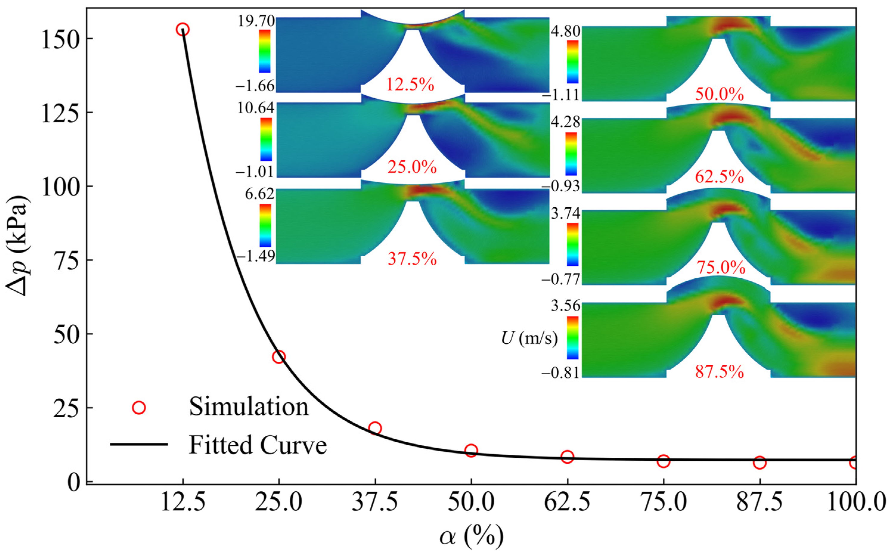
3.3. Head Loss Variation with Valve Opening

The variation in head loss under steady-state conditions for different diaphragm valve openings was analyzed across various flow regimes. Diaphragm valves achieve opening and closing through the deformation of the diaphragm, and the degree of opening can be adjusted by altering the distance between the bottom of the diaphragm and the valve weir. In this study, the diaphragm valve model was established with openings of 8, 16, 24, 32, 40, 48, 56, and 64 mm, where 64 mm represents the position of full opening. These openings (α) are sequentially defined as 12.5%, 25%, 37.5%, 50%, 62.5%, 75%, 87.5%, and 100% of the diaphragm valve opening, respectively, with the opening denoted by α. Figure 6 illustrates the head loss under stable conditions at different diaphragm openings for an inlet flow rate of 45.584 m³/h, with the regression equation provided as Δp = 588.377Q^−11.176α + 7.219, R² ≈ 0.99957.

Table 4. Head losses (unit in kPa) at different flow rate and different valve openings, with corresponding regression equations.

Flow Rate (m3/h)	α (%)
	12.5	25.0	37.5	50.0	62.5	75.0	87.5	100.0
11.265	9.38	2.62	1.11	0.67	0.50	0.44	0.40090	0.40049
	Δp = 35.647Q−11.085α + 0.452, R2 ≈ 0.99962
45.584	153.01	42.15	17.95	10.39	8.28	6.79	6.42	6.36
	Δp = 588.877Q−11.176α + 7.219, R2 ≈ 0.99957
114.448	962.55	265.46	112.70	64.73	49.98	42.20	39.64	39.27
	Δp = 3691.904Q−11.141α + 44.541, R2 ≈ 0.99959

presents the head loss under different flow rates and valve openings. The simulation results indicate that the trend of head loss variation with valve opening remains consistent across different flow conditions. Specifically, when the valve opening increases from 0% to 50%, the head loss changes dramatically. Furthermore, an exponential relationship exists between the head loss of the diaphragm valve and its opening, and this relationship holds consistent across various flow conditions.

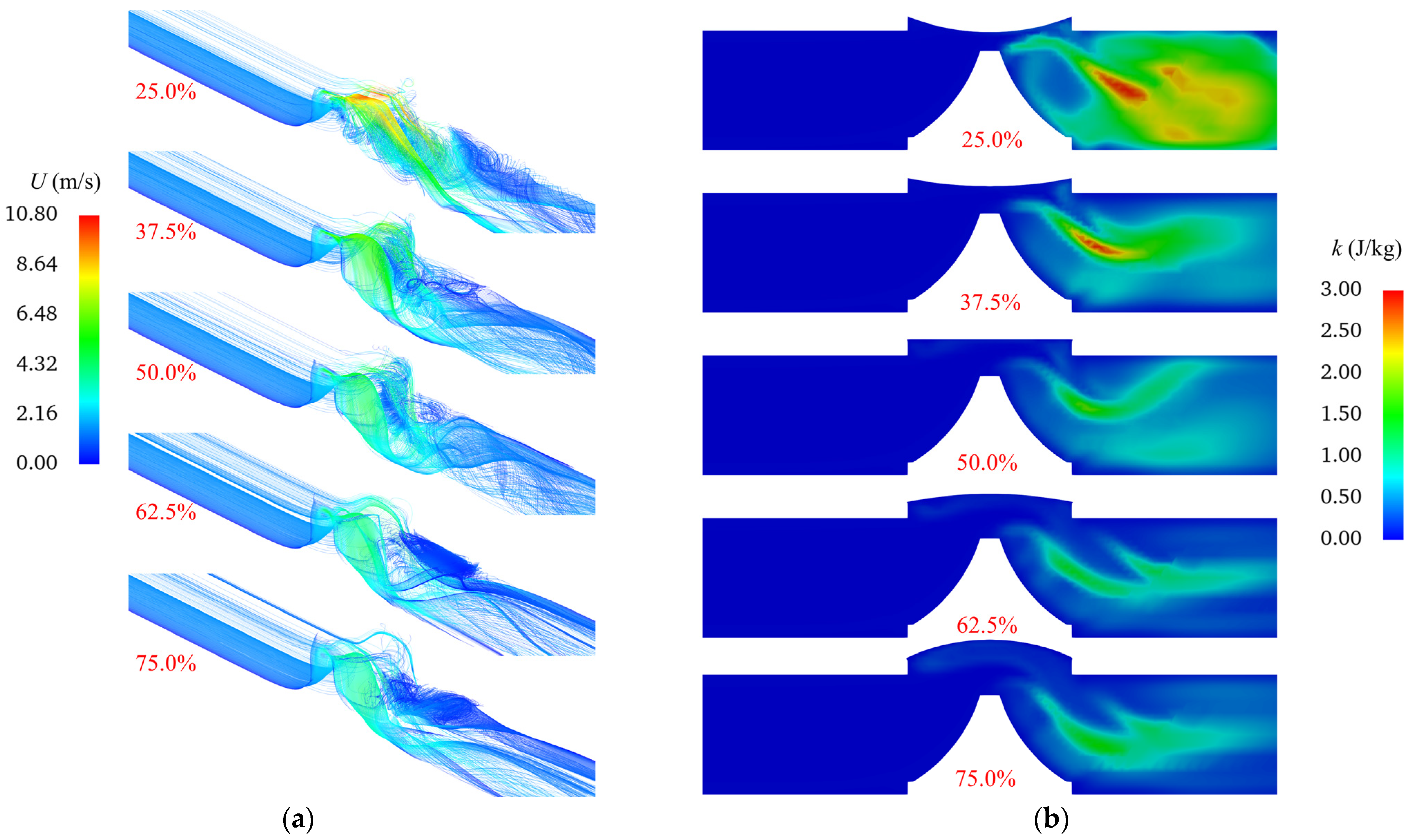
The flow characteristics of the diaphragm valve were investigated under a flow condition of 45.584 m³/h by analyzing the steady-state flow field distribution at different valve openings. The velocity streamlines and turbulent kinetic energy at various openings are depicted in Figure 7a,b. At all valve openings, the flow in the upstream inlet pipe section remains steady, characterized by uniformly distributed velocity streamlines of similar magnitude and no significant signs of turbulence.

At small valve openings, the flow field within the valve exhibits intense fluctuations, generating strong turbulent kinetic energy in the downstream region. Notably, most of this turbulent energy is not dissipated locally but is advected downstream. In contrast, at larger openings, streamline curvature within the valve decreases, leading to smoother flow transitions and the formation of a stagnant flow zone in the upstream portion of the downstream region. As the valve opening increases, turbulent energy progressively diminishes due to reduced flow separation and shear forces.

4. Conclusions

This study numerically investigates the hydraulic performance of a diaphragm valve, focusing on inlet boundary conditions, turbulence model accuracy, and head loss characteristics across different openings. Key findings are as follows:

Inlet Boundary Condition Impact. Two inlet schemes were tested at the maximum valve opening. Scheme 1 (flowRateInletVelocity) showed excellent agreement with experimental data, accurately capturing turbulent dynamics. In contrast, Scheme 2 (timeVaryingMappedFixedValue) underestimated head loss due to insufficient representation of inlet turbulent fluctuations. Scheme 1 is thus more reliable for realistic simulation and validation.

Turbulence Model Performance. Among five evaluated models, the SST k-ω model demonstrated the highest accuracy in predicting flow fields and head loss, effectively resolving complex features like vortices and boundary layer interactions, especially under adverse pressure gradients. The Spalart-Allmaras model performed poorly, lacking detail in intricate flow structures. Other k-ε variants (Standard, Realizable, RNG) offered moderate accuracy, with Realizable and RNG slightly improving rotational flow representation over the Standard k-ε model.

Head Loss vs. Valve Opening. Under varying flow rates, head loss exhibited a consistent exponential decrease with increasing valve opening. The most significant changes occurred below 50% opening, coinciding with high post-valve turbulent energy. At larger openings, flow stabilized, turbulent energy reduced, and stagnant zones formed. This exponential relationship holds across different flow rates, providing a robust basis for predicting hydraulic behavior.

Practical Insights. The study highlights the importance of selecting direct volumetric flow boundaries and the SST k-ω model for reliable CFD simulations. The established exponential correlation between head loss and opening offers engineering guidance for optimizing diaphragm valve design and system efficiency in irrigation and water distribution networks.

Despite the above key findings, there are also some limitations in this study: near-wall meshing used high y⁺ values, potentially affecting boundary layer accuracy; only steady-state RANS models were tested, neglecting unsteady flows and advanced turbulence approaches; experimental validation lacked detailed flow field data; diaphragm flexibility and fluid-structure interaction were not modeled; inlet conditions assumed fully developed flow, ignoring upstream disturbances.

Future research should refine near-wall resolution with low-Reynolds models, incorporate fluid-structure interaction to account for diaphragm deformation, explore unsteady DES/LES simulations, validate against detailed experimental measurements (e.g., PIV), and investigate upstream flow disturbances to improve simulation realism and predictive capability.

References

- Cană, P.; Ripeanu, R.G.; Diniță, A.; Tănase, M.; Portoacă, A.I.; Pătîrnac, I. A review of safety valves: Standards, design, and technological advances in industry. Processes 2025, 13, 105. [Google Scholar] [CrossRef]
- Jerman, H. Electrically activated normally closed diaphragm valves. J. Micromech. Microeng. 1994, 4, 210. [Google Scholar] [CrossRef]
- Hannig, M.; Höhne, F.; Langbein, S. Valve Technology: State of the Art and System Design. In Shape Memory Alloy Valves; Czechowicz, A., Langbein, S., Eds.; Springer International Publishing AG: Cham, Switzerland, 2015; pp. 3–22. [Google Scholar]
- Liu, J.; Yu, Y. The construction of the numerical model of the internal flow field and an analysis of the flow characteristics of the diaphragm solenoid valve. China Rural. Water Hydropower 2024, 2, 121–128. (In Chinese) [Google Scholar] [CrossRef]
- Koech, R.; Smith, R.; Gillies, M. Automation and control in surface irrigation systems: Current status and expected future trends. In Proceedings of the 2010 Southern Region Engineering Conference (SREC 2010), Toowoomba, Australia, 11–12 November 2010. [Google Scholar]
- Wen, F.F.; Cheng, Y.G.; Meng, W.W. Dynamic hydraulic characteristics of a prototype ball valve during closing process analysed by 3D CFD method. IOP Conf. Ser. Earth Environ. Sci. 2018, 163, 12115. [Google Scholar] [CrossRef]
- Habibnejad, D.; Akbarzadeh, P.; Salavatipour, A.; Gheshmipour, V. Cavitation reduction in the globe valve using oblique perforated cages: A numerical investigation. Flow. Meas. Instrum. 2022, 83, 102110. [Google Scholar] [CrossRef]
- Ge, P.; Ma, S.; Zhang, J.; Li, Y.; Ren, L. Transient flow characteristics analysis of PVC ball value based on dynamic mesh. J. Water Resour. Archit. Eng. 2022, 20, 130–135. [Google Scholar] [CrossRef]
- Munsch, P.; Kiermeir, J.; Schilling, R.; Schlücker, E.; Skoda, R. Three-dimensional simulation of cavitating flow in reciprocating positive displacement pumps with fluid-actuated valves. J. Fluid. Eng. 2025, 147, 041201. [Google Scholar] [CrossRef]
- Chen, P.; Liu, Z.; Xu, R.; Liu, J. Comparative investigation and test verification of cavitation and turbulence models of injector control ball valve. Int. J. Heat Fluid Flow 2024, 109, 109557. [Google Scholar] [CrossRef]
- Zhao, M.; Wei, T.; Hao, S.; Ding, Q.; Liu, W.; Li, X.; Liu, Z. Turbulence simulations with an improved interior penalty discontinuous Galerkin method and SST k-ω model. Comput. Fluids 2023, 263, 105967. [Google Scholar] [CrossRef]
- Bai, L.; Hu, C.; Wang, Y.; Han, Y.; Agarwal, R.; Zhou, L. Evaluation of various turbulence models and large eddy simulation for stall prediction in a centrifugal pump. Water 2023, 15, 3432. [Google Scholar] [CrossRef]
- Brazhenko, V.; Cai, J.; Fang, Y. Utilizing a transparent model of a semi-direct acting water solenoid valve to visualize diaphragm displacement and apply resulting data for CFD analysis. Water 2024, 16, 3385. [Google Scholar] [CrossRef]
- Bellegoni, M.; Cotteleer, L.; Raghunathan Srikumar, S.K.; Mosca, G.; Gambale, A.; Tognotti, L.; Galletti, C.; Parente, A. An extended SST k−ω framework for the RANS simulation of the neutral Atmospheric Boundary Layer. Environ. Model. Softw. 2023, 160, 105583. [Google Scholar] [CrossRef]
- Gimenez, J.M.; Bre, F. An enhanced k-ω SST model to predict airflows around isolated and urban buildings. Build. Environ. 2023, 237, 110321. [Google Scholar] [CrossRef]
- Yan, X.; Wang, X. Improving modeling of submerged canopy flows with a vortex-based Spalart–Allmaras model. J. Hydrol. 2024, 635, 131174. [Google Scholar] [CrossRef]
- Alauzet, F.; Spalart, P. A new rotation correction for the Spalart-Allmaras model to improve off-body vortex prediction and vortex-vortex interaction effect. In Proceedings of the AIAA SCITECH 2024 Forum, Orlando, FL, USA, 8–12 January 2024. [Google Scholar]
- Gao, F.; Wang, H.; Wang, H. Comparison of different turbulence models in simulating unsteady flow. Procedia Eng. 2017, 205, 3970–3977. [Google Scholar] [CrossRef]
- Zhang, Y.; Zhang, D.; Jiang, H. Review of challenges and opportunities in turbulence modeling: A comparative analysis of data-driven machine learning approaches. J. Mar. Sci. Eng. 2023, 11, 1440. [Google Scholar] [CrossRef]
- GB/T 30832-2014; Valves–Test Method of Flow Coefficient and Flow Resistance Coefficient. Standards Press of China: Beijing, China, 2014. Available online: https://openstd.samr.gov.cn/bzgk/gb/newGbInfo?hcno=9D5005ECB4AFE1D35E787CB2AFE428D0&refer=outter (accessed on 8 May 2025). (In Chinese)
- Liu, Z.; Wang, D.; Wang, D. Handbook of Hydraulic Structure Design, 2nd ed.; China Water Resources and Hydropower Publishing House: Beijing, China, 2011; Volume 1. [Google Scholar]
- Xu, Y.; Liu, X. An immersed boundary method with y+-adaptive wall function for smooth wall shear. Int. J. Numer. Methods Fluids 2021, 93, 1929–1946. [Google Scholar] [CrossRef]