Impact of Filtration Cycle Patterns on Both Water and Energy Footprints in Drip Irrigation Systems

Abstract

Drip irrigation is a widely spreading technology, mainly due to its high water-use efficiency. This technique requires a filtration process that exhibits cyclical behavior where both filtration and backwashing modes repeat. In filtration, pressure increases with time due to the particle retention up to a preset value. In backwashing, the flow is reversed to clean the filter. Different design strategies to reduce energy and water consumption have been proposed, but their practical effects are not yet clear. Here, a global analysis method based on the classification of the time evolution of the pressure curve in filtration mode was developed. Energy and water use efficiency indices were defined and evaluated under different scenarios. More design options can be undertaken to reduce the consumption of energy than of water. The decrease in the pressure drop for clean filter conditions arose as the best option to increase energy efficiency (in a realistic scenario, a reduction of 20% in the pressure drop with tap water resulted in a reduction of 7.6% in the energy consumption per volume of filtered water). Precise backwashing times and flow rates were essential to improve water use efficiency (e.g., doubling the backwashing time led to a 4.5% decrease in water use efficiency).

1. Introduction

International organizations [1] as well as national [2] and supranational [3] policies promote the efficient use of water. The reuse of treated water is particularly encouraged, although the cost may limit its spread [4]. In agriculture, drip irrigation offers superior water use efficiency in comparison with traditional irrigation methods, and it mitigates hazards regarding wastewater reuse [5]. This technology appears suitable for regions sensitive to suffering water scarcity or severe droughts. In Spain, for example, drip irrigation feeds 58% of the irrigated agricultural area [6], and consumes only 40% of all the irrigation water [7]. India, China, USA and other countries are also expanding drip irrigation use [8].

Emitter clogging is a major threat to drip irrigation [9] where sediment concentration of the influent and irrigation time are important factors for determining the reliability of the system [10]. The application of phosphorus fertilizer and water with high Ca²⁺ concentrations also compromise the emitter clogging [11]. Therefore, water must be filtered prior to its downstream release to mains, laterals and drippers. The filtration process can be carried out with several retention mechanisms such as porous media beds [12], packed discs [13], and screens [14]. Filters behave cyclically with two different working modes: filtration and backwashing. In filtration mode, the filter begins to work close to pristine conditions, this being reflected in a small pressure drop across the filter body. This pressure drop steadily increases as the filter element captures particles of the influent, ultimately reaching a predefined threshold value where filtration stops [15]. At this point, the backwashing mode begins, where non contaminated water flows upstream to detach particles from the filter element and to drag them out of the system [16]. Thus, the filter recovers its initial condition to initiate another cycle. This whole process is often automated by means of differential pressure sensors, three-way valves, and the required setup [17].

Pressurized filters demand energy to drive pumps, which can be a substantial drawback when compared to other irrigation methods [18]. In addition, the backwashing mode wastes water when it is not reincorporated upstream. As a result, the efficient use of energy and water in drip irrigation emerges as a clear concern that must be addressed [19].

Filtration is a ubiquitous process in many sectors, and researchers have focused on determining the operational conditions that provide the optimum filtration cycle. These conditions highly depend on the filtration procedure (i.e., constant pressure, constant flow rate, etc.), filter type, and water quality [20]. In self-cleaning screen filters, the influence of the backwashing time on the hydraulic performance is very relevant [21], since the retention capacity of the filter must be fully recovered. The porosity level of the filter cake growth on the screen arises as a relevant parameter for determining the cleaning time [22]. Recently, screen cleaning by a jet has been proved to be a very efficient method in terms of water savings [23]. In disc filters, changes in the geometry of the engraved channels in the individual discs may remarkably reduce the pressure drop without penalizing the collection of particles [24], or even slightly improve the whole filtration capacity [13]. In porous media filters, analyses of different materials with controlled levels of contaminant particles have revealed that glass beads are not suitable for micro irrigation, and more irregular shaped materials such as quartz sand are recommended [25].

The previous studies were case-dependent, since improvements were proposed for a particular filter design working with specific operational conditions and influent qualities. However, there is not a clear general design rule and/or a recommendation guide about how to proceed for upgrading water and energy use efficiencies of pressurized filters for drip irrigation. Two main global design strategies have been detected: one in which filter modifications aim to reduce the pressure drop under tap water conditions [26,27], and another in which the purpose is to increase the duration of the filtration mode [14,28,29]. However, as before, these strategies have been targeted at specific filter designs, and all lack quantitative analyses of water plus energy saving effects.

Here, a global approach was applied, not focusing on a particular filter but on the general form of the filtration curve (pressure drop variation versus time). The goal was to quantify the impact of modifying the filtration cycle patterns on the reduction in water and/or energy consumption in drip irrigation systems, thereby providing manufacturers with quantifiable directions for filter design improvements. Analyses of field and laboratory data of different filtration technologies applied to drip irrigation [13,21,22,23,24,25,30,31,32,33,34,35,36,37,38] suggested that the trend of the filtration cycle may be classified into three main categories (Figure 1). This classification was later confirmed by own in-field experiments with a porous media filter. As expected, the filtration mode dominates, in time, over the backwashing one in all scenarios.

The time evolution of the filter pressure drop in filtration mode was close to linear (Figure 1A) for the following: different disc and screen filters working with a fish farm effluent [33]; porous media filters fed with the outlet of the tertiary of a municipal waste water treatment plant (WWTP) (present study from unpublished data of [32]) and with sandy water filtered with different types of porous media [25,36]; disc filters using water with different concentration of algae and organic particles [30]; varying concentrations of compound fertilizers [35]; and in laboratory conditions with controlled particle gradations [24]. Other authors have reported filtration cycles that resemble piecewise linear functions (Figure 1B) of the filter pressure drop as a function of time. This type of behavior is characterized by an initial period with an almost unnoticeable increase in the filter pressure variation, being recently reported in state-of-the-art screen filters in laboratory analyses with water contaminated with particles whose size gradation and concentration levels mimicked those found in sediments of actual irrigation water [21,22,23], with particles originated from biogas slurry [37], and using commercial self-cleaning screen filters for drip irrigation with two qualities of sand–water mixtures [34]. The piecewise linear trend was also observed when using porous media filters with inorganic particles in laboratory analyses [38], as well as in novel disc filters analyzed under different influent sediment types and concentrations [13,31,37]. The quadratic behavior of the pressure drop as a function of time (Figure 1C) was clearly observed in disc filters for drip irrigation when dispersing diatomite under laboratory conditions [31], and also in self-cleaning screen filters with a fine mesh working with low sediment concentrations [34]. Both piecewise linear and quadratic type curves for the filtration modes were also identified for different runs in porous media filters using water from the tertiary of a municipal WWTP (present study from unpublished data of [32]).

The trends shown in Figure 1, and analyzed in the present study, specifically avoided filter stages near to clog, in which the pressure drop across the filter finally stabilizes up to a maximum value, describing characteristic S-type curves, as has been reported in screen [22,35] and disc filters [13,24]. The reason was that the recommended operational conditions for real applications should define a setpoint value for initiating the backwashing process well before the occurrence of such a final stage [14].

Of course, the trend of the filter pressure drop as a function of time is highly dependent on operational conditions (mainly flow rate), water quality (characteristics and quantity of particles), and filter design. The global approach here carried out intended to provide discussions valid for any technology and with any flow rate by defining two normalized indices that provide insight into both energy and water use efficiency. The first index is the amount of energy consumed per cycle divided by the amount of filtered water (i.e., usable water for drip irrigation). The second index corresponds to the ratio between filtered water and total (filtered plus backwashed) water used per cycle.

Changes in the quality of irrigation water and/or filter design may lead to substantial modifications in the filtration cycle. Those related to filter design are more controllable, being likely to be fundamental in the decision-making process of novel designs. Therefore, the consequences of modifying the main parameters that define the patterns of the filtration cycles shown in Figure 1 on the values reached by the two indices were explored. As an example for the filtration mode of the linear trend (Figure 1A), new filter designs that reduce the pressure drop under tap water conditions (or, equivalently, under clean filter conditions) (M1 in Figure 2A) in comparison with the nominal case (N in Figure 2A) decrease the energy use per unit time, as this value is proportional to the area under the pressure drop curve. However, this strategy does not alter water use, since the same number of full cycles is needed. A different design only focused on prolonging the filtration cycle (M2 in Figure 2B) in comparison with the nominal case maintains the same energy use per unit time but increases the water use efficiency as it reduces the number of backwashing periods. Filter designs that combine both reduction in initial pressure drop and extension in the duration of the filtration mode provide benefits in both energy and water use (Figure 2C).

As can seen above, the purpose of the present work was to quantify the effects of modifying the global coefficients that describe the time evolution of the filter pressure drop on both energy and water efficiency indices. In Section 2, literature data as well as the experimental setup and the corresponding results that support the behavior displayed in Figure 1 are exposed. Also in this section, the global equations that describe three types of filter pressure drop evolutions as a function of time, and their efficiency indices, are developed. Results obtained by varying the main coefficients that modulate the temporal evolution of these three types of filter pressure drop curves are presented in Section 3. The discussion of applying alternative conditions (pump curves, setpoints, etc.) and their comparison with the previous results is conducted in Section 4. Finally, the main conclusions are listed in Section 5.

2. Materials and Methods

2.1. Experimental Setup

The experimental setup is described in detail in [38], where the solid removal efficiencies in a porous media laboratory (i.e., scale) filter were analyzed at different media depths, with different clogging particles, and with different filtration and backwashing superficial velocities. The studies conducted in [32] focused on the conditions of the filter (mass retained) at the end of the filtration process, avoiding analyses about its transient behavior. Here, this transitory trend was examined to support the identification of general filtration cycle patterns, as pointed out previously.

The experiments used a laboratory porous medium filter of 110 mm inner diameter made of polymethyl methacrylate with the underdrain consisting of a stainless steel perforated plate above which 200 mm of commercial calibrated silica medium CA07MS (Sibelco Hispania, Bilbao, Spain) was added after being washed and dried. The characteristics of this silica sand in terms of D₁₀ and D₆₀ diameters (diameter below which the finer sample accounted for 10% and 60% in weight) were 0.48 mm and 0.83 mm, respectively, whereas the ratio of voids to total volume (porosity) was 0.40. These technical specifications agreed with the G1 grain size distribution in [39] (D₁₀ = 0.50 mm, D₆₀ = 0.76 mm, and porosity equal to 0.43), who examined the effect of using different media bed characteristics in three commercial media filters for drip irrigation. This porous medium, subsequently sieved to reduce the D₆₀ − D₁₀ range, has also been extensively used in comparative studies with tap water, such as a recent one dealing with different underdrain designs [40]. Other materials were not investigated, since silica sand is the most common choice for irrigation media filters and evinces a remarkable filtration capacity in comparison with some other products [25].

The filter pressure drop was measured with a digital manometer (Leo2, Keller, Winterthur, Switzerland; ±0.07% accuracy) connected at both inlet and outlet filter pipes that were selected through a switch valve. Inlet water was pumped from a filtered effluent of the outlet chamber of the settling tanks of the WWTP in the city of Celrà (Girona, Spain). The system included a centrifugal pump (Niza 60/3, Hidráulica Alsina, La Llagosta, Spain), a flow meter (CZ30000 DN15, Contazara, Zaragoza, Spain; ±1% accuracy), and gate valves to regulate the flow rate, with all of the system working in open circuit mode. Data about filtered volume, flow rate, pressures at filter inlet and outlet, and temperature were recorded every 150 s, which was sufficient to capture the trend of the pressure drop versus time curve since experiments ranged from 3450 to 20,100 s. The experiments ended when the filter pressure drop (inlet minus outlet pressure values) rose 50 × 10³ Pa above the initial, clean filter conditions value. Four repetitions with superficial velocities equal to 30 m h⁻¹ and 60 m h⁻¹ were carried out.

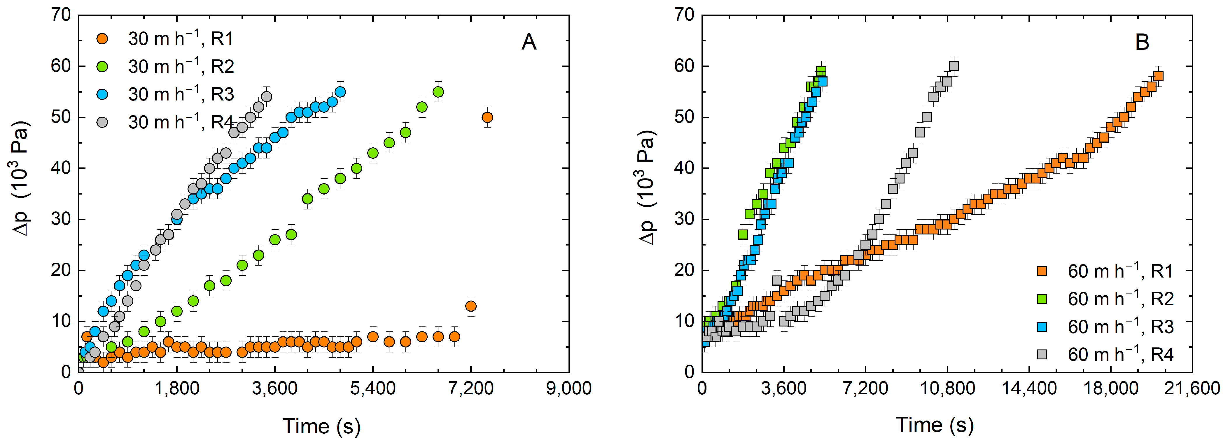
2.2. Experimental Results

The filter pressure drop data Δp as a function of time revealed different behaviors (Figure 3). With a superficial velocity of 30 m h⁻¹ (Figure 3A), repetitions 3–4 almost replicated the same temporal evolution, clearly showing a linear response. The physical properties of the reclaimed effluent substantially varied along repetition 1, with a sudden increase in turbidity of the reclaimed effluent at the end of the filtration regime, leading to an abrupt piecewise linear behavior. Similar rapid increases in the filter pressure drop after a long period with almost no changes have been reported without modifying the characteristics of the influent (e.g., [23]). With a superficial velocity of 60 m h⁻¹ (Figure 3B), repetitions 2 and 3 behaved similarly, but lower turbidity levels of the reclaimed effluent were registered in repetitions 1 and 4. In this case, repetition 1 exhibited a linear evolution, although with a milder slope than in R2–R3, whereas repetition 4 evolved with a pattern that could be classified into the quadratic category. The experimental data confirmed that the time evolution of the pressure drop for a given filter depends on the quality of the influent. This emphasizes the importance of knowing the water quality to choose the correct filter design. This fact, on the other hand, does not invalidate the results obtained here.

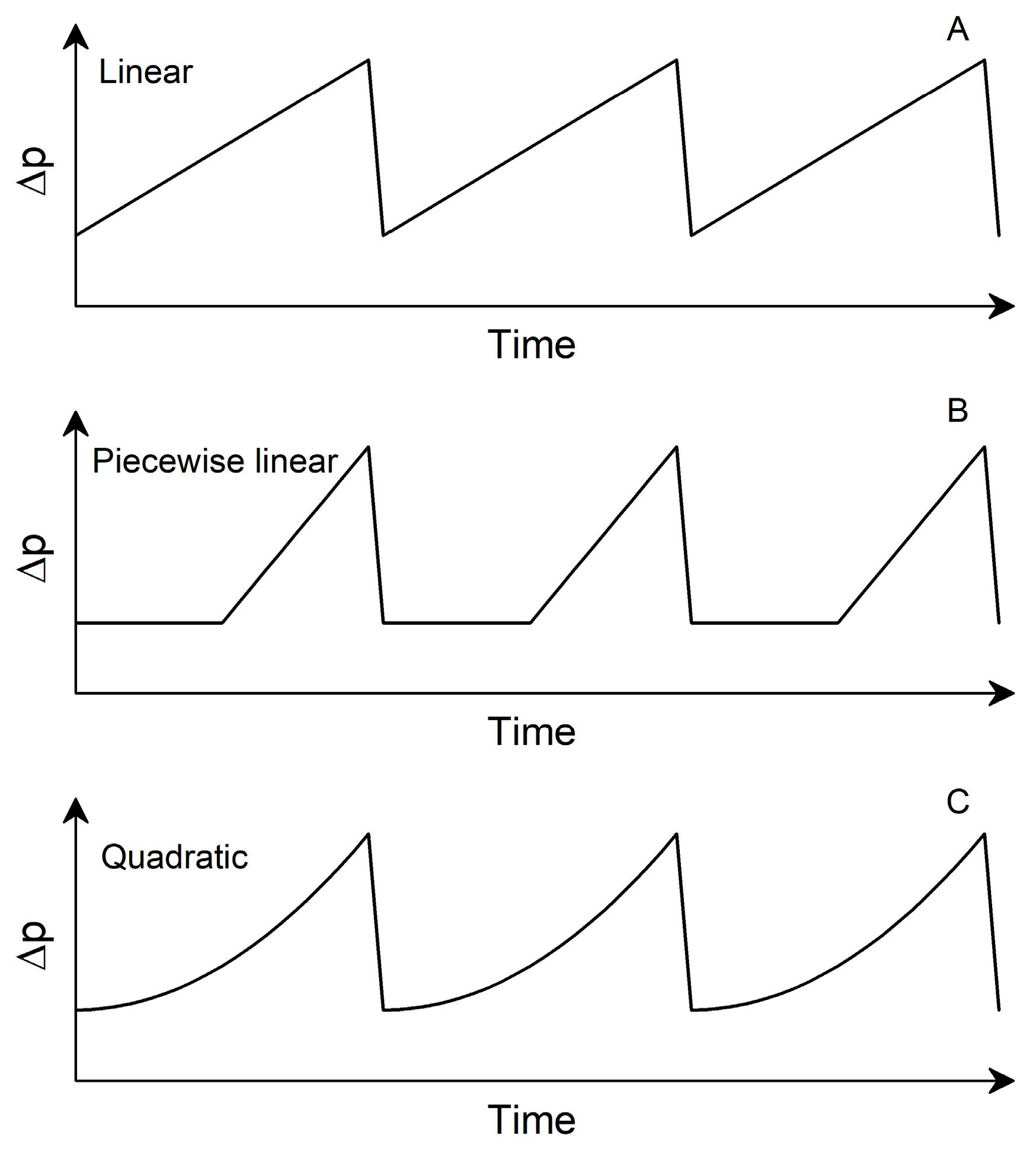
2.3. Filtration Cycles

One filtration cycle included one filtration period and one backwashing period. Filter pressure drop values for both filtration and backwashing periods were defined as $\mathsf{\Delta }{\mathrm{p}}_{\mathrm{F}}$ and $\mathsf{\Delta }{\mathrm{p}}_{\mathrm{B}}$, respectively. For simplicity, each period was assumed to start at zero time, so the duration of both filtration and backwashing regimes were ${\mathrm{t}}_{\mathrm{F}}$ and ${\mathrm{t}}_{\mathrm{B}}$, respectively. Note that both $\mathsf{\Delta }{\mathrm{p}}_{\mathrm{F}}$ and $\mathsf{\Delta }{\mathrm{p}}_{\mathrm{B}}$ were, in general, functions of time. The value of ${\mathrm{t}}_{\mathrm{F}}$ was determined from the condition that the filter pressure drop reached the end value $\mathsf{\Delta }{\mathrm{p}}_{\mathrm{e}}$ (i.e., $\mathsf{\Delta }{\mathrm{p}}_{\mathrm{F}}(\mathrm{t}={\mathrm{t}}_{\mathrm{F}})=\mathsf{\Delta }{\mathrm{p}}_{\mathrm{e}}$), which was a preset value above the initial (clean filter) pressure drop $\mathsf{\Delta }{\mathrm{p}}_0$ (i.e., $\mathsf{\Delta }{\mathrm{p}}_{\mathrm{F}}(\mathrm{t}=0)=\mathsf{\Delta }{\mathrm{p}}_0$),

$$\mathsf{\Delta }{\mathrm{p}}_{\mathrm{e}}=\mathsf{\Delta }{\mathrm{p}}_0+\mathsf{\Delta }{\mathrm{p}}_{\mathrm{s}}$$

(1)

with $\mathsf{\Delta }{\mathrm{p}}_{\mathrm{s}}$ as the setpoint value. Several authors have applied $\mathsf{\Delta }{\mathrm{p}}_{\mathrm{s}}$ = 50 × 10³ Pa [32,38,41,42], although different filter technologies may use other values.

The time span of the backwashing mode t_B was fixed, being independent of the values assumed for the volumetric flow rate Q_B or the filter pressure drop ${\mathsf{\Delta }\mathrm{p}}_{\mathrm{B}}$ for backwashing conditions. For convenience, the following dimensionless ratios were defined

$${\mathrm{x}}_{\mathrm{Q}}={\displaystyle \frac{{\mathrm{Q}}_{\mathrm{B}}}{{\mathrm{Q}}_{\mathrm{F}}}}$$

(2)

$${\mathrm{x}}_{\mathrm{p}}={\displaystyle \frac{{\mathsf{\Delta }\mathrm{p}}_{\mathrm{B}}}{{\mathsf{\Delta }\mathrm{p}}_0}}$$

(3)

since many previous studies report constant backwashing values ${\mathrm{Q}}_{\mathrm{B}}$ and ${\mathsf{\Delta }\mathrm{p}}_{\mathrm{B}}$ in addition to the filtration values for the volumetric flow rate ${\mathrm{Q}}_{\mathrm{F}}$ and initial pressure drop ${\mathsf{\Delta }\mathrm{p}}_0$. For example, ${\mathrm{x}}_{\mathrm{Q}}=1$ corresponds to filters whose nominal backwashing flow rate is equal to that for filtration, and ${\mathrm{x}}_{\mathrm{P}}=1$ to filters in which the backwashing pressure drop is equal to that in filtration mode with tap water (or, equivalently, to the pressure drop at the beginning of the filtration cycle).

On the other hand, the hydraulic energy required for both filtration ${\mathrm{E}}_{\mathrm{F}}$ and backwashing ${\mathrm{E}}_{\mathrm{B}}$ modes were calculated using

$${\mathrm{E}}_{\mathrm{i}}=\underset{0}{\overset{{\mathrm{t}}_{\mathrm{i}}}{\int }}{\mathrm{Q}}_{\mathrm{i}}\mathsf{\Delta }{\mathrm{p}}_{\mathrm{i}}\mathrm{d}\mathrm{t}\hspace{1em}\mathrm{for} \mathrm{i}=\mathrm{F},\mathrm{B}$$

(4)

where t is the time.

The volume of filtered V_F and backwashed V_B water was obtained from

$${\mathrm{V}}_{\mathrm{i}}=\underset{0}{\overset{{\mathrm{t}}_{\mathrm{i}}}{\int }}{\mathrm{Q}}_{\mathrm{i}}\mathrm{d}\mathrm{t}\hspace{1em}\mathrm{for} \mathrm{i}=\mathrm{F},\mathrm{B}.$$

(5)

Thus, the total values of hydraulic energy and water volume used for one cycle became ${\mathrm{E}}_{\mathrm{c}}={\mathrm{E}}_{\mathrm{F}}+{\mathrm{E}}_{\mathrm{B}}$ and ${\mathrm{V}}_{\mathrm{c}}={\mathrm{V}}_{\mathrm{F}}+{\mathrm{V}}_{\mathrm{B}}$, respectively.

2.3.1. Linear Behavior

The time evolution of the filter pressure drop in filtration mode $\mathsf{\Delta }{\mathrm{p}}_{\mathrm{F}}$ for the linear trend (Figure 1A) was expressed as

$$\mathsf{\Delta }{\mathrm{p}}_{\mathrm{F}}=\mathsf{\Delta }{\mathrm{p}}_0+{\mathsf{\beta }}_{\mathrm{l}}\mathrm{t}$$

(6)

with β_l being the slope and t being the time (t = 0 corresponds to the initial, clean filter conditions). The slope β_l is related to the retention rate of particles by the filter element, since this causes the continuous increase in the filter pressure drop. A total of 40 datasets published in [24,25,30,33,36] were fitted to Equation (6) with coefficients of determination R² > 0.909 and p-values for β_l < 0.001 (see Supplementary Information).

From Equations (1) and (6), the final time for the filtration mode read

$${\mathrm{t}}_{\mathrm{F}}={\displaystyle \frac{\mathsf{\Delta }{\mathrm{p}}_{\mathrm{s}}}{{\mathsf{\beta }}_{\mathrm{l}}}}.$$

(7)

For simplicity, the volumetric flow rate in filtration mode ${\mathrm{Q}}_{\mathrm{F}}$ was assumed constant as it occurs by using pumps with variable frequency drives that adjust to the demand [43]. The effect of this assumption was critically analyzed in the discussion section.

The first index calculated the hydraulic energy consumed in one cycle per unit volume of filtered water (i.e., usable water), which, from Equations (1)–(4) and (7), was

$${\displaystyle \frac{{\mathrm{E}}_{\mathrm{c}}}{{\mathrm{V}}_{\mathrm{F}}}}={\displaystyle \frac{\mathsf{\Delta }{\mathrm{p}}_{\mathrm{s}}}{2}}+\mathsf{\Delta }{\mathrm{p}}_0\left(1+{\mathrm{x}}_{\mathrm{Q}}{\mathrm{x}}_{\mathrm{p}}{\displaystyle \frac{{\mathsf{\beta }}_{\mathrm{l}}{\mathrm{t}}_{\mathrm{B}}}{\mathsf{\Delta }{\mathrm{p}}_{\mathrm{s}}}}\right).$$

(8)

Equation (8) is expressed in terms of three key parameters of the filtration mode: $\mathsf{\Delta }{\mathrm{p}}_0$, β_l, and $\mathsf{\Delta }{\mathrm{p}}_{\mathrm{s}}$. The latter (setpoint value) is recommended by manufacturers, though end users can freely modify it. The clean filter pressure drop $\mathsf{\Delta }{\mathrm{p}}_0$ only depends on the filter design once the operational conditions (i.e., volumetric flow rate) are fixed, whereas the slope β_l is affected by both the influent quality and the filter design. These two terms identify with each one of the two abovementioned strategies to improve filter designs (diminish initial pressure drop vs. prolong filtration time). Equation (8) also contains the three key parameters for backwashing: ${\mathrm{x}}_{\mathrm{Q}}$, ${\mathrm{x}}_{\mathrm{p}}$, and ${\mathrm{t}}_{\mathrm{B}}$, which were assumed constant. Note that Equation (8) is independent of the flow rate, since values are normalized per unit volume.

The second index calculated the ratio of filtered volume of water (usable water for irrigation) to total volume of water in the cycle, and was obtained from Equations (1), (2), and (5), being

$${\mathsf{\eta }}_{\mathrm{V}}={\displaystyle \frac{{\mathrm{V}}_{\mathrm{F}}}{{\mathrm{V}}_{\mathrm{c}}}}={\displaystyle \frac{1}{1+{\mathrm{x}}_{\mathrm{Q}}\frac{{\mathsf{\beta }}_{\mathrm{l}}{\mathrm{t}}_{\mathrm{B}}}{\mathsf{\Delta }{\mathrm{p}}_{\mathrm{s}}}}}$$

(9)

where ${\mathsf{\eta }}_{\mathrm{V}}$ represents the efficiency of water use in the filtration cycle. Note that neither of the $\mathsf{\Delta }{\mathrm{p}}_0$ nor ${\mathrm{x}}_{\mathrm{p}}$ terms appear in Equation (9).

2.3.2. Piecewise Linear Behavior

In the simplified piecewise linear behavior, the time evolution of the filter pressure drop in filtration mode $\mathsf{\Delta }{\mathrm{p}}_{\mathrm{F}}$ (Figure 1B) followed

$$\mathsf{\Delta }{\mathrm{p}}_{\mathrm{F}}=\left\{\begin{array}{cc}\mathsf{\Delta }{\mathrm{p}}_0& \mathrm{t}<{\mathrm{t}}_1\\ \mathsf{\Delta }{\mathrm{p}}_0+{\mathsf{\beta }}_{\mathrm{p}}\left(\mathrm{t}-{\mathrm{t}}_1\right)& \mathrm{t}\ge {\mathrm{t}}_1\end{array}\right.$$

(10)

with ${\mathsf{\beta }}_{\mathrm{p}}$ being the slope of the linear trend and t₁ the time at which the initial constant value begins to rise. As for β_l, the slope ${\mathsf{\beta }}_{\mathrm{p}}$ depends upon the rate at which particles are captured in the filter. In these filtration systems, there exists an initial period of length t₁ where the retention of particles does not substantially modify the pressure drop. This time is a fraction ${\mathrm{x}}_{\mathrm{T}}$ of the total filtration time ${\mathrm{t}}_{\mathrm{F}}$,

$${\mathrm{x}}_{\mathrm{T}}={\displaystyle \frac{{\mathrm{t}}_1}{{\mathrm{t}}_{\mathrm{F}}}},$$

(11)

meaning that (10) transforms into (6) for ${\mathrm{x}}_{\mathrm{T}}$ = 0.

Equation (10) was fitted to data in [21,22,23,31,37], with 43 datasets having coefficient of determination values R² > 0.937 and p-values for ${\mathsf{\beta }}_{\mathrm{p}}$ < 0.001. From Equations (1) and (10), the end time of the filtration regime was achieved using

$${\mathrm{t}}_{\mathrm{F}}={\displaystyle \frac{\mathsf{\Delta }{\mathrm{p}}_{\mathrm{s}}}{{\mathsf{\beta }}_{\mathrm{p}}(1-{\mathrm{x}}_{\mathrm{T}})}}.$$

(12)

The first index was obtained from Equations (1)–(4), (10), and (11), being

$${\displaystyle \frac{{\mathrm{E}}_{\mathrm{c}}}{{\mathrm{V}}_{\mathrm{F}}}}={\displaystyle \frac{\mathsf{\Delta }{\mathrm{p}}_{\mathrm{s}}}{2}}\left(1-{\mathrm{x}}_{\mathrm{T}}\right)+\mathsf{\Delta }{\mathrm{p}}_0\left(1+{\mathrm{x}}_{\mathrm{Q}}{\mathrm{x}}_{\mathrm{p}}{\displaystyle \frac{{\mathsf{\beta }}_{\mathrm{p}}{\mathrm{t}}_{\mathrm{B}}}{\mathsf{\Delta }{\mathrm{p}}_{\mathrm{s}}}}\left(1-{\mathrm{x}}_{\mathrm{T}}\right)\right)$$

(13)

which reduced to Equation (8) in the limit ${\mathrm{x}}_{\mathrm{T}}\to 0$, as it should. The limit ${\mathrm{x}}_{\mathrm{T}}\to 1$ is equivalent to ${\mathrm{t}}_1\to {\mathrm{t}}_{\mathrm{F}}$, meaning that the filtration system maintained the initial pressure throughout all of the filtration mode (i.e., ${\mathrm{E}}_{\mathrm{c}}/{\mathrm{V}}_{\mathrm{F}}=\mathsf{\Delta }{\mathrm{p}}_0$). From Equation (12), this limit was also equivalent to an infinite time in filtration mode.

By combining Equations (1), (2), (5), (10), and (11), the second index became

$${\mathsf{\eta }}_{\mathrm{V}}={\displaystyle \frac{{\mathrm{V}}_{\mathrm{F}}}{{\mathrm{V}}_{\mathrm{c}}}}={\displaystyle \frac{1}{1+{\mathrm{x}}_{\mathrm{Q}}\frac{{\mathsf{\beta }}_{\mathrm{p}}{\mathrm{t}}_{\mathrm{B}}}{\mathsf{\Delta }{\mathrm{p}}_{\mathrm{s}}}\left(1-{\mathrm{x}}_{\mathrm{T}}\right)}}$$

(14)

which converts into Equation (9) in the limit ${\mathrm{x}}_{\mathrm{T}}\to 0$, as expected. An ideal behavior is obtained in the limit ${\mathrm{x}}_{\mathrm{T}}\to 1$, since there is not a backwashing regime (infinite duration of the filtration mode from Equation (12)).

2.3.3. Quadratic Behavior

Finally, the pure quadratic behavior of the filter pressure drop in filtration mode $\mathsf{\Delta }{\mathrm{p}}_{\mathrm{F}}$ that follows the pattern in Figure 1C is calculated by

$$\mathsf{\Delta }{\mathrm{p}}_{\mathrm{F}}=\mathsf{\Delta }{\mathrm{p}}_0+{\mathsf{\beta }}_{\mathrm{q}}{\mathrm{t}}^2$$

(15)

with ${\mathsf{\beta }}_{\mathrm{q}}$ being the quadratic coefficient whose value varies depending on how particles are retained by the filtration system. Equation (15) fitted to R4 in Figure 3B and to 17 datasets in [21,30,31,37] provided values of the coefficient of determination R² > 0.907 and p-values for ${\mathsf{\beta }}_{\mathrm{q}}$ < 0.001.

From Equations (1) and (15), the end of the filtration mode was reached at time

$${\mathrm{t}}_{\mathrm{F}}=\sqrt{{\displaystyle \frac{\mathsf{\Delta }{\mathrm{p}}_{\mathrm{s}}}{{\mathsf{\beta }}_{\mathrm{q}}}}}.$$

(16)

As in the preceding cases, the first index was obtained from Equations (1)–(4) and, now, from (15), being

$${\displaystyle \frac{{\mathrm{E}}_{\mathrm{c}}}{{\mathrm{V}}_{\mathrm{F}}}}={\displaystyle \frac{\mathsf{\Delta }{\mathrm{p}}_{\mathrm{s}}}{3}}+\mathsf{\Delta }{\mathrm{p}}_0\left(1+{\mathrm{x}}_{\mathrm{Q}}{\mathrm{x}}_{\mathrm{p}}{\mathrm{t}}_{\mathrm{B}}\sqrt{{\displaystyle \frac{{\mathsf{\beta }}_{\mathrm{q}}}{\mathsf{\Delta }{\mathrm{p}}_{\mathrm{s}}}}}\right).$$

(17)

Finally, the second index followed from Equations (1), (2), (5), and (15), is

$${\mathsf{\eta }}_{\mathrm{V}}={\displaystyle \frac{{\mathrm{V}}_{\mathrm{F}}}{{\mathrm{V}}_{\mathrm{c}}}}={\displaystyle \frac{1}{1+{\mathrm{x}}_{\mathrm{Q}}{\mathrm{t}}_{\mathrm{B}}\sqrt{\frac{{\mathsf{\beta }}_{\mathrm{q}}}{\mathsf{\Delta }{\mathrm{p}}_{\mathrm{s}}}}}}.$$

(18)

Indeed, the water use efficiency index Equations (9), (14), and (18) reduce to

$${\mathsf{\eta }}_{\mathrm{V}}={\displaystyle \frac{{\mathrm{V}}_{\mathrm{F}}}{{\mathrm{V}}_{\mathrm{c}}}}={\displaystyle \frac{1}{1+\frac{{\mathrm{x}}_{\mathrm{Q}}{\mathrm{t}}_{\mathrm{B}}}{{\mathrm{t}}_{\mathrm{F}}}}}$$

(19)

with t_F being the corresponding end time of the filtration mode (Equations (7), (12) and (16)).

2.4. Supporting Data

Supporting data for the classification of Figure 1 were based on the analysis of Figure 3 and the collection of datasets from tables and figures of the filter pressure drop variation as a function of time published in [21,22,23,24,25,30,31,33,36,37]. These references were all related to filtration with drip irrigation using disc, screen, or porous media filters. A total of 108 different fits (45 with Equation (6), 45 with Equation (10), and 18 with Equation (15)) were applied to data (see Supplementary Information), neglecting the measurements of the first 30 s in [37] due to a very abrupt increase in the pressure drop, and focusing on data below 90% of the clogged pressure drop value in S-type curves (8 cases in [22], and 6 in [21]). In some conditions, the same data were fitted to both piecewise linear (10) and quadratic (15) equations, since a definite behavior was not identified. The coefficients of determination R² and the p-values for all the fits can be consulted in the Supplementary Information.

Table 1. Percentage of linear, piecewise, and quadratic trends for different filter types (see Supplementary Information).

Filter Type (Number)	Linear (%)	Piecewise Linear (%)	Quadratic (%)
Disc (39)	53.8	25.6	20.5
Porous media (23)	91.2	4.4	4.4
Screen (46)	6.5	73.9	19.6

summarizes the trend of the pressure drop versus time curve observed for each filter technology. The linear trend was clearly dominant in porous media elements. In disc filters, the linear pattern arose in half of the cases analyzed, with similar percentages of both piecewise linear and quadratic trends. However, the linear pattern was rare in screen filters, where the piecewise linear mode was the prevailing mode. Although the same filter technology might exhibit different behaviors, it was infrequent to observe pattern changes in the same type of study, indicating that the influent conditions played a relevant role in the determination of the pressure drop time evolution.

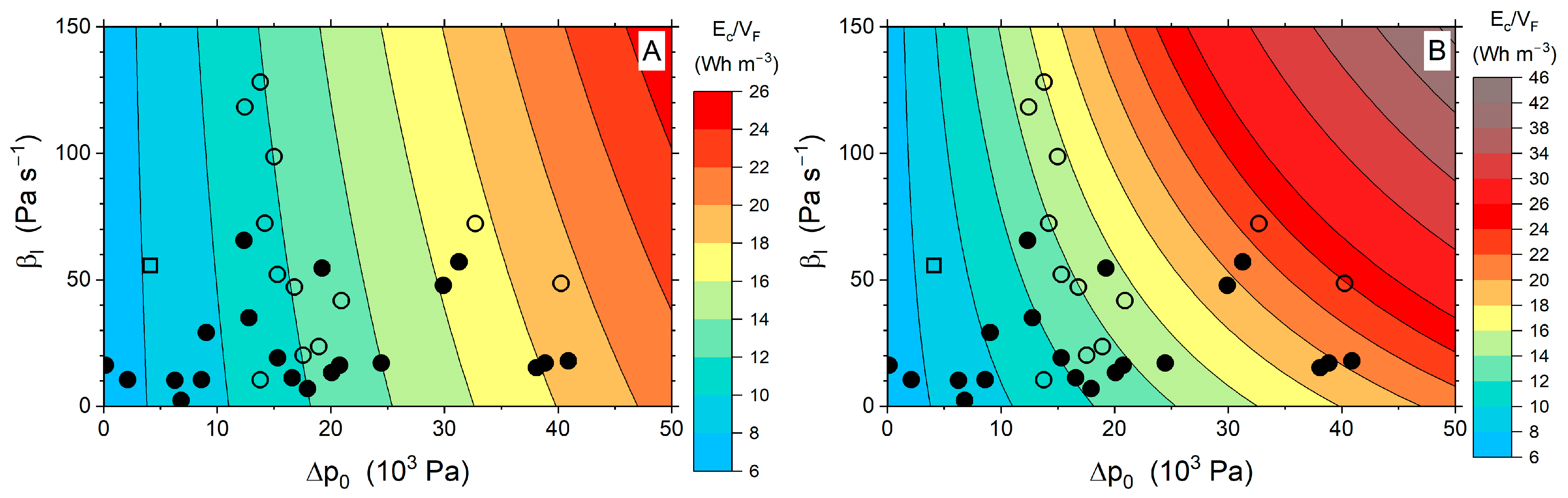
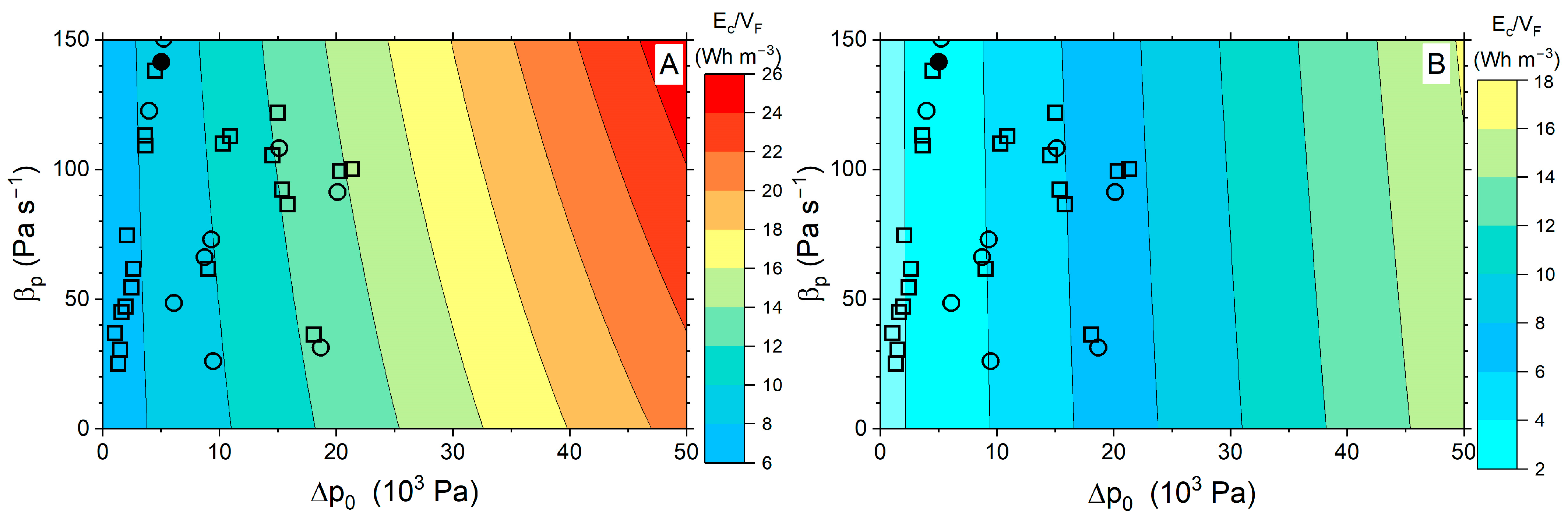
3. Results

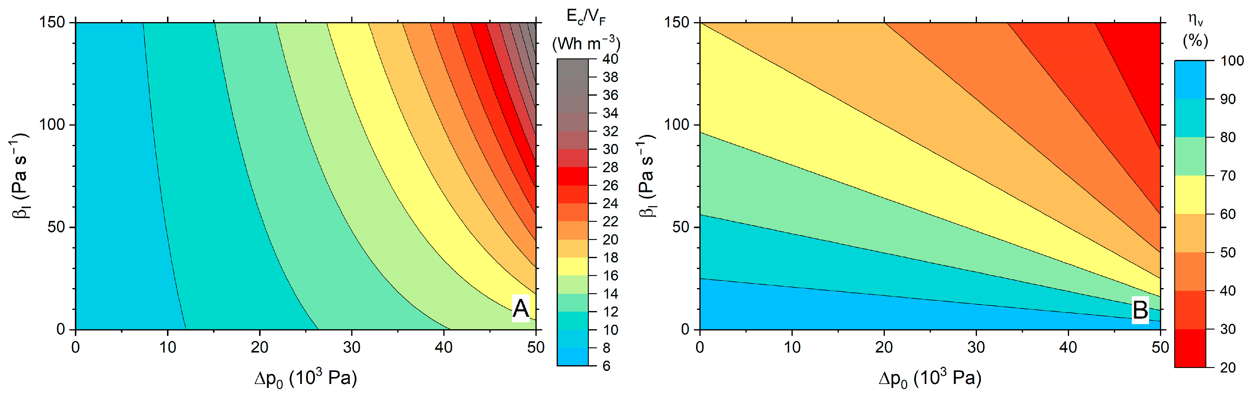
3.1. Linear Behavior

The energy consumed in one cycle divided by the volume of filtered water (${\mathrm{E}}_{\mathrm{c}}/{\mathrm{V}}_{\mathrm{F}}$) was evaluated by varying the two coefficients of the pressure drop vs. time linear curve (6) within a wide range of values that encompassed those expected from commercial filters of different technologies ($\mathsf{\Delta }{\mathrm{p}}_0$ from 0 to 50 × 10³ Pa, and β_l from 0.02 to 150 Pa s⁻¹). All cases assumed $\mathsf{\Delta }{\mathrm{p}}_{\mathrm{s}}$ = 50 × 10³ Pa, since this value is often recommended by manufacturers as a threshold setpoint [32]. Regarding the backwashing regime, two main parameters were fixed: the ratio of backwashing to filtration flow rate at ${\mathrm{x}}_{\mathrm{Q}}$ = 1.48, since it corresponded to the averaged recommendation from several manufacturers [40], and the duration of the backwashing regime at ${\mathrm{t}}_{\mathrm{B}}$ = 180 s, as it was used in [38]. The ratio of backwashing pressure drop to initial pressure drop $\mathsf{\Delta }{\mathrm{p}}_0$ value varied in Figure 4, being ${\mathrm{x}}_{\mathrm{p}}$ = 0.42 (Figure 4A), in agreement with experimental data of sand media filters [44], or ${\mathrm{x}}_{\mathrm{p}}$ = 2.0 (Figure 4B).

A strong influence of $\mathsf{\Delta }{\mathrm{p}}_0$ on ${\mathrm{E}}_{\mathrm{c}}/{\mathrm{V}}_{\mathrm{F}}$ was found, particularly for those scenarios with low ${\mathsf{\beta }}_{\mathrm{l}}$ values. For example, at $\mathsf{\Delta }{\mathrm{p}}_0$ = 15 × 10³ Pa and ${\mathsf{\beta }}_{\mathrm{l}}$ = 9 Pa s⁻¹, a 5% decrease in $\mathsf{\Delta }{\mathrm{p}}_0$ led to a decrease in ${\mathrm{E}}_{\mathrm{c}}/{\mathrm{V}}_{\mathrm{F}}$ of 1.90% (Figure 4A) or 1.98% (Figure 4B), whereas a 5% decrease in ${\mathsf{\beta }}_{\mathrm{l}}$ reduced ${\mathrm{E}}_{\mathrm{c}}/{\mathrm{V}}_{\mathrm{F}}$ by 0.04% (Figure 4A) or 0.17% (Figure 4B) only. From Equation (8), the β_l coefficient only affected the term related to the backwashing mode, whose reduction tends to minimize ${\mathrm{E}}_{\mathrm{c}}/{\mathrm{V}}_{\mathrm{F}}$ for fixed values of $\mathsf{\Delta }{\mathrm{p}}_0$ and $\mathsf{\Delta }{\mathrm{p}}_{\mathrm{s}}$. Indeed, the effect of the backwashing parameters ${\mathrm{x}}_{\mathrm{Q}}$, ${\mathrm{x}}_{\mathrm{p}}$, and ${\mathrm{t}}_{\mathrm{B}}$ on ${\mathrm{E}}_{\mathrm{c}}/{\mathrm{V}}_{\mathrm{F}}$ was essentially the same, as they solely contributed in the product form ${\mathrm{x}}_{\mathrm{Q}}{\mathrm{x}}_{\mathrm{p}}{\mathrm{t}}_{\mathrm{B}}$ to the increase in the index (weighted by β_l and the $\mathsf{\Delta }{\mathrm{p}}_0/\mathsf{\Delta }{\mathrm{p}}_{\mathrm{s}}$ factor). Thus, any equal variation proposed in ${\mathrm{x}}_{\mathrm{Q}}$, ${\mathrm{x}}_{\mathrm{p}}$, or ${\mathrm{t}}_{\mathrm{B}}$ produced the same effects on ${\mathrm{E}}_{\mathrm{c}}/{\mathrm{V}}_{\mathrm{F}}$, provided that all other coefficients remain the same.

However, ${\mathrm{x}}_{\mathrm{Q}}$ variations are limited by common operational conditions. From manufacturers’ datasets of pressurized filters for drip irrigation, it is unlikely that ${\mathrm{x}}_{\mathrm{Q}}$ > 1.5 [44], whereas the condition ${\mathrm{x}}_{\mathrm{Q}}$ ≈ 1 recently appeared as a plausible goal for a new filter design [40], although values of ${\mathrm{x}}_{\mathrm{Q}}$ slightly below 1 were also used in tests of commercial media filters [17]. On the other hand, the backwashing time ${\mathrm{t}}_{\mathrm{B}}$ may present substantial variations around the value chosen in Figure 4 (180 s as in [32]). For example, in media filters, a value of ${\mathrm{t}}_{\mathrm{B}}$ = 120 s was applied in [17], and varied between 90 and 180 s in practical recommendations [45], although it reached 900 s in laboratory analyses of commercial units [46]. The backwashing time is particularly dependent on the filter technology, since screen filters may require shorter backwashing times than media ones; former optimization studies have suggested values between 30 and 45 s only [34]. Regarding the ${\mathrm{x}}_{\mathrm{p}}$ ratio, it can also present a high variability, being ${\mathrm{x}}_{\mathrm{p}}$ = 0.42 in published datasets from a laboratory porous media filter [44], but ${\mathrm{x}}_{\mathrm{p}}$ ≈ 2.0, or even greater, in some commercial units [17]. In screen filters, $\mathsf{\Delta }{\mathrm{p}}_{\mathrm{B}}$ may actually vary with time in runs with relevant clogging, since the backwash initiates with strong retention [34]. However, this effect suddenly disappears, and ${\mathrm{x}}_{\mathrm{p}}$ ≈ 1.2 or 1.3 [34]. In automatic commercial filters, the main cause of this 5-fold increase in ${\mathrm{x}}_{\mathrm{p}}$ can be explained by the effect of three-way valves that operate in the backwashing mode, since, in some cases, they can produce very high energy losses [17].

The backwashing terms in Equation (8) were weighted by the factor $\mathsf{\Delta }{\mathrm{p}}_0/\mathsf{\Delta }{\mathrm{p}}_{\mathrm{s}}$, meaning that rising the setpoint value $\mathsf{\Delta }{\mathrm{p}}_{\mathrm{s}}$ weakened their influence on ${\mathrm{E}}_{\mathrm{c}}/{\mathrm{V}}_{\mathrm{F}}$. This effect was directly linked to the prolongation of the filtration mode, not because of having a milder slope ${\mathsf{\beta }}_{\mathrm{l}}$ in Equation (6), but simply because of fixing a higher threshold value for $\mathsf{\Delta }{\mathrm{p}}_{\mathrm{e}}$.

In terms of water use efficiency, the pressure drop value $\mathsf{\Delta }{\mathrm{p}}_0$ for clean conditions did not have any incidence in ${\mathsf{\eta }}_{\mathrm{V}}$, since it did not alter the time span of the filtration mode. Only two parameters that characterized the filtration mode (${\mathsf{\beta }}_{\mathrm{l}}$ and $\mathsf{\Delta }{\mathrm{p}}_{\mathrm{s}}$), and two parameters that characterized the backwashing one (${\mathrm{x}}_{\mathrm{Q}}$ and ${\mathrm{t}}_{\mathrm{B}}$), played a role in ${\mathsf{\eta }}_{\mathrm{V}}$. The pressure drop during backwashing was also irrelevant for ${\mathsf{\eta }}_{\mathrm{V}}$. Therefore, the analysis was carried out fixing $\mathsf{\Delta }{\mathrm{p}}_{\mathrm{s}}$ = 50 × 10³ Pa and varying ${\mathsf{\beta }}_{\mathrm{l}}$ with different values of ${\mathrm{x}}_{\mathrm{Q}}$ and ${\mathrm{t}}_{\mathrm{B}}$ (Figure 5). The effect of ${\mathsf{\beta }}_{\mathrm{l}}$ on ${\mathsf{\eta }}_{\mathrm{V}}$ was more important at low values of ${\mathsf{\beta }}_{\mathrm{l}}$, being very sensitive to variations in the ${\mathrm{x}}_{\mathrm{Q}}{\mathrm{t}}_{\mathrm{B}}$ product. For example, with $\mathsf{\Delta }{\mathrm{p}}_{\mathrm{s}}$ = 50 × 10³ Pa and ${\mathsf{\beta }}_{\mathrm{l}}$ = 9 Pa s⁻¹, an increase in the backwashing time from 180 s to 360 s led to a decrease in water use efficiency from 95% to 91%. For the very same variation in backwashing times, a more dramatic decrease in water use efficiency was observed with ${\mathsf{\beta }}_{\mathrm{l}}$ = 80 Pa s⁻¹, since it dropped from 70% to 54%. Therefore, the duration of the backwashing time must be carefully selected to avoid an excessive amount of non-filtered water, especially in those filters with high pressure drop slopes as a function of time. Note that in some drip irrigation installations, the water used for backwashing is not recovered, being irreversibly lost.

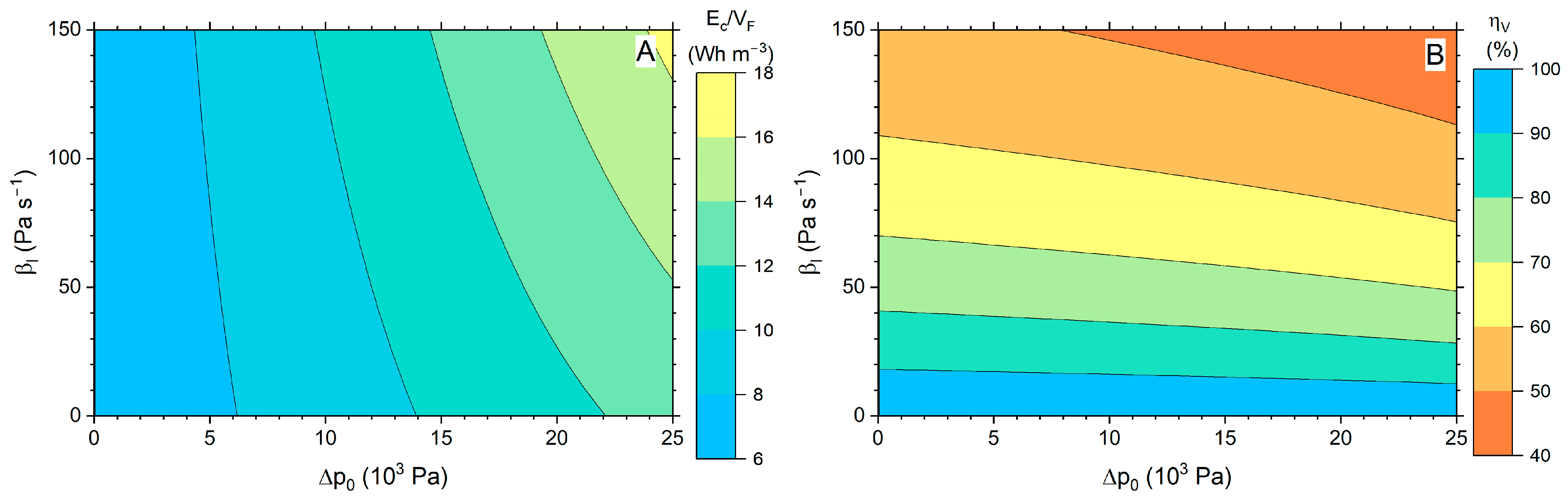
3.2. Piecewise Linear Behavior

For a filtration system with a piecewise linear behavior (10), the index ${\mathrm{E}}_{\mathrm{c}}/{\mathrm{V}}_{\mathrm{F}}$ was mainly affected by $\mathsf{\Delta }{\mathrm{p}}_0$, with the slope ${\mathsf{\beta }}_{\mathrm{p}}$ being of less importance than in the preceding case as ${\mathrm{x}}_{\mathrm{T}}$ increased (Figure 6). In comparison with the linear behavior (i.e., ${\mathrm{x}}_{\mathrm{T}}$ = 0), the energy use efficiency ${\mathrm{E}}_{\mathrm{c}}/{\mathrm{V}}_{\mathrm{F}}$ substantially improved with ${\mathrm{x}}_{\mathrm{T}}$ as the filtration system spent more time in conditions close to those of the initial of the cycle. Therefore, for this type of filtration behavior, the recommended design action to reduce the energy consumption per unit of filtered volume must concentrate on diminishing the $\mathsf{\Delta }{\mathrm{p}}_0$ value.

The water use efficiency index was less sensitive to changes in the slope of the piecewise linear function of the filtration system as ${\mathrm{x}}_{\mathrm{T}}$ increased, as was clearly observed when comparing Figure 7 (${\mathrm{x}}_{\mathrm{T}}$ = 0.8) with Figure 5 (${\mathrm{x}}_{\mathrm{T}}$ = 0). Nevertheless, the effect of the backwashing terms ${\mathrm{x}}_{\mathrm{Q}}$ and ${\mathrm{t}}_{\mathrm{B}}$ still remained, although not as pronounced as in the full linear behavior.

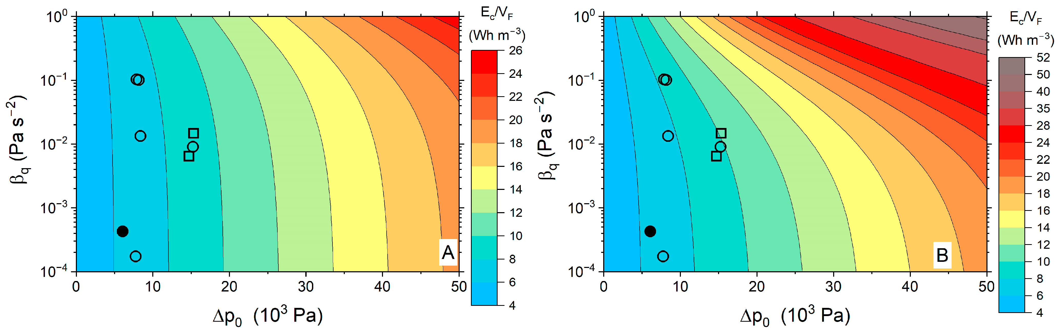
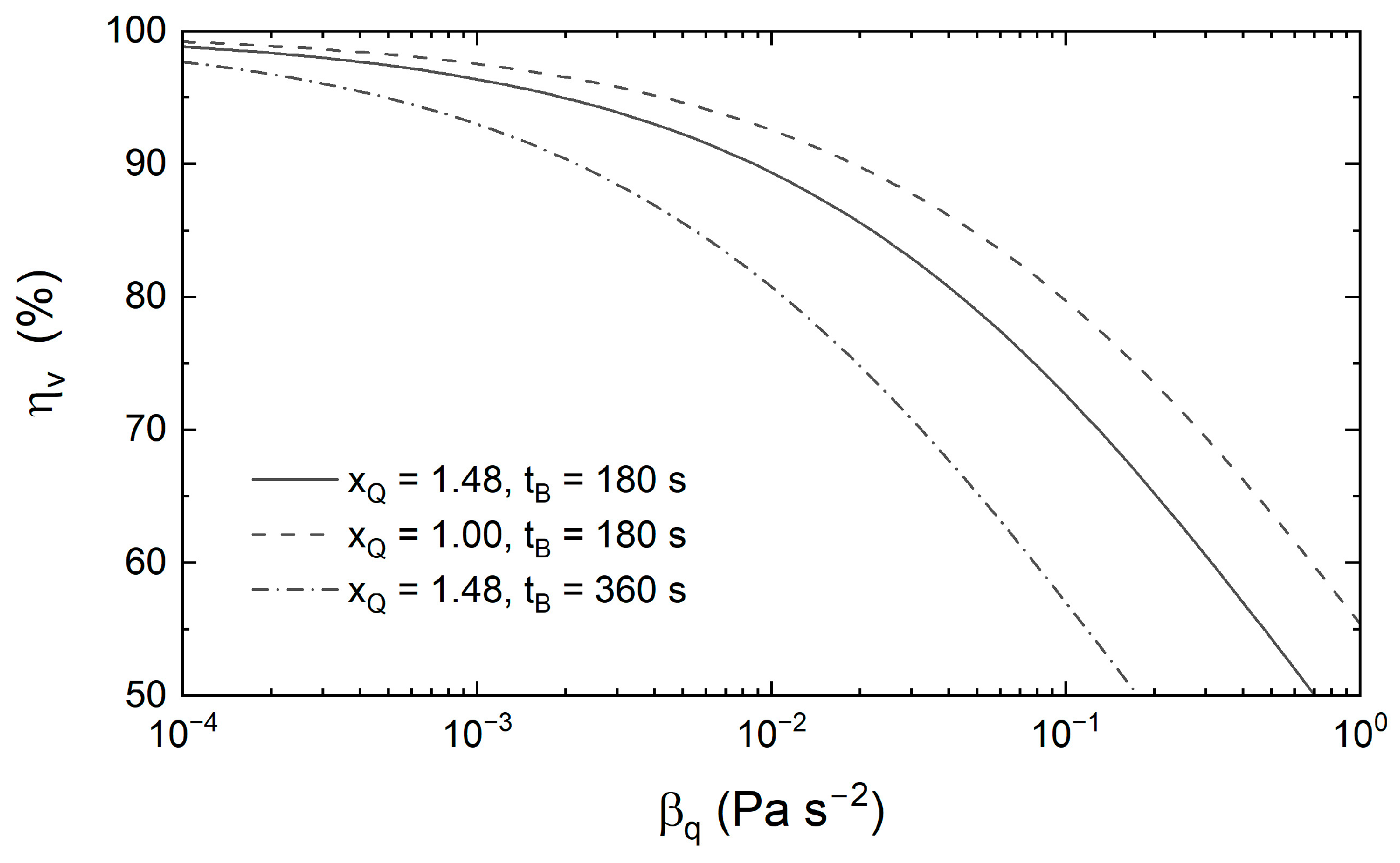
3.3. Quadratic Behavior

Finally, the analysis of real filtration systems with a pure quadratic type behavior of the filter pressure drop variation as a function of time revealed a very wide range of possible values for the coefficient ${\mathsf{\beta }}_{\mathrm{q}}$ (see dots in Figure 8). In contrast, values of the initial filter pressure drop (clean filter conditions) ${\mathsf{\Delta }\mathrm{p}}_0$ were in the lower range of those datasets analyzed for the two previous behaviors (<10⁴ Pa). The energy use efficiency expressed as ${\mathrm{E}}_{\mathrm{c}}/{\mathrm{V}}_{\mathrm{F}}$ exposed a low sensitivity to changes in ${\mathsf{\beta }}_{\mathrm{q}}$ in systems with low values of this parameter. However, in the upper zone of reported values for ${\mathsf{\beta }}_{\mathrm{q}}$, this term may become the prominent one in terms of the influence on the energy use efficiency as ${\mathsf{\Delta }\mathrm{p}}_0$ increases. Therefore, the recommended design route for these scenarios should not only involve a reduction in ${\mathsf{\Delta }\mathrm{p}}_0$ but also in ${\mathsf{\beta }}_{\mathrm{q}}$.

High values of ${\mathsf{\beta }}_{\mathrm{q}}$ were equivalent to small filtration times, which did not penalize in excess the energy use efficiency. However, they did highly compromise the water use efficiency, with very low values of ${\mathsf{\eta }}_{\mathrm{V}}$ (Figure 9). As in the preceding cases, the effects of ${\mathrm{x}}_{\mathrm{Q}}$ and ${\mathrm{t}}_{\mathrm{B}}$ also appeared, gaining in importance as the ${\mathsf{\beta }}_{\mathrm{q}}$ value increased.

4. Discussion

In some real-world applications, the sediment concentration of water may substantially vary with time, as was detected in R1, Figure 3A. In this scenario, the actual $\mathsf{\Delta }{\mathrm{p}}_{\mathrm{F}}\left(\mathrm{t}\right)$ functions may be more complex than simple linear (6), piecewise linear (10), and quadratic (15) expressions. For example, the linear behavior may transform into a sequential linear with different slopes. In any case, Equations (4) and (5) are still valid, and the methodology described here could also be applied for different $\mathsf{\Delta }{\mathrm{p}}_{\mathrm{F}}\left(\mathrm{t}\right)$ functions. Nevertheless, small variations in the inlet flow properties are not expected to modify the conclusions reported here.

In addition, another limitation of the present study is the assumption of constant volumetric flow rate. This fixed delivery requires continuous adaptation of the pump performance curve to match the system characteristics [47], which can be achieved with variable frequency drives [43]. Although the adoption of this technology has many advantages [48], there are many pressurized drip irrigation installations that operate with constant speed pumps. In these cases, the pump performance curve can be assimilated to a parabolic curve in terms of the volumetric flow rate $\mathrm{Q}$, being $\mathsf{\Delta }{\mathrm{p}}_{\mathrm{P}}=a-b{\mathrm{Q}}^2$ with $\mathsf{\Delta }{\mathrm{p}}_{\mathrm{P}}$ being the pump’s head and $a$ and $b$ being positive constants [47]. Thus, the condition $\mathsf{\Delta }{\mathrm{p}}_{\mathrm{P}}=\mathsf{\Delta }{\mathrm{p}}_{\mathrm{F}}$ for the filtration mode implies a flow reduction from ${\mathrm{Q}}_0=\sqrt{\left(a-\mathsf{\Delta }{\mathrm{p}}_0\right)/b}$ at the start to ${\mathrm{Q}}_{\mathrm{e}}=\sqrt{\left(a-\mathsf{\Delta }{\mathrm{p}}_{\mathrm{e}}\right)/b}$ at the end of the filtration regime (see Equation (1)). For the linear behavior pattern (6), by fixing values of backwashing parameters ${\mathrm{t}}_{\mathrm{B}}$, ${\mathrm{x}}_{\mathrm{Q}}$, and ${\mathrm{x}}_{\mathrm{p}}$, and by assuming $a$ and $b$ values such that ${\mathrm{Q}}_{\mathrm{e}}/{\mathrm{Q}}_0=$ 0.5, the solution was very similar to that reported in Section 3.1. This was a consequence of considering pump performance curves specifically fitted to each one of the scenarios ($\mathsf{\Delta }{\mathrm{p}}_0$ and $\mathsf{\Delta }{\mathrm{p}}_{\mathrm{e}}$) analyzed. However, results substantially varied when working with a unique pump performance curve (defined for $\mathsf{\Delta }{\mathrm{p}}_0$ = 10 × 10³ Pa and $\mathsf{\Delta }{\mathrm{p}}_{\mathrm{s}}$ = 50 × 10³ Pa) for all the scenarios studied. In this case, the pump could not cope with large values of $\mathsf{\Delta }{\mathrm{p}}_0$ (see Figure 10), but for those in which it produced feasible values, the ${\mathsf{\beta }}_{\mathrm{l}}$ term had a larger influence on the energy use efficiency (Figure 10A) than that observed with variable speed pumps (Figure 4A). The effect of reducing the flow rate, especially for long cycles (${\mathsf{\beta }}_{\mathrm{l}}$ low), led to slightly better values of energy use efficiency in comparison with Section 3.1, but highly penalized the water use efficiency (Figure 10B) that, now, was also dependent on the $\mathsf{\Delta }{\mathrm{p}}_0$ value. This was caused by the reduction in filtered water volume produced by the continuous decrease in flow rate.

On the other hand, modifications of the setpoint value $\mathsf{\Delta }{\mathrm{p}}_{\mathrm{s}}$ affected the previous results in the form of being less (more) sensitive to changes in β_l as $\mathsf{\Delta }{\mathrm{p}}_{\mathrm{s}}$ increased (decreased). In this sense, the larger the $\mathsf{\Delta }{\mathrm{p}}_{\mathrm{s}}$ value, the better the hydraulic energy use efficiency.

A different approach than (1) to obtain the condition for the end of the filtration cycle $\mathsf{\Delta }{\mathrm{p}}_{\mathrm{e}}$ was to set a given value irrespective of the value of the initial pressure drop $\mathsf{\Delta }{\mathrm{p}}_0$. The consequences of using a fixed value for $\mathsf{\Delta }{\mathrm{p}}_{\mathrm{e}}$ (i.e., set to 60 × 10³ Pa for convenience) were examined for the linear behavior (Figure 11). It was clearly observed that for low β_l conditions and large $\mathsf{\Delta }{\mathrm{p}}_0$ values, the hydraulic energy use efficiency was improved in comparison with Figure 4A, whereas for high β_l values it substantially worsened. This behavior could be explained by the ${\mathrm{E}}_{\mathrm{c}}/{\mathrm{V}}_{\mathrm{F}}$ index (8), expressed in the form

$${\displaystyle \frac{{\mathrm{E}}_{\mathrm{c}}}{{\mathrm{V}}_{\mathrm{F}}}}=\mathsf{\Delta }{\mathrm{p}}_0+{\displaystyle \frac{\mathsf{\Delta }{\mathrm{p}}_{\mathrm{e}}-\mathsf{\Delta }{\mathrm{p}}_0}{2}}+{\displaystyle \frac{{\mathrm{x}}_{\mathrm{Q}}{\mathrm{x}}_{\mathrm{p}}{\mathsf{\beta }}_{\mathrm{l}}{\mathrm{t}}_{\mathrm{B}}\mathsf{\Delta }{\mathrm{p}}_0}{\mathsf{\Delta }{\mathrm{p}}_{\mathrm{e}}-\mathsf{\Delta }{\mathrm{p}}_0}} .$$

(20)

where the pressure difference between the end and the initial times in filtration mode $\mathsf{\Delta }{\mathrm{p}}_{\mathrm{e}}-\mathsf{\Delta }{\mathrm{p}}_0$ was constant (=$\mathsf{\Delta }{\mathrm{p}}_{\mathrm{s}}$) in Section 3.1, and variable with $\mathsf{\Delta }{\mathrm{p}}_0$ when fixing the $\mathsf{\Delta }{\mathrm{p}}_{\mathrm{e}}$ value instead of the $\mathsf{\Delta }{\mathrm{p}}_{\mathrm{s}}$ one. Thus, as $\mathsf{\Delta }{\mathrm{p}}_0$ increased, $\mathsf{\Delta }{\mathrm{p}}_{\mathrm{e}}-\mathsf{\Delta }{\mathrm{p}}_0$ decreased, reducing the contribution of the second term on the right-hand side of Equation (20) and increasing that of the last term. However, the latter only took relevance for high values of β_l (i.e., at short times of the filtration regime), as observed in Figure 11A. The strategy of working with a fixed $\mathsf{\Delta }{\mathrm{p}}_{\mathrm{e}}$ value had a pronounced effect on the water use efficiency (Figure 11B). In general, as $\mathsf{\Delta }{\mathrm{p}}_0$ increased, the water use efficiency decreased, since now not only β_l but also $\mathsf{\Delta }{\mathrm{p}}_0$ modified the filtration time value. The higher the $\mathsf{\Delta }{\mathrm{p}}_0$, the lower the ${\mathrm{t}}_{\mathrm{F}}$, and, as in previous discussions, a reduction in the filtration time directly emphasized the role of the backwashing regime in the complete filtration cycle, which decreased water use efficiency.

Another different approach to set the end value of the filtration process $\mathsf{\Delta }{\mathrm{p}}_{\mathrm{e}}$ was to consider a proportional relationship with respect to the initial pressure drop value, $\mathsf{\Delta }{\mathrm{p}}_{\mathrm{e}}=\mathrm{k}\mathsf{\Delta }{\mathrm{p}}_0$, with k being a constant greater than 1. In order to illustrate the consequences of applying this condition to filtration systems with a linear behavior (6), a value of k = 8.9 was chosen corresponding to the average value from Figure 3B. The β_l term had a very small impact on the energy use efficiency (Figure 12A) but a substantial one on the water use efficiency (Figure 12B) due to its weight in the determination of the filtration time, now being ${\mathrm{t}}_{\mathrm{F}}=\left(\mathrm{k}-1\right)\mathsf{\Delta }{\mathrm{p}}_0/{\mathsf{\beta }}_{\mathrm{l}}$. Note that, in opposition to the previous analysis, the time span of the filtration mode increased with $\mathsf{\Delta }{\mathrm{p}}_0$, being the reason for the change in the slope sign of the contour lines of Figure 12B in comparison with Figure 11B.

Additional strategies based on limiting the time instead of pressure to define a filtration cycle in pressurized filters for drip irrigation have also been reported [49]. However, many filter manufacturers rely on differential pressure sensors to automate the sequence of filtration cycles [50], which suggests that pressure is the main variable to focus on in this process. In comparison with previous studies of pressurized filters for drip irrigation, very few analyzed the consequences of modifying the operational conditions (including design modifications) on both energy and water use efficiency. For example, values of energy consumption per unit of filtered volume of water similar to those reported here were obtained by [42] with a particle retention model, although the contribution of the backwashing regime was ignored. Indeed, the backwashing process is pointed out as fundamental for the energy efficiency of irrigation systems [16], since it is responsible for restoring the filter to its initial (low pressure difference) conditions, which does not always occur [41]. Related with the water use efficiency, values above 98.5% with media, screen, and discs filters installed in drip irrigation systems have been reported [41], which, although very high, may still involve large losses of water volumes. Shi et al. [14] tackled this issue by finding the optimum time in the filter pressure drop vs. time curve to trigger the backwashing regime in terms of water use efficiency. The commercial screen filter that they analyzed followed a piecewise linear trend and the optimum time took place almost at the beginning of the ascending curve [14]. This filtration pattern was equivalent to scenarios where ${\mathrm{x}}_{\mathrm{T}}$ is chosen close to 1 in Equation (1), which here were confirmed to be the most advantageous (see Section 3.2). Future studies may focus on determining not only the optimum time but also the optimum mechanism (i.e., threshold pressure, threshold time, etc.) to trigger the backwashing mode, which could be decided with a combination of intelligent control algorithms. Finally, it should be noted that the analyses of the energy use efficiency presented here were limited to the hydraulic contribution only. Detailed economic performance should include data such as initial investment, maintenance costs, etc. that were out of the scope of the present study.

5. Conclusions

The analysis of a pressurized filtration system for drip irrigation based on the time evolution pattern of the filter pressure drop was an innovative, simple approach that provided insight into the effects of changing its characteristic parameters on increasing hydraulic energy and water use efficiencies.

In terms of improving the hydraulic energy consumption in a cycle per unit of filtered water volume, the following apply:

• It is better to propose a redesign that decreases the filter pressure drop with tap water ${\mathsf{\Delta }\mathrm{p}}_0$ than another that extends the duration of the filtration cycle ${\mathrm{t}}_{\mathrm{F}}$.
• The effect of the backwashing regime appears as a product of three contributions: (1) volumetric flow rate ${\mathrm{Q}}_{\mathrm{B}}$ normalized by its filtration value, (2) filter pressure drop ${\mathsf{\Delta }\mathrm{p}}_{\mathrm{B}}$ normalized by the initial value in filtration mode, and (3) backwashing time span t_B. All of these three terms clearly depend on the filter design, although the type and concentration of particles may also affect them.
• High pressure backwashing methods are only recommended when associated with very low backwashing times. In the case that high pressure procedures become inevitable for backwashing, designs that prolong the duration of the filtration cycle may be beneficial in terms of energy consumption, although it is still more advisable to reduce the ${\mathsf{\Delta }\mathrm{p}}_0$ value.

In terms of improving the water use efficiency:

• The main filtration parameter is the slope of the $\mathsf{\Delta }{\mathrm{p}}_{\mathrm{F}}\left(\mathrm{t}\right)$ function, with a lower slope corresponding to a higher water use efficiency.
• ${\mathsf{\Delta }\mathrm{p}}_0$ and ${\mathsf{\Delta }\mathrm{p}}_{\mathrm{B}}$ values are irrelevant.
• The backwashing volumetric flow rate ${\mathrm{Q}}_{\mathrm{B}}$ normalized by its filtration value and the duration time for backwashing t_B are the unique backwashing parameters that contribute to variations in the water use efficiency.

Most likely, the duration of the backwashing process is the one that, from the design point of view, could experience the largest variation, except for those filtration systems that present a clear imbalance between filtration and backwashing flow rates (as occurred in some media filters).

The previous conclusions were based on observations from linear, piecewise linear, and quadratic behaviors using a variable speed pump and a setpoint condition driven by the pressure variation between the initial time and the end time. However, systems with constant speed pumps, and/or with setpoint conditions triggered by reaching a given pressure drop value, present water use efficiency figures that critically depend on the ${\mathsf{\Delta }\mathrm{p}}_0$ value.

The global approach developed offers valuable information for making decisions about the preferred changes in design and operation of pressurized filters for drip irrigation with the purpose of improving hydraulic energy and water use efficiency. In light of the results found, the recommended design actions are those that decrease the ${\mathsf{\Delta }\mathrm{p}}_0$ value (increase energy efficiency) and reduce either Q_B or t_B (increase water use efficiency).

References

- World Water Assessment Programme (UNESCO WWAP). The United Nations World Water Development Report 2017. In Wastewater: The Untapped Resource; UNESCO: Paris, France, 2017. [Google Scholar]
- National Plan for Wastewater Treatment, Sanitation, Efficiency, Savings and Reuse. General Water Directorate; Secretary of State for the Environment; Spanish Ministry for Ecological Transition and the Demographic Challenge, 2021. Available online: https://www.miteco.gob.es/content/dam/miteco/es/agua/temas/planificacion-hidrologica/dsear_plan_book_english_tcm30-538717.pdf (accessed on 10 March 2025).
- Doeser, B. Water policy under the European Grean Deal. In State Play and Key Challenges Ahead; Water Days 2021 Symposium: Lubljana, Slovenia, 2021. [Google Scholar]
- Hristov, J.; Barreiro-Hurle, J.; Salputra, G.; Blanco, M.; Witzke, P. Reuse of treated water in European agriculture: Potential to address water scarcity under climate change. Agric. Water Manag. 2021, 251, 106872. [Google Scholar] [CrossRef]
- Abi Saab, M.T.; Jomaa, I.; El Hage, R.; Skaf, S.; Fahed, S.; Rizk, Z.; Massaad, R.; Romanos, D.; Khairallah, Y.; Azzi, V.; et al. Are fresh water and reclaimed water safe for vegetable irritation? Empirical evidence from Lebanon. Water 2022, 14, 1437. [Google Scholar] [CrossRef]
- Ministerio de Agricultura, Pesa y Alimentación, 2024. Encuesta Sobre Superficies y Rendimientos de Cultivos. Análisis de Los Regadíos en España. 2023. Available online: https://www.mapa.gob.es/es/estadistica/temas/estadisticas-agrarias/boletin20231_tcm30-690544.pdf (accessed on 10 March 2025).
- Instituto Nacional de Estadística. Encuesta Sobre el uso del Agua en el Sector Agrario 2018 Estadísticas Sobre Agua. Available online: https://www.ine.es/dyngs/INEbase/operacion.htm?c=Estadistica_C&cid=1254736176839&menu=ultiDatos&idp=1254735976602 (accessed on 11 February 2025).
- ICID, International Comission on Irrigation and Drainage. Annual Report 2022-23. Available online: https://icid-ciid.org/icid_data_web/ar_2022-23.pdf (accessed on 10 February 2025).
- Trooien, T.P.; Hills, D.J. Application of Biological Effluent. In Microirrigation for Crop Production. Design, Operation and Management; Lamm, F.R., Ayars, J.E., Nakayama, F.S., Eds.; Elsevier: Amsterdam, The Netherlands, 2007; pp. 329–356. [Google Scholar]
- Lv, C.; Niu, W.; Du, Y.; Sun, J.; Dong, A.; Wu, M.; Mu, F.; Zhu, J.; Siddique, H.M. A meta-analysis of labyrinth channel emitter clogging characteristics under Yellow River water drip tape irrigation. Agric. Water Manag. 2024, 291, 108634. [Google Scholar] [CrossRef]
- Xiao, Y.; Ma, C.; Li, M.; Zhangzhong, L.; Song, P.; Li, Y. Interaction and adaptation of phosphorus fertilizer and calcium ion in drip irrigation systems: The perspective of emitter clogging. Agric. Water Manag. 2023, 282, 108269. [Google Scholar] [CrossRef]
- Zhang, W.; Cai, J.; Zhai, G.; Song, L.; Lv, M. Experimental study on the filtration characteristics and sediment distribution influencing factors of sand media filters. Water 2023, 15, 4303. [Google Scholar] [CrossRef]
- Xu, X.; Wang, Q.; Zhang, J.; Zong, R.; Liu, N.; Wang, Z. Experimental study of filtration performance of disc filter with discrete channel structure. J. Irrig. Drain. Eng. 2023, 149, 04023013. [Google Scholar] [CrossRef]
- Shi, K.; Liu, Z.; Xie, Y.; Li, M. Study on optimal start-up time and water usage volume of blowdown residue discharge of mesh filter. Water Supply 2021, 21, 2904–2915. [Google Scholar] [CrossRef]
- de Deus, F.P.; Testezlaf, R.; Mesquita, M. Assessment methodology of backwash in pressurized sand filters. Rev. Bras. Eng. Agric. Ambient. 2016, 20, 600–605. [Google Scholar] [CrossRef]
- de Deus, F.P.; Mesquita, M.; Salcedo Ramirez, J.C.; Testezlaf, R.; de Almeida, R.C. Hydraulic characterization of the backwash process in sand filters used in micro irrigation. Biosyst. Eng. 2020, 192, 188–198. [Google Scholar] [CrossRef]
- Burt, C.M. Hydraulics of Commercial Sand Media Filter Tanks Used for Agricultural Drip Irrigation. In ITRC Report No. R 10001. Irrigation Training and Research Center; California Polytechnic State University: San Luis Obispo, CA, USA, 2010. [Google Scholar]
- Tarjuelo, J.M.; Rodriguez-Diaz, J.A.; Abadía, R.; Camacho, E.; Rocamora, C.; Moreno, M.A. Efficient Water and Energy Use in Irrigation Modernization: Lessons from Spanish Case Studies. Agric. Water Manag. 2015, 162, 67–77. [Google Scholar] [CrossRef]
- Grafton, R.Q.; Williams, J.; Perry, C.J.; Molle, F.; Ringler, C.; Steduto, P.; Udall, B.; Wheeler, S.A.; Wang, Y.; Garrick, D.; et al. The paradox of irrigation efficiency. Science 2018, 361, 6404. [Google Scholar] [CrossRef]
- Ripperger, S.; Gösele, W.; Alt, C. Filtration, 1. Fundamentals. In Ullmann’s Enciclopedia of Industrial Chemistry; Wiley-VCH Verlag GmbH & Col KGaA: Weinheim, Germany, 2012; Volume 14, pp. 677–709. [Google Scholar] [CrossRef]
- Liu, Z.; Shi, K.; Xie, Y.; Li, M. Hydraulic performance of self-priming mesh filter for microirrigation in Northwest China. Agric. Res. 2022, 11, 58–67. [Google Scholar] [CrossRef]
- Long, Y.; Liu, Z.; Zong, Q.; Jing, H.; Lu, C. Study on the structural characteristics of mesh filter cake in drip irrigation: Based on the growth stage of filter cake. Agriculture 2024, 14, 1296. [Google Scholar] [CrossRef]
- Qin, Z.; Liu, N.; Zhang, J.; Wang, Z.; Liang, W.; Li, M.; Zhang, J. Development and performance evaluation of novel jet self-cleaning for screen filters in drip irrigation systems: More efficient, water-saving, and cleaner. Agric. Water Manag. 2025, 312, 109424. [Google Scholar] [CrossRef]
- Li, L.; Zhu, D.; Zhang, R.; Zheng, C.; Zhao, Z.; Hong, M.; Nazarov, K.; Liu, C. Enhanced experimental study on the head loss and filtration performance of annular flow disc filter. Trans. CSAE 2024, 40, 140–148. [Google Scholar] [CrossRef]
- Song, L.; Cai, J.; Zhai, G.; Feng, J.; Fan, Y.; Han, J.; Hao, P.; Ma, N.; Miao, F. Comparative study and evaluation of sediment deposition and migration characteristics of new sustainable filter media in micro-irrigation sand filters. Sustainability 2024, 16, 3256. [Google Scholar] [CrossRef]
- Alcon, G.D.; de Deus, F.P.; Diotto, A.V.; Thebaldi, M.S.; Mesquita, M.; Nana, Y.; Baptistella Zueleta, N.A. Influence of the diffuser plate construction design on the filtration hydraulic behaviour in a pressurized sand filter. Biosyst. Eng. 2023, 233, 114–124. [Google Scholar] [CrossRef]
- Pujol, T.; Puig-Bargués, J.; Arbat, G.; Duran-Ros, M.; Solé-Torres, C.; Pujol, J.; Ramírez de Cartagena, F. Effect of wand-type underdrains on the hydraulic performance of pressurised sand media filters. Biosyst. Eng. 2020, 192, 176–187. [Google Scholar] [CrossRef]
- Schroeder, A.; Marshall, L.; Trease, B.; Becker, A.; Laurie Sanderson, S. Development of helical, fish-inspired cross-step filter for collecting harmful algae. Bioinspired Biomim. 2019, 14, 56008. [Google Scholar] [CrossRef]
- Xu, Z.; Mao, X.Y.; Gu, Y.; Chen, X.; Kuang, W.; Wang, R.Z.; Shao, X.H. Analysis of hydrodynamic filtration performance in a cross-step filter for drip irrigation based on the CFD-DEM coupling method. Biosyst. Eng. 2023, 232, 114–128. [Google Scholar] [CrossRef]
- Ghaffari, M.; Soltani, J. Evaluation and comparison of performance in the disc filter with sand filters of filtration equipment in micro irrigation systems. Mod. Appl. Sci. 2016, 10, 264–271. [Google Scholar] [CrossRef]
- Liu, G.; Jiang, H.; Liao, D.; Deng, Y. Comparative experiments on the technological performance of disc filters. IOP Conf. Ser. Mater. Sci. Eng. 2017, 207, 12066. [Google Scholar] [CrossRef]
- Duran-Ros, M.; Pujol, J.; Pujol, T.; Cufí, S.; Arbat, G.; Ramírez de Cartagena, F.; Puig-Bargués, J. Solid removal across the bed depth in media filters for drip irrigation systems. Agriculture 2023, 13, 458. [Google Scholar] [CrossRef]
- Hasani, A.M.; Aminpour, Y.; Nikmehr, M.; Puig-Bargués, J.; Maroufpoor, E. Performance of Sand Filter with Disc and Screen Filters in Irrigation with Rainbow Trout Fish Effluent. Irrig. Drain. 2023, 72, 317–327. [Google Scholar] [CrossRef]
- Zong, Q.; Liu, Z.; Liu, H.; Yang, H. Backwashing performance of self-cleaning screen filters in drip irrigation systems. PLoS ONE 2019, 14, e0226354. [Google Scholar] [CrossRef] [PubMed]
- Liu, C.; Wang, R.; Wang, W.; Hu, X.; Cheng, Y.; Liu, F. Effect of fertilizer solution concentrations on filter clogging in drip fertigation systems. Agric. Water Manag. 2021, 250, 106829. [Google Scholar] [CrossRef]
- Jiao, Y.; Feng, J.; Liu, Y.; Yang, L.; Han, M. Sustainable operation mode of a sand filter in a drip irrigation system using Yellow River water in an arid area. Water Supply 2020, 20, 3636–3644. [Google Scholar] [CrossRef]
- Wang, S.; Wang, H.; Qiu, X.; Wang, J.; Wang, S.; Wang, H.; Shen, T. Study on the performance of filters under biogas slurry drip irrigation systems. Agriculture 2025, 15, 30. [Google Scholar] [CrossRef]
- Duran-Ros, M.; Pujol, J.; Pujol, T.; Cufí, S.; Graciano-Uribe, J.; Arbat, G.; Ramírez de Cartagena, F.; Puig-Bargués, J. Efficiency of backwashing in removing solids from sand media filters for drip irrigation systems. Agriculture 2024, 14, 1570. [Google Scholar] [CrossRef]
- Mesquita, M.; Testezlaf, R.; Ramirez, J.C.S. The effect of media bed characteristics and internal auxiliary elements on sand filter head loss. Agric. Water Manag. 2012, 115, 178–185. [Google Scholar] [CrossRef]
- Graciano-Uribe, J.; Pujol, T.; Duran-Ros, M.; Arbat, G.; Ramírez de Cartagena, F.; Puig-Bargués, J. Hydraulic performance analysis of new versus commercial nozzle design for pressurized porous media filters. Irrig. Sci. 2024, 1–18. [Google Scholar] [CrossRef]
- Ravina, I.; Paz, E.; Sofer, Z.; Marcu, A.; Schischa, A.; Sagi, G.; Yechialy, Z.; Lev, Y. Control of clogging in drip irrigation with stored treated municipal sewage effluent. Agric. Water Manag. 1997, 33, 127–137. [Google Scholar] [CrossRef]
- Pujol, T.; Duran-Ros, M.; Arbat, G.; Cufí, S.; Pujol, J.; Ramírez de Cartagena, F.; Puig-Bargués, J. Pressurised sand bed filtration model: Set up and energy requirements for a filtration cycle. Biosyst. Eng. 2024, 238, 62–77. [Google Scholar] [CrossRef]
- Salmasi, F.; Abraham, J.; Salmasi, A. Evaluation of variable speed pumps in pressurized water distribution systems. Appl. Water Sci. 2022, 12, 51. [Google Scholar] [CrossRef]
- Graciano-Uribe, J.; Pujol, T.; Duran-Ros, M.; Arbat, G.; Ramírez de Cartagena, F.; Puig-Bargués, J. Effects of porous media type and nozzle design on the backwashing regime of pressurised porous media filters. Biosyst. Eng. 2024, 247, 77–90. [Google Scholar] [CrossRef]
- Buys, F.; Stevens, J.B.; Smal, S. Training material for extension advisors in irrigation water management. Volume 2: Technical Learner Guide. Part 5: Irrigation engineering. Water Res. Comm. Rep. NO. TT 2012, 540, 104. [Google Scholar]
- Mesquita, M.; de Deus, F.P.; Testezlaf, R.; Diotto, A.V. Removal efficiency of pressurized sand filters during the filtration process. Desalination Water Treat. 2019, 161, 132–143. [Google Scholar] [CrossRef]
- White, F.M. Fluid Mechanics, 7th ed.; McGraw-Hill: New York, NY, USA, 2009. [Google Scholar]
- Ostad-Ali-Askari, K.; Sadeghi, F.; Vanani, H.R.; Monem, M.J.; Kianmehr, P. Evaluation of variable frequency drive system in pumping stations of irrigation networks using INACSEM model. Irrig. Drain. 2025, 1–11. [Google Scholar] [CrossRef]
- de Deus, F.P.; Testezlaf, R.; Mesquita, M. Efficiency of pressurized sand filters in removing different particle sizes from irrigation water. Pesqui. Agropecu. Bras. 2015, 50, 939–948. [Google Scholar] [CrossRef]
- Netafim. Drip Irrigation Understanding the Basics: Handbook. 2022. Available online: https://www.netafim.com/globalassets/local/uae/irrigating-the-future-pdfs/drip-irrigation---understanding-the-basics.pdf (accessed on 19 February 2025).