Article

An Explainable Machine Learning Framework for Forecasting Lake Water Equivalent Using Satellite Data: A 20-Year Analysis of the Urmia Lake Basin

by
Sara Habibi
1,*,† and
Saeed Tasouji Hassanpour
2,†
1
Department of Environment and Planning, University of Aveiro, 3810-193 Aveiro, Portugal
2
Department of Management Engineering, Istanbul Technical University, 34469 Istanbul, Turkey
*
Author to whom correspondence should be addressed.
These authors contributed equally to this work.
Water 2025, 17(10), 1431; https://doi.org/10.3390/w17101431
Submission received: 13 April 2025 / Revised: 28 April 2025 / Accepted: 7 May 2025 / Published: 9 May 2025

Abstract

:
This study presents an explainable machine learning framework to forecast groundwater storage dynamics, quantified as the Lake Water Equivalent (LWE), in the Urmia Lake Basin from 2003 to 2023. Satellite-based observations (GRACE, GLDAS) and climatic variables were integrated to model LWE variability. An ensemble learning approach was employed, combining Ridge Regression and Random Forest enhanced through feature re-weighting based on XGBoost-derived importance scores. Model interpretability was addressed using SHapley Additive exPlanations (SHAP), offering transparent insights into the contributions of climatic drivers. Results demonstrated that the Random Forest model achieved superior performance (RMSE = 3.27; R 2 = 0.89), with SHAP analysis highlighting the dominant influence of recent LWE values, temperature, and soil moisture. The proposed framework outperformed baseline models including Persistence, Standard Ridge Regression, and XGBoost in terms of both accuracy and explainability. The objectives of this study are (i) to forecast the LWE in the Urmia Lake Basin using an ensemble-based machine learning framework, (ii) to enhance predictive modeling through XGBoost-guided feature weighting, and (iii) to improve model transparency and interpretation using SHAP-based explainability techniques. By integrating ensemble learning with explainable AI, this work advances the transparent data-driven forecasting essential for sustainable groundwater management under climatic uncertainty.

1. Introduction

Water scarcity and environmental degradation have emerged as pressing global challenges, particularly in arid and semi-arid regions where ecosystems are highly sensitive to climatic variability and human-induced stress. Among the most emblematic cases of ecological crisis is Lake Urmia, located in northwestern Iran. At one time the second largest hypersaline lake in the world, Lake Urmia has undergone dramatic shrinkage over the past two decades due to a combination of unsustainable water resource management, dam construction, irrigation expansion, prolonged droughts, and rising temperatures [1,2]. Climate change is projected to intensify meteorological droughts in the Lake Urmia Basin, with a significant increase in the frequency of extremely dry months [3,4]. This shrinkage has led to cascading environmental and socioeconomic consequences, including the loss of biodiversity, increased salinity, dust storms, and disruption of agricultural livelihoods for communities surrounding the basin [5].
Understanding and anticipating the hydrological dynamics of such vulnerable ecosystems requires a multifaceted approach that captures both climatic and anthropogenic drivers of change. Traditional hydrological monitoring methods often lack the spatial and temporal coverage needed for large-scale water systems, while statistical models may fall short in capturing complex and nonlinear interactions among influencing variables. In recent years, the advent of satellite remote sensing has significantly advanced the capacity to monitor water-related variables across vast and data-scarce regions. Groundwater storage is a vital component of the hydrological cycle that plays a crucial role in sustaining both lakes and the surrounding ecosystems. Recent advancements in remote sensing such as NASA’s Gravity Recovery and Climate Experiment (GRACE) have enabled monitoring of groundwater storage changes on a regional scale. One key indicator derived from GRACE is the Lake Water Equivalent (LWE), which reflects variations in total terrestrial water storage such as groundwater, surface water, and soil moisture. The LWE can servesas a proxy for assessing overall water availability in lake basins [6]. Complementing this, the Global Land Data Assimilation System (GLDAS) offers surface-based observations such as soil moisture, reflecting land–atmosphere interactions and water availability near the root zone. Together, these datasets provide critical insights into the impacts of climate drivers on hydrological balance and water stress in the Lake Urmia Basin, including precipitation, temperature, and atmospheric pressure.
While existing studies have utilized GRACE and related data to document declining groundwater levels in the Lake Urmia Basin and link them to climatic and human pressures, most of these efforts have been retrospective in nature and lacked robust predictive capabilities. Moreover, the relationships between water availability and key climate variables such as temperature, precipitation, atmospheric pressure, and soil moisture remain inadequately modeled, especially under conditions of prolonged drought and management-driven variability. These limitations underscore the need for more dynamic, interpretable, and forward-looking modeling approaches.
Machine Learning (ML) offers powerful tools for forecasting hydrological indicators by capturing complex patterns in historical climate and water data [7,8]. However, many high-performing ML models such as ensemble tree-based algorithms and neural networks have traditionally been criticized for their “black-box” nature, which limits their transparency, credibility, and acceptance in critical fields such as groundwater management, climate adaptation planning, and policy-making more generally [9,10]. Without a clear understanding of how input variables influence model outputs, stakeholders may hesitate to rely on their predictions for strategic decision-making. To overcome this challenge, the field of eXplainable Artificial Intelligence (XAI) has introduced techniques such as SHapley Additive exPlanations (SHAP) that decompose model predictions into meaningful feature contributions, thereby enhancing trust, accountability, and actionable decision-making [11,12]. Nevertheless, existing applications of XAI in hydrological modeling largely remain post hoc and localized, focusing on interpreting individual predictions without fully integrating explainability into model development or providing global insights into overall model behavior. To address these limitations, the current study develops an integrated framework that forecasts LWE using ensemble ML methods while incorporating SHAP-based interpretation, allowing for transparent quantification of the influence of climatic drivers on groundwater storage dynamics.
As Lake Urmia plays a critical role in regulating the local climate, it is vital to conduct comprehensive analyses of its hydrological fluctuations and their climatic feedbacks in order to inform sustainable restoration and adaptation strategies [13]. This study proposes an integrated explainable machine learning framework for forecasting the LWE in the Lake Urmia Basin using a combination of satellite-derived hydrological indicators and climate variables spanning the period from 2003 to 2023. The proposed framework leverages feature engineering techniques such as lag creation, seasonal encoding, and rolling statistics to improve predictive power, while also employing ensemble learning algorithms such as Random Forest and Ridge Regression. By incorporating SHAP-based interpretability, the model not only delivers accurate forecasts but also elucidates the relative importance of climatic drivers, providing valuable insights for environmental planners and decision-makers.
Despite the significant advances in applying machine learning and remote sensing for environmental monitoring, several critical gaps persist in the modeling of groundwater storage dynamics, particularly in semi-arid basins such as Lake Urmia. Existing studies have primarily focused on surface water properties (e.g., clarity, trophic state) or short-term lake level predictions, often neglecting long-term groundwater storage variations. Moreover, most previous machine learning models in hydrology have relied on black-box approaches without integrating explainable AI techniques, which limits their transparency and practical applicability for policy and decision-making. Additionally, comparisons against simple and ensemble baseline models are often missing, making it difficult to robustly assess the superiority of proposed frameworks. To address these gaps, the present study pursues the following specific objectives:
  • To compile and analyze a comprehensive 20-year dataset (2003–2023) of satellite-derived climatic and hydrological variables influencing Lake Urmia, including GRACE/GRACE-FO and GLDAS products.
  • To assess historical groundwater storage trends using statistical techniques such as the Mann-Kendall trend test and Spearman correlation analysis, capturing both long-term and decadal changes.
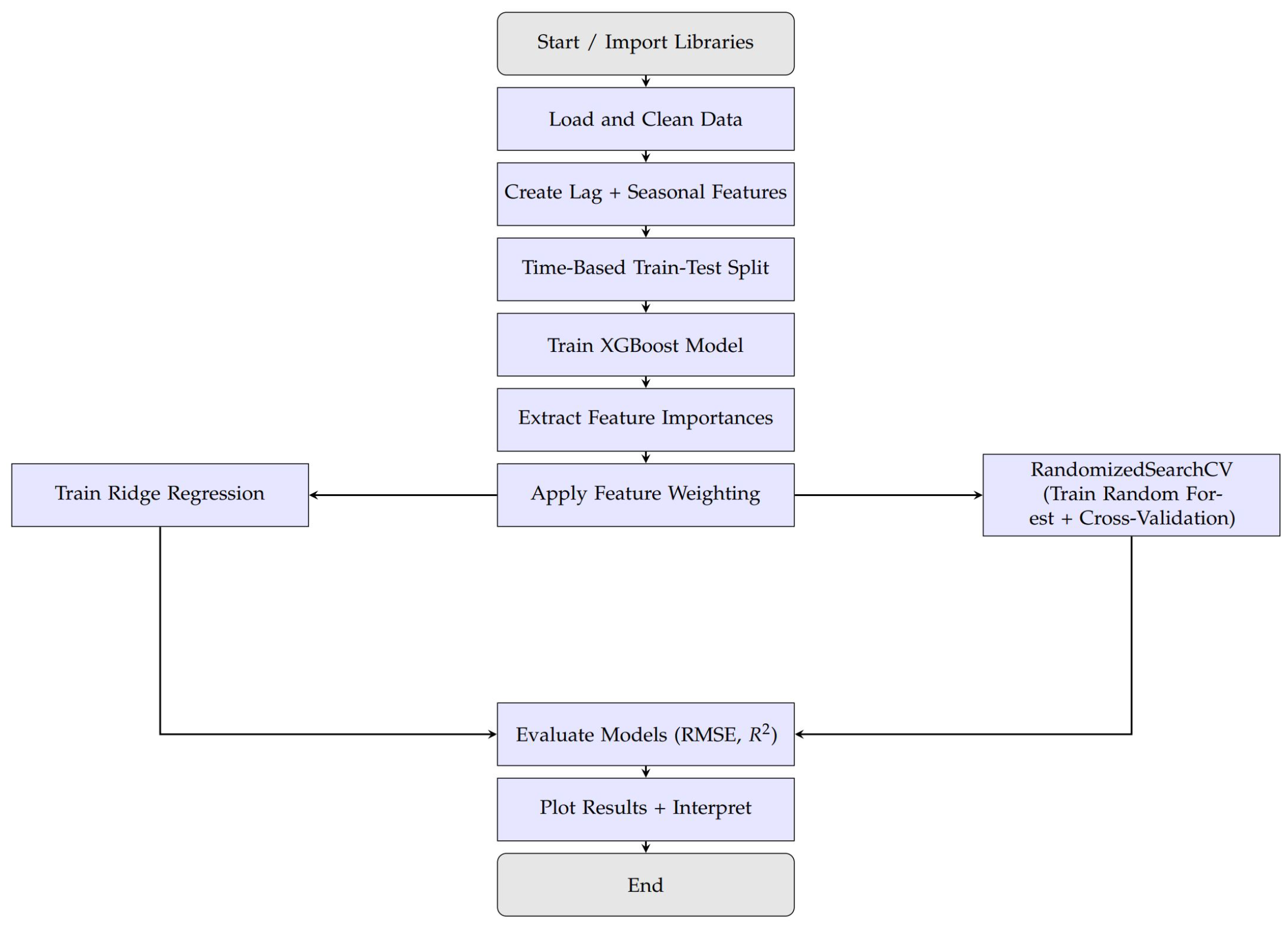
  • To develop an explainable ensemble-based predictive framework for forecasting LWE that incorporates lag features, temporal encodings, and feature re-weighting using XGBoost importance scores.
  • To integrate SHAP for both global and local interpretability, providing transparent insights into the climatic drivers of groundwater storage dynamics.
  • To evaluate and compare the predictive performance of the proposed model against baseline models (Persistence, Standard Ridge Regression, Random Forest, and XGBoost), demonstrating its superiority through statistical metrics (RMSE and R 2 ).
  • To offer a scalable, interpretable, and data-driven forecasting tool that supports sustainable groundwater resource management under conditions of climatic uncertainty and environmental stress.
By bridging the gap between data-driven modeling and actionable insight, this study contributes to the growing body of research on climate-resilient water governance. It demonstrates the potential of explainable machine learning in enhancing our understanding of complex hydrological systems and in supporting informed interventions for ecological restoration and sustainability. Although machine learning has been increasingly applied to hydrological modeling in the Lake Urmia Basin, previous studies primarily focused on surface parameters, lacked predictive frameworks for groundwater storage dynamics. In addition, they largely relied on black-box models without explainability. To address these gaps, this study aims to forecast LWE by integrating GRACE-based satellite observations with climatic variables in an explainable machine learning framework, thereby enhancing transparency and supporting climate-adaptive water management.
To address these gaps, the present study pursues the following objectives: (1) to develop a predictive model for LWE forecasting in the Urmia Lake Basin, (2) to incorporate SHAP-based explainability into the proposed machine learning framework for transparent identification of key climatic drivers, and (3) to establish a robust ensemble learning framework combining feature re-weighting and tree-based modeling for hydrological forecasting purposes.
The remainder of this paper is organized as follows: Section 2 presents a review of relevant literature, focusing on the environmental and hydrological challenges in the Urmia Lake Basin as well as the application of machine learning and explainable AI in similar studies; Section 3 describes the study area, data sources, and preprocessing methods used to construct the dataset; Section 4 outlines the methodological framework, including statistical trend analysis, machine learning model development, feature engineering, and SHAP-based explainability; finally, Section 5 summarizes the main findings, highlights the contributions of this work, and proposes directions for future research and policy implications.

2. Literature Review

Lake Urmia was at one time among the largest hypersaline lakes in the Middle East, but has undergone alarming environmental degradation over the past few decades. Numerous studies have sought to diagnose the causes of this decline by utilizing satellite remote sensing, hydrological modeling, and more recently machine learning methods to analyze temporal changes and provide decision support for sustainable water management. This section synthesizes the extensive body of literature, emphasizing how the present study builds upon and contributes to this growing research domain.

2.1. Remote Sensing and Hydrological Monitoring of Lake Urmia

The use of satellite data, particularly GRACE and GRACE-FO, has been instrumental in tracking Terrestrial Water Storage (TWS) variations in the Lake Urmia Basin (LUB). Zarinmehr et al. [14] employed GRACE data combined with statistical time series models to predict groundwater level declines, highlighting continued depletion through 2024. Similarly, Tourian et al. [15] presented a multi-sensor approach using GRACE, MODIS, and satellite altimetry to estimate that Lake Urmia lost approximately 70% of its surface area over a period of 14 years.
Studies such as [16] have integrated GRACE with water balance modeling to isolate storage changes in the mountain block versus the basin floor, revealing human-induced extraction to be the dominant factor behind lake shrinkage. Saemian et al. [17] evaluated the Urmia Lake Restoration Program (ULRP), observing only temporary improvements driven by artificial inflows and anomalous precipitation as opposed to long-term recovery.
Khorrami et al. [18] used a model-coupled GRACE-based analysis to estimate that 86% of the lake’s volume was lost between 2003 and 2015. They emphasized evapotranspiration and groundwater overuse as primary causes. Similarly, Issazadeh et al. [19] confirmed through GRACE and Google Earth Engine (GEE) that aquifers in northern LUB experienced severe depletion.

2.2. Advancements in Modeling Techniques

In addition to satellite diagnostics, several studies have applied hydrological and machine learning models for predictive insights. Sabzehee [20] demonstrated the use of CNNs to reconstruct missing GRACE data during the satellite transition, finding that this approach outperformed classical approaches and could ensure continuity in hydrological monitoring. Radman et al. [21] employed LSTM and other deep learning models to predict lake surface area changes, finding LSTM to be the most effective.
Chaudhari [22] incorporated land use changes, finding that anthropogenic drivers (e.g., irrigation, dam construction) played a larger role than climate in Lake Urmia’s desiccation. Moghim [23] corroborated this through GRACE–GLDAS integration, revealing strong negative correlations between temperature and water storage.
Hosseini-Moghari et al. [24] quantified that over 50% of basin water loss and up to 90% of groundwater depletion were attributable to human activity, even simulating scenarios where the lake would not have recovered without human intervention. Taheri et al. [25] tracked surface water changes using Landsat imagery and identified precipitation as the most influential factor on surface water area, followed by temperature and vegetation loss.

2.3. Machine Learning Applications in Water Storage Forecasting and Lake Urmia Studies

Recent years have witnessed growing interest in applying Machine Learning (ML) to hydrological forecasting, particularly in data-scarce or highly variable environments such as the Lake Urmia Basin. Several studies have employed ML algorithms to enhance understanding and prediction of various water-related indicators, including lake levels, soil moisture, drought indices, and terrestrial water storage anomalies.
Shiri et al. [26] applied Extreme Learning Machine (ELM) to forecast daily water levels in Lake Urmia, demonstrating superior accuracy and computational efficiency over traditional methods such as Artificial Neural Networks (ANN) and genetic programming. However, their model focused solely on historical lake level data and lacked integration of climatic variables or long-term groundwater storage dynamics.
In another regional study, Asadollah et al. [27] developed a hybrid ensemble model combining Gradient Boosting and Support Vector Regression (GB-SVR) to estimate in situ soil moisture using remote sensing products. While the model achieved high predictive accuracy, its scope was limited to surface soil moisture estimation and did not explore broader hydrological interactions.
Azizi [28] employed ML and GIS to analyze drought impacts and land use changes in Lake Urmia’s catchment. Their work utilized support vector machines and random forests for spatial classification, emphasizing agricultural land degradation. In contrast to their focus on land transformation, our study emphasizes temporal dynamics of groundwater storage and prediction using explainable AI.
Sakizadeh & Milewski [29] investigated future Land Use/Land Cover (LULC) changes in the Lake Urmia Basin using ensemble ML classifiers and CA–ANN models. While their study provided valuable insights into spatial change patterns, it did not incorporate groundwater or hydrological forecasting. By contrast, our work centers on LWE prediction using time series climate data and interpretable ML.
Soltani & Azari [30] developed GMDH, ELM, and ANN models to estimate Terrestrial Water Storage Anomalies (TWSA) using GRACE/GFO data and meteorological inputs. The best-performing model was used to fill missing data; however, interpretability was not addressed. Our work extends this by applying SHAP-based explainability to identify which climate variables most influence groundwater storage. Finally, several recent contributions have explored deep and ensemble ML models for investigating Lake Urmia’s environmental dynamics. For example, Raheli et al. [31] forecasted salinity indicators using DMLP and SVR models with bootstrap uncertainty quantification.
While a range of ML applications have recently emerged in environmental modeling of the Lake Urmia Basin, several important limitations remain. The studies reviewed in this section have demonstrated the potential of ML in predicting water-related parameters such as lake level, precipitation, soil moisture, and salinity. However, these approaches typically suffer from several key gaps: (i) a predominant focus on surface parameters without directly forecasting subsurface groundwater storage indicators such as LWE, (ii) reliance on black-box machine learning models that lack interpretability and fail to elucidate the influence of climatic drivers, (iii) limited integration of GRACE-based hydrological observations with time series climatic predictors, and (iv) absence of explainable AI tools that can transparently quantify the relative contributions of environmental factors.
To address these gaps, the present study develops an explainable machine learning framework for LWE forecasting that combines feature re-weighting via XGBoost, ensemble modeling via Random Forest, and SHAP-based interpretability. This integrated approach not only enhances predictive performance but also enables transparent understanding of the climatic influences driving groundwater storage variability, thereby offering practical value for sustainable water resource management.
While explainable artificial intelligence techniques such as SHAP and LIME have gained popularity for interpreting ML models, their application in hydrological and environmental modeling remains limited and presents several challenges. First, most XAI approaches offer post hoc explanations without influencing model construction, meaning that transparency is not embedded in the model development phase. Second, the explanations are often local, focusing on individual predictions, while global interpretability, that is, understanding overall model behavior across the dataset, remains less emphasized. Third, in complex environmental systems such as groundwater modeling, feature interactions and nonlinearities may lead to misleading or unstable interpretations if not carefully validated. Moreover, many studies utilizing XAI have tended to prioritize model performance metrics (e.g., RMSE, R 2 ) over comprehensive evaluation of the quality and robustness of explanations. To address these limitations, our study integrates feature weighting during model development and applies SHAP-based interpretation both globally and locally, offering a more coherent and actionable understanding of the climatic drivers influencing groundwater variability.
Recent advances in deep learning have significantly enhanced the monitoring of surface water properties from satellite imagery. Hou et al. [32] developed a hybrid recurrent model based on deep learning to map global lake clarity using Landsat OLI images, while Zhou et al. [33] proposed an optical mechanism-based framework for estimating the trophic state of China’s lakes. Although these approaches demonstrate the power of convolutional and recurrent networks for predicting surface optical parameters, they primarily addressed short-term surface variability and did not consider groundwater storage dynamics or model explainability.
In contrast, the present study aims to forecast long-term groundwater storage in the form of the Lake Water Equivalent (LWE) by integrating satellite-derived climatic indicators with hydrological measurements from GRACE and GLDAS. By incorporating feature weighting through XGBoost and applying SHAP-based interpretability, our ensemble learning framework emphasizes both predictive accuracy and transparency. This distinction in target variables, data sources, and methodological focus highlights the novel contribution of our work toward sustainable groundwater resource management under climatic uncertainty.

2.4. Contribution of the Present Study

While prior studies have extensively examined Lake Urmia’s decline using remote sensing, GIS-based analysis, and traditional hydrological modeling, relatively few have integrated advanced machine learning with explainability techniques to forecast hydrological indicators such as LWE. Most existing approaches have focused on either surface water dynamics, land use changes, or water quality parameters, often employing black-box ML models without interpretable outputs. In contrast, this study develops an explainable machine learning framework that integrates GRACE-based LWE data and satellite-derived climatic variables from GLDAS along with engineered time series features to construct an interpretable predictive modeling approach.
Our methodology utilizes a combination of Ridge Regression, Random Forest, and XGBoost models complemented by SHAP analysis, providing both global and local interpretability of climatic drivers. Unlike earlier studies that emphasized short-term lake level prediction or land classification, we treat the LWE as a unified and physically grounded indicator of groundwater storage and lake health. By incorporating lag-based memory features, seasonal encodings, model-driven feature weighting, and comparison against simple baseline models such as persistence forecasting, our framework not only achieves strong predictive performance but also ensures transparency and robustness in understanding climate–hydrology linkages over a 20-year historical period.
Ultimately, this study offers a novel and complementary addition to the existing literature by combining the forecasting power of ensemble learning with the interpretability of explainable AI. This hybrid approach enhances both the methodological rigor and the practical relevance of predictive hydrology in the Lake Urmia Basin, supporting climate-adaptive water policy, transparent stakeholder communication, and sustainable resource management under conditions of climatic uncertainty.

3. Materials and Methods
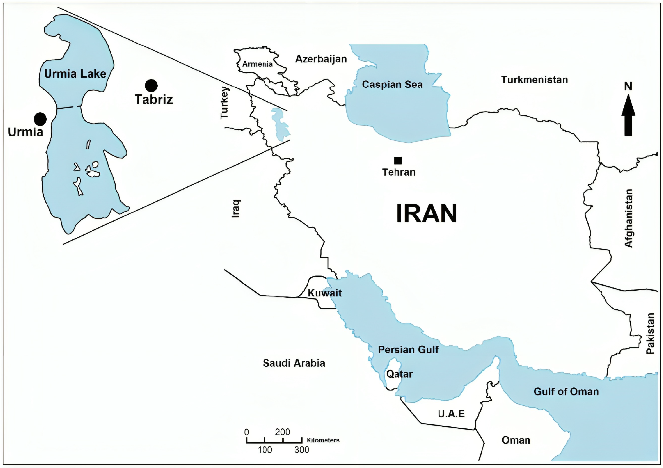
3.1. Case Study

The Urmia Lake basin in northwestern Iran spans 44° 13 to 47° 53 east longitude and 37° to 38° 30 north latitude, covering 51.758 km 2 . As shown in Figure 1, it includes parts of the West Azerbaijan, East Azerbaijan, and Kurdistan provinces [34]. The basin is primarily flat, with altitudes ranging from 1280 to 2000 m above sea level, resulting in a moderate climate with cold winters and mild summers.
The basin receives an average annual precipitation of 320 mm and experiences a mean temperature of 12 °C. These climatic conditions are crucial for the lake’s hydrological cycle and water recharge; however, they have been highly variable due to natural and human-induced factors.
Lake Urmia serves as a vital ecological asset, supporting migratory birds and local agriculture, fishing, and tourism. However, the lake has experienced significant water level decline in recent decades driven by reduced river inflows and increased evaporation due to rising temperatures.
Understanding the geographical and climatic context of the Lake Urmia basin is key to developing sustainable management strategies and addressing the region’s environmental crisis.

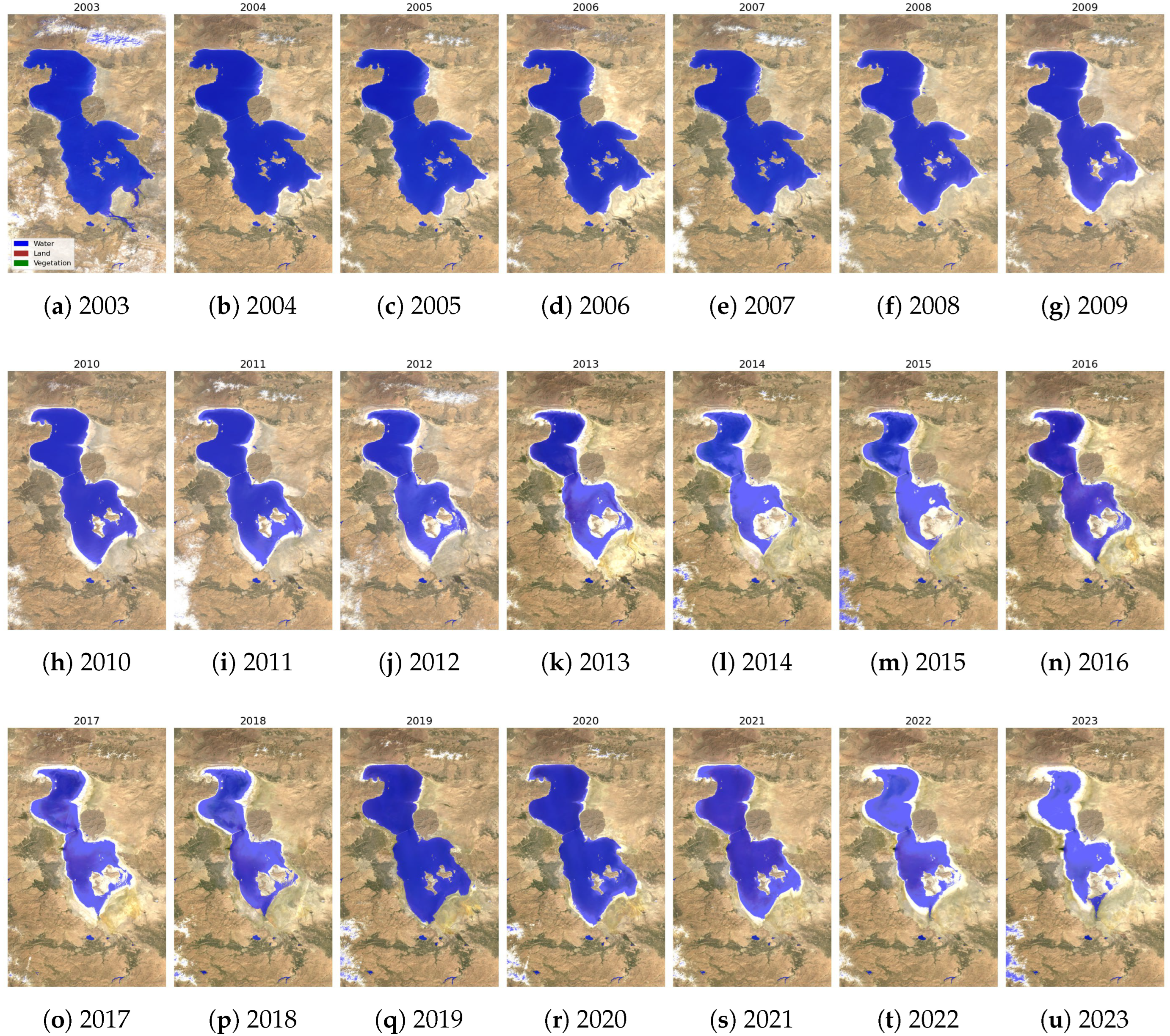
3.2. Changes in Lake Urmia’s Surface Area

Figure 2 presents annual satellite imagery of Lake Urmia, illustrating the lake’s surface area changes over two decades (2003–2023). These images were generated using Google Earth Engine and derived from Landsat satellite datasets. To visualize the spatial extent of surface water in and around Lake Urmia, the NDWI was computed using Landsat 8 imagery. The implementation was carried out in Google Earth Engine, and the corresponding JavaScript code is provided in Appendix A.1. The blue regions represent the water surface, while the surrounding land is depicted in neutral tones. The data source for these images is the United States Geological Survey (USGS), which provides access to Landsat imagery for environmental monitoring. In addition, the raster classification results were visualized using a Python-based Matplotlib script version 3.8.2 in Python 3.11 that allows for custom legends and flexible color rendering. The full code is presented in Appendix A.1.
The early years (2003–2007) depict a relatively stable water surface with minor fluctuations in the lake’s extent, reflecting the lake’s pre-crisis baseline condition. From 2008 onward, a marked decline in the water surface area is visible, coinciding with increased water extraction, reduced inflow from rivers, and prolonged drought conditions. By 2014, significant portions of the lake bed had become exposed, indicating an ecological crisis.
Between 2015 and 2017, the lake experienced severe contraction, with the most dramatic reduction in surface area during this period. By 2017, much of Lake Urmia had dried up, leaving fragmented water bodies. This decline highlights the combined impact of climate change, agricultural water use, and water mismanagement. Signs of post-2018 recovery are evident, likely due to governmental interventions, restoration projects, and favorable climatic conditions. Despite these efforts, the lake’s surface area remains far below historical levels, as shown by fluctuations in water coverage during the final years (2021–2023).
This section focuses solely on presenting the temporal changes in the lake’s surface area as observed through satellite imagery. Detailed analysis and interpretation of these changes, including their drivers and implications, are addressed in subsequent sections.

3.3. Trends of Climatic Variables in the Region (2003–2023)

For temperature, precipitation, soil moisture, and sea level pressure, the dataset includes 20 temporal observations, representing annual averages derived from daily measurements over the 20-year period (2003–2023). For the LWE, the dataset also includes 20 temporal observations, representing yearly averages obtained directly from satellite data (GRACE and GRACE-FO) over the same period.
Figure 3a illustrates the mean annual temperature trends (°C) in the region from 2003 to 2023 based on data from the Iran Meteorological Organization (IMO). Temperatures gradually increased from 2003, peaking around 2009, then exhibited slight fluctuations until 2015. A sharp rise occurred in 2016, reaching the highest recorded temperature in 2017, possibly due to climatic anomalies. Following a notable decline in 2018, temperatures stabilized with modest increases through 2023.
Figure 3b presents the annual precipitation trends (inches) for the same period, again using IMO data. From 2003 to 2009, precipitation showed moderate variability with intermittent peaks, notably in 2008; a gradual decline led to lower levels between 2010 and 2015, followed by a sharp drop in 2016 to the lowest recorded level. Precipitation then increased steeply, peaking in 2019, the highest levels in the timeframe. Levels decreased sharply post-2019, reaching another low in 2022, but showed substantial recovery in 2023.
Figure 3c shows the annual soil moisture trends (%) from 2003 to 2023. Soil moisture data were obtained from the Global Land Data Assimilation System (GLDAS) developed by NASA’s Goddard Space Flight Center. The soil moisture values atre expressed as volumetric water content in percentage (%), representing monthly averages over the study region, and were used to quantify terrestrial water dynamics in the top soil layer. The values indicate a gradual decline in soil moisture from above 26% in the early 2000s to below 24% by 2015. A sharp drop is observed around 2017–2018, with levels falling below 20%, likely reflecting a period of intense drought or anomalous hydrological conditions; however, partial recovery occurs after 2019, with soil moisture rising again toward 24% by 2023. This trend highlights a concerning long-term drying pattern interspersed with short-term recovery phases, aligning with broader climate variability and increasing water stress in the region.
Figure 3d presents annual sea level pressure variations (hPa) over the same period. Pressure declined from 2003 to 2006, reaching its lowest at 25.400 hPa before steadily increasing to a peak above 25.600 hPa around 2010. From 2012 to 2023, pressure remained relatively stable with minor fluctuations except for 2018, concluding with a slight stabilization above 25.500 hPa in 2023. These data were also sourced from the IMO.
Figure 3e illustrates annual variations in LWE thickness from 2003 to 2023, serving as an indicator of water storage changes in the region. Positive LWE values from 2003 to 2005 reflect stable or increasing water storage; however, a consistent decline begins in 2006, with values dropping below zero by 2007 and reaching a significant low of approximately −20 in 2017, likely due to prolonged droughts and increased water withdrawal.
The LWE shows a sharp recovery in 2018, potentially driven by increased precipitation and lower temperatures, as observed in prior figures. After 2018 the values stabilize around zero, indicating possible recovery or equilibrium influenced by policy interventions, reduced water usage, or favorable climatic conditions. This pattern underscores a critical stress period between 2006 and 2017, followed by stabilization after 2018.
The LWE data were retrieved using a JavaScript code developed for Google Earth Engine, incorporating measurements from GRACE (2003–2017) and GRACE-FO (2018–2023) satellites to ensure comprehensive and consistent coverage for the entire study period.

4. Methods

4.1. Statistical Summary of Key Parameters (2003–2023)

Table 1 summarizes key statistics for each parameter using SPSS version 29.0. SPSS was used for its comprehensive statistical capabilities, including normality tests, correlation analysis, and regression modeling, which were integral to this research. Its user-friendly interface and robust tools made it ideal for consistent handling and analysis of the climatic and hydrological datasets utilized in this study.
The mean annual temperature in the study period was 12.32 °C with a standard deviation of 0.58 °C, showing consistent patterns and moderate variability (11.00–13.80 °C). Precipitation averaged 317.86 inches, with higher variability (SD: 76.24 inches) and a range of 157–505 inches, indicating a skewed distribution due to extreme values.
The mean soil moisture was 23.78% (SD: 1.66%), with values ranging from 19.83% to 26.60%, indicating modest inter-annual variability in terrestrial water retention. Sea level pressure was highly stable, with a mean of 25.56 hPa (SD: 0.08 hPa) and a narrow range of 25.36–25.66 hPa. The LWE thickness had a mean of 4.63 inches (SD: 8.68 in), reflecting substantial hydrological variation across years, with values ranging from 20.82 to 5.48  inches.

4.2. Assessment of Normality for Climatic Variables and Groundwater Storage Changes

The normality of the six variables was assessed using Kolmogorov–Smirnov (KS) tests conducted in SPSS software. A p-value greater than 0.05 indicates no significant deviation from normality, permitting the assumption of a normal distribution. Conversely, a p-value less than 0.05 signifies significant deviation, suggesting the need for nonparametric methods or data transformations to address the violation of normality assumptions.
Table 2 presents the results of one-sample Kolmogorov–Smirnov (K–S) tests applied to each variable in the dataset to assess normality. The null hypothesis for this test assumes that the sample data follow a normal distribution. The tested variables included temperature, precipitation, sea level pressure, soil moisture, and LWE, each with 21 valid observations.
The K–S test statistic and corresponding p-values (Asymp. Sig. and Monte Carlo Sig.) indicate that temperature and soil moisture do not significantly deviate from normality at the 0.05 level, with p-values of 0.200 or higher. In contrast, precipitation ( p = 0.069 ), sea level pressure ( p = 0.001 ), and LWE ( p = 0.002 ) significantly deviate from normality, suggesting non-Gaussian distributions.
These results have methodological implications. While temperature and soil moisture can be considered to be approximately normally distributed and suitable for parametric modeling, LWE and sea level pressure may require nonparametric techniques or data transformations to meet statistical assumptions. The use of machine learning models, which are robust to non-normality, helps to mitigate this limitation in the predictive framework. In addition, nonparametric approaches such as the Mann–Whitney U test or Kruskal–Wallis test could be applied. Alternatively, log or other data transformations can be applied to normalize these variables for parametric analyses.

4.3. Spearman Correlation Analysis

Table 3 displays the results of the Spearman’s rank correlation analysis used to examine the monotonic relationships between LWE and four key climate variables: temperature, precipitation, sea level pressure, and soil moisture. This nonparametric test was selected due to the presence of non-normality in several variables (see Table 2).
The strongest significant correlation with LWE was observed for sea level pressure ( ρ = 0.527 , p = 0.014 ), indicating a moderate inverse association in which higher atmospheric pressure tends to coincide with lower LWE values. The strength of association was assessed based on the absolute value of the Spearman correlation coefficient ( | ρ | ) , and statistical significance was determined using a threshold of p < 0.05 , with sea level pressure exhibiting the highest absolute correlation magnitude among the examined variables. Soil moisture also showed a negative but non-significant correlation with LWE ( ρ = 0.155 , p = 0.504 ). Precipitation exhibited a positive but weak correlation with LWE ( ρ = 0.181 ), while temperature had a negative association ( ρ = 0.300 ), though neither of these was statistically significant.
Interestingly, strong inter-variable relationships were also detected. Temperature exhibited a positive correlation with sea level pressure ( ρ = 0.634 , p = 0.002 ), suggesting that higher atmospheric pressure is typically associated with warmer conditions in the region. Soil moisture showed significant negative correlations with both temperature ( ρ = 0.601 , p = 0.004 ) and sea level pressure ( ρ = 0.684 , p < 0.001 ), indicating that elevated temperatures and higher atmospheric pressure tend to reduce soil moisture levels, likely through enhanced evaporation and decreased infiltration. These inter-variable relationships reflect important climatic processes affecting groundwater storage. Higher atmospheric pressure is often associated with stable dry weather conditions, which can lead to increased temperatures and reduced soil moisture. Similarly, higher temperatures accelerate evaporation rates, reducing soil moisture availability. These dependencies highlight that the climate drivers influencing LWE are not independent but rather interconnected, emphasizing the importance of considering multivariate interactions when modeling hydrological responses.

4.4. Analysis of Groundwater Storage Trends

The Mann–Kendall test is a nonparametric method used to detect monotonic trends in time series data without assuming a specific distribution. It is particularly suited for environmental and hydrological applications, helping to identify statistically significant upward or downward trends and estimating the corresponding rate of change (slope).
In this study, the Mann–Kendall test was applied to monthly groundwater storage (LWE) data spanning the period from 2003 to 2023. This period was segmented into two decades (2003–2013 and 2014–2023) in addition to analyzing the entire span (2003–2023). This segmentation strategy was adopted in order to capture potential shifts in groundwater dynamics over time, acknowledging that environmental conditions, policy changes, and climatic drivers might have altered groundwater behavior between the earlier and later decades. Analyzing these sub-periods both separately and jointly provides a more detailed and accurate understanding of temporal groundwater trends. The statistical calculations were performed using a Python script, and the results are summarized in Table 4.
  • 2003–2013: A significant decreasing trend in groundwater storage was detected, with a slope of 0.1721 units per month. The p-value ( p = 0.0000 ) confirms strong statistical significance, and the negative test statistic ( S = 4424.0 ) reflects a consistent decline over this decade.
  • 2014–2023: In contrast, a significant increasing trend emerged in the later decade, with a positive slope of 0.1648 units per month. The p-value ( p = 0.0000 ) indicates strong significance, and the positive test statistic ( S = 2778.0 ) reflects substantial groundwater recovery during this period.
  • 2003–2023: When considering the entire period, a significant decreasing trend was observed, with an overall negative slope of 0.0239 units per month. Although groundwater levels improved after 2014, the earlier substantial decline between 2003 and 2013 outweighed the later recovery, resulting in a net downward trend for the full 21-year period.
These findings highlight the dynamic nature of groundwater fluctuations, where periods of depletion and recovery can coexist within the same region. Segmenting the time series allowed us to detect hidden shifts that only a full-period analysis might have missed. This approach provides a more nuanced understanding of hydrological changes, emphasizing the importance of adaptive water management strategies over different climatic phases.

4.5. Regression and Forecasting Methods

Multiple Regression Analysis

Multiple linear regression analysis was conducted using SPSS software to examine the factors influencing the LWE. This method allows for the identification of relationships between the LWE and multiple independent variables which are considered predictors in this model, such as sea level pressure, precipitation, soil moisture, and temperature. The regression analysis aims to quantify the impact of these predictors on the LWE, helping to identify which factors contribute most significantly to variations in water storage.
Table 5 presents the results of a multiple linear regression analysis aimed at evaluating the combined influence on LWE of key climatic and hydrological predictors, namely, soil moisture (%), precipitation (in), temperature (°C), and sea level pressure (hPa). The model yields a coefficient of determination ( R 2 ) of 0.363 , indicating that approximately 36.3% of the variance in the LWE can be explained by the selected predictors. After adjusting for the number of predictors, the adjusted R 2 drops slightly to 0.204, which still suggests moderate explanatory power given the small sample size. The standard error of the estimate (7.75) reflects the average deviation of the predicted LWE values from the actual observations.
The ANOVA table shows an F-statistic of 2.280 with a corresponding p-value of 0.106, which indicates that the model does not achieve conventional levels of statistical significance (i.e., p < 0.05 ). While the model falls short of being statistically robust, the relatively strong R value (0.603) suggests potential predictive relationships that could be further strengthened with additional data or refined feature engineering. Notably, this model includes soil moisture as a new predictor, improving the R 2 slightly compared to the prior model that omitted it. This highlights the added explanatory value of including surface hydrological variables in LWE modeling efforts.
The standardized regression coefficients (Beta values) reveal that sea level pressure ( β = 0.548 , p = 0.075 ) exerts the strongest negative influence on LWE, followed by soil moisture ( β = 0.256 , p = 0.401 ). Temperature ( β = 0.122 ) and precipitation ( β = 0.222 ) show weaker and statistically non-significant associations. Notably, although none of the individual predictors reach conventional levels of statistical significance (i.e., p < 0.05 ), sea level pressure approaches the threshold and may be an important explanatory variable with a larger sample size.
These findings underscore the multifactorial nature of LWE variability and suggest that pressure and soil moisture are potentially more influential than temperature and precipitation in this context. While the model is not sufficient for precise predictive applications on its own, it serves as a valuable diagnostic tool and baseline for more complex modeling approaches such as ensemble machine learning.
It is important to note that the relatively modest R 2 value is typical for environmental and hydrological studies where multiple unobserved and interacting factors influence the response variable. Although the overall explanatory power is limited, the regression results provide meaningful preliminary insights into the direction and relative importance of climate variables influencing LWE fluctuations.
Moreover, this analysis was included not only to explore direct relationships but also to emphasize the limitations of linear models when dealing with complex environmental systems. The weak performance of the multiple linear regression model highlights the necessity of more advanced forecasting frameworks such as the explainable machine learning models developed later in this study, which are capable of capturing nonlinearities, interactions, and hidden patterns in the data.
The multiple linear regression results suggest that while the model accounts for a moderate portion of the variability in the LWE ( R 2 = 0.363 ), none of the individual predictors (soil moisture, precipitation, temperature, or sea level pressure) are statistically significant at the 0.05 level. This outcome points to several important considerations:
  • Multicollinearity: The presence of correlations among the explanatory variables (as seen in the correlation matrix) may inflate standard errors and obscure the individual effects of predictors, particularly for pressure and soil moisture, which show potential importance.
  • Nonlinearity and Interactions: The assumption of linearity may not adequately capture the complex relationships between hydrometeorological variables and LWE. Interactions or threshold effects could exist, which linear models would fail to detect. The superior performance of nonlinear models such as Random Forest and XGBoost in our study supports this idea.
  • Omitted Variables: Key influencing factors such as groundwater withdrawals, vegetation indices, and human interventions were not included in this model. Their absence may limit the model’s explanatory power and obscure the role of existing variables.
To enhance interpretability and predictive accuracy in future analyses, we recommend: (1) testing for multicollinearity and applying dimensionality reduction techniques (e.g., PCA), (2) considering nonlinear modeling frameworks or interaction terms, and (3) enriching the dataset with additional relevant environmental or anthropogenic indicators. These steps would help to refine the explanatory model and better capture the dynamics governing LWE fluctuations.

4.6. Predictive Modeling Framework Using Ensemble Learning and SHAP-Based Explainability

The proposed framework for LWE prediction integrates advanced machine learning models with post hoc explainability techniques to deliver both predictive accuracy and interpretability. The dataset consists of monthly hydrological and climatic observations from 2003 to 2023. The data were structured for time series modeling after standard preprocessing, including exclusion of irrelevant variables and imputation of missing values through linear interpolation.
To enhance transparency and trust in the modeling outcomes, XAI principles were systematically incorporated. Traditional ML models such as Random Forest and Ridge Regression often act as black-box systems, providing accurate predictions but limited insights into the underlying drivers of model decisions. To address this limitation, we employed SHAP, a robust game-theoretic approach, to decompose the model outputs into additive contributions from each input feature [11].
The SHAP framework facilitates both global interpretability, identifying the most influential predictors across the dataset, and local interpretability, clarifying how individual feature values influence specific predictions. When applied post hoc to the XGBoost surrogate model in our framework, SHAP enabled transparent evaluation of feature impacts. For instance, the SHAP beeswarm plot revealed that higher soil moisture levels positively contributed to LWE predictions, reflecting groundwater recharge processes, while elevated temperatures typically exerted a negative effect, indicating intensified evaporation and water loss.
This integration of SHAP-based interpretability differentiates our framework from traditional ML approaches commonly applied in hydrology, where model evaluation is often confined to performance metrics such as RMSE and R 2 . By offering interpretable and actionable insights into the climatic drivers of groundwater storage dynamics, our framework improves model transparency, strengthens stakeholder trust, and supports evidence-based water management strategies.
To embed temporal memory into the predictive models, lag-based features were engineered, including L W E t 1 , L W E t 2 , and L W E t 3 , along with a rolling mean ( L W E a v g 3 ) and a first-order difference ( L W E d i f f ). Seasonal cyclicity was captured through sine and cosine transformations of the month index, enabling the model to account for annual hydrological variations.
All features were standardized using Z-score normalization. The dataset was split chronologically, reserving the final 24 months as a test set to evaluate model generalization. To guide feature prioritization, the eXtreme Gradient Boosting (XGBoost) algorithm was trained on the standardized training data. XGBoost is a powerful ensemble learning technique that constructs additive decision trees, and has strong predictive performance and robustness against multicollinearity; crucially, it also produces feature importance scores, facilitating informed feature re-weighting and model interpretation.
These scores were used to perform element-wise rescaling of the feature matrix, which is a heuristic approach designed to emphasize the influence of the most predictive variables in subsequent model training. Although the feature importance values were not normalized, their use as re-weighting factors proved beneficial in highlighting signal-rich features. This step was applied consistently to both the Ridge Regression and Random Forest models in order to maintain comparability.
While SHAP values were used afterwards for interpretability, XGBoost was specifically selected for initial feature importance ranking due to its high performance in capturing nonlinear relationships and effective handling of multicollinearity. Unlike SHAP, which provides local interpretability for individual predictions, XGBoost’s built-in feature importance scores offer a straightforward and computationally efficient means of evaluating global feature relevance across the dataset. These importance scores were used to re-weight the input feature space prior to model training, ensuring that the most influential predictors were emphasized during learning. This approach allows for improved model focus on signal-rich features while preserving compatibility with ensemble and regularized models. Additionally, compared to traditional feature selection methods such as mutual information and recursive elimination, XGBoost offers robustness and adaptability in high-dimensional time-dependent hydrological datasets.
Ridge Regression is a regularized linear method. Our model was trained using cross-validation to optimize its penalty term. On the other hand, as Random Forest is an ensemble of decision trees, our model was trained on bootstrap samples and tuned for depth and estimator count. Both models were evaluated on the test set using the Root Mean Squared Error (RMSE) and coefficient of determination ( R 2 ).
Cross-validation techniques were incorporated during model development to ensure robust evaluation and prevent overfitting. Specifically, for Ridge Regression, a 5-fold cross-validation was employed through the RidgeCV function to optimize the regularization penalty parameter ( α ). The training dataset was divided into five subsets; in each iteration, four subsets were used for training and the remaining one for validation, allowing for selection of the most generalizable α value.
For the Random Forest model, although tree-based ensembles are inherently robust against overfitting due to bootstrap aggregation (bagging), hyperparameter tuning was performed using RandomizedSearchCV with 5-fold cross-validation. This approach explored a range of candidate parameters (e.g., number of trees, maximum depth, minimum samples per split) across multiple randomized combinations, ensuring that the best model configuration was selected based on cross-validated R 2 performance. By integrating 5-fold cross-validation for both models during hyperparameter tuning and selection, the proposed framework ensures enhanced generalization, reduced overfitting risk, and improved reliability and interpretability of the LWE forecasts.
Although XGBoost was not used for final prediction, it was retained as a surrogate explainer model for post hoc interpretability using SHAP. SHAP values are based on cooperative game theory, and decompose predictions into additive feature contributions. This enables both global ranking of feature importance and local explanations of individual predictions. The SHAP summary plots confirmed the dominance of recent LWE values and provided meaningful insights into the roles of temperature, precipitation, and soil moisture in influencing lake dynamics.
Figure 4 illustrates the performance and interpretability of the proposed machine learning framework: panel (a) compares actual and predicted LWE values obtained using the Ridge Regression and Random Forest models; panel (b) presents the XGBoost-derived feature importance scores, highlighting the dominance of short-term memory features; and panel (c) shows the SHAP beeswarm plot, providing insight into the directional impact and relative contribution of each feature on model predictions across the test dataset. In addition, the algorithm code outlining the algorithmic structure of the proposed LWE prediction framework is provided, detailing each step from input data preparation and lag-based feature generation to model training, hyperparameter tuning, and SHAP-based interpretability for transparent and data-driven lake water forecasting. Algorithm 1 details the structured steps of the proposed LWE prediction and explainability framework, covering data acquisition, preprocessing, feature engineering (including temporal lags and seasonal encodings), model training with feature re-weighting via XGBoost, SHAP-based interpretability, and visualization of results. Figure 5 complements this by illustrating the overall workflow, providing a visual summary of the sequential process from data preparation to model explainability and interpretation.
Algorithm 1 LWE Prediction and Explainability Framework
  1:
Input: Monthly hydrological and climate dataset from 2003–2023
  2:
Output: Predicted LWE values and SHAP-based feature importance
  Step 1: Data Preparation
  3:
Interpolate missing values using linear interpolation
  4:
Convert and sort dates; set time index
  Step 2: Feature Engineering
  5:
Generate lag features: L W E t 1 , L W E t 2 , L W E t 3
  6:
Create rolling average ( L W E a v g 3 ) and difference ( L W E d i f f )
  7:
Encode seasonality using sin ( month ) , cos ( month )
  Step 3: Feature Scaling and Splitting
  8:
Normalize features using Z-score standardization
  9:
Apply time-based split:
10:
   Train set: all but last 24 months
11:
   Test set: last 24 months
    Step 4: Feature Re-weighting via XGBoost
12:
Train XGBoost on training set
13:
Extract feature importance vector ϕ
14:
Apply feature weighting: X X ϕ
    Step 5: Predictive Modeling
15:
Train Ridge regression (with cross-validation)
16:
Train Random Forest (with tuned hyperparameters)
17:
Predict LWE on test set
18:
Evaluate models using RMSE and R 2
    Step 6: SHAP Explainability
19:
Use trained XGBoost as SHAP explainer model
20:
Compute SHAP values for test samples
21:
Generate SHAP summary plot to assess feature impact
    Step 7: Visualization
22:
Plot actual vs predicted LWE for both models
23:
Visualize SHAP-based feature importance (beeswarm and bar plot)
Figure 4a illustrates the actual versus predicted LWE values over the final 24 months of the dataset, comparing the performance of Ridge Regression and Random Forest models. Both models follow the general trend of the observed LWE, demonstrating their ability to capture seasonal and temporal dynamics. However, notable differences emerge during periods of rapid change. In early 2023, a sharp rise in LWE is observed, followed by a pronounced decline throughout the summer months. The Random Forest model captures these transitions with better fidelity, closely tracking the steep changes. In contrast, the Ridge Regression model lags slightly in responding to these shifts, especially underestimating the recovery period in late 2023. Both models provide similar performance during relatively stable periods such as mid-2022, indicating robustness in non-volatile phases. Overall, Random Forest demonstrates better accuracy and responsiveness, particularly under nonlinear and transitional conditions. This highlights the strength of ensemble tree-based methods in modeling complex environmental dynamics and supports its suitability for operational use in hydrological forecasting.
Figure 4b presents the feature importance scores derived from the XGBoost model, highlighting the relative contribution of each variable to the model’s predictive performance. The first lag of the LWE ( L W E t 1 ) emerges as the most dominant feature, accounting for more than 70% of the total importance. This strong temporal dependency emphasizes the autoregressive nature of LWE dynamics, where recent values significantly inform future states. Secondary features such as L W E d i f f and precipitation ( p r e c i p _ m m ) also contribute meaningfully, reflecting the system’s sensitivity to hydrological inputs and recent directional trends. The inclusion of sinusoidal month encoding ( m o n t h _ s i n ) and temperature ( t e m p _ c e l s i u s ) confirms the seasonal component of lake water variability, although their relative importance remains moderate. Conversely, deeper lag terms ( L W E t 2 , L W E t 3 ), rolling averages, and atmospheric pressure ( p r e s s u r e _ p a ) were found to have minimal influence. These findings suggest that beyond short-term memory, additional temporal lags or static variables offer limited incremental value in this forecasting context. The clear dominance of L W E t 1 justifies its central role in feature weighting and model interpretation.
Figure 4c visualizes the SHAP values for each feature across the test dataset, offering a detailed view of how individual feature values influence LWE predictions. The dominant influence of L W E t 1 is again evident, with high historical values (red points) strongly contributing to increased predicted LWE. This confirms the strong temporal autocorrelation in lake water dynamics. Among the climatic and hydrological features, temperature demonstrates complex behavior; while higher values generally contribute positively, potentially linked to snowmelt contributions, some cases show negative effects, likely due to enhanced evaporation under high heat. Similarly, soil moisture tends to push the LWE predictions upward when elevated, which is consistent with enhanced recharge potential and reduced runoff losses. Precipitation and recent LWE change ( L W E d i f f ) have a balanced distribution of SHAP values, suggesting that their influence is context-dependent, sometimes amplifying LWE when hydrological conditions favor retention while contributing little in other cases. In contrast, features such as the atmospheric pressure and deep lag terms show minimal impact, with SHAP values clustered near zero. This analysis underscores the value of SHAP for transparent model interpretation, allowing for nuanced understanding of how hydroclimatic conditions drive predictive shifts.
Finally, the predictive performance of the proposed framework was evaluated using the Root Mean Squared Error (RMSE) and coefficient of determination ( R 2 ) on the final 24 months of test data. The Ridge Regression model trained on feature-weighted inputs derived from XGBoost importance scores achieved an RMSE of 3.65 and R 2 of 0.86. While this demonstrates solid predictive power, the Random Forest model outperformed it, yielding an RMSE of 3.27 and a higher R 2 of 0.89. This improvement indicates that the ensemble-based Random Forest model better captures the complex nonlinear interactions between features, especially those involving lagged LWE values, temperature, and precipitation. The use of feature weighting based on XGBoost importance contributes to enhanced generalization in both models by emphasizing the most informative predictors. These results validate the robustness of the proposed framework in forecasting lake water volume with high accuracy and explainability.
It is worth mentioning that we applied linear interpolation to address missing values in the satellite-derived and climatic time series data. Linear interpolation is a widely adopted method for hydrological and environmental datasets with relatively small and sporadic gaps [36,37]. In this case, linear interpolation was chosen because it maintains temporal continuity without introducing artificial fluctuations, which is particularly important when modeling long-term groundwater storage trends in order to ensure that autocorrelation structures are preserved for time series feature engineering.
Regarding lag feature selection, lags of one to three months were incorporated for the key climatic variables of precipitation, temperature, soil moisture, and sea level pressure. This decision was based on the recognition of hydrological memory effects and temporal autocorrelation, where changes in climatic conditions impact groundwater storage with a certain delay [38,39]. Preliminary Auto-Correlation Function (ACF) analysis confirmed the relevance of short-term lags. Short-term lags were selected specifically because groundwater systems in semi-arid basins such as the Lake Urmia Basin tend to exhibit rapid responses to climatic forcings (typically within one to three months), reflecting seasonal recharge patterns and limited subsurface buffering capacity. Including lagged variables enhances the model’s ability to capture these delayed climatic influences on LWE, improving predictive performance without introducing unnecessary complexity. This preprocessing step ensured that the feature space maintained both temporal continuity and predictive relevance for downstream ensemble modeling and SHAP-based interpretability.
All codes, processed datasets, and supplementary materials for this study are available from our GitHub repository: https://github.com/habibisara/Urmia-Lake-Climate-Study (accessed on 8 May 2025). Researchers are encouraged to access, test, and build upon this work.

4.7. Performance Comparison Against Baseline Methods

To further validate the effectiveness of the proposed modeling approach, we compared its predictive performance against several baseline methods, including a persistence model, a standard Ridge Regression model without feature weighting, a basic Random Forest model without hyperparameter tuning, and a simple XGBoost model. The results are summarized in Table 6.
The persistence model performed poorly, as expected, with an RMSE of 11.79 and a negative R 2 value, indicating no meaningful predictive capability. While standard machine learning methods such as Ridge Regression without feature weighting (RMSE = 3.91, R 2 = 0.93), Random Forest without cross-validation (RMSE = 3.82, R 2 = 0.89), and XGBoost (RMSE = 3.85, R 2 = 0.90) achieved acceptable results, our proposed Random Forest model with SHAP-based feature weighting and cross-validated hyperparameter tuning outperformed all baselines with an RMSE of 3.31 and an R 2 score of 0.89.
These results clearly demonstrate that incorporating feature importance information and robust cross-validation strategies enhances model accuracy and generalizability for long-term groundwater storage forecasting.    

4.8. Managerial Insights

The results of this study yield several important managerial implications for groundwater resource planning and climate-adaptive policy-making in the Lake Urmia Basin and comparable semi-arid regions.
First, by forecasting the LWE rather than focusing solely on surface parameters, our framework enables a deeper understanding of long-term water availability trends. The target variable is derived from remote sensing data, and reflects subsurface storage variations that are crucial for sustainable basin management.
Second, by integrating multiple climatic predictors such as temperature, precipitation, soil moisture, and sea level pressure, our model captures the complex drivers of groundwater variability. The inclusion of lagged features and seasonal encodings highlights that groundwater responses are not immediate, instead being influenced by accumulated climatic conditions over preceding months. This emphasizes the need for proactive rather than reactive water management strategies.
Third, the use of ensemble learning combined with explainable artificial intelligence techniques, particularly SHAP analysis, enables transparent identification of the most influential factors affecting groundwater storage. For instance, our results show that soil moisture and temperature play significant roles, suggesting that monitoring these variables can provide early warnings of groundwater stress.
Fourth, benchmarking against simple baseline models demonstrates that the feature-weighted ensemble approach significantly improves forecasting accuracy. This enhances the reliability of forecasts for applications such as early drought detection, strategic water allocation, and evaluation of restoration policies.
Overall, the explainable forecasting framework developed in this study empowers environmental planners and decision-makers with a transparent data-driven tool to better understand groundwater dynamics, prioritize monitoring efforts, and design more resilient water management policies in the face of climatic uncertainty.

4.9. Limitations and Future Research Directions

While the proposed framework demonstrates strong predictive performance and valuable explainability, several limitations and avenues for future work remain:
  • Limited Feature Scope: While the current model uses key hydroclimatic variables, it does not yet include land use changes, human interventions (e.g., irrigation or dam operations), or groundwater extraction data, which can significantly impact LWE.
  • Fixed Temporal Resolution: This study is based on monthly aggregates. Exploring models with finer temporal resolution (e.g., weekly or daily) or adaptive time windows could better capture short-term fluctuations and improve responsiveness.
  • Geographic Generalizability: The proposed framework was trained and evaluated only on data for Lake Urmia. Extending the model to other basins or performing transfer learning could test its generalizability and broader applicability.
  • Model Ensemble Optimization: Although Random Forest and Ridge Regression were used, future work could investigate more advanced hybrid or deep learning architectures (e.g., LSTM networks) while preserving interpretability via SHAP or surrogate models.
  • Uncertainty Quantification: The current setup only provides point estimates; integrating probabilistic modeling or Bayesian machine learning could additionally offer confidence intervals and risk-aware forecasting.
  • Physical-Model Fusion: Combining data-driven approaches with physical hydrological models could enhance accuracy and interpretability, especially under unseen extreme conditions.
These directions can help to enhance the robustness, adaptability, and general utility of the proposed LWE prediction and explainability framework, thereby supporting its integration into real-time environmental monitoring systems.

5. Conclusions

This study provides a comprehensive assessment of groundwater storage variability in the Lake Urmia Basin using a combination of satellite-based remote sensing, statistical trend analysis, and machine learning modeling. The Mann–Kendall test identified a significant downward trend in LWE during 2014–2023, confirming a critical period of hydrological stress. However, a modest upward recovery trend over the full 20-year period suggests the partial effectiveness of recent climatic and policy-based interventions.
Correlation and regression analyses highlighted sea level pressure and soil moisture as potential climatic influencers of LWE, although multicollinearity and limited sample size constrained their statistical significance in linear models. This limitation was addressed through the development of a robust machine learning framework leveraging XGBoost for feature prioritization and SHAP for interpretability.
The proposed explainable machine learning framework constitutes a key contribution of this work. By integrating satellite-derived climatic variables, feature re-weighting using XGBoost importance scores, and transparent interpretation through SHAP analysis, the proposed framework achieved high predictive accuracy (Random Forest model: RMSE = 3.27, R 2 = 0.89 ) while maintaining interpretability. The inclusion of lag-based memory features and seasonal encoding further enhanced model responsiveness to hydrological dynamics. Importantly, SHAP analysis revealed the dominant role of short-term LWE memory in influencing lake water predictions, followed by temperature and soil moisture. This dual focus on both predictive performance and explainability differentiates our framework from prior black-box approaches, offering practical insights for climate-adaptive water management.
In addition to the autoregressive effects, several environmental variables were found to influence the LWE dynamics, aligning with physical hydrological processes. Precipitation plays a direct role as the primary input of surface and subsurface water, contributing to positive shifts in lake storage, particularly during wet seasons. Soil moisture, although a more indirect indicator, reflects catchment saturation levels and infiltration potential, both of which influence runoff behavior and eventual lake recharge. Temperature also emerged as a moderately important predictor, as it governs evaporation rates and snowmelt timing, both of which are critical processes in semi-arid basins such as the Lake Urmia watershed. Atmospheric pressure showed minimal direct impact, but reflected broader climatic conditions.
In summary, this study demonstrates that combining remote sensing, feature engineering, ensemble learning, and explainability tools can lead to accurate and transparent groundwater forecasting models. By moving beyond traditional linear approaches, the proposed framework offers a scalable and interpretable solution for supporting sustainable groundwater management in data-scarce and climate-sensitive regions such as the Lake Urmia Basin.
Future research should expand the feature space to include anthropogenic factors, explore finer temporal resolutions, incorporate uncertainty quantification, and investigate hybrid models blending physical and data-driven approaches in order to further enhance predictive reliability and operational applicability.

Author Contributions

Methodology, S.H. and S.T.H.; Software, S.H. and S.T.H.; Validation, S.T.H.; Investigation, S.H. and S.T.H.; Writing—original draft, S.H.; Writing— review & editing, S.T.H.; Visualization, S.H.; Supervision, S.T.H. All authors have read and agreed to the published version of the manuscript.

Funding

This research received no external funding.

Data Availability Statement

All processed datasets and code used in this study are publicly available at: https://github.com/habibisara/Urmia-Lake-Climate-Study (accessed on 8 May 2025).

Conflicts of Interest

The authors declare no conflict of interest.

Appendix A

Appendix A.1. JavaScript Code for Visualizing Water Bodies Around Lake Urmia

Listing A1. JavaScript code for extracting and visualizing water bodies around Lake Urmia using NDWI and Landsat 8 imagery.
Water 17 01431 i001

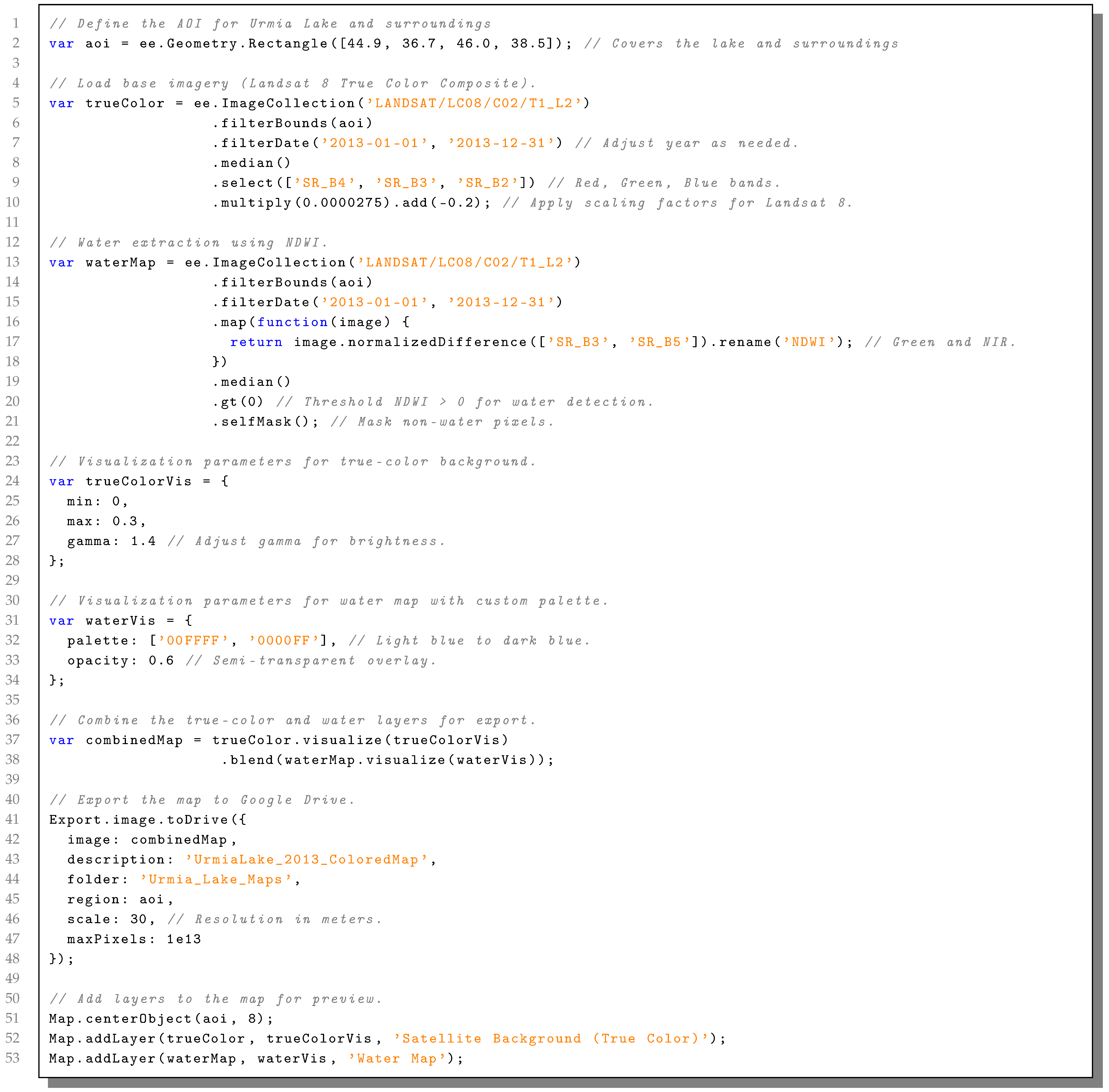
Appendix A.2. Python Script for Visualizing Raster Files

Listing A2. Python script used for visualizing raster data and adding a legend via Matplotlib.
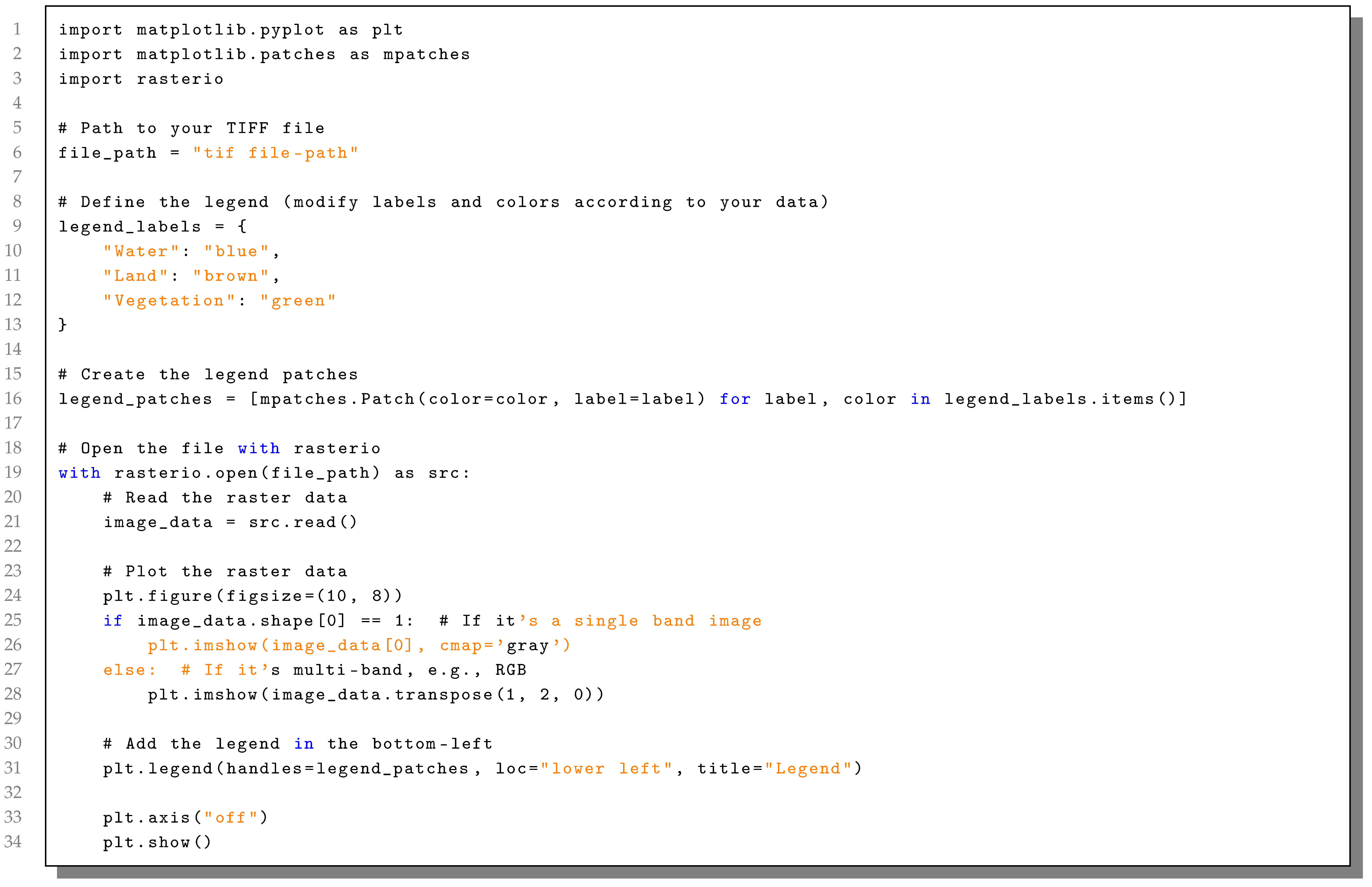
Water 17 01431 i002

References

  1. Ahmadaali, J.; Barani, G.-A.; Qaderi, K.; Hessari, B. Analysis of the effects of water management strategies and climate change on the environmental and agricultural sustainability of Urmia Lake Basin, Iran. Water 2018, 10, 160. [Google Scholar] [CrossRef]
  2. Kazemi Garajeh, M.; Haji, F.; Tohidfar, M.; Sadeqi, A.; Ahmadi, R.; Kariminejad, N. Spatiotemporal monitoring of climate change impacts on water resources using an integrated approach of remote sensing and Google Earth Engine. Sci. Rep. 2024, 14, 5469. [Google Scholar] [CrossRef]
  3. Ghazi, B.; Dutt, S.; Torabi Haghighi, A. Projection of future meteorological droughts in Lake Urmia Basin, Iran. Water 2023, 15, 1558. [Google Scholar] [CrossRef]
  4. Habibi, S. A long-term study of the effects of wastewater on some chemical and physical properties of soil. J. Appl. Res. Water Wastewater 2019, 6, 156–161. [Google Scholar]
  5. Garousi, V.; Najafi, A.; Samadi, A.; Rasouli, K.; Khanaliloo, B. Environmental crisis in Lake Urmia, Iran: A systematic review of causes, negative consequences and possible solutions. In Proceedings of the 6th International Perspective on Water Resources & the Environment (IPWE), Izmir, Turkey, 7–9 January 2013. [Google Scholar]
  6. Ahrari, A.; Sharifi, A.; Haghighi, A.T. Anthropogenic vs. climatic drivers: Dissecting lake desiccation on the Iranian plateau. J. Environ. Manag. 2024, 368, 122103. [Google Scholar] [CrossRef]
  7. Mosavi, A.; Ozturk, P.; Chau, K.-W. Flood prediction using machine learning models: Literature review. Water 2018, 10, 1536. [Google Scholar] [CrossRef]
  8. Sit, M.; Demir, I. A comprehensive review of deep learning applications in hydrology and water resources. J. Hydrol. 2020, 588, 125096. [Google Scholar] [CrossRef]
  9. Reichstein, M.; Camps-Valls, G.; Stevens, B.; Jung, M.; Denzler, J.; Carvalhais, N.; Prabhat, F. Deep learning and process understanding for data-driven Earth system science. Nature 2019, 566, 195–204. [Google Scholar] [CrossRef]
  10. Molnar, C. Interpretable Machine Learning. Leanpub. 2022. Available online: https://christophm.github.io/interpretable-ml-book/ (accessed on 11 April 2025).
  11. Lundberg, S.M.; Lee, S.-I. A unified approach to interpreting model predictions. Adv. Neural Inf. Process. Syst. 2017, 30, 4765–4774. [Google Scholar]
  12. Lundberg, S.M.; Erion, G.G.; Lee, S.-I. From local explanations to global understanding with explainable AI for trees. Nat. Mach. Intell. 2020, 2, 56–67. [Google Scholar] [CrossRef]
  13. Dehghanipour, A.H.; Moshir Panahi, D.; Mousavi, H.; Kalantari, Z.; Tajrishy, M. Effects of Water Level Decline in Lake Urmia, Iran, on Local Climate Conditions. Water 2020, 12, 2153. [Google Scholar] [CrossRef]
  14. Zarinmehr, H.; Tizro, A.T.; Fryar, A.E.; Pour, M.K.; Fasihi, R. Prediction of groundwater level variations based on gravity recovery and climate experiment (GRACE) satellite data and a time-series analysis: A case study in the Lake Urmia Basin, Iran. Environ. Earth Sci. 2022, 81, 180. [Google Scholar] [CrossRef]
  15. Tourian, M.J.; Elmi, O.; Chen, Q.; Devaraju, B.; Roohi, S.; Sneeuw, N. A spaceborne multisensor approach to monitor the desiccation of Lake Urmia in Iran. Remote Sens. Environ. 2015, 156, 349–360. [Google Scholar] [CrossRef]
  16. Aghayi, M.M.; Tajrishy, M.; Guan, H. Assessing mountain block water storage changes in river basins using water balance and GRACE: A case study on Lake Urmia Basin of Iran. J. Hydrol. Reg. Stud. 2023, 49, 101511. [Google Scholar] [CrossRef]
  17. Saemian, P.; Elmi, O.; Vishwakarma, B.D.; Tourian, M.J.; Sneeuw, N. Analyzing the Lake Urmia restoration progress using ground-based and spaceborne observations. Sci. Total Environ. 2020, 739, 139857. [Google Scholar] [CrossRef]
  18. Khorrami, B.; Ali, S.; Sahin, O.G.; Gunduz, O. Model-coupled GRACE-based analysis of hydrological dynamics of drying Lake Urmia and its basin. Hydrol. Process. 2023, 37, e14893. [Google Scholar] [CrossRef]
  19. Issazadeh, V.; Argany, M. Changes in water surface of aquifers using GRACE satellite data in the Google Earth Engine: A study of the Urmia Lake watershed from 2002 to 2017. Town Country Plan. 2021, 13. [Google Scholar] [CrossRef]
  20. Sabzehee, F.; Amiri-Simkooei, A.; Kerachian, R.; Sharifi, M. CNN-based reconstruction of water storage anomaly gaps in Urmia Lake Basin during the GRACE and GRACE-FO transition. Preprint or Unpublished Work.
  21. Radman, A.; Akhoondzadeh, M.; Hosseiny, B. Monitoring and predicting temporal changes of Urmia Lake and its basin using satellite multi-sensor data and deep-learning algorithms. PFG J. Photogramm. Remote Sens. Geoinf. Sci. 2022, 90, 319–335. [Google Scholar] [CrossRef]
  22. Chaudhari, S. Modeling and Remote Sensing of Water Storage Change in Lake Urmia Basin, Iran; Michigan State University: East Lansing, MI, USA, 2017. [Google Scholar]
  23. Moghim, S. Assessment of water storage changes using GRACE and GLDAS. Water Resour. Manag. 2020, 34, 685–697. [Google Scholar] [CrossRef]
  24. Hosseini-Moghari, S.M.; Araghinejad, S.; Tourian, M.J.; Ebrahimi, K.; Döll, P. Quantifying the impacts of human water use and climate variations on recent drying of Lake Urmia basin: The value of different sets of spaceborne and in situ data for calibrating a global hydrological model. Hydrol. Earth Syst. Sci. 2020, 24, 1939–1956. [Google Scholar] [CrossRef]
  25. Taheri Dehkordi, A.; Valadan Zoej, M.J.; Ghasemi, H.; Jafari, M.; Mehran, A. Monitoring long-term spatiotemporal changes in Iran surface waters using Landsat imagery. Remote Sens. 2022, 14, 4491. [Google Scholar] [CrossRef]
  26. Shiri, J.; Shamshirband, S.; Kisi, O.; Karimi, S.; Bateni, S.M.; Hosseini Nezhad, S.H.; Hashemi, A. Prediction of water-level in the Urmia Lake using the extreme learning machine approach. Water Resour. Manag. 2016, 30, 5217–5229. [Google Scholar] [CrossRef]
  27. Asadollah, S.B.H.S.; Sharafati, A.; Saeedi, M.; Shahid, S. Estimation of soil moisture from remote sensing products using an ensemble machine learning model: A case study of Lake Urmia Basin, Iran. Earth Sci. Inform. 2024, 17, 385–400. [Google Scholar] [CrossRef]
  28. Azizi, S. Drought and Environmental Transformations of Lake Urmia: An Integrated Analysis Using Machine Learning and GIS. Eur. J. Appl. Sci. 2024, 12. [Google Scholar] [CrossRef]
  29. Sakizadeh, M.; Milewski, A. Quantifying LULC changes in Urmia Lake Basin using machine learning techniques, intensity analysis and a combined method of cellular automata (CA) and artificial neural networks (ANN)(CA-ANN). Model. Earth Syst. Environ. 2024, 10, 2011–2030. [Google Scholar] [CrossRef]
  30. Soltani, K.; Azari, A. Terrestrial water storage anomaly estimating using machine learning techniques and satellite-based data (a case study of Lake Urmia Basin). Irrig. Drain. 2024, 73, 215–229. [Google Scholar] [CrossRef]
  31. Raheli, B.; Talebbeydokhti, N.; Saadat, S.; Nourani, V. Uncertainty assessment of surface water salinity using standalone, ensemble, and deep machine learning methods: A case study of Lake Urmia. Iran. J. Sci. Technol. Trans. Civ. Eng. 2024, 48, 1029–1047. [Google Scholar] [CrossRef]
  32. Hou, X.; Zhu, Y.; Guo, H.; Yang, D.; Guo, J.; Zhou, Y. Water clarity mapping of global lakes using a novel hybrid deep-learning-based recurrent model with Landsat OLI image. Water Res. 2022, 218, 118536. [Google Scholar]
  33. Zhou, Y.; Hou, X.; Guo, J.; Yang, D.; Zhu, Y.; Guo, H. An optical mechanism-based deep learning approach for deriving water trophic state of China’s lakes from Landsat images. Water Res. 2024, 260, 120301. [Google Scholar]
  34. Choopan, Y.; Emami, S. Optimal operation of dam reservoir using gray wolf optimizer algorithm (case study: Urmia Shaharchay Dam in Iran). J. Soft Comput. Civ. Eng. 2019, 3, 47–61. [Google Scholar]
  35. Asem, A.; Eimanifar, A.; Djamali, M.; De los Rios, P.; Wink, M. Biodiversity of the hypersaline Urmia Lake National Park (NW Iran). Diversity 2014, 6, 102–132. [Google Scholar] [CrossRef]
  36. Li, H.; Sheffield, J.; Wood, E.F. Bias correction of monthly precipitation and temperature fields from Intergovernmental Panel on Climate Change AR4 models using equidistant quantile matching. J. Geophys. Res. Atmos. 2010, 115, D10101. [Google Scholar] [CrossRef]
  37. Schafer, J.L.; Graham, J.W. Missing data: Our view of the state of the art. Psychol. Methods 2002, 7, 147–177. [Google Scholar] [CrossRef] [PubMed]
  38. Nygren, M.; Barthel, R.; Allen, D.M.; Giese, M. Exploring groundwater drought responsiveness in lowland post-glacial environments. Hydrogeol. J. 2022, 30, 1937–1961. [Google Scholar] [CrossRef]
  39. Saqr, A.M.; Kartal, V.; Karakoyun, E.; Abd-Elmaboud, M.E. Improving the accuracy of groundwater level forecasting by coupling ensemble machine learning model and Coronavirus Herd Immunity Optimizer. Water Resour. Manag. 2025; In Press. 1–28. [Google Scholar]
Figure 1. Map of Lake Urmia basin. Adapted from Asem et al. [35].
Water 17 01431 g001
Figure 2. Annual surface area of Lake Urmia extracted from satellite images between 2003 and 2023. Each panel (au) corresponds to the respective year.
Water 17 01431 g002
Figure 3. Variations in climatic and hydrological variables during the study period: (a) temperature, (b) precipitation, (c) soil moisture, (d) sea level pressure, and (e) Lake Water Equivalent (LWE).
Water 17 01431 g003
Figure 4. Model evaluation and explainability visualizations: (a) predicted vs. actual LWE; (b) XGBoost-based feature importance; (c) SHAP-based feature contributions across the test set.
Water 17 01431 g004
Figure 5. Flowchart of the LWE prediction and explainability framework.
Water 17 01431 g005
Table 1. Statistical summary of climatic and hydrological variables in the Lake Urmia Basin (2003–2023).
StatisticsTemperature (°C)Precipitation (in)Sea Level Pressure (hPa)Soil Moisture (%)LWE (in)
Mean12.32005317.8625.5571923.78035 4.63548
Median12.20000309.0025.5881823.89875 0.00100
Std. Deviation0.5808876.2410.078901.656698.68347
Minimum11.00015725.36019.8283 20.824
Maximum13.80050525.65526.60195.483
Table 2. Assessment of normality for climatic variables the Lake Urmia basin.
CategoryStatisticTemperature (°C)Precipitation (in)Sea Level Pressure (hPa)Soil Moisture (%)LWE (in)
Normal Parameters a,bMean12.32005317.8625.5571923.78035 4.63548
Std. Deviation0.5808876.2410.078901.656698.68347
Most Extreme DifferencesAbsolute0.1470.1820.2490.1460.241
Positive0.1240.1820.1160.1060.122
Negative 0.147 0.091 0.249 0.146 0.241
Test Statistic0.1470.1820.2490.1460.241
Asymp. Sig. (2-tailed) c0.200 d0.0690.0010.200 d0.002
Monte Carlo Sig. (2-tailed) eSig.0.2610.0650.0010.2660.002
99% CI Lower Bound0.2490.0590.0000.2550.001
99% CI Upper Bound0.2720.0720.0020.2780.003
Note: a Test distribution is normal. b Calculated from data. c Lilliefors significance correction. d This is a lower bound of the true significance. e Based on 10,000 Monte Carlo samples with starting seed 2,000,000.
Table 3. Spearman correlation analysis results.
VariablesTemperature (°C)Precipitation (in)Sea Level Pressure (hPa)Soil Moisture (%)LWE (in)
Temperature (°C)1.000 0.204 0.634 **−0.601 **−0.300
Sig. (2-tailed) 0.3750.0020.0040.186
Precipitation (in) 0.204 1.000 0.021 0.135 0.181
Sig. (2-tailed)0.375 0.9270.5590.433
Sea Level Pressure (hPa)0.634 ** 0.021 1.000−0.684 **−0.527 *
Sig. (2-tailed)0.0020.927 < 0.001 0.014
Soil Moisture (%)−0.601 ** 0.135 −0.684 **1.0000.155
Sig. (2-tailed)0.0040.559 < 0.001 0.504
LWE (in) 0.300 0.181−0.527 *0.1551.000
Sig. (2-tailed)0.1860.4330.0140.504
  Note: ** Correlation is significant at the 0.01 level (2-tailed). * Correlation is significant at the 0.05 level (2-tailed).
Table 4. Mann–Kendall trend analysis results for monthly groundwater storage (2003–2023).
Parameter2003–20132014–20232003–2023
TrendDecreasingIncreasingDecreasing
Slope−0.17210.1648−0.0239
p-value0.00000.00000.0133
Test Statistic (S)−4424.02778.0−3312.0
Table 5. Regression and residual analysis results.
ModelVariables EnteredVariables RemovedMethod
1Soil Moisture (%),
Precipitation (in),
Temperature (°C),
Sea Level Pressure (hPa)
NoneEnter (All predictors entered together)
Model Summary
ModelRR SquareAdjusted R SquareStd. Error of Estimate
10.6030.3630.2047.748
ANOVA Results
ModelSum of SquaresdfMean SquareFSig.
Regression547.4774136.8692.2800.106
Residual960.5761660.036
Total1508.05220
Coefficients
PredictorBStd. ErrorBetatSig.
(Constant)1583.779811.373-1.9520.069
Temperature (°C)−1.8304.252−0.122−0.4300.673
Precipitation (in)0.0250.0270.2220.9380.362
Sea Level Pressure (hPa)−60.33731.724−0.548−1.9020.075
Soil Moisture (%)−1.3401.554−0.256−0.8620.401
Table 6. Performance comparison of different models.
ModelRMSE R 2 Score
Persistence Model11.79−0.42
Ridge Regression (No Feature Weighting)3.910.93
Random Forest (Simple, No Cross-Validation)3.820.89
XGBoost Model Alone3.850.90
Ridge Regression (Weighted + Cross-Validated)3.650.86
Random Forest (Weighted + Cross-Validated)3.310.89
Disclaimer/Publisher’s Note: The statements, opinions and data contained in all publications are solely those of the individual author(s) and contributor(s) and not of MDPI and/or the editor(s). MDPI and/or the editor(s) disclaim responsibility for any injury to people or property resulting from any ideas, methods, instructions or products referred to in the content.

