Positive–Unlabeled Learning-Based Hybrid Models and Interpretability for Groundwater Potential Mapping in Karst Areas

Abstract

Despite the increasing adoption of machine learning and data-driven models for predicting regional groundwater potential (GWP), exploration geoscientists have recognized that these models still face various challenges in their predictive precision. For instance, the stochastic uncertainty associated with incomplete groundwater investigation inventories and the inherent non-transparency characteristic of machine learning models, which lack transparency regarding how input features influence outcomes, pose significant challenges. This research constructs a bagging-based learning framework that integrates Positive–Unlabeled samples (BPUL), along with ex-post interpretability, to map the GWP of the Lijiang River Basin in China, a renowned karst region. For this purpose, we first aggregated various topographic, hydrological, geological, meteorological, and land conditional factors. The training samples were enhanced with data from the subterranean stream investigated in the study area, in addition to conventional groundwater inventories such as wells, boreholes, and karst springs. We employed the BPUL algorithm with four different base learners—Logistic Regression (LR), k-nearest neighbor (KNN), Random Forest (RF), and Light Gradient Boosting Machine (LightGBM)—and model validation was conducted to map the GWP in karst regions. The findings indicate that all models exhibit satisfactory performance in GWP mapping, with the hybrid ensemble models (RF-BPUL and LightGBM-BPUL) achieving higher validation scores. The model interpretation of the aggregated SHAP values revealed the contribution patterns of various conditional factors to groundwater distribution in karst zones, emphasizing that lithology, the multiresolution index of valley bottom flatness (MRVBF), and the geochemical element calcium oxide (CaO) have the most significant impact on groundwater enrichment in karst zones. These findings offer new approaches and methodologies for the in-depth exploration and scientific prediction of groundwater potential.

1. Introduction

As an essential natural resource for humanity, groundwater plays a crucial role in the sustainable development of ecosystems and society [1,2]. However, owing to exponential population growth, groundwater is being pumped at an unprecedented rate, resulting in deteriorating water quality, rising pumping costs, and land subsidence [3]. Consequently, accurate spatial predictions of groundwater potential areas are essential for developing sustainable strategies for groundwater development, conservation, and management [4,5,6].

Traditional field survey methods, such as hydrogeology, drilling, and geophysical prospecting, are commonly employed to map groundwater potential at small scales [7,8]. While these techniques enable the precise detection of aquifer characteristics, they also have significant drawbacks, including limited coverage, high costs, and slow execution times. This is particularly true for bedrock aquifers, such as karst aquifers, due to their highly heterogeneous aquifer structure [9]. Therefore, the survey and assessment of regional aquifer systems often necessitate the use of remote sensing (RS) and geographic information systems (GIS) to quickly identify and delineate areas of groundwater enrichment, pinpoint key locations, and establish target zones for more detailed exploration efforts.

RS and GIS technologies have the advantages of wide coverage, access to diverse data sources, and flexible methods, making them effective supplements to ground surveys. Spatial multi-source data fusion fundamentally operates through two primary methodologies: the knowledge-driven method and the data-driven method. The knowledge-driven method emphasizes the weighting of criteria (e.g., rainfall, lithology, topography, groundwater level, soil type, land use, slope, flow accumulation, etc.) based on expert judgment to identify areas that are more conducive to groundwater development. Techniques such as the Analytic Hierarchy Process (AHP) [10,11,12], the Technique for Order Preference by Similarity to Ideal Solution (TOPSIS) [13], and the Vlse Kriterijumska Optimizacija Kompromisno Resenje (VIKOR) are employed [14]. Although knowledge-driven methods are straightforward and do not depend on data samples, they are susceptible to behavioral biases in decision-making that can influence expert judgment [15], and may struggle to adapt flexibly to different study areas and groundwater types. Data-driven methods, including statistical models and machine learning techniques, can enhance the accuracy of computational analysis results with nonlinear characteristics through objective mathematical evaluation. Over the past few years, machine learning models have attracted growing interest from researchers. Numerous machine learning methods are employed for groundwater potential mapping, such as Support Vector Machine (SVM) [4], Logistic Regression (LR) [16], k-nearest neighbor (KNN) [17], Artificial Neural Networks (ANNs), the Adaptive Neuro-Fuzzy Inference System (ANFIS) [18], Random Forest (RF) [19,20], Extreme Gradient Boosting (XGBoost), Light Gradient Boosting Machine (LightGBM), and deep learning [21,22]. Previous studies have demonstrated that ensemble learning models—including bagging, boosting, and stacking—which integrate multiple learning algorithms to enhance model performance, are gaining increasing popularity. This trend stems from their higher accuracy compared to traditional machine learning models when generating groundwater potential maps, effectively addressing challenges such as sensitivity to outliers and errors arising from insufficient data [23].

In groundwater potential mapping using machine learning models, the task is typically framed as a binary classification problem, categorizing study areas into “potential zones” (high probability of groundwater occurrence) and “non-potential zones” (low probability). Supervised learning algorithms require both positive samples (locations with confirmed groundwater presence, such as springs, productive wells, or successful boreholes) and negative samples (locations without groundwater, e.g., dry boreholes). However, challenges arise due to the scarcity of readily available negative samples or their limited data volume. When negative samples are not readily available, the common practice is to randomly select locations under specific geographical constraints as substitutes [24,25]. Nonetheless, these “pseudo-negative samples” are obtained from unlabeled areas and may contain areas where groundwater is actually present (e.g., under-explored sites), resulting in label noise, which can greatly increase the uncertainty of the final prediction [26,27]. In contrast, the Positive–Unlabeled learning (PUL) algorithm does not require assumptions about the distribution of negative samples. Instead, it aims to utilize a limited number of positive samples alongside a large amount of unlabeled data during training to develop classifiers with competitive predictive performance [28]. In the actual case of groundwater investigations, it is easier for us to access groundwater points and unknown areas from geospatial space. Therefore, groundwater potential mapping is more accurately equated to the PUL problem. Among the various PUL algorithms, the bagging-based PUL (BPUL) approach can significantly enhance both robustness and discriminatory capability by using bootstrap aggregation techniques. Therefore, integrating various machine learning algorithms with BPUL presents a promising strategy for constructing classification prediction models that are suitable for multiple data sources. This method has been successfully applied in mineral prospect prediction and landslide susceptibility assessment, demonstrating considerable potential [29,30,31]. This investigation centers on constructing BPUL algorithms based on various ensemble learning methods and evaluating their effectiveness in mapping groundwater potential in karst areas. Complex nonlinear transformations in machine learning require additional models to check the results in a human-understandable form during the interpretation process, improving their credibility by employing expert knowledge. Considering the complex hydrogeological processes in karst regions, different models may employ distinct decision-making mechanisms relevant to the study area. Consequently, this study provides a discussion on the decision-making mechanisms within the models, thereby enhancing the transparency of the modelling process.

2. Study Area and Data

2.1. Study Area

The study area, the Lijiang River Basin, is located northeast of the Guangxi Zhuang Autonomous Region, China. It is a world-renowned natural tourism destination and an important ecological economic zone in the country. The basin is situated in the upper reaches of the Guijiang River, a tributary of the Xijiang River system in the Pearl River basin. Geographically, it lies between 24°18′ and 25°41′ north latitude and 109°45′ and 110°40′ east longitude, encompassing a total drainage area of 5815.91 km² (Figure 1). Many studies have demonstrated that the karst geological environment of limestone strata from the Devonian and Carboniferous periods in the Mesozoic era, as well as the fault structures that intersect them, are the dominant controlling factors for the geomorphological features of the Lijiang River Basin today [32,33,34]. The perimeter of the Lijiang River Basin is encircled by low-to-medium mountains and hills, while the central region is predominantly marked by karst landforms, with the Lijiang River Valley traversing the entire area from north to south. In regions where karst development is prominent, a network of various underground cave systems interconnects, creating favorable conditions for the formation and storage of karst groundwater. The basin is situated within a classic East Asian subtropical monsoonal humidity regime, featuring hot and rainy summers alongside cold and humid winters. Rainfall varies significantly with the season; the rainy season, which spans from April to August, constitutes 65% of the annual precipitation; conversely, the dry season, from December to March of the following year, contributes approximately 15% of the yearly total. Maximum precipitation occurs from May to June, gradually decreasing after September, with only localized showers thereafter.

2.2. Samples

Through field surveys, 228 groundwater samples were collected in the study area, comprising 180 observation wells or boreholes and 48 karst springs. All samples were accurately located using handheld GPS during the field investigation (Figure 1). Additionally, multiple subterranean stream systems were investigated within the delineated area, and their approximate flow paths were mapped through geophysical surveys and groundwater tracer tests. To enhance the number of samples for learning, we sampled at 300-m intervals along the subterranean stream flow path, which resulted in an additional 118 groundwater samples (Figure 2). Ultimately, a total of 356 groundwater points, identified as capable of providing groundwater and productive, serve as positive samples for this study. All samples were randomly assigned as training and testing samples in a 7:3 ratio [35].

Except for the positive samples, samples selected from a uniformly spaced 30 m × 30 m grid throughout the study area were utilized as the unlabeled sample set for input to the model.

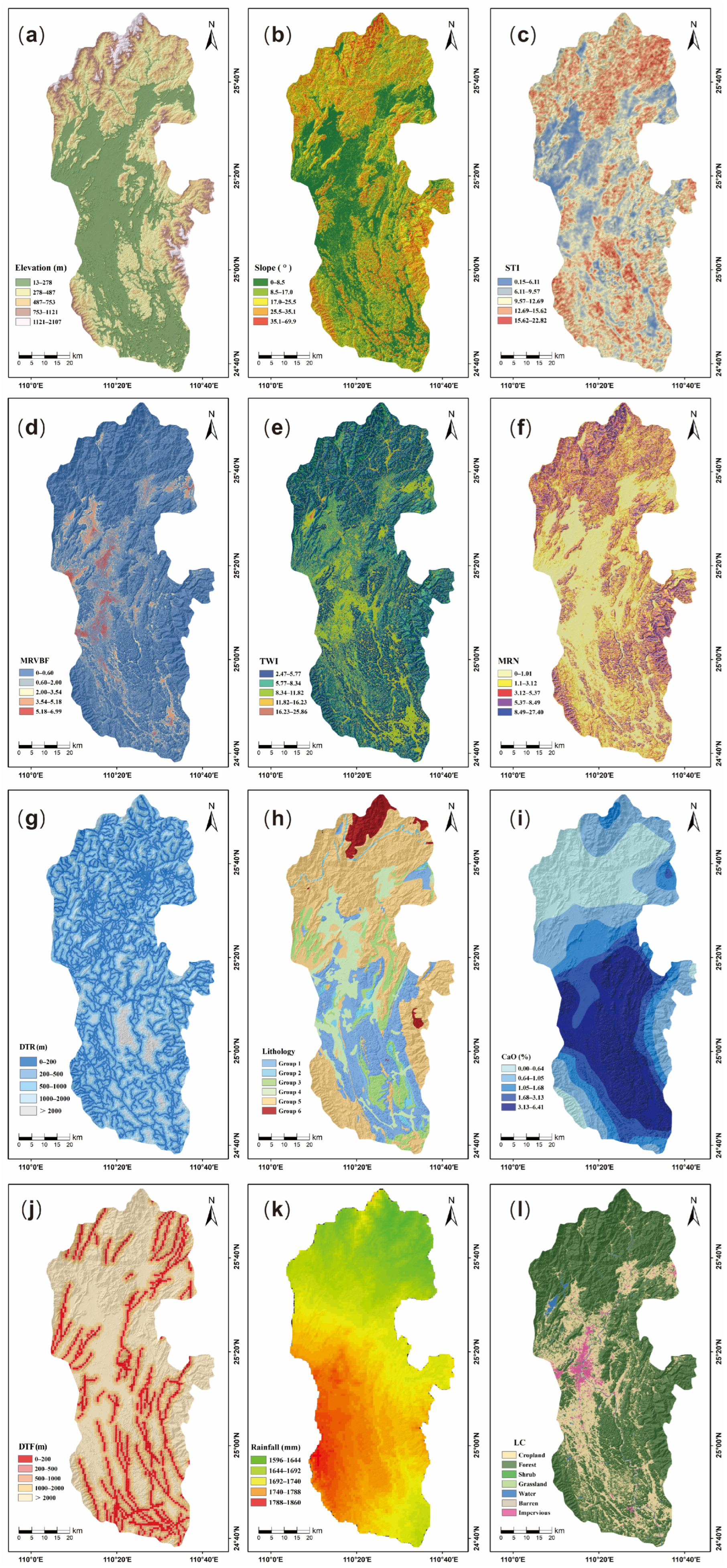
2.3. Groundwater Conditional Factors

Groundwater occurrence is shaped by a range of factors, such as geology, topography, hydrological conditions, and climate change. The precise identification of key determinants influencing groundwater potential zonation and the systematic development of corresponding geospatial thematic layers, through comprehensive consideration of the study area’s prevailing environmental conditions and regional hydrogeological characteristics, constitute critical prerequisites for enhancing the predictive accuracy of hydrogeological assessment models. We reviewed previous studies on predicting groundwater potential [5,6,36,37,38] and collected a comprehensive set of factors that may influence groundwater potential, including topography, hydrology, geology, meteorology, and land cover. Information on datasets related to groundwater conditioning factors can be found in

Table 1. Information on groundwater conditional factors.

Conditional Factors	Data Layers	Database Name	Data Source
Topographical factors	Elevation, slope, STI, MRVBF	ASTER-digital elevation model (spatial resolution 30 m)	https://search.earthdata.nasa.gov (accessed on 12 September 2024)
Hydrological factors	TWI, MRN	ASTER-digital elevation model (spatial resolution 30 m)	https://search.earthdata.nasa.gov (accessed on 12 September 2024)
	DTR	National 1:250,000 Basic Geographic Database	https://www.webmap.cn (accessed on 10 October 2024)
Geological factors	Lithology, DTF	National 1:200,000 Geological Map	http://www.ngac.org.cn (accessed on 10 October 2024)
	CaO	Geochemical Series Maps of China’s Terrestrial Land Area (1:2,500,000)	https://geocloud.cgs.gov.cn (accessed on 10 October 2024)
Meteorological factor	Rainfall	WorldClim 2 (spatial resolution 1 km)	https://worldclim.org (accessed on 12 October 2024)
Land cover factor	LC	The 30 m annual land cover dataset and its dynamics in China from 1990 to 2019	https://doi.org/10.5281/zenodo.4417810 (accessed on 12 October 2024)

. Given that most data utilized in this study have a 30 m resolution, the spatial dataset was projected, transformed, and resampled to a 30 × 30 m² grid. This process ensured that all input layers shared uniform projection and spatial resolution (Figure 3).

2.3.1. Topographical Factors

Topographical factors incorporate five DEM-derived metrics: elevation, slope, surface texture index (STI), and multiresolution index of valley bottom flatness (MRVBF). Elevation is a fundamental topographic factor that governs the flow pathways of surface water, thereby impacting groundwater levels. The slope also serves as a critical hydrogeomorphological factor. Generally, the rate of surface runoff and water infiltration increases with slope steepness [39]. The STI is a morphometric index that quantifies the topographic surface texture by analyzing the spatial distribution of peaks and pits [40]. The MRVBF index effectively identifies flat and low topographical features indicative of valley bottoms across multiple scales. It offers an understanding of the flatness and minimal relief characteristics of valley bottoms, which serve as essential hydrological buffers and significantly influence runoff dynamics [41]. Smaller values suggest erosional terrains where the presence of groundwater aquifers is less probable, whereas values exceeding 1 indicate depositional areas with a higher likelihood of productive groundwater aquifers [42].

2.3.2. Hydrological Factors

This study considers three hydrological factors: the Topographic Wetness Index (TWI), the Melton Ruggedness Number (MRN), and the Distance to Rivers (DTR). The TWI is widely used in groundwater potential assessments, clarifying the relationship between catchment area, slope, and hydrological processes [43]. It is essential in analyzing the impact of topography on groundwater infiltration [44,45]. The MRN is computed as the extremal elevation differentials of a watershed, normalized by its area, and serves as a flow accumulation index [46]. The DTR measures the proximity of any point within the study area to the nearest river, which is a fundamental parameter in hydrological analysis. It influences the ease with which the river recharges the groundwater and also affects the moisture content of the soil and rock on adjacent slopes, thereby impacting the occurrence of groundwater [47].

2.3.3. Geological Factors

Three geological factors—lithology, the geochemical element calcium oxide (CaO), and the Distance to Faults (DTF)—play significant roles in groundwater dynamics. Lithology serves as the medium through which groundwater flows and is stored [48], significantly influencing regional groundwater reserves and their chemical composition [49]. The enrichment characteristics of karst groundwater are closely tied to the type and distribution of soluble rocks, primarily carbonates in this context. Based on the standard 1:200,000 scale geological map covering our research region, we categorized the stratigraphic rock groups within the Lijiang River Basin according to carbonate and non-carbonate rock types. This classification is crucial for understanding the influence of karst-related factors on groundwater potential in an area dominated by karst processes. The results of this categorization are presented in

Table 2. Classification and distribution of carbonate rocks in the study area.

Category Number	Carbonate Rock Type	Stratigraphic Unit	Area Proportion
Group1	Pure carbonates	Tangjiawan, Rongxian, Baqi, Guilin, Yaoyunling	22.20%
Group2	Subpure carbonates	Baidong, Huangjin, E’toucun	2.92%
Group3	Impure carbonates	Donggangling, Liujiang, Yingtang, Wuzhishan, Baping	9.20%
Group4	Covering carbonates	Guiping, Wanggao, Baisha, Lingui	11.90%
Group5	Clasolites	Bianxi, Huang’ai, Xindu, Qingxi, Doushantuo, Laobao, Fulu, Lijiapo, Chang’an, Gongdong, Lianhuashan, Shengping, Tianlinkou, Luzhai, Chuanbutou, Hexian, Luofu, Yongning, Folong’ao	49.76%
Group6	Magmatites	\	4.02%

. Rocks with higher concentrations of Ca²⁺ ions during karstification are more susceptible to dissolution by water, leading to more pronounced and intense karst development in these areas [50,51]. Fractures resulting from tectonic activity function as critical pathways that control groundwater infiltration and are essential for the storage and transport of groundwater, particularly in karst environments [52,53]. The nearer the proximity to a fault and the greater the fracture density, the higher the likelihood of groundwater presence.

2.3.4. Meteorological Factor

The amount of precipitation determines the volume of water that infiltrates the groundwater system, serving as the primary source of recharge [54]. Therefore, historical rainfall data from the past 30 years (1970–2000) [55] were used to compile a map of the average annual rainfall in the Lijiang River Basin.

2.3.5. Land Cover Factor

Land cover types also affect water infiltration and surface runoff. Thus, they are critical for groundwater occurrence and recharge [36,56]. In this study, a map depicting the land cover types in the study area (Figure 3l) was created using global land cover data [57], including categories such as cropland, forest, grassland, shrubland, water, and impervious surfaces.

3. Methodology

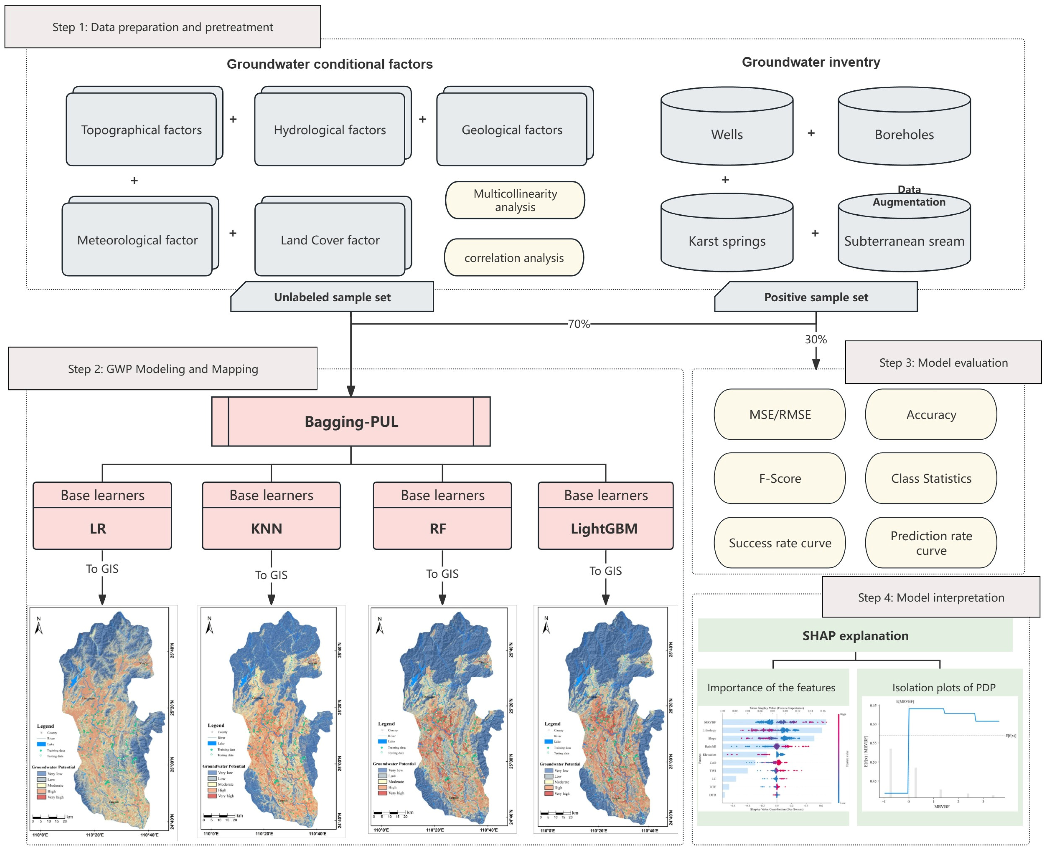
3.1. Research Framework

This research adopts a four-stage methodological framework, as detailed in Figure 4 and the following text: (1) Data preparation and preprocessing, which includes compiling groundwater inventory maps and identifying groundwater potential prediction factors. Multiple collinearity analysis and Spearman correlation analysis were conducted to assess the correlation of factors, thereby eliminating irrelevant or redundant factors. (2) GWP modelling and mapping. Several machine learning classifiers (LR, KNN, RF, LightGBM) were used as base classifiers for hybrid models to train the nonlinear relationships between groundwater samples and their conditional factors. The resulting outputs were imported into ArcGIS 10.6 to create regional groundwater potential prediction maps. (3) Model evaluation. The comparative analysis of prediction accuracy across the four candidate models was conducted using multiple error metrics. (4) Model interpretation. The Shapley additive explanations (SHAP) approach was applied to assess the influence of groundwater conditional factors on groundwater potential in karst areas. The code in this study was implemented in Python 3.10, utilizing Python packages such as scikit-learn1.2.1, lightgbm 4.6.0, and shap0.46.0. The execution was performed on a Windows virtual machine equipped with a 32-core Intel 2.9 GHz processor and 32 GB RAM. Mapping tasks were carried out using ArcGIS 10.6.

3.2. Multicollinearity and Correlation Analysis

Based on a literature review and hydrogeological mechanism analysis, 12 groundwater condition factors were preliminarily selected as predictive variables to evaluate groundwater enrichment levels. To address potential redundancy among variables, Spearman’s correlation analysis was employed to identify redundant factors by calculating the rank correlation coefficient. High-correlation factors with lower contribution were prioritized for elimination according to the threshold of |ρ| > 0.7. In addition, when two or more predictive variables are correlated, the standard error of the coefficients increases, a phenomenon known as multicollinearity [58]. By analyzing the presence of multicollinearity in the model and removing factors with high multicollinearity, we aim to minimize model bias and optimize prediction outcomes. The multicollinearity among groundwater condition factors was quantitatively assessed through variance inflation factor (VIF) and tolerance (TOL) calculations, with the iterative elimination of variables exceeding empirically established thresholds (e.g., VIF > 5, TOL < 0.2).

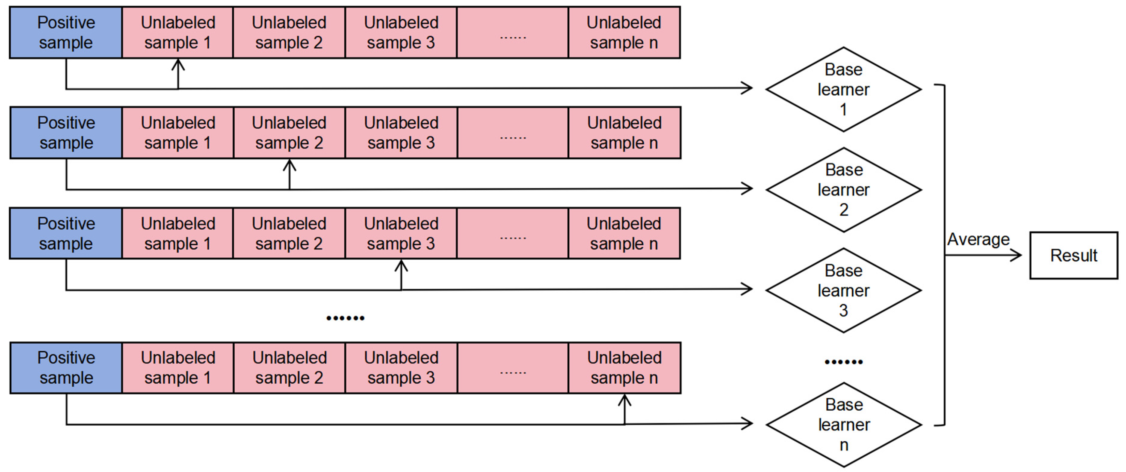
3.3. Bagging Positive–Unlabeled Learning Algorithms

Positive–Unlabeled learning (PUL) is a semi-supervised, single-class classification algorithm that can train a classifier using positive and unlabeled samples. However, when positive samples are insufficient and the ratio of unlabeled data is small, the performance of forward unlabeled learning can fluctuate significantly. In such cases, the bagging strategy proves to be beneficial. Bagging in Positive–Unlabeled learning involves learning a function (h: Y→R) from the positive sample set P and the unlabeled sample set U, which predicts the probability of instances in Y being classified as positive. The process begins by randomly selecting k unlabeled samples from U to create Ut. Then, each subset Ut is combined with P to form a training set, where a base classifier is trained to differentiate between P and Ut. Since the subsets from U are chosen randomly, the empirical pollution varies. After a predefined number of iterations, N, all the scores for each sample are recorded. In the end, N base classifiers are combined to produce the final result, with each sample in U receiving a final score S(x), which is the average of the calculated scores.

$$S(x)={\displaystyle \frac{1}{N}}{\displaystyle \sum _{i=1}^N{f}_t(x)},i=1,2,\cdot \cdot \cdot N$$

(1)

In the bagging-based Positive–Unlabeled learning (BPUL) framework, multiple independently trained base learners with identical distributions are implemented using the previously described procedure (Figure 5). The methodology capitalizes on a limited number of positive examples and employs bootstrap aggregation techniques, which markedly improve the performance and stability of the classification [30,31,59]. It considers all provided positive instances as true positives (TPs) and iteratively subsamples unlabeled instances of equivalent size, ensuring that only a small portion of the unlabeled set U is classified as negative (N) in each iteration, thereby effectively reducing the rate of false-negative errors. BPUL permits the integration of a wide range of supervised machine learning algorithms as its base learners. In this study, the Logistic Regression (LR), k-nearest neighbor (KNN), Random Forest (RF), and Light Gradient Boosting Machine (LightGBM) algorithms were chosen as base learners for BPUL to evaluate their performance differences in groundwater potential mapping. These four models were chosen because they represent distinct algorithmic categories—linear models (LR), instance-based learning (KNN), decision tree ensembles (RF), and gradient boosting machines (LightGBM)—and all of them have demonstrated reliable performance in groundwater potential mapping and related scenarios [21,60,61,62].

3.4. Evaluation Indexes and Model Comparison Method

In light of the absence of reliable negative samples for training and testing purposes, we utilized four prominent metrics to evaluate and compare the accuracy of the established integrated machine learning models: Mean Square Error (MSE), Root Mean Square Error (RMSE), accuracy, and F-score. The corresponding formulas and meanings of these metrics are detailed in

Table 3. Calculation method of evaluation indicators.

Evaluation Index		Formula	Optimum Value	Meaning
Name	Abbreviation
Mean Square Error	MSE	$MSE={\displaystyle \frac{{\displaystyle \sum _{i=1}^n{(y_i-{\widehat{y}}_i)}^2}}{n}}$	0	The mean square of the difference between predicted and true values.
Root Mean Square Error	RMSE	$RMSE=\sqrt{{\displaystyle \frac{{\displaystyle \sum _{i=1}^n{(y_i-{\widehat{y}}_i)}^2}}{n}}}$	0	The root mean square of the difference between predicted and true values.
Accuracy	A	$A={\displaystyle \frac{TP+TN}{TP+FP+TN+FN}}$	1	The proportion of correctly predicted samples (including positive and negative samples) among all samples.
F-Score	F	$F=2\times {\displaystyle \frac{P\times R}{P+R}}$	1	A weighted average of recall and accuracy.

. Accuracy and F-score assess classification performance, while MSE and RMSE quantify the discrepancy between predicted probabilities and actual labels.

Moreover, plotting the success rate curve (SRC) facilitates the evaluation of the classification accuracy for the resulting map of existing groundwater potential areas. The SRC was generated by aligning the training dataset with the groundwater potential map. The prediction rate curve (PRC) indicates the model’s capacity to predict unknown groundwater potential. By comparing the validation dataset to the groundwater potential map, we derived the PRC. The magnitude of the evaluation results was quantitatively assessed by calculating the area under the curve (AUC).

3.5. Zoning Methods of the Groundwater Potential Maps

In zoning groundwater potential maps, common objective methods to avoid subjective classification bias include the quantile method, the natural breaks method, and the equal interval method. Among these, the quantile method divides the classes based on equal amounts of data; however, it may result in the mixing of low- and high-probability values within the same class (e.g., values between 0.2 and 0.8 belonging to the same class), leading to potentially misleading maps. The natural breaks method determines classification boundaries by calculating intra-class homogeneity and inter-class heterogeneity. However, this method relies on data-specific classifications and is not suitable for comparing multiple maps constructed using different underlying information. In contrast, the equal interval method evenly divides the value domain into fixed intervals (e.g., 0.2 for each class), which aligns with the mathematical nature of probability scoring and facilitates the comparison of results from different models [63]. Based on this approach, and in accordance with the common practice of classifying groundwater potential into five categories, as established by previous researchers [64,65], the equal interval method was employed to categorize the scores into five classes: very low [0–0.2], low [0.2–0.4], medium [0.4–0.6], high [0.6–0.8], and very high [0.8–1].

3.6. The Shapley Additive Explanations (SHAP) Approach

Shapley additive explanations (SHAP) is introduced as a representative model-independent interpretability method, inspired by cooperative game theory. In this study, it was applied to the interpretability of four hybrid machine learning models to reveal the internal decision-making mechanisms of the models. This method achieves the post hoc explanation of the decision-making mechanism of machine learning models by quantifying the marginal contribution of each feature to the model’s prediction results. Specifically, SHAP regards each feature as a “player” in the game and the model’s predicted value as the “payoff” of multi-party cooperation. It calculates the weighted average of the contributions of features in all possible subsets. For each prediction sample, the model first generates a predicted value, and then the SHAP value is calculated to represent the contribution of each feature in this sample to the predicted value [66,67]. This approach allows for the interpretation of a “black-box model” at both global and local levels [68]. That is, we not only understand the overall behavior of the entire model, but also gain insights into how the prediction results of specific samples are formed by the joint action of various features. The SHAP value can be expressed as follows:

$${\varphi }_j={\displaystyle \sum _{S\subseteq \left\{x_1,\dots ,x_p\right\}\left\{x_j\right\}}\frac{\left|S\right|!(M-\left|S\right|-1)!}{M!}\left[f(S\cup \left\{x_j\right\})-f(S)\right]}$$

(2)

where ${\varphi }_j$ denotes the contribution of the j-th feature within a specific groundwater sample, i.e., the corresponding SHAP value. M represents the total number of input features, and $x_j$ represents the j-th input feature. S is a subset of the input features, $\left|S\right|$ is a subset of all the features used in the model, and $f(S)$ represents the predicted value of the sample vector x in S.

The output for individual sample features can be defined as follows:

$$g(x^{\prime })={\phi }_0+{\displaystyle \sum _M^{j=1}{\phi }_j}$$

(3)

In this equation, $g(x^{\prime })$ represents the model’s output value, and ${\phi }_0$ refers to the interpretive constant—specifically, the average prediction across all training samples. ${\phi }_j$ denotes the SHAP value for each feature.

In this study, this approach was applied to evaluate the interpretability of four hybrid machine learning models to reveal the internal decision-making mechanisms of the models.

4. Results

4.1. Correlation Between Groundwater Conditional Factors

Figure 6 displays the Spearman correlation matrix analysis of all selected initial conditional factors, revealing that the inter-factor correlations are negligible. We also employed VIF and TOL to assess the presence of multicollinearity across all considered factors. Our analysis indicated that the factors elevation, slope, STI, TWI, and MRN exhibited multicollinearity (TOL < 0.2, VIF > 5). Among the topographic factors, variations in slope and elevation generally led to more significant surface irregularities; therefore, we excluded STI and retained elevation and slope, as simpler factors are easier to interpret in the model. TWI and MRN are both hydrological factors, and we eliminated MRN due to its higher VIF values. Subsequently, we re-conducted the multicollinearity analysis on the remaining ten factors. The findings from the second test reveal no multicollinearity issues among the other conditional factors (

Table 4. Multicollinearity analysis of the conditional factors.

Factor	Original Factor		New Factor
	TOL	VIF	TOL	VIF
Elevation	0.180	5.546	0.200	4.988
Slope	0.112	8.924	0.211	4.748
STI	0.140	7.164	/	/
MRVBF	0.454	2.205	0.537	1.863
TWI	1.000	1.000	1.000	1.000
MRN	0.179	5.597	/	/
DTR	0.476	2.103	0.476	2.102
Lithology	0.867	1.153	0.867	1.153
CaO	0.506	1.976	0.506	1.976
DTF	0.562	1.779	0.562	1.779
Rafall	0.957	1.045	0.958	1.043
LC	0.565	1.770	0.565	1.770

).

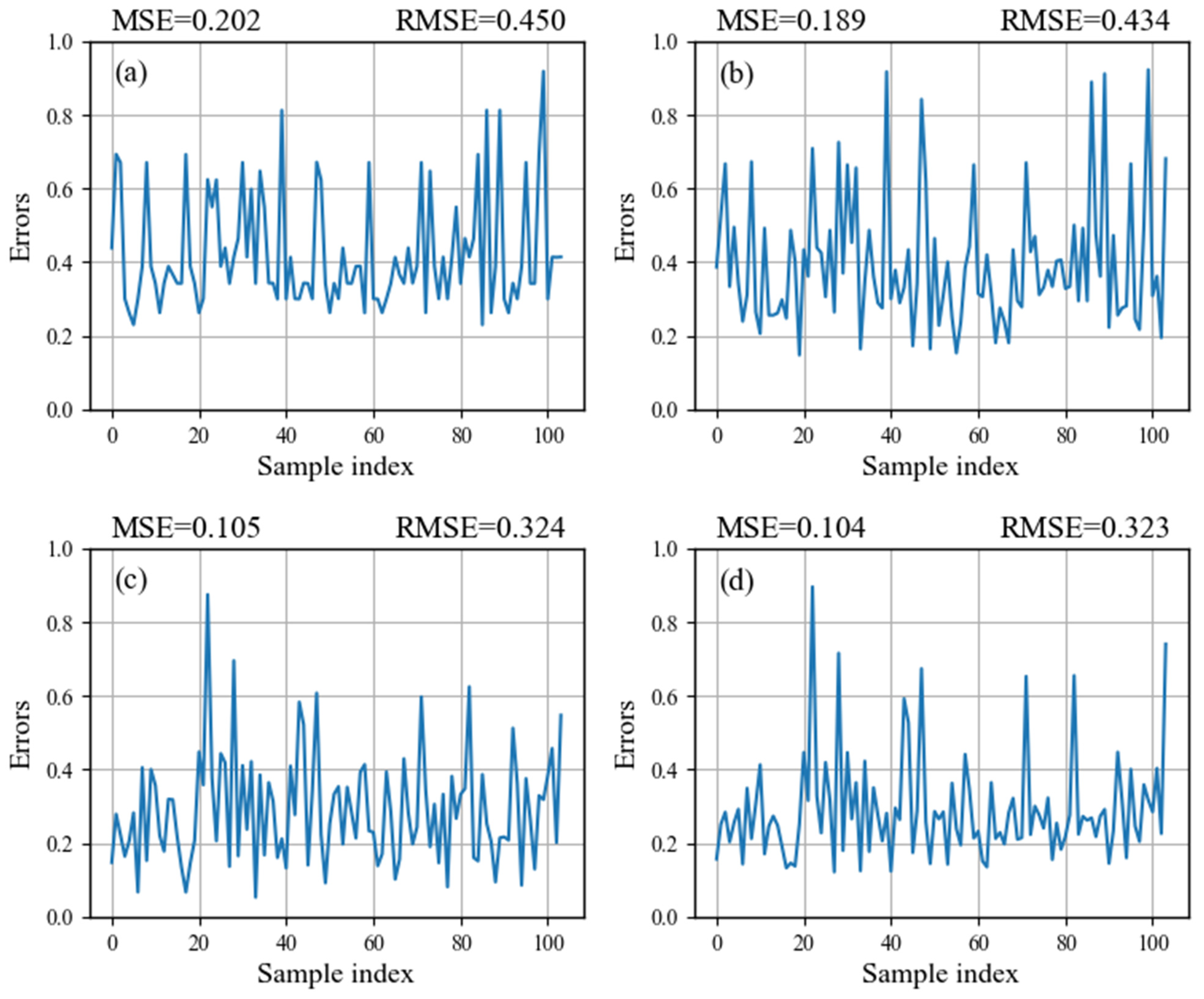
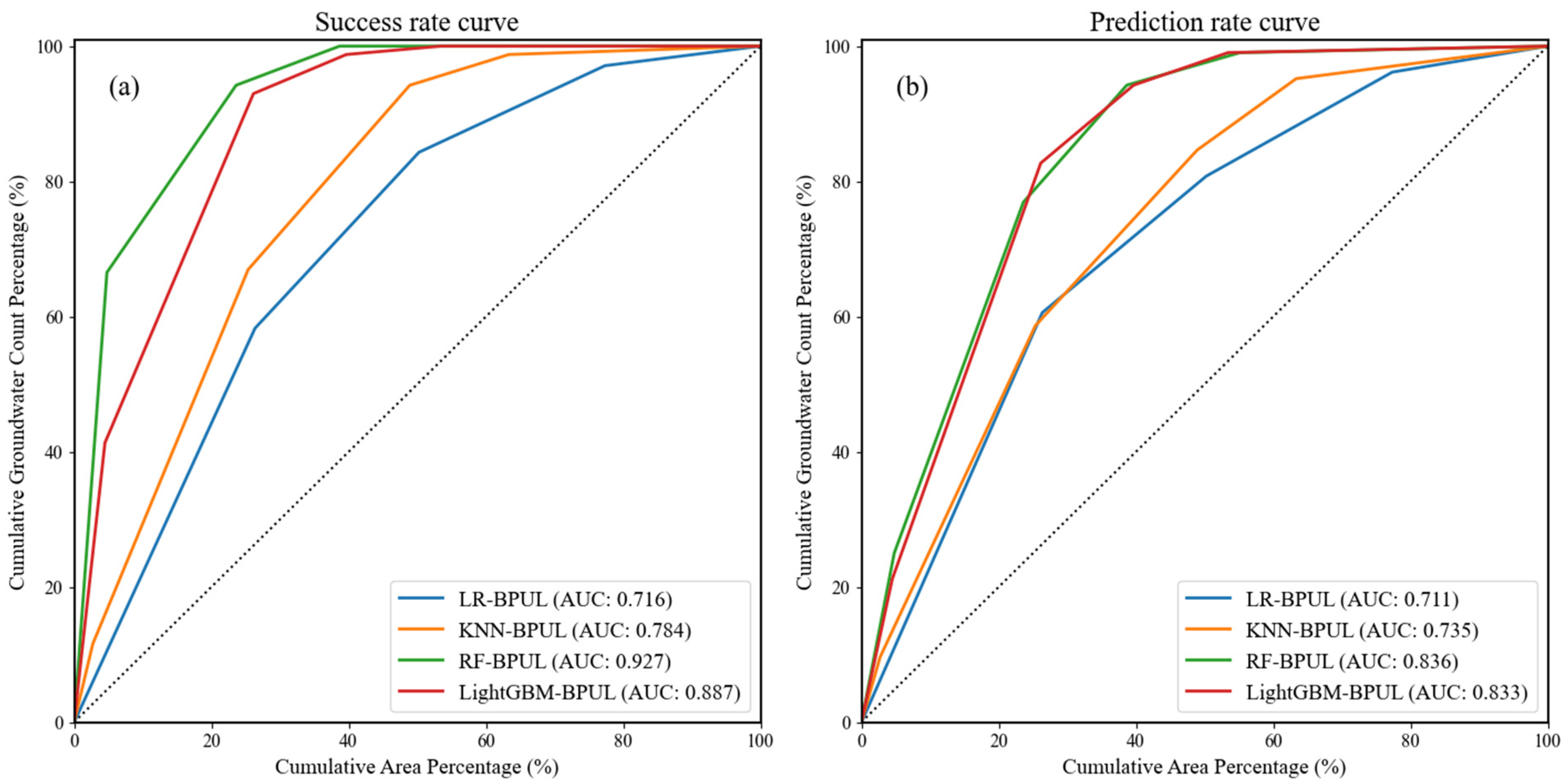
4.2. Model Evaluation and Analysis

We utilized LR, KNN, RF, and LightGBM as the base learners, which were integrated into the BPUL algorithm. The model hyper-parameters were selected as detailed in

Table 5. Hyper-parameter settings of the models.

Model Name	Common Hyper-Parameter	Hyper-Parameter of the Base Learner
LR-BPUL	n_estimators = 30, n_jobs = −1, max_samples = sum(y)	penalty = ‘l2’, C = 0.2, random_state = None, solver = ‘lbfgs’
KNN-BPUL		n_neighbors = 12, leaf_size = 10, metric = ‘minkowski’, p = 2
RF-BPUL		n_estimators = 40, random_state = 0
LightGBM-BPUL		Boosting = ‘gbdt’, colsample_bytree = 0.9, max_depth = 8, metric = ‘auc’, min_child_samples = 10, n_estimators = 40, num_leaves = 17, objective = ‘binary’, reg_lambda = 0.3, subsample = 0.9, verbose = −1

. Figure 7 represents the MSE and RMSE between the target and output for the four model test sets. Additionally, the success rate curves and prediction rate curves of the models were plotted through the training and test datasets, and the AUC values were calculated (Figure 8). The figures in

Table 6. Evaluation indexes of four models.

NO.	Model	A	F	MSE	RMSE	SRC_AUC	PRC_AUC
1	LR-BPUL	0.769	0.870	0.202	0.450	0.716	0.711
2	KNN-BPUL	0.827	0.905	0.189	0.434	0.784	0.735
3	RF-BPUL	0.914	0.955	0.105	0.324	0.927	0.836
4	LightGBM-BPUL	0.923	0.960	0.104	0.323	0.887	0.833

demonstrate the performance of the model outputs relative to the target. Overall, all four models exhibited acceptable prediction accuracy, while the hybrid ensemble models (RF-BPUL and LightGBM-BPUL) achieved higher validation scores.

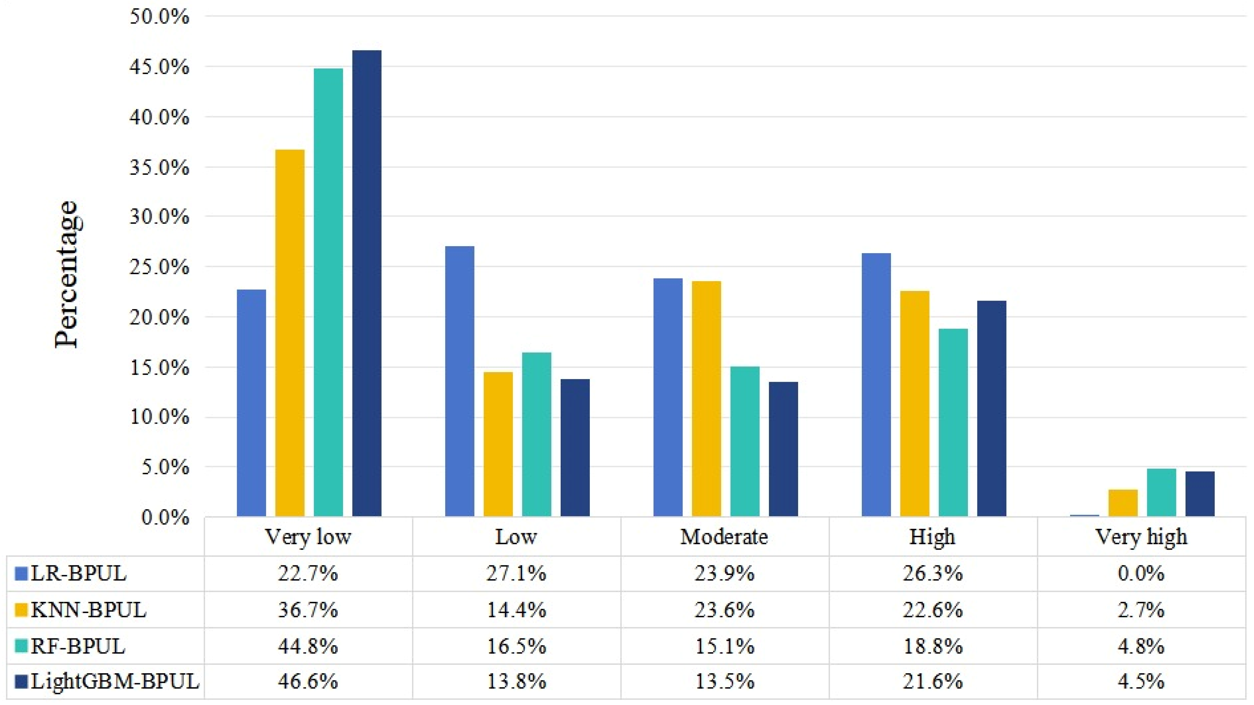
4.3. Groundwater Potential Spatial Modelling

The groundwater conditional factors in the study area served as input variables for the optimized BPUL model. This process yielded probability values for the predicted outcomes of the four distinct models, which represent the groundwater potential index. Groundwater potential maps were subsequently developed from the calculated indices and zoned into five categories using the equal interval method.

As illustrated in Figure 9, the groundwater potential maps generated by four BPUL hybrid models show a similar distribution pattern. These predictive maps effectively indicate groundwater potential across the study region. Regions classified as high–very high potential are concentrated in the central and southern parts of the Lijiang River Basin, characterized by lower elevation and karst geological formations. In contrast, areas identified as low–very low groundwater potential are primarily found in the northern sector and the high-elevation mountainous regions bordering the Lijiang River Basin, where granite and clastic rocks are prevalent. This spatial distribution highlights the significant potential of karst formations as aquifers.

We conducted a statistical analysis of the groundwater potential distributions produced by four hybrid models. As illustrated in Figure 10, approximately 50–60% of the groundwater pixels fall within low–very low potential areas, while about 25% are located in high–very high potential areas. The RF-BPUL and LightGBM-BPUL models exhibit a greater distribution of data in the very low and very high potential zones, leading to improved differentiation in the prediction results for groundwater potential zones. In contrast, the LR-BPUL and KNN-BPUL models demonstrate more ambiguity in their predictions, as their estimated probabilities for groundwater potential zones are more concentrated around moderate values.

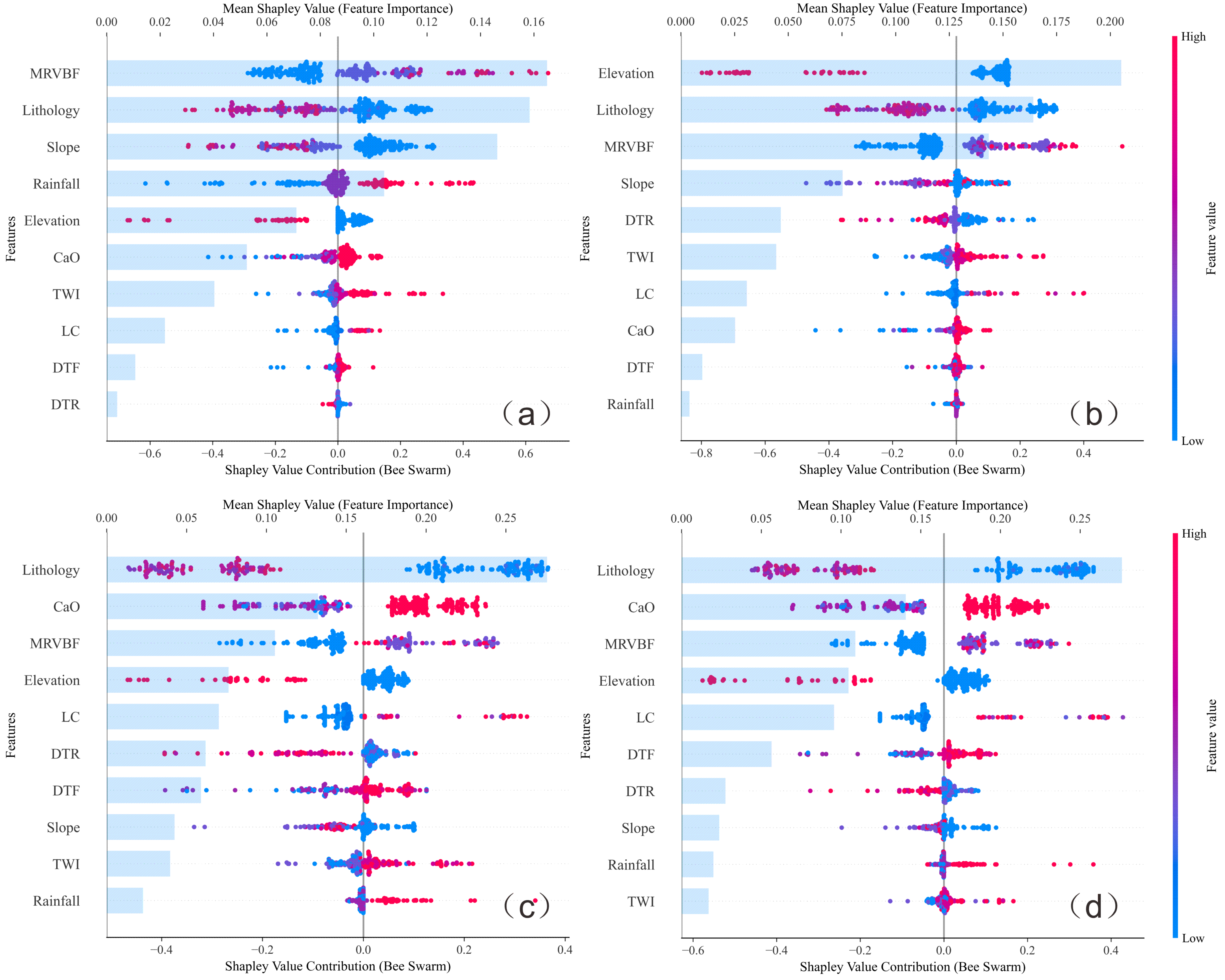
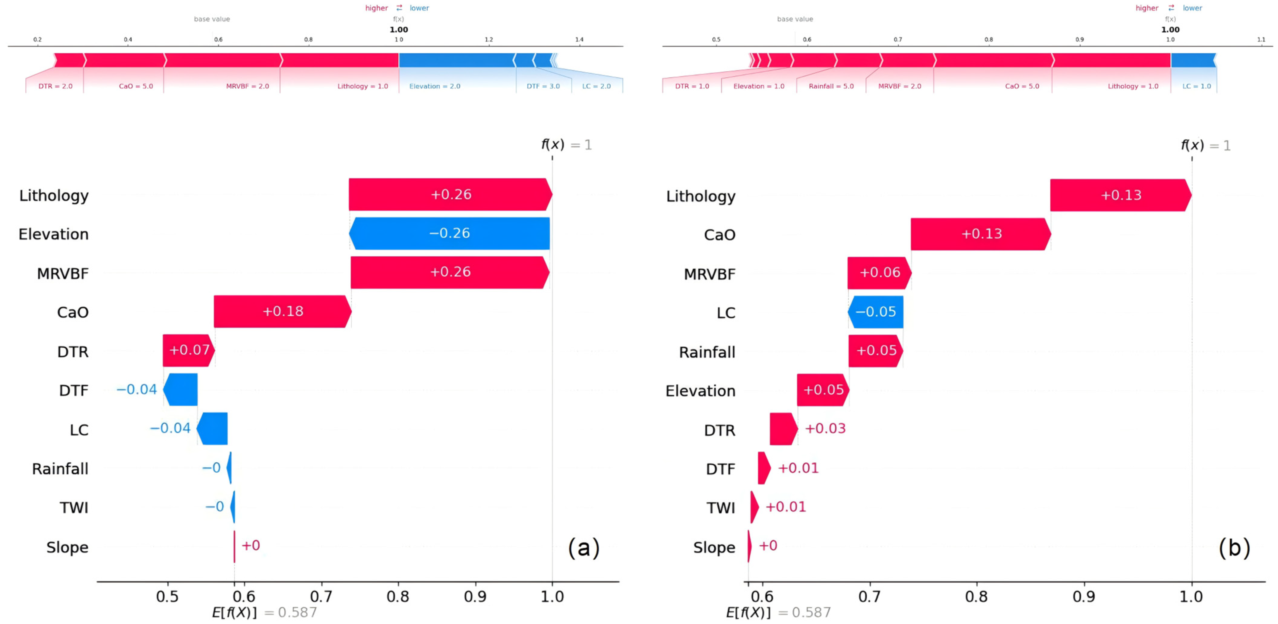
4.4. Model Interpretability in Groundwater Potential Mapping

The comprehensive SHAP value analysis of the training dataset is depicted in Figure 11, revealing feature contributions through both individual and mean SHAP values across all four models. The graph displays individual feature contributions to the model prediction, as well as its average feature importance. The hive plot beeswarm visualizes the distribution of SHAP values for each feature along the lower X-axis, with colors representing the magnitude of the feature values. In contrast, the bar chart presents the average SHAP value for each feature along the upper X-axis, ranking their importance. The analysis depicted in the figure reveals that the LR- and KNN-based BPUL models are predominantly influenced by lithology, MRVBF, elevation, and slope. In contrast, the RF- and LightGBM-based BPUL models are primarily affected by lithology, CaO, elevation, and MRVBF. This suggests that model weights is predominantly influenced by lithology, elevation, and MRVBF. Additionally, the LR-BPUL and KNN-BPUL models emphasize the influence of slope, while the RF-BPUL and LightGBM-BPUL models downplay the impact of slope and instead focus on the role of CaO in groundwater enrichment.

In addition, none of the four models disregarded the effects of elevation and land cover, indicating that topographic conditions have significant influences on groundwater storage. Furthermore, land use status also substantially affects the identification of groundwater enrichment zones.

Notably, rainfall is identified as a relatively insignificant factor in our models, exerting minimal influence on the predicted results—a finding that diverges from traditional perspectives. This can be attributed to several potential mechanisms. Firstly, the effect of precipitation on groundwater enrichment tends to be less pronounced in small-scale regional contexts, as the spatial scale of the study area may be insufficient to capture significant rainfall heterogeneity. Furthermore, the complexity of the groundwater circulation system in karst regions plays a critical role. In such areas, groundwater recharge sources are often geographically distant from the zones of groundwater enrichment. Precipitation percolates through diverse fracture pathways in carbonate rock and overlying strata lacking impermeable barriers. This process likely constitutes a major mechanism for karst groundwater recharge [69,70].

We also used SHAP to assess the local interpretability of the results, further elucidating the impact of each conditional factor on the prediction outcomes for specific samples. Figure 12 presents the SHAP force plots and waterfall plots for sample 95 (well) and sample 66 (subterranean stream) from the BPUL-LightGBM model, respectively. Regarding the color coding, red indicates a positive impact, signifying that groundwater enrichment zones in the sample region are more susceptible to these factors, while blue indicates a negative impact, suggesting that these factors exert an inhibitory effect on groundwater enrichment. At sampling point 95, lithology = 1 (indicating pure carbonates), MRVBF = 2 (ranging from 0.60 to 2.00), and CaO = 5 (ranging from 3.13 to 6.41) all contribute to an increase in the predicted value. Conversely, variables such as elevation = 2 (ranging from 278 to 487) cause a downward trend in the prediction. Similarly, at sampling point 66, pure carbonates, high CaO values, and low MRVBF values contribute to an increase in the predicted value. Moreover, abundant rainfall and low elevation are also indicative factors for identifying groundwater enrichment zones. In summary, regardless of whether the samples are from wells or subterranean streams, lithology, MRVBF, and CaO have significant impacts on the identification of groundwater enrichment zones in karst regions.

5. Discussion

5.1. Factors Driving Groundwater Enrichment in Karst Areas

To evaluate the impact of individual drivers on groundwater potential, we employed the Partial Dependence Plot (PDP) for the LightGBM-BPUL model. This approach enabled us to track the influence of various features on model predictions, thereby enhancing our understanding of the model’s operation. As illustrated in Figure 13, the analysis reveals the relationship between six major factors—lithology, CaO, elevation, MRVBF, slope, and land cover—and groundwater potential in karst areas. In the figure, the x-axis represents the range of values for the conditional factors. It should be noted that the conditional factors have been standardized in this study to eliminate the influence of scale differences among the indicators. The y-axis denotes the expected value of groundwater potential under various conditional factors. The blue line illustrates the trend of groundwater potential across different ranges of the drivers. By observing the trend of the blue line, we can discern the influence of each driver on groundwater potential predictions. The grey bars indicate the distribution of sample points for the various ranges of each driver. The dashed lines represent the expected values of the characteristic and target variables, i.e., the global average.

The isolation plot of PDP for lithology reveals distinct correlations between lithostratigraphic configurations and aquifer productivity potential. Specifically, the predictive framework demonstrates significantly elevated expectations of groundwater potential in areas characterized within geological units dominated by predominantly pure and sub-pure carbonate formations, where enhanced secondary porosity facilitates preferential groundwater recharge pathways. Conversely, it displays a very low expectation of groundwater potential in regions with impure carbonate formations, overlying carbonate rocks, and non-carbonate rocks, reflecting the combined impacts of reduced infiltration capacity and increased subsurface flow resistance associated with these geological assemblages. This suggests that pure and sub-pure carbonate formations serve as significant prerequisites for groundwater enrichment in karst areas. Furthermore, the local dependence plot for CaO indicates that when CaO is sufficiently abundant in the karst geochemistry (≥3.13%), the potential for groundwater development significantly increases. Another factor exhibiting a clearly positive correlation is MRVBF. The MRVBF index identifies relatively flat and lower areas of the landscape across various scales. It suggests that flatter valley bottom topography is more conducive to groundwater storage, whereas steeper ridge topography serves primarily as a recharge and transport zone due to the hydraulic gradient, which hinders water retention in the landscape. Similarly, the dependency plot curves for elevation and slope illustrate this mechanism of topographic influence. Among the two land use categories, cropland and woodland, the sample count is highest; however, the expectation of SHAP values is low, indicating that these two land types exert minimal influence on groundwater potential.

5.2. Strengths and Limitations of PUL Models

The Positive–Unlabeled learning model employed in this study can generate predictions that yield satisfactory results without providing negative samples. This approach addresses the challenge of collecting groundwater samples without negative samples compared to traditional applications of machine learning methods. It eliminates the uncertainty associated with constructing balanced groundwater and non-groundwater samples, thereby enhancing the credibility of the model inputs. We compared the F-scores of LightGBM using various sampling strategies with LightGBM-BPUL. A buffer zone of 1 km was established around the known positive samples, and equal numbers of points were randomly assigned as negative samples outside this buffer zone to be input into the LightGBM model. This process was repeated 10 times. Figure 14a illustrates the comparison of the F-scores of the model with a positive-to-negative sampling ratio of 1:1 across 10 random samplings. The results indicate that, although the model’s performance exhibits some fluctuations, it generally maintains an optimal state. We also used four different datasets with varying positive-to-negative sample ratios—1:1, 1:2, 1:5, and 1:10—as training sets for the LightGBM model. The results indicate that, as the number of negative samples increases, the model’s prediction accuracy consistently declines, as illustrated in Figure 14b. By randomly selecting non-groundwater samples from areas outside the known groundwater points, this selection process may inadvertently include incorrect samples, leading to biases and uncertainties. As the proportion of negative samples rises, the likelihood of such errors is amplified. Consequently, the advantages of employing Positive–Unlabeled learning (PUL) become increasingly apparent. In mineral potential prediction, the sensitivity of the PUL algorithm to different training sets of labeled and unlabeled locations has been studied: the prediction results from 10 randomly unlabeled datasets confirm that PUL modelling with different training sets is repeatable and stable [71]. In research on landslide susceptibility prediction, the effectiveness of bagging PU learning in improving the recall rate of landslides and the generalization ability of the model on imbalanced datasets has also been emphasized [72].

In addition, the construction of hybrid models demonstrates significant potential for improving the performance of maximum likelihood models. Among the four PUL-based hybrid models, those based on ensemble machine learning algorithms (RF, LightGBM) consistently outperformed models based on single machine learning algorithms (LR, KNN) across all metrics. In larger study areas with more complex environments, ensemble hybrid learning utilizes base learners to address the deficiencies in the learning process of the base model, resulting in enhanced predictive capabilities.

However, the absence of a reliable test set of negative samples leads to an evaluation of the model that is not yet comprehensive, which remains a limitation of this paper and should be acknowledged. Therefore, in the future, we will continue to study the application of the PUL model in groundwater potential prediction and develop more scientifically robust evaluation metrics to assess the model’s performance more thoroughly. Additionally, it is essential that future research focuses on the development of additional groundwater condition factors with enhanced accuracy. Comprehensive datasets enable models to capture finer details and improve their accuracy, which is crucial for studying the highly heterogeneous nature of groundwater distribution in karst regions.

6. Conclusions

In complex karst regions, the scarcity of boreholes and wells significantly limits the availability of groundwater training samples for machine learning, particularly when reliable negative samples are lacking. To address these challenges, this study pioneers the application of a Positive–Unlabeled learning-based hybrid model for groundwater potential mapping in karst areas, with a case study in the Lijiang River Basin. Our experimental results yield the following key findings:

(1)

The BPUL algorithm, integrated with four base learners (LR, KNN, RF, and LightGBM) effectively overcame the scarcity of negative samples by leveraging positive and unlabeled data, achieving satisfactory prediction results across all models. Among them, the hybrid ensemble models (RF-BPUL and LightGBM-BPUL) exhibited superior performance, as evidenced by their higher validation scores.

(2)

Through evaluating the correlations and SHAP values of groundwater conditional factors, we identified lithology (particularly pure carbonate rocks), MRVBF, and CaO content as critical drivers of groundwater enrichment in karst zones.

In conclusion, the significance of this research lies in its pioneering use of Positive–Unlabeled learning-based hybrid models for groundwater potential mapping. Additionally, it introduces two new influential factors, CaO and MRVBF, into the groundwater potential modelling of karst regions. This approach provides an efficient and reliable framework for mapping groundwater potential in karst areas. Future research could further focus on developing more comprehensive evaluation metrics for the framework and exploring additional groundwater conditional factors, thereby enhancing the model’s robustness across diverse karst landscapes.

References

1. Scanlon, B.R.; Fakhreddine, S.; Rateb, A.; de Graaf, I.; Famiglietti, J.; Gleeson, T.; Grafton, R.Q.; Jobbagy, E.; Kebede, S.; Kolusu, S.R.; et al. Global water resources and the role of groundwater in a resilient water future. Nat. Rev. Earth Environ. 2023, 4, 87–101. [Google Scholar] [CrossRef]
2. Pointet, T. The United Nations World Water Development Report 2022 on groundwater, a synthesis. Lhb 2022, 108, 2090867. [Google Scholar] [CrossRef]
3. Famiglietti, J.S. The global groundwater crisis. Nat. Clim. Chang. 2014, 4, 945–948. [Google Scholar] [CrossRef]
4. Panahi, M.; Sadhasivam, N.; Pourghasemi, H.R.; Rezaie, F.; Lee, S. Spatial prediction of groundwater potential mapping based on convolutional neural network (CNN) and support vector regression (SVR). J. Hydrol. 2020, 588, 125033. [Google Scholar] [CrossRef]
5. Thanh, N.N.; Thunyawatcharakul, P.; Ngu, N.H.; Chotpantarat, S. Global review of groundwater potential models in the last decade: Parameters, model techniques, and validation. J. Hydrol. 2022, 614, 128501. [Google Scholar] [CrossRef]
6. Díaz-Alcaide, S.; Martínez-Santos, P. Review: Advances in groundwater potential mapping. Hydrogeol. J. 2019, 27, 2307–2324. [Google Scholar] [CrossRef]
7. Binley, A.; Hubbard, S.S.; Huisman, J.A.; Revil, A.; Robinson, D.A.; Singha, K.; Slater, L.D. The emergence of hydrogeophysics for improved understanding of subsurface processes over multiple scales. Water Resour. Res. 2015, 51, 3837–3866. [Google Scholar] [CrossRef]
8. Wang, D.; Qian, J.; Ma, L.; Xu, H.; Wang, X.; Wang, Y. Integration of multiple hydrogeological survey technologies for exploring the groundwater distribution in karst areas: A case study in Xingfu Spring, Chaohu City, China. J. Hydrol. 2022, 614, 128637. [Google Scholar] [CrossRef]
9. Luo, M.; Chen, Z.; Zhou, H.; Jakada, H.; Zhang, L.; Han, Z.; Shi, T. Identifying structure and function of karst aquifer system using multiple field methods in karst trough valley area, South China. Environ. Earth Sci. 2016, 75, 824. [Google Scholar] [CrossRef]
10. Pourmorad, S.; Abbasi, S.; Patel, N.; Mohanty, A. Investigation and Potential Identification of Karsts as Groundwater Resources with the Help of GIS Studies, a Case Study of Western Iran. Lithol. Miner. Resour. 2022, 57, 584–599. [Google Scholar] [CrossRef]
11. Opoku, P.A.; Shu, L.; Amoako-Nimako, G.K. Assessment of Groundwater Potential Zones by Integrating Hydrogeological Data, Geographic Information Systems, Remote Sensing, and Analytical Hierarchical Process Techniques in the Jinan Karst Spring Basin of China. Water 2024, 16, 565. [Google Scholar] [CrossRef]
12. Ally, A.M.; Yan, J.; Bennett, G.; Lyimo, N.N.; Mayunga, S.D. Assessment of groundwater potential zones using remote sensing and GIS-based fuzzy analytical hierarchy process (F-AHP) in Mpwapwa District, Dodoma, Tanzania. Geosystems Geoenvironment 2024, 3, 100232. [Google Scholar] [CrossRef]
13. Arabameri, A.; Rezaei, K.; Cerda, A.; Lombardo, L.; Rodrigo-Comino, J. GIS-based groundwater potential mapping in Shahroud plain, Iran. A comparison among statistical (bivariate and multivariate), data mining and MCDM approaches. Sci. Total Environ. 2019, 658, 160–177. [Google Scholar] [CrossRef] [PubMed]
14. Çelik, M.Ö.; Kuşak, L.; Yakar, M. Assessment of Groundwater Potential Zones Utilizing Geographic Information System-Based Analytical Hierarchy Process, Vlse Kriterijumska Optimizacija Kompromisno Resenje, and Technique for Order Preference by Similarity to Ideal Solution Methods: A Case Study in Mersin, Türkiye. Sustainability 2024, 16, 2202. [Google Scholar] [CrossRef]
15. Ferretti, V.; Montibeller, G. Key challenges and meta-choices in designing and applying multi-criteria spatial decision support systems. Decis. Support Syst. 2016, 84, 41–52. [Google Scholar] [CrossRef]
16. Rizeei, H.M.; Pradhan, B.; Saharkhiz, M.A.; Lee, S. Groundwater aquifer potential modeling using an ensemble multi-adoptive boosting logistic regression technique. J. Hydrol. 2019, 579, 124172. [Google Scholar] [CrossRef]
17. Jari, A.; Bachaoui, E.M.; Hajaj, S.; Khaddari, A.; Khandouch, Y.; El Harti, A.; Jellouli, A.; Namous, M. Investigating machine learning and ensemble learning models in groundwater potential mapping in arid region: Case study from Tan-Tan water-scarce region, Morocco. Front. Water 2023, 5, 1305998. [Google Scholar] [CrossRef]
18. Khosravi, K.; Panahi, M.; Tien Bui, D. Spatial prediction of groundwater spring potential mapping based on an adaptive neuro-fuzzy inference system and metaheuristic optimization. Hydrol. Earth Syst. Sci. 2018, 22, 4771–4792. [Google Scholar] [CrossRef]
19. Naghibi, S.A.; Ahmadi, K.; Daneshi, A. Application of Support Vector Machine, Random Forest, and Genetic Algorithm Optimized Random Forest Models in Groundwater Potential Mapping. Water Resour. Manag. 2017, 31, 2761–2775. [Google Scholar] [CrossRef]
20. Pham, B.T.; Jaafari, A.; Prakash, I.; Singh, S.K.; Quoc, N.K.; Bui, D.T. Hybrid computational intelligence models for groundwater potential mapping. Catena 2019, 182, 104101. [Google Scholar] [CrossRef]
21. Guo, X.; Gui, X.; Xiong, H.; Hu, X.; Li, Y.; Cui, H.; Qiu, Y.; Ma, C. Critical role of climate factors for groundwater potential mapping in arid regions: Insights from random forest, XGBoost, and LightGBM algorithms. J. Hydrol. 2023, 621, 129599. [Google Scholar] [CrossRef]
22. Ragragui, H.; Aouragh, M.H.; El-Hmaidi, A.; Ouali, L.; Saouita, J.; Iallamen, Z.; Ousmana, H.; Jaddi, H.; El Ouali, A. Mapping and modeling groundwater potential using machine learning, deep learning and ensemble learning models in the Saiss basin (Fez-Meknes region, Morocco). Groundw. Sustain. Dev. 2024, 26, 101281. [Google Scholar] [CrossRef]
23. Mohammed, A.; Kora, R. A comprehensive review on ensemble deep learning: Opportunities and challenges. J. King Saud. Univ. Comput. Inf. Sci. 2023, 35, 757–774. [Google Scholar] [CrossRef]
24. Kamali Maskooni, E.; Naghibi, S.A.; Hashemi, H.; Berndtsson, R. Application of Advanced Machine Learning Algorithms to Assess Groundwater Potential Using Remote Sensing-Derived Data. Remote Sens. 2020, 12, 2742. [Google Scholar] [CrossRef]
25. Nykänen, V.; Lahti, I.; Niiranen, T.; Korhonen, K. Receiver operating characteristics (ROC) as validation tool for prospectivity models—A magmatic Ni–Cu case study from the Central Lapland Greenstone Belt, Northern Finland. Ore Geol. Rev. 2015, 71, 853–860. [Google Scholar] [CrossRef]
26. Fang, Z.; Wang, Y.; Niu, R.; Peng, L. Landslide Susceptibility Prediction Based on Positive Unlabeled Learning Coupled with Adaptive Sampling. IEEE J.-Stars 2021, 14, 11581–11592. [Google Scholar] [CrossRef]
27. Gu, T.; Duan, P.; Wang, M.; Li, J.; Zhang, Y. Effects of non-landslide sampling strategies on machine learning models in landslide susceptibility mapping. Sci. Rep. 2024, 14, 7201. [Google Scholar] [CrossRef]
28. Bekker, J.; Davis, J. Learning from positive and unlabeled data: A survey. Mach. Learn. 2020, 109, 719–760. [Google Scholar] [CrossRef]
29. Gao, M.; Wang, G.; Yang, W.; Zhang, Z.; Cai, D.; Xu, Y.; Yang, S. Bagging-based Positive–Unlabeled Data Learning Algorithm with Base Learners Random Forest and XGBoost for 3D Exploration Targeting in the Kalatongke District, Xinjiang, China. Nat. Resour. Res. 2023, 32, 437–459. [Google Scholar] [CrossRef]
30. Zhang, Z.; Wang, G.; Liu, C.; Cheng, L.; Sha, D. Bagging-based positive-unlabeled learning algorithm with Bayesian hyperparameter optimization for three-dimensional mineral potential mapping. Comput. Geosci. 2021, 154, 104817. [Google Scholar] [CrossRef]
31. Wu, B.; Qiu, W.; Jia, J.; Liu, N. Landslide Susceptibility Modeling Using Bagging-Based Positive-Unlabeled Learning. IEEE Geosci. Remote S 2021, 18, 766–770. [Google Scholar] [CrossRef]
32. Waltham, T. Guangxi Karst: The Fenglin and Fengcong Karst of Guilin and Yangshuo. In Geomorphological Landscapes of the World; Migon, P., Ed.; Springer: Dordrecht, The Netherlands, 2010; pp. 293–302. [Google Scholar]
33. Dai-zhao, C.; Hai-ruo, Q. Devonian-Carboniferous Carbonates in Guilin, South China: Depositional Records of Platform-Basin Complex and Major Biocrisises. In Field Trip Guidebook on Chinese Sedimentary Geology; Hu, X., Ed.; Springer Nature: Singapore, 2024; pp. 809–871. [Google Scholar]
34. Pu, Z.; Huang, Q.; Liao, H.; Wu, H.; Jiao, Y.; Luo, F.; Li, T.; Zhao, G.; Zou, C. Underground karst development characteristics and their influence on exploitation of karst groundwater in Guilin City, southwestern China. Carbonate Evaporite 2024, 39, 34. [Google Scholar] [CrossRef]
35. Saha, A.; Saha, S. Comparing the efficiency of weight of evidence, support vector machine and their ensemble approaches in landslide susceptibility modelling: A study on Kurseong region of Darjeeling Himalaya, India. Remote Sens. Appl. Soc. Environ. 2020, 19, 100323. [Google Scholar] [CrossRef]
36. Miraki, S.; Zanganeh, S.H.; Chapi, K.; Singh, V.P.; Shirzadi, A.; Shahabi, H.; Pham, B.T. Mapping Groundwater Potential Using a Novel Hybrid Intelligence Approach. Water Resour. Manag. 2019, 33, 281–302. [Google Scholar] [CrossRef]
37. Kalantar, B.; Al-Najjar, H.; Pradhan, B.; Saeidi, V.; Halin, A.A.; Ueda, N.; Naghibi, S.A. Optimized Conditioning Factors Using Machine Learning Techniques for Groundwater Potential Mapping. Water 2019, 11, 1909. [Google Scholar] [CrossRef]
38. Zhao, R.; Fan, C.C.; Arabameri, A.; Santosh, M.; Mohammad, L.; Mondal, I. Groundwater spring potential mapping: Assessment the contribution of hydrogeological factors. Adv. Space Res. 2024, 74, 48–64. [Google Scholar] [CrossRef]
39. Morbidelli, R.; Saltalippi, C.; Flammini, A.; Govindaraju, R.S. Role of slope on infiltration: A review. J. Hydrol. 2018, 557, 878–886. [Google Scholar] [CrossRef]
40. Iwahashi, J.; Pike, R.J. Automated classifications of topography from DEMs by an unsupervised nested-means algorithm and a three-part geometric signature. Geomorphology 2007, 86, 409–440. [Google Scholar] [CrossRef]
41. Gallant, J.C.; Dowling, T.I. A multiresolution index of valley bottom flatness for mapping depositional areas. Water Resour. Res. 2003, 39, 1347. [Google Scholar] [CrossRef]
42. Pourghasemi, H.R.; Sadhasivam, N.; Yousefi, S.; Tavangar, S.; Ghaffari Nazarlou, H.; Santosh, M. Using machine learning algorithms to map the groundwater recharge potential zones. J. Environ. Manag. 2020, 265, 110525. [Google Scholar] [CrossRef]
43. Moore, I.D.; Grayson, R.B.; Ladson, A.R. Digital terrain modelling: A review of hydrological, geomorphological, and biological applications. Hydrol. Process. 1991, 5, 3–30. [Google Scholar] [CrossRef]
44. Guduru, J.U.; Jilo, N.B. Groundwater potential zone assessment using integrated analytical hierarchy process-geospatial driven in a GIS environment in Gobele watershed, Wabe Shebele river basin, Ethiopia. J. Hydrol. Reg. Stud. 2022, 44, 101218. [Google Scholar] [CrossRef]
45. Beven, K.J.; Kirkby, M.J.; Freer, J.E.; Lamb, R. A history of TOPMODEL. Hydrol. Earth Syst. Sci. 2021, 25, 527–549. [Google Scholar] [CrossRef]
46. Melton, M.A. The Geomorphic and Paleoclimatic Significance of Alluvial Deposits in Southern Arizona: A Reply. J. Geol. 1966, 74, 102–106. [Google Scholar] [CrossRef]
47. Arabameri, A.; Pal, S.C.; Rezaie, F.; Nalivan, O.A.; Chowdhuri, I.; Saha, A.; Lee, S.; Moayedi, H. Modeling groundwater potential using novel GIS-based machine-learning ensemble techniques. J. Hydrol. Reg. Stud. 2021, 36, 100848. [Google Scholar] [CrossRef]
48. Andualem, T.G.; Demeke, G.G. Groundwater potential assessment using GIS and remote sensing: A case study of Guna tana landscape, upper blue Nile Basin, Ethiopia. J. Hydrol. Reg. Stud. 2019, 24, 100610. [Google Scholar] [CrossRef]
49. Al-Djazouli, M.O.; Elmorabiti, K.; Rahimi, A.; Amellah, O.; Fadil, O.A.M. Delineating of groundwater potential zones based on remote sensing, GIS and analytical hierarchical process: A case of Waddai, eastern Chad. Geojournal 2021, 86, 1881–1894. [Google Scholar] [CrossRef]
50. Li, X.; Wang, Y.; Shu, L.; Wang, Y.; Tong, F.; Han, J.; Shu, W.; Li, D.; Wen, J. The controlling factors of the karst water hydrochemistry in a karst basin of southwestern China. Environ. Earth Sci. 2021, 80, 793. [Google Scholar] [CrossRef]
51. Al-Hashim, M.H.; Al-Aidaros, A.; Zaidi, F.K. Geological and Hydrochemical Processes Driving Karst Development in Southeastern Riyadh, Central Saudi Arabia. Water 2024, 16, 1937. [Google Scholar] [CrossRef]
52. Thapa, R.; Gupta, S.; Gupta, A.; Reddy, D.V.; Kaur, H. Use of geospatial technology for delineating groundwater potential zones with an emphasis on water-table analysis in Dwarka River basin, Birbhum, India. Hydrogeol. J. 2018, 26, 899–922. [Google Scholar] [CrossRef]
53. Zabidi, H.; Termizi, M.; Aliman, S.; Ariffin, K.S.; Khalil, N.L. Geological Structure and Geomorphological Aspects in Karstified Susceptibility Mapping of Limestone Formations. Procedia Chem. 2016, 19, 659–665. [Google Scholar] [CrossRef]
54. Yeh, H.; Cheng, Y.; Lin, H.; Lee, C. Mapping groundwater recharge potential zone using a GIS approach in Hualian River, Taiwan. Sustain. Environ. Res. 2016, 26, 33–43. [Google Scholar] [CrossRef]
55. Fick, S.E.; Hijmans, R.J. WorldClim 2: New 1-km spatial resolution climate surfaces for global land areas. Int. J. Clim. 2017, 37, 4302–4315. [Google Scholar] [CrossRef]
56. Tahmassebipoor, N.; Rahmati, O.; Noormohamadi, F.; Lee, S. Spatial analysis of groundwater potential using weights-of-evidence and evidential belief function models and remote sensing. Arab. J. Geosci. 2016, 9, 1–18. [Google Scholar] [CrossRef]
57. Yang, J.; Huang, X. The 30 m annual land cover dataset and its dynamics in China from 1990 to 2019. Earth Syst. Sci. Data 2021, 13, 3907–3925. [Google Scholar]
58. Farrar, D.E.; Glauber, R.R. Multicollinearity in Regression Analysis: The Problem Revisited. Rev. Econ. Stat. 1967, 49, 92–107. [Google Scholar] [CrossRef]
59. Mordelet, F.; Vert, J.P. A bagging SVM to learn from positive and unlabeled examples. Pattern Recogn. Lett. 2014, 37, 201–209. [Google Scholar] [CrossRef]
60. Sarkar, S.K.; Rudra, R.R.; Talukdar, S.; Das, P.C.; Nur, M.S.; Alam, E.; Islam, M.K.; Islam, A.R.M.T. Future groundwater potential mapping using machine learning algorithms and climate change scenarios in Bangladesh. Sci. Rep. 2024, 14, 10328. [Google Scholar] [CrossRef]
61. Huang, P.; Hou, M.; Sun, T.; Xu, H.; Ma, C.; Zhou, A. Sustainable groundwater management in coastal cities: Insights from groundwater potential and vulnerability using ensemble learning and knowledge-driven models. J. Clean. Prod. 2024, 442, 141152. [Google Scholar] [CrossRef]
62. Hanshika, V.G.; Preethi, S.; Sreemathy, S.P.; Ezhillin Freeda, S. Flood Prediction Using Logistic Regression. In Proceedings of the 2023 International Conference on Circuit Power and Computing Technologies (ICCPCT), Kollam, India, 10–11 August 2023; pp. 1174–1179. [Google Scholar]
63. Guo, Z.; Shi, Y.; Huang, F.; Fan, X.; Huang, J. Landslide susceptibility zonation method based on C5.0 decision tree and K-means cluster algorithms to improve the efficiency of risk management. Geosci. Front. 2021, 12, 101249. [Google Scholar] [CrossRef]
64. Mosavi, A.; Sajedi Hosseini, F.; Choubin, B.; Goodarzi, M.; Dineva, A.A.; Rafiei Sardooi, E. Ensemble Boosting and Bagging Based Machine Learning Models for Groundwater Potential Prediction. Water Resour. Manag. 2021, 35, 23–37. [Google Scholar] [CrossRef]
65. Zhang, J.; Ma, X.; Zhang, J.; Sun, D.; Zhou, X.; Mi, C.; Wen, H. Insights into geospatial heterogeneity of landslide susceptibility based on the SHAP-XGBoost model. J. Environ. Manag. 2023, 332, 117357. [Google Scholar] [CrossRef] [PubMed]
66. Yang, F.; Zuo, R.; Xiong, Y.; Xu, Y.; Nie, J.; Zhang, G. Dual-Branch Convolutional Neural Network and Its Post Hoc Interpretability for Mapping Mineral Prospectivity. Math. Geosci. 2024, 56, 1487–1515. [Google Scholar] [CrossRef]
67. Ribeiro, M.T.; Singh, S.; Guestrin, C. “Why Should I Trust You?”: Explaining the Predictions of Any Classifier. In Proceedings of the 22nd ACM SIGKDD International Conference on Knowledge Discovery and Data Mining, San Francisco, CA, USA, 13–17 August 2016; Association for Computing Machinery: New York, NY, USA, 2016; pp. 1135–1144. [Google Scholar]
68. Lundberg, S.M.; Lee, S. A unified approach to interpreting model predictions. In Proceedings of the 31st International Conference on Neural Information Processing Systems, Long Beach, CA, USA, 4–9 December 2017; Curran Associates Inc.: Red Hook, NY, USA, 2017; pp. 4768–4777. [Google Scholar]
69. Bakalowicz, M. Karst groundwater: A challenge for new resources. Hydrogeol. J. 2005, 13, 148–160. [Google Scholar] [CrossRef]
70. Salvadori, M.; Pennisi, M.; Masciale, R.; Fidelibus, M.D.; Frollini, E.; Ghergo, S.; Parrone, D.; Preziosi, E.; Passarella, G. Isotopic study for evaluating complex groundwater circulation patterns, hydrogeological zoning, and water-rock interaction in a Mediterranean coastal karst environment. Sci. Total Environ. 2024, 955, 176850. [Google Scholar] [CrossRef]
71. Xiong, Y.; Zuo, R. A positive and unlabeled learning algorithm for mineral prospectivity mapping. Comput. Geosci. 2021, 147, 104667. [Google Scholar] [CrossRef]
72. Zhao, L.; Ma, H.; Dong, J.; Wu, X.; Xu, H.; Niu, R. A Comparative Study of Landslide Susceptibility Mapping Using Bagging PU Learning in Class-Prior Probability Shift Datasets. Remote Sens. 2023, 15, 5547. [Google Scholar] [CrossRef]
Figure 1. Geographical distribution map of the Lijiang River Basin.
Water 17 01422 g001
Figure 2. (a) Illustration of a typical subterranean stream flow path and sampling example. (b) Photo example of a subterranean stream outlet. (c) Photo example of a karst window.
Water 17 01422 g002
Figure 3. Groundwater conditional factors: (ad) topographic factors ((a) elevation, (b) slope, (c) STI, (d) MRVBF); (eg) hydrological factors ((e) TWI, (f) MRN, (g) DTR); (hj) geological factors ((h) lithology, (i) CaO, (j) DTF); (k) meteorological factor ((k) rainfall); (l) land cover factor ((l) LC).
Water 17 01422 g003
Figure 4. The workflow of the methodology.
Water 17 01422 g004
Figure 5. Schematic diagram of the BPUL algorithm.
Water 17 01422 g005
Figure 6. Heatmap of Spearman correlation analysis.
Water 17 01422 g006
Figure 7. MSE and RMSE values of the four models using the test dataset: (a) LR-BPUL, (b) KNN-BPUL, (c) RF-BPUL, and (d) LightGBM-BPUL.
Water 17 01422 g007
Figure 8. (a) Success rate curve and (b) prediction rate curve of the four models.
Water 17 01422 g008
Figure 9. Groundwater potential maps: (a) LR-BPUL model; (b) KNN-BPUL model; (c) RF-BPUL model; (d) LightGBM-BPUL model.
Water 17 01422 g009
Figure 10. Percentages of groundwater potential classes.
Water 17 01422 g010
Figure 11. Summary SHAP value plots for LR-BPUL (a), KNN-BPUL (b), RF-BPUL (c), and LightGBM-BPUL (d).
Water 17 01422 g011
Figure 12. Local interpretability using SHAP, with force plot and waterfall plot. (a) SHAP for well location; (b) SHAP for subterranean stream location.
Water 17 01422 g012
Figure 13. Isolation plots of PDP for the six primary factors influencing the LightGBM-BPUL model.
Water 17 01422 g013
Figure 14. Comparison of F-scores between LightGBM with different sampling strategies and LightGBM-BPUL: (a) model performance comparison with 1:1 positive-to-negative sample ratio under 10 random samplings; (b) model performance comparison with different positive-to-negative sample ratios (1:1, 1:2, 1:5, and 1:10) after random sampling.
Water 17 01422 g014