
China’s Inequality in Urban and Rural Residential Water Consumption—A New Multi-Analysis System


Abstract
1. Introduction
2. Literature Review
3. Methodology
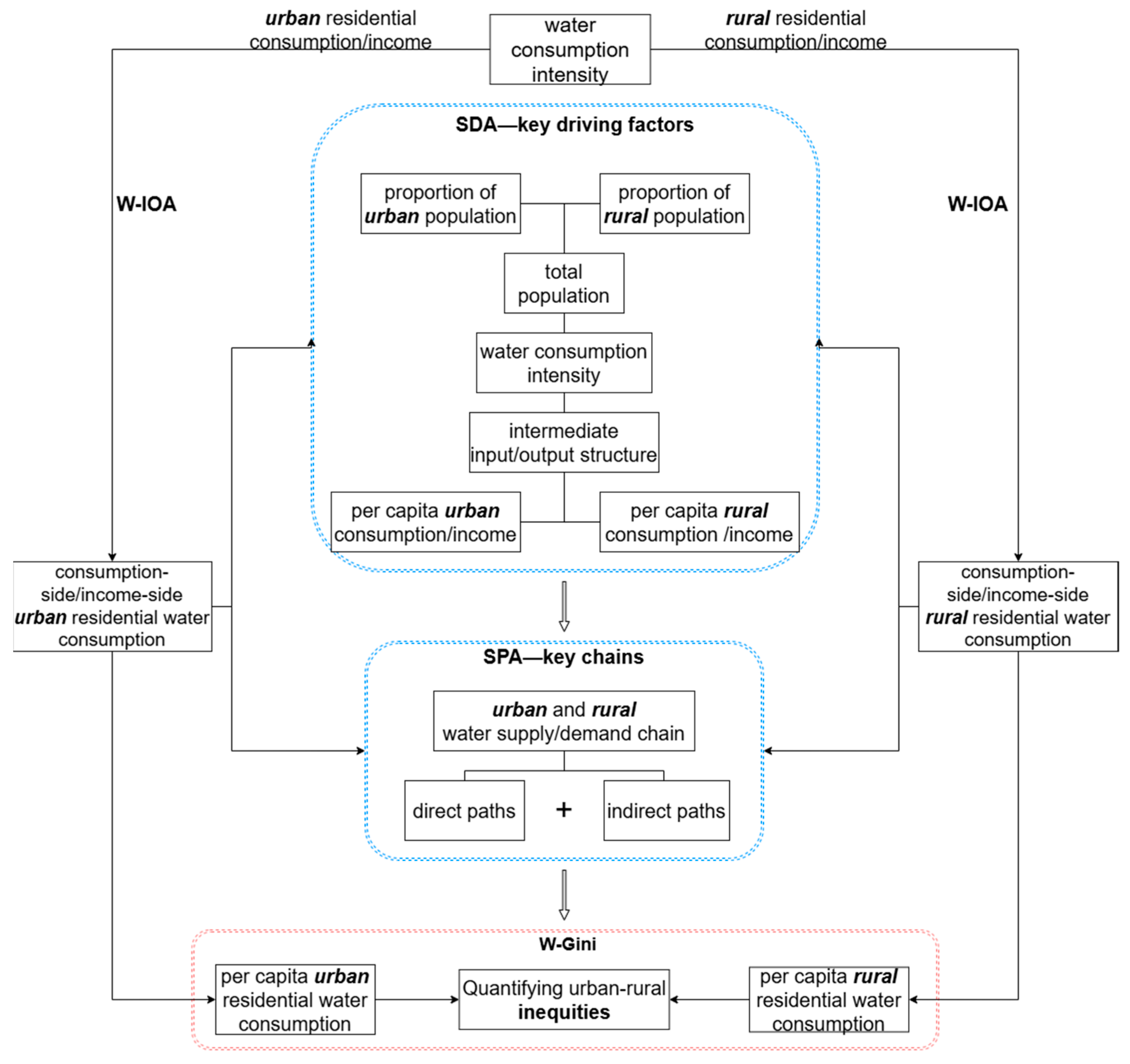
3.1. Framework
3.2. Account for Residential Water Consumption
3.3. Identify the Key Drivers
3.4. Identify the Critical Paths
3.5. Quantifying Inequities in Water Consumption
3.6. Data
4. Result and Discussion
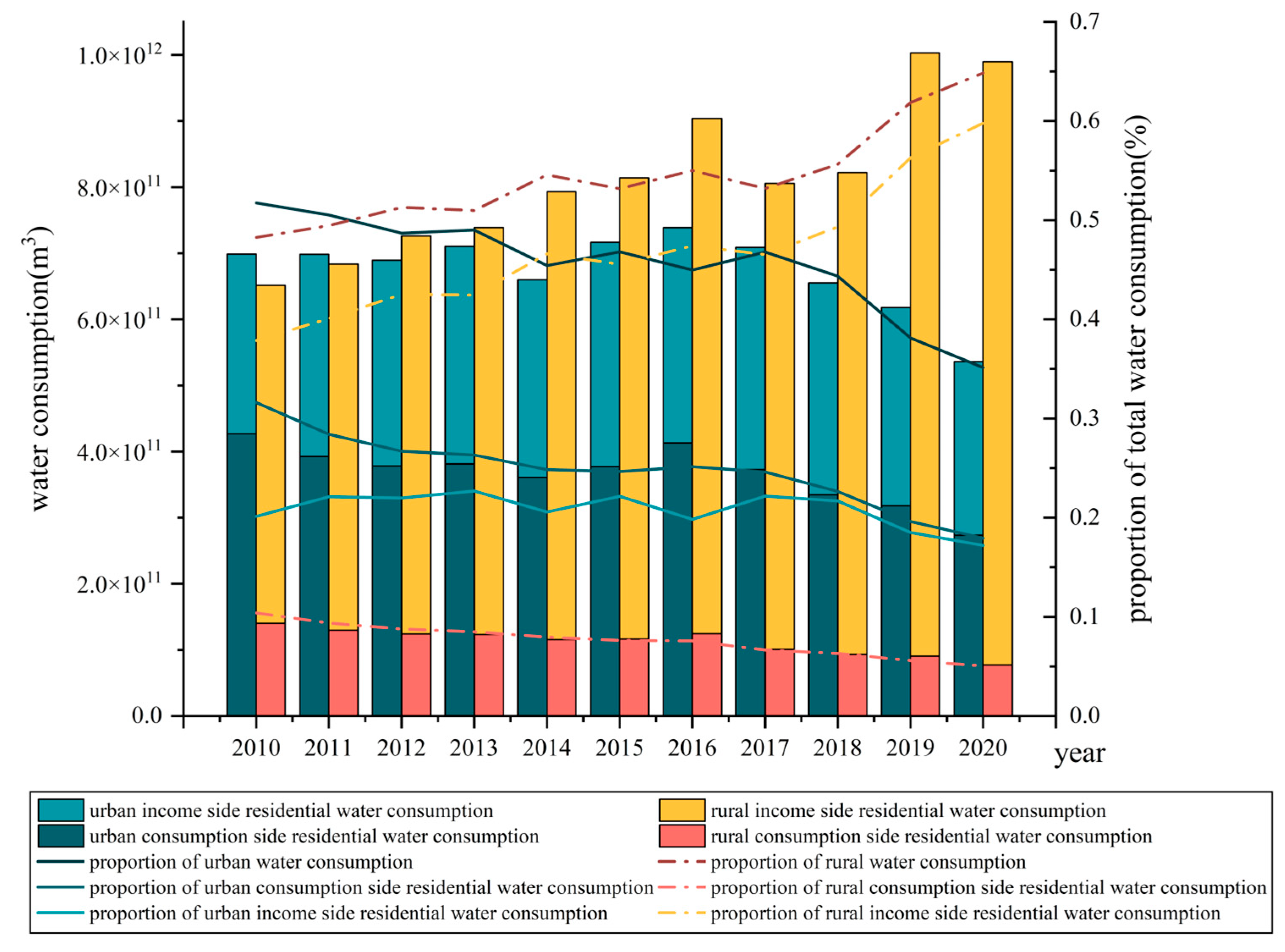
4.1. Temporal Trends in Residential Water Consumption and Driving Factors
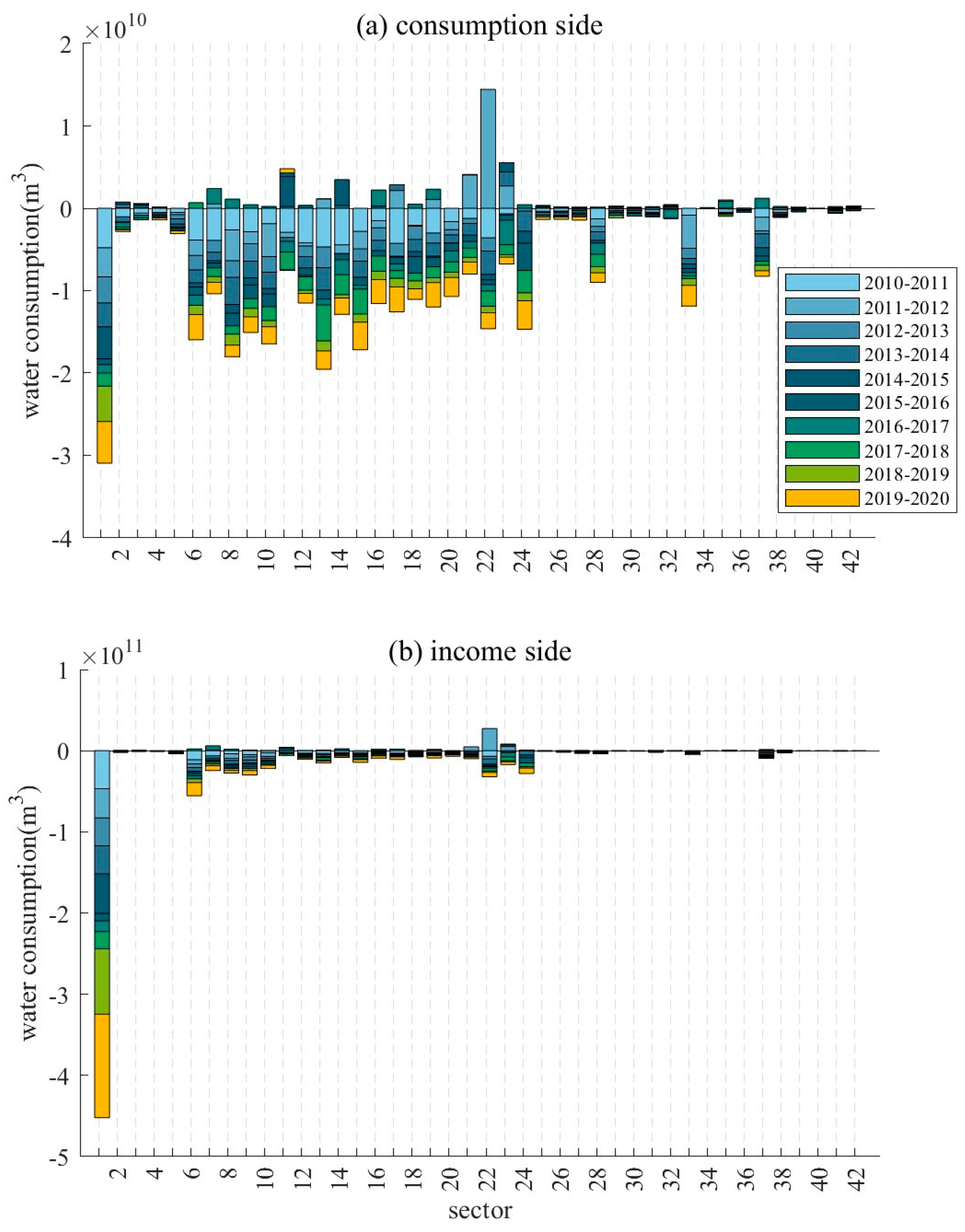
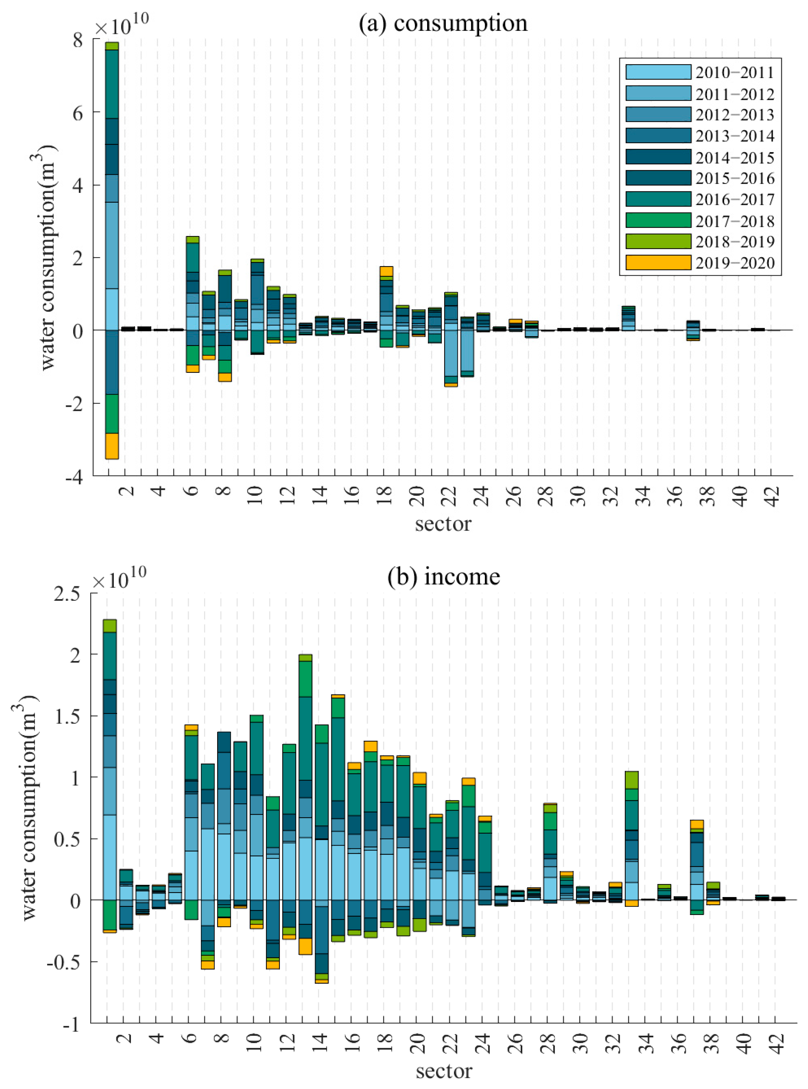
4.2. Sectoral Water Consumption Change Caused by Driving Factors
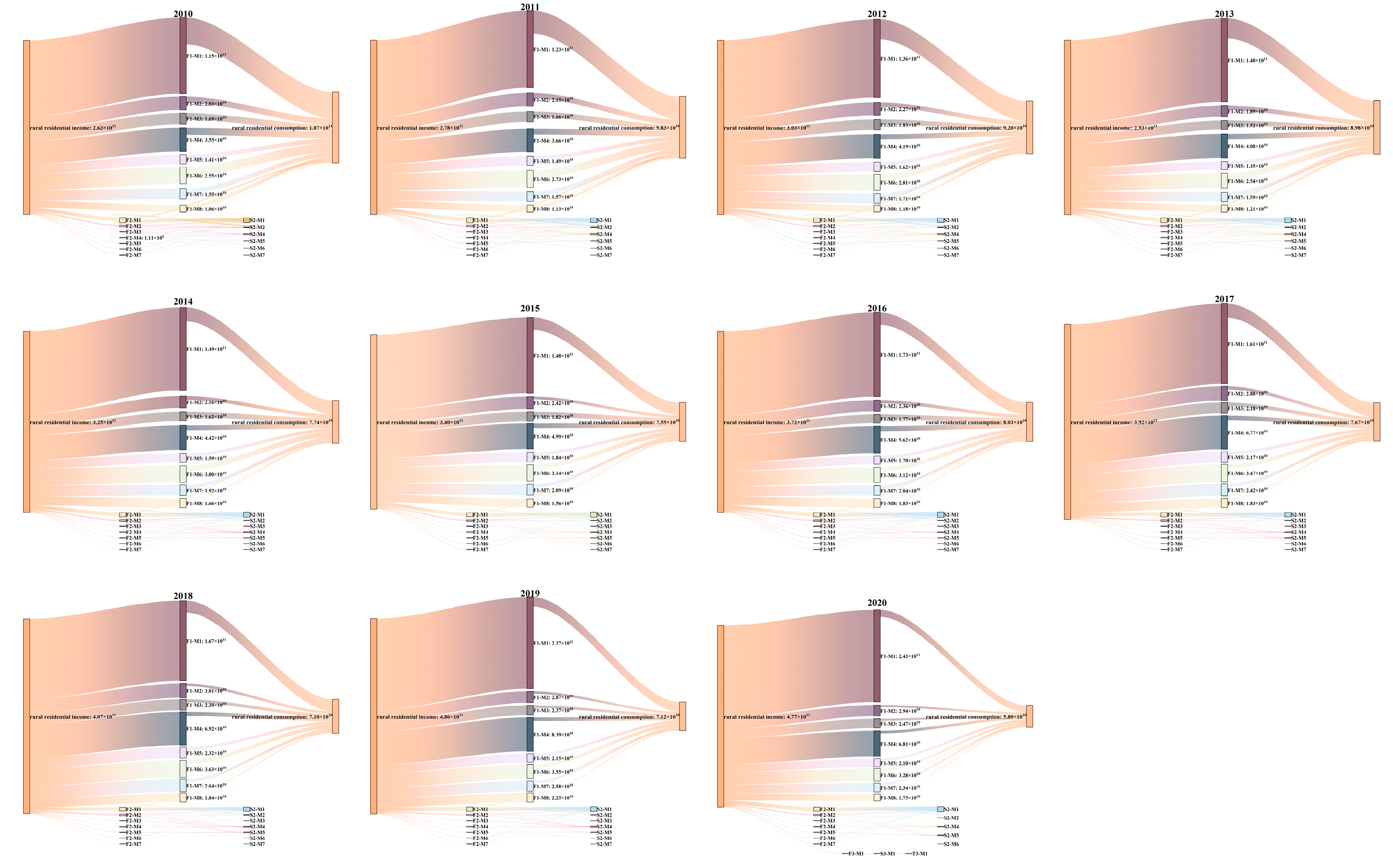
4.3. Path Analysis of Residential Water Consumption Structures
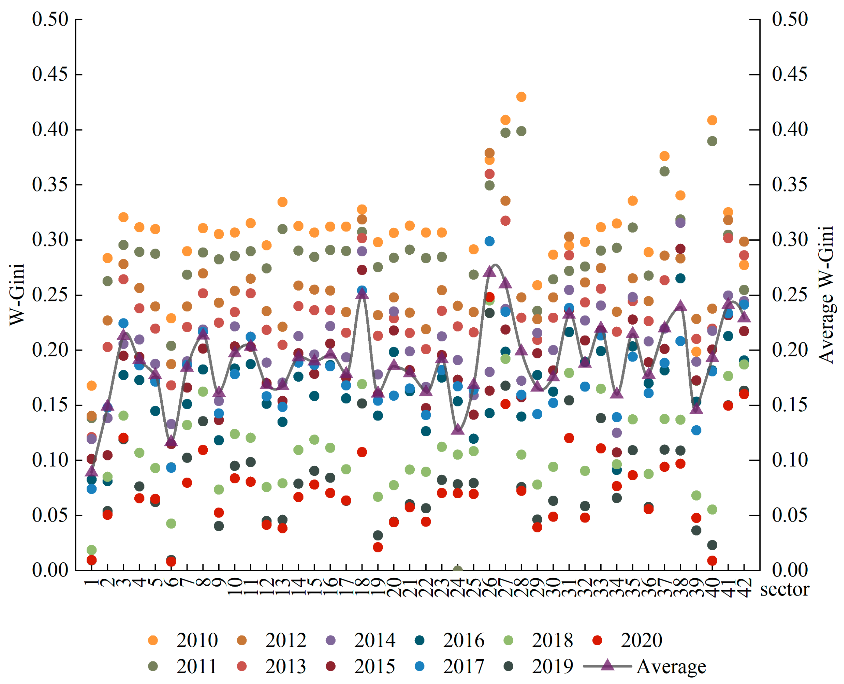
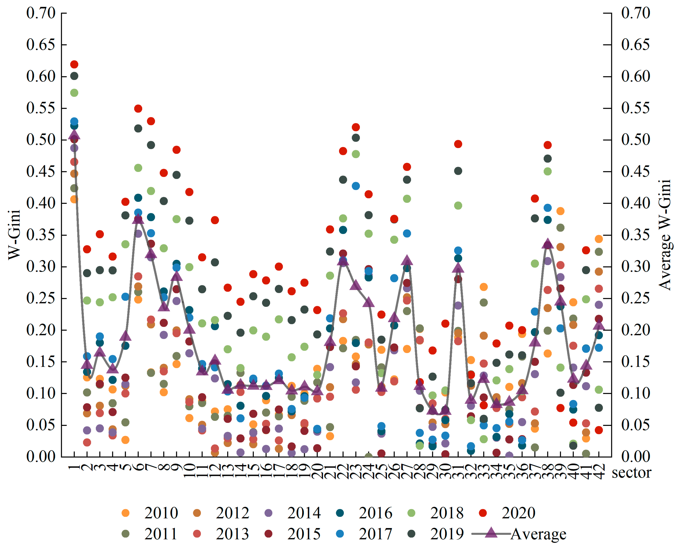
4.4. Inequity in Water Consumption Between Urban and Rural Populations
5. Conclusions and Policy Implications
5.1. Conclusions
5.2. Policy Recommendations
- (1)
- Adopt differentiated water management policies
- (2)
- Accelerate technological progress
- (3)
- Incentives for sustainable practices
- (4)
- Bridging the water divide
Author Contributions
Funding
Data Availability Statement
Conflicts of Interest
References
- Sun, S.; Zhou, X.; Liu, H.; Jiang, Y.; Zhou, H.; Zhang, C.; Fu, G. Unraveling the effect of inter-basin water transfer on reducing water scarcity and its inequality in China. Water Res. 2021, 194, 116931. [Google Scholar] [CrossRef] [PubMed]
- Ding, T.; Chen, J.; Fang, L.; Ji, J.; Fang, Z. Urban ecosystem services supply-demand assessment from the perspective of the water-energy-food nexus. Sustain. Cities Soc 2023, 90, 104401. [Google Scholar] [CrossRef]
- United Nations. Sustainable Development Goals Report 2018; United Nations: New York, NY, USA, 2018. [Google Scholar]
- Chen, S.; Song, Y.; Gao, P. Environmental, social, and governance (ESG) performance and financial outcomes: Analyzing the impact of ESG on financial performance. J. Environ. Manag. 2023, 345, 118829. [Google Scholar] [CrossRef] [PubMed]
- Han, Y.; Duan, H.; Du, X.; Jiang, L. Chinese household environmental footprint and its response to environmental awareness. Sci. Total Environ. 2021, 782, 146725. [Google Scholar] [CrossRef]
- Tu, C.; Mu, X.; Chen, J.; Kong, L.; Zhang, Z.; Lu, Y.; Hu, G. Study on the interactive relationship between urban residents’ expenditure and energy consumption of production sectors. Energy Policy 2021, 157, 112502. [Google Scholar] [CrossRef]
- Su, B.; Ang, B.W. Multiplicative structural decomposition analysis of aggregate embodied energy and emission intensities. Energy Econ. 2017, 65, 137–147. [Google Scholar] [CrossRef]
- Arce, R.d.; Mahía, R.o. Unbiasing the estimate of the role of income in carbon footprint of households: Analysis of the Spanish case as a pilot study. Heliyon 2023, 9, e16394. [Google Scholar] [CrossRef]
- Ekinci, E.; Mangla, S.K.; Kazancoglu, Y.; Sarma, P.; Sezer, M.D.; Ozbiltekin-Pala, M. Resilience and complexity measurement for energy efficient global supply chains in disruptive events. Technol. Forecast. Soc. Chang. 2022, 179, 121634. [Google Scholar] [CrossRef]
- Qin, P.; Chen, S.; Tan-Soo, J.; Zhang, X. Urban household water usage in adaptation to climate change: Evidence from China. Environ. Sci. Policy 2022, 136, 486–496. [Google Scholar] [CrossRef]
- Yang, M.; Zhang, X.; Zhang, Y.; Fath, B.D. Consistence of structural changes in food nitrogen consumption between rural and urban residents in the context of rapid urbanization. Ecol. Model. 2022, 471, 110057. [Google Scholar] [CrossRef]
- Barnett, M.J.; Smith, D.J.; Endter-Wada, J.; Haeffner, M. A multilevel analysis of the drivers of household water consumption in a semi-arid region. Sci. Total Environ. 2020, 712, 136489. [Google Scholar] [CrossRef] [PubMed]
- Chen, Z.; Song, Y.; Li, Y.; Li, Z. Assessing the contaminant reduction effects of the COVID-19 pandemic in China. J. Clean. Prod. 2023, 424, 138887. [Google Scholar] [CrossRef]
- Lin, B.; Teng, Y. Structural path and decomposition analysis of sectoral carbon emission changes in China. Energy 2022, 261, 125331. [Google Scholar] [CrossRef]
- Niu, C.; Wang, X.; Chang, J.; Wang, Y.; Guo, A.; Ye, X.; Wang, Q.; Li, Z. Integrated model for optimal scheduling and allocation of water resources considering fairness and efficiency: A case study of the Yellow River Basin. J. Hydrol. 2023, 626, 130236. [Google Scholar] [CrossRef]
- Shi, C.; Wu, C.; Zhang, J.; Zhang, C.; Xiao, Q. Impact of urban and rural food consumption on water demand in China—From the perspective of water footprint. Sustain. Prod. Consum. 2022, 34, 148–162. [Google Scholar] [CrossRef]
- Liao, X.; Chai, L.; Liang, Y. Income impacts on household consumption’s grey water footprint in China. Sci. Total Environ. 2021, 755, 142584. [Google Scholar] [CrossRef]
- Fan, J.; Wang, J.; Zhang, X.; Kong, L.; Song, Q. Exploring the changes and driving forces of water footprints in China from 2002 to 2012: A perspective of final demand. Sci. Total Environ. 2019, 650, 1101–1111. [Google Scholar] [CrossRef]
- Zhao, J.; Han, T.; Wang, C.; Shi, X.; Wang, K.; Zhao, M.; Chen, F.; Chu, Q. Assessing variation and driving factors of the county-scale water footprint for soybean production in China. Agric. Water Manag. 2022, 263, 107469. [Google Scholar] [CrossRef]
- Han, A.; Chai, L.; Liu, P. How much environmental burden does the shifting to nutritional diet bring? Evidence of dietary transformation in rural China. Environ. Sci. Policy 2023, 145, 129–138. [Google Scholar] [CrossRef]
- Li, D.; Zuo, Q.; Zhang, Z. A new assessment method of sustainable water resources utilization considering fairness-efficiency-security: A case study of 31 provinces and cities in China. Sustain. Cities Soc. 2022, 81, 103839. [Google Scholar] [CrossRef]
- Fu, Z.; Sun, S.; Fang, C. Unequal prefecture-level water footprints in China: The urban-rural divide. Sci. Total Environ. 2024, 912, 169089. [Google Scholar] [CrossRef] [PubMed]
- Zhang, P.; Zou, Z.; Liu, G.; Feng, C.; Liang, S.; Xu, M. Socioeconomic drivers of water use in China during 2002–2017. Resour. Conserv. Recycl. 2020, 154, 104636. [Google Scholar] [CrossRef]
- Aladejare, S.A. Economic prosperity, asymmetric natural resource income, and ecological demands in resource-reliant economies. Resour. Policy 2023, 82, 103435. [Google Scholar] [CrossRef]
- Li, J.; Huang, K.; Yu, Y.; Qu, S.; Xu, M. Telecoupling China’s city-level water withdrawal with distant consumption. Environ. Sci. Technol. 2023, 57, 4332–4341. [Google Scholar] [CrossRef]
- Fan, J.; Feng, X.; Dong, Y.; Zhang, X. A global comparison of carbon-water-food nexus based on dietary consumption. Glob. Environ. Chang. 2022, 73, 102489. [Google Scholar] [CrossRef]
- Mach, R.; Weinzettel, J.; Ščasný, M. Environmental impact of consumption by Czech households: Hybrid input–output analysis linked to household consumption data. Ecol. Econ. 2018, 149, 62–73. [Google Scholar] [CrossRef]
- Zhang, Z.; Zuo, Q.; Wu, Q.; Li, D.; Ma, J. Multisectoral water-carbon pressures and economic benefits in China: An embodied perspective driven by consumption. Sustain. Prod. Consum. 2024, 45, 42–56. [Google Scholar] [CrossRef]
- Du, M.; Liao, L.; Wang, B.; Chen, Z. Evaluating the effectiveness of the water-saving society construction in China: A quasi-natural experiment. J. Environ. Manag. 2021, 277, 111394. [Google Scholar] [CrossRef]
- Xu, W.; Xie, Y.; Ji, L.; Cai, Y.; Yang, Z.; Xia, D. Spatial-temporal evolution and driving forces of provincial carbon footprints in China: An integrated EE-MRIO and WA-SDA approach. Ecol. Eng. 2022, 176, 106543. [Google Scholar] [CrossRef]
- Yang, Y.; Liu, J.; Lin, Y.; Li, Q. The impact of urbanization on China’s residential energy consumption. Struct. Chang. Econ. Dyn. 2019, 49, 170–182. [Google Scholar] [CrossRef]
- Wang, M.; Feng, C. Decomposing the change in energy consumption in China’s nonferrous metal industry: An empirical analysis based on the LMDI method. Renew. Sustain. Energy Rev. 2018, 82, 2652–2663. [Google Scholar] [CrossRef]
- Mi, Z.; Meng, J.; Guan, D.; Shan, Y.; Liu, Z.; Wang, Y.; Feng, K.; Wei, Y.-M. Pattern changes in determinants of Chinese emissions. Environ. Res. Lett. 2017, 12, 074003. [Google Scholar] [CrossRef]
- Cai, B.; Jiang, L.; Liu, Y.; Wang, F.; Zhang, W.; Yan, X.; Ge, Z. Regional trends and socioeconomic drivers of energy-related water use in China from 2007 to 2017. Energy 2023, 275, 127404. [Google Scholar] [CrossRef]
- Cai, B.; Guo, M. Exploring the drivers of quantity- and quality-related water scarcity due to trade for each province in China. J. Environ. Manag. 2023, 333, 117423. [Google Scholar] [CrossRef]
- Owen, A.; Scott, K.; Barrett, J. Identifying critical supply chains and final products: An input–output approach to exploring the energy-water-food nexus. Appl. Energy 2018, 210, 632–642. [Google Scholar] [CrossRef]
- Liu, Y.; Song, Y. Does artificial ecosystem recharge make sense? based on the coupled water orbit research framework. Ecol. Indic. 2024, 166, 112496. [Google Scholar] [CrossRef]
- Zhao, G.; Gao, C.; Xie, R.; Lai, M.; Yang, L. Provincial water footprint in China and its critical path. Ecol. Indic. 2019, 105, 634–644. [Google Scholar] [CrossRef]
- Duarte, R.; Miranda-Buetas, S.; Sarasa, C. Household consumption patterns and income inequality in EU countries: Scenario analysis for a fair transition towards low-carbon economies. Energy Econ. 2021, 104, 105614. [Google Scholar] [CrossRef]
- Yang, Y.; Yang, H.; Cheng, Y. Why is it crucial to evaluate the fairness of natural capital consumption in urban agglomerations in terms of ecosystem services and economic contribution? Sustain. Cities Soc. 2021, 65, 102644. [Google Scholar] [CrossRef]
- Liu, G.; Zhang, F. Inequality of household water footprint consumption in China. J. Hydrol. 2022, 612, 128241. [Google Scholar] [CrossRef]
- Ma, S.; Xu, X.; Li, C.; Zhang, L.; Sun, M. Energy consumption inequality decrease with energy consumption increase: Evidence from rural China at micro scale. Energy Policy 2021, 159, 112638. [Google Scholar] [CrossRef]
- Matos, C.; Bentes, I.; Pereira, S.; Goncalves, A.M.; Faria, D.; Briga-Sa, A. Which are the factors that may explain the differences in water and energy consumptions in urban and rural environments? Sci. Total Environ. 2018, 642, 421–435. [Google Scholar] [CrossRef]
- Wang, F.; Xu, B.; Si, Y.; Shang, Y.; Zhang, W.; Cai, B.; Jiang, M.; Xu, S.; Lu, S. Components and drivers of household water footprint inequality in China. Sustain. Prod. Consum. 2023, 43, 1–14. [Google Scholar] [CrossRef]
- Liu, M.; Fang, C.; Bai, Y.; Sun, B.; Liao, X.; Liu, Z. Regional inequality and urban-rural difference of dietary water footprint in China. Resour. Conserv. Recycl. 2023, 199, 107236. [Google Scholar] [CrossRef]
- Cheng, X.; Wu, X.; Guan, C.; Sun, X.; Zhang, B. Impacts of production structure changes on global CH4 emissions: Evidences from income-based accounting and decomposition analysis. Ecol. Econ. 2023, 213, 107967. [Google Scholar] [CrossRef]
- Pang, Q.; Xiang, M.; Zhang, L.; Chiu, Y.-h. Indirect carbon emissions from household consumption of middle-income groups: Evidence from Yangtze River Economic Belt in China. Energy Sustain. Dev. 2023, 76, 101280. [Google Scholar] [CrossRef]
- Avelino, A.F.T.; Franco-Solís, A.; Carrascal-Incera, A. Revisiting the temporal Leontief inverse: New insights on the analysis of regional technological economic change. Struct. Change Econ. Dyn. 2021, 59, 79–89. [Google Scholar] [CrossRef]
- Li, Y.; Su, B.; Dasgupta, S. Structural path analysis of India’s carbon emissions using input–output and social accounting matrix frameworks. Energy Econ. 2018, 76, 457–469. [Google Scholar] [CrossRef]
- Zhang, B.; Qu, X.; Meng, J.; Sun, X. Identifying primary energy requirements in structural path analysis: A case study of China 2012. Appl. Energy 2017, 191, 425–435. [Google Scholar] [CrossRef]
- Castaño, A.; Lufin, M.; Atienza, M. A structural path analysis of Chilean mining linkages between 1995 and 2011. What are the channels through which extractive activity affects the economy? Resour. Policy 2019, 60, 106–117. [Google Scholar] [CrossRef]
- Wang, Q.; Wang, X. Does economic growth help reduce inequality of water consumption? Insight from evolution and drivers of inequality in water consumption in China. Environ. Sci. Pollut. Res. 2021, 28, 37338–37353. [Google Scholar] [CrossRef] [PubMed]
- Sun, C.; Zhang, Y.; Peng, S.; Zhang, W. The inequalities of public utility products in China: From the perspective of the Atkinson index. Renew. Sust. Energ. Rev. 2015, 51, 751–760. [Google Scholar] [CrossRef]
- Dai, C.; Qin, X.; Chen, Y.; Guo, H. Dealing with equality and benefit for water allocation in a lake watershed: A Gini-coefficient based stochastic optimization approach. J. Hydrol. 2018, 561, 322–334. [Google Scholar] [CrossRef]
- Ministry of Water Resources. Water Resources Bulletin; China Water and Power Press: Beijing, China, 2010.
- Ministry of Water Resources. Water Resources Bulletin; China Water and Power Press: Beijing, China, 2011.
- Ministry of Water Resources. Water Resources Bulletin; China Water and Power Press: Beijing, China, 2012.
- Ministry of Water Resources. Water Resources Bulletin; China Water and Power Press: Beijing, China, 2013.
- Ministry of Water Resources. Water Resources Bulletin; China Water and Power Press: Beijing, China, 2014.
- Ministry of Water Resources. Water Resources Bulletin; China Water and Power Press: Beijing, China, 2015.
- Ministry of Water Resources. Water Resources Bulletin; China Water and Power Press: Beijing, China, 2016.
- Ministry of Water Resources. Water Resources Bulletin; China Water and Power Press: Beijing, China, 2017.
- Ministry of Water Resources. Water Resources Bulletin; China Water and Power Press: Beijing, China, 2018.
- Ministry of Water Resources. Water Resources Bulletin; China Water and Power Press: Beijing, China, 2019.
- Ministry of Water Resources. Water Resources Bulletin; China Water and Power Press: Beijing, China, 2020.
- Lu, Y.; Wang, J.; Liu, J.; Qin, F.; Wang, J. Evaluating water withdrawals for regional water management under a data-driven framework. Chin. Geogr. Sci. 2022, 32, 521–536. [Google Scholar] [CrossRef]
- Wang, X.; Huang, K.; Yu, Y.; Hu, T.; Xu, Y. An input–output structural decomposition analysis of changes in sectoral water footprint in China. Ecol. Indic. 2016, 69, 26–34. [Google Scholar] [CrossRef]
- Zhang, C.; Anadon, L.D. A multi-regional input–output analysis of domestic virtual water trade and provincial water footprint in China. Ecol. Econ. 2014, 100, 159–172. [Google Scholar] [CrossRef]
- Peng, S.; Wang, X.; Du, Q.; Wu, K.; Lv, T.; Tang, Z.; Wei, L.; Xue, J.; Wang, Z. Evolution of household carbon emissions and their drivers from both income and consumption perspectives in China during 2010-2017. J. Environ. Manag. 2023, 326, 116624. [Google Scholar] [CrossRef]
- Zheng, L.; Zou, H.; Duan, X.; Lin, Z.; Du, H. Potential determinants affecting the growth of China’s ocean economy: An input–output structural decomposition analysis. Mar. Policy 2023, 150, 105520. [Google Scholar] [CrossRef]
- Wang, C.; Zhan, J.; Li, Z.; Zhang, F.; Zhang, Y. Structural decomposition analysis of carbon emissions from residential consumption in the Beijing-Tianjin-Hebei region, China. J. Clean. Prod. 2019, 208, 1357–1364. [Google Scholar] [CrossRef]
- NBS. China Statistical Yearbook; China Statistics Press, China National Bureau of Statistics: Beijing, China, 2011.
- NBS. China Statistical Yearbook; China Statistics Press, China National Bureau of Statistics: Beijing, China, 2012.
- NBS. China Statistical Yearbook; China Statistics Press, China National Bureau of Statistics: Beijing, China, 2013.
- NBS. China Statistical Yearbook; China Statistics Press, China National Bureau of Statistics: Beijing, China, 2014.
- NBS. China Statistical Yearbook; China Statistics Press, China National Bureau of Statistics: Beijing, China, 2015.
- NBS. China Statistical Yearbook; China Statistics Press, China National Bureau of Statistics: Beijing, China, 2016.
- NBS. China Statistical Yearbook; China Statistics Press, China National Bureau of Statistics: Beijing, China, 2017.
- NBS. China Statistical Yearbook; China Statistics Press, China National Bureau of Statistics: Beijing, China, 2018.
- NBS. China Statistical Yearbook; China Statistics Press, China National Bureau of Statistics: Beijing, China, 2019.
- NBS. China Statistical Yearbook; China Statistics Press, China National Bureau of Statistics: Beijing, China, 2020.
- NBS. China Statistical Yearbook; China Statistics Press, China National Bureau of Statistics: Beijing, China, 2021.
- Lei, M.; Ding, Q.; Cai, W.; Wang, C. The exploration of joint carbon mitigation actions between demand- and supply-side for specific household consumption behaviors—A case study in China. Appl. Energy 2022, 324, 119740. [Google Scholar] [CrossRef]
- Geng, Y.; Cao, G.; Wang, L.; Wang, M.; Huang, J. Can drip irrigation under mulch be replaced with shallow-buried drip irrigation in spring maize production systems in semiarid areas of northern China? J. Sci. Food Agric. 2021, 101, 1926–1934. [Google Scholar] [CrossRef] [PubMed]
- Ye, W.; Ma, E.; Liao, L.; Hui, Y.; Liang, S.; Ji, Y.; Yu, S. Applicability of photovoltaic panel rainwater harvesting system in improving water-energy-food nexus performance in semi-arid areas. Sci. Total Environ. 2023, 896, 164938. [Google Scholar] [CrossRef] [PubMed]
- Qi, Z.; Song, J.; Yang, W.; Duan, H.; Liu, X. Revealing contributions to sulfur dioxide emissions in China: From the dimensions of final demand, driving effect and supply chain. Resour. Conserv. Recycl. 2020, 160, 104864. [Google Scholar] [CrossRef]
- Hao, P.; Tang, S. Migration and consumption among poor rural households in China. Habitat. Int. 2023, 137, 102832. [Google Scholar] [CrossRef]
- Ma, W.; Vatsa, P.; Zheng, H.; Rahut, D.B. Nonfarm employment and consumption diversification in rural China. Econ. Anal. Policy 2022, 76, 582–598. [Google Scholar] [CrossRef]
- Tan, T.; Wu, L.; Deng, Z.; Dawood, M.; Yu, Y.; Wang, Z.; Huang, K. The urban-rural dietary water footprint and its inequality in China’s urban agglomerations. Sci. Total Environ. 2024, 953, 176045. [Google Scholar] [CrossRef]
- Huang, L.; Long, Y.; Chen, J.; Yoshida, Y. Sustainable lifestyle: Urban household carbon footprint accounting and policy implications for lifestyle-based decarbonization. Energy Policy 2023, 181, 113696. [Google Scholar] [CrossRef]


| Number | Sector | Consumption Categories |
|---|---|---|
| S1 | Agriculture | M1 |
| S2 | Mining and washing of coal | M4 |
| S3 | Extraction of petroleum and natural gas | M4 |
| S4 | Mining and processing of metal ores | M4 |
| S5 | Mining and processing of nonmetal and other ores | M4 |
| S6 | Food and tobacco processing | M1 |
| S7 | Textile industry | M2 |
| S8 | Manufacture of leather, fur, feather and related products | M2 |
| S9 | Processing of timber and furniture | M4 |
| S10 | Manufacture of paper, printing and articles for culture, education and sport activity | M6 |
| S11 | Petroleum processing, coking and nuclear fuel processing | M5 |
| S12 | Manufacture of chemical products | M4, M6 |
| S13 | Manufacture of non-metallic mineral products | M3, M4 |
| S14 | Smelting and processing of metals | M4 |
| S15 | Manufacture of metal products | M3, M4 |
| S16 | Manufacture of general-purpose machinery | M1, M2, M7 |
| S17 | Manufacture of special-purpose machinery | M1, M2, M7 |
| S18 | Manufacture of transport equipment | M5 |
| S19 | Manufacture of electrical machinery and equipment | M4, M5, M6 |
| S20 | Manufacture of communication equipment, computers and other electronic equipment | M5 |
| S21 | Manufacture of measuring instruments | M4, M6 |
| S22 | Other manufacturing and waste resources | M3, M4, M6, M7, M8 |
| S23 | Waste products and materials | \ |
| S24 | Repair of metal products, machinery and equipment | M3, M4 |
| S25 | Production and distribution of electric power and heat power | M3 |
| S26 | Production and distribution of gas | M3 |
| S27 | Production and distribution of tap water | M3 |
| S28 | Construction | M3 |
| S29 | Wholesale and retail trades | M1, M2, M3, M4, M5, M6, M7, M8 |
| S30 | Transport, storage and postal services | M5 |
| S31 | Accommodation and catering | M1, M6 |
| S32 | Information transfer, software and information technology services | M5, M6 |
| S33 | Finance | M7 |
| S34 | Real estate | M3 |
| S35 | Leasing and commercial services | M5, M6 |
| S36 | Scientific research and polytechnic services | M6, M8 |
| S37 | Administration of water, environment and public facilities | M3, M6 |
| S38 | Resident, repair and other services | M4, M8 |
| S39 | Education | M6 |
| S40 | Health care and social work | M7 |
| S41 | Culture, sports and entertainment | M6, M7 |
| S42 | Public administration, social insurance and social organizations | M7 |
Disclaimer/Publisher’s Note: The statements, opinions and data contained in all publications are solely those of the individual author(s) and contributor(s) and not of MDPI and/or the editor(s). MDPI and/or the editor(s) disclaim responsibility for any injury to people or property resulting from any ideas, methods, instructions or products referred to in the content. |
© 2024 by the authors. Licensee MDPI, Basel, Switzerland. This article is an open access article distributed under the terms and conditions of the Creative Commons Attribution (CC BY) license (https://creativecommons.org/licenses/by/4.0/).
Share and Cite
Lv, T.; Song, Y.; Chen, Z. China’s Inequality in Urban and Rural Residential Water Consumption—A New Multi-Analysis System. Water 2025, 17, 37. https://doi.org/10.3390/w17010037
Lv T, Song Y, Chen Z. China’s Inequality in Urban and Rural Residential Water Consumption—A New Multi-Analysis System. Water. 2025; 17(1):37. https://doi.org/10.3390/w17010037
Chicago/Turabian StyleLv, Tongtong, Yu Song, and Zuxu Chen. 2025. "China’s Inequality in Urban and Rural Residential Water Consumption—A New Multi-Analysis System" Water 17, no. 1: 37. https://doi.org/10.3390/w17010037
APA StyleLv, T., Song, Y., & Chen, Z. (2025). China’s Inequality in Urban and Rural Residential Water Consumption—A New Multi-Analysis System. Water, 17(1), 37. https://doi.org/10.3390/w17010037