Response of Soil Detachment Capacity to Hydrodynamic Characteristics Under Different Slope Gradients

Abstract

The mechanism of soil detachment on steep slopes is obviously different from that on gentle slopes. However, the slope effect of soil detachment remains unclear. The objective of this study was to quantify the slope effect of soil detachment capacity at the varying hydrodynamic characteristics. In this study, the soil detachment capacity (Dc) on clay loam and hydrodynamic characteristics were measured by conducting the runoff scouring experiments at 10 slope gradients (1.7–57.7%) and 5 unit flow discharges (0.022–0.089 m²·min⁻¹). The results showed that the relationships between Dc and hydrodynamic parameters were affected by slope gradient. Based on the optimal functional relationship, the hydrodynamic characteristics (flow velocity, flow shear stress, stream power, unit stream power, and unit energy) calculated by maximum and minimum Dc in this study changed by 19.91–95138.10%, and the Dc calculated by the maximum and minimum hydrodynamic characteristics could differ by up to nine orders of magnitude. Overall, the power function of hydrodynamic parameters was superior to the linear function in different slope gradients. The stream power was the best predictor for Dc compared with other hydrodynamic parameters. For all combinations of slope gradients, the adjusted coefficient of determination (Adj. R²) of the power relationship between Dc and stream power was 9.41–27.40% higher than it was between Dc and other hydrodynamic parameters. The coefficient and index of power function for different hydrodynamic parameters showed a trend change with increasing slope gradient, indicating that there was a slope effect on Dc. Further analysis found that Dc could be well predicted using a power combination equation of slope gradient, flow velocity, and flow depth (Adj. R² = 0.96). This study helps to better understand the mechanism of soil detachment and emphasizes that the slope effect should be considered when establishing a soil detachment equation.

1. Introduction

Soil erosion processes are controlled by both soil detachment capacity and sediment transport capacity [1,2,3]. Soil detachment is the sub-process of soil erosion and plays an important role in developing a physically based soil erosion model [4,5,6,7]. Accurately quantifying soil detachment capacity (Dc) is a key component in analyzing the sediment discharge at the exit sections of hillslope for the physically based soil erosion models, such as the Water Erosion Prediction Project (WEPP) [4], the European Soil Erosion Model (EUROSEM) [5], the Griffith University Erosion System Template (GUEST) [7], and the Digital Yellow River Integrated Model (DYRIM) [8]. However, the different hydrodynamic parameters (i.e., flow shear stress, stream power, and unit stream power) were applied to the above models in estimating the Dc. The characteristics of shallow overland flow and the mechanism of soil detachment on gentle slopes are obviously different from those on steep slopes [9,10]. Hence, it is very important to understand the dynamic mechanism of soil detachment from gentle to steep slopes for developing a physically based soil erosion model.

Soil property, slope gradient, and hydrodynamic characteristics are key factors influencing Dc [10,11,12]. The Dc is defined as the maximum rate at which the overland flow can detach soil at a sediment load of zero [2,13]. The soil detachability depends on the soil property [6]. The hydrodynamic characteristic is affected by the conditions of the slope gradient and flow discharge [14]. The relationships between Dc and hydrodynamic parameters have been extensively studied. However, there are different opinions regarding the form of the soil detachment capacity equation and the optimum predictor of it. Previous studies indicated that the flow shear stress is the best predictor of Dc, which is adopted by the WEPP for the widely used physically based soil erosion model in the world [4,15]. For EUROSEM, the unit stream power is adopted to calculate Dc [5]. Parhizkar et al. [16] also illustrated that the Dc can be well predicted by unit stream power. Most studies indicated that the stream power is an optimal hydrodynamic parameter in calculating Dc [11,14,17,18], which is adopted by the models of GUEST and DYRIM [7,8]. Moreover, different forms of Dc equations have been found in previous studies, including linear function [14,19,20], logarithmic function [21], power function [16,18], etc. The above results illustrated that existing research on Dc remains controversial.

Early studies on soil detachment mainly focused on gentle slopes of <17.6% [13,22,23], with representative research results such as WEPP and EUROSEM [4,5]. However, there is an obvious difference between steep slopes and gentle slopes [2,9,18]. More and more researchers have begun to focus on the development of Dc on steep slopes, with representative research results such as DYRIM [8]. Liu et al. [24] and Wang et al. [2] indicated that the soil erosion model developed on gentle slopes is not suitable for steep slopes. Severe soil erosion on steep slopes of >17.6% usually occurs, resulting in hyper-concentrated flow on the Loess Plateau of China [25,26]. Numerous studies have been conducted to investigate the relationships between Dc and hydrodynamic parameters on steep slopes [11,15,20,27]. However, it is still unclear why the equation of Dc on gentle slopes cannot be extended to steep slopes. Whether there is a slope effect on Dc needs further study. Therefore, it is necessary to better understand the dynamic mechanism of Dc in different slope gradients from gentle to steep using more controlled experiments.

Previous studies have made a substantial contribution to the understanding and quantification of Dc in different conditions of soil types and hydrodynamic characteristics. However, the effects of hydrodynamic characteristics on Dc by shallow overland flow are not fully understood in different slope gradients. The objectives of this study were to (1) establish the relationships between Dc and different hydrodynamic parameters in different slope gradients; (2) identify the best hydrodynamic parameter and form in calculating Dc; and (3) quantify the slope effect of Dc at the varying hydrodynamic characteristics.

2. Materials and Methods

2.1. Experimental Devices and Designs

The overland flow scouring experiment was conducted on the clay loam soil (USDA fraction classification criteria). The test soil sample was collected from the surface soil layer (0–20 cm) in Yangling of Shanxi Province in China. The test sample is the main cultivated soil in Guanzhong Plain of the southern Loess Plateau. The collected soil samples were thoroughly mixed to eliminate the effects of variability. The soil has 28.20% clay, 41.60% silt, 30.20% sand, and 21.26 g·kg⁻¹ soil organic matter content [12]. The soil was air dried and sieved through a 10-mm sieve, which was packed into a cutting ring with a bulk density of 1.15 g·cm⁻³. The cutting ring dimension was 7 cm in diameter and 5 cm in depth. There was a soil sample container at 150 cm from the outlet of the scouring flume that was just large enough to fit the cutting ring. The surface of the soil sample container with the cutting ring was parallel to the scouring flume bed. The scouring flume was 4 m long, 0.3 m wide, and 0.2 m deep and was used to measure Dc in a smooth flume bed. The flume was made of organic glass, and slope gradient could be adjusted by up to 57.7% using a slope-adjustment device. There was a steady flow trough at the top of the scouring flume and it was connected to a flow control valve and glass rotor flowmeter (LZB-40, SKJYLEAN, Suzhou, China). A grid-shaped flow stabilizing plate was installed in the steady flow trough to maintain the stability of the experimental inflow water. The error of the glass rotor flowmeter is less than 2.5%. In order to reveal the difference in Dc between gentle slopes and steep slopes, ten slope gradients (1.7%, 5.2%, 8.7%, 12.3%, 17.6%, 21.3%, 26.8%, 36.4%, 46.6%, and 57.7%) and five unit width flow discharges (0.022, 0.039, 0.056, 0.072, and 0.089 m²·min⁻¹) were designed in this study according to the slope distribution and runoff characteristics under natural conditions. The experiment for each combination of unit width flow discharge and slope gradient was repeated three times using the different soil samples.

2.2. Experimental Methods

Prior to the experiment, the cutting rings containing the soil sample were saturated by wetting for 12 h. The unit width flow discharge and slope gradient were adjusted to the design requirements. The soil sample in the cutting ring was placed in a soil sample container of scouring flume. The Dc was measured after the flow discharge reached stability and the time was recorded using a stopwatch. The test stopped when the soil depth was 1.5 cm to reduce the effect of the side-wall of the cutting ring [11], and the maximum duration of each test was 300 s before this limit for lower flow discharges and gentler slopes [27]. The scoured soil sample was oven-dried and weighed to calculate Dc after the experiment.

2.3. Hydrodynamic Characteristics Measurement

The flow depth was measured 9 times at three cross sections using a level probe (accuracy of 0.01 cm), located at 0.2 m and 1 m from the soil sample container of scouring flume. The mean flow depth was obtained by calculating the 9 measured values of flow depth. The mean flow velocity (v, m·s⁻¹) was calculated by the continuum equation as follows:

$$v={\displaystyle \frac{Q}{BH}}$$

(1)

where Q is the flow discharge (m³·s⁻¹), B is the width of the scouring flume (m), and H is the mean flow depth (m). The flow shear stress (τ, Pa), stream power (ω, N·m⁻¹·s⁻¹), unit stream power (Us, m·s⁻¹), and unit energy (E, m) were defined as [14,28,29,30].

$$\tau =\gamma RJ$$

(2)

$$\omega =\tau v$$

(3)

$$Us=vJ$$

(4)

$$E={{\displaystyle \frac{av}{2g}}}^2+H\cos \theta$$

(5)

where γ is the water specific weight (N·m⁻³), R is the hydraulic radius (m), J is the hydraulic gradient (sinθ, θ is the slope angle (°)), and a is the kinetic energy correction coefficient (approximated as 1).

2.4. Data Analysis

A Pearson correlation matrix was used to analyze the correlations between slope gradient (S), Q, h, v, τ, ω, Us, E, and Dc with a significance level of p < 0.05 using IBM SPSS Statistics 22.0 (IBM Corp., Armonk, NY, USA). The linear and nonlinear fitting methods were used to quantify the relationship between D_c and hydrodynamic parameters using the 1stOpt 1.5 software (7D-Soft High Technology Inc., Beijing, China). The prediction accuracy of the regression equation was evaluated using the adjusted coefficient of determination (Adj. R²) [31,32].

3. Results

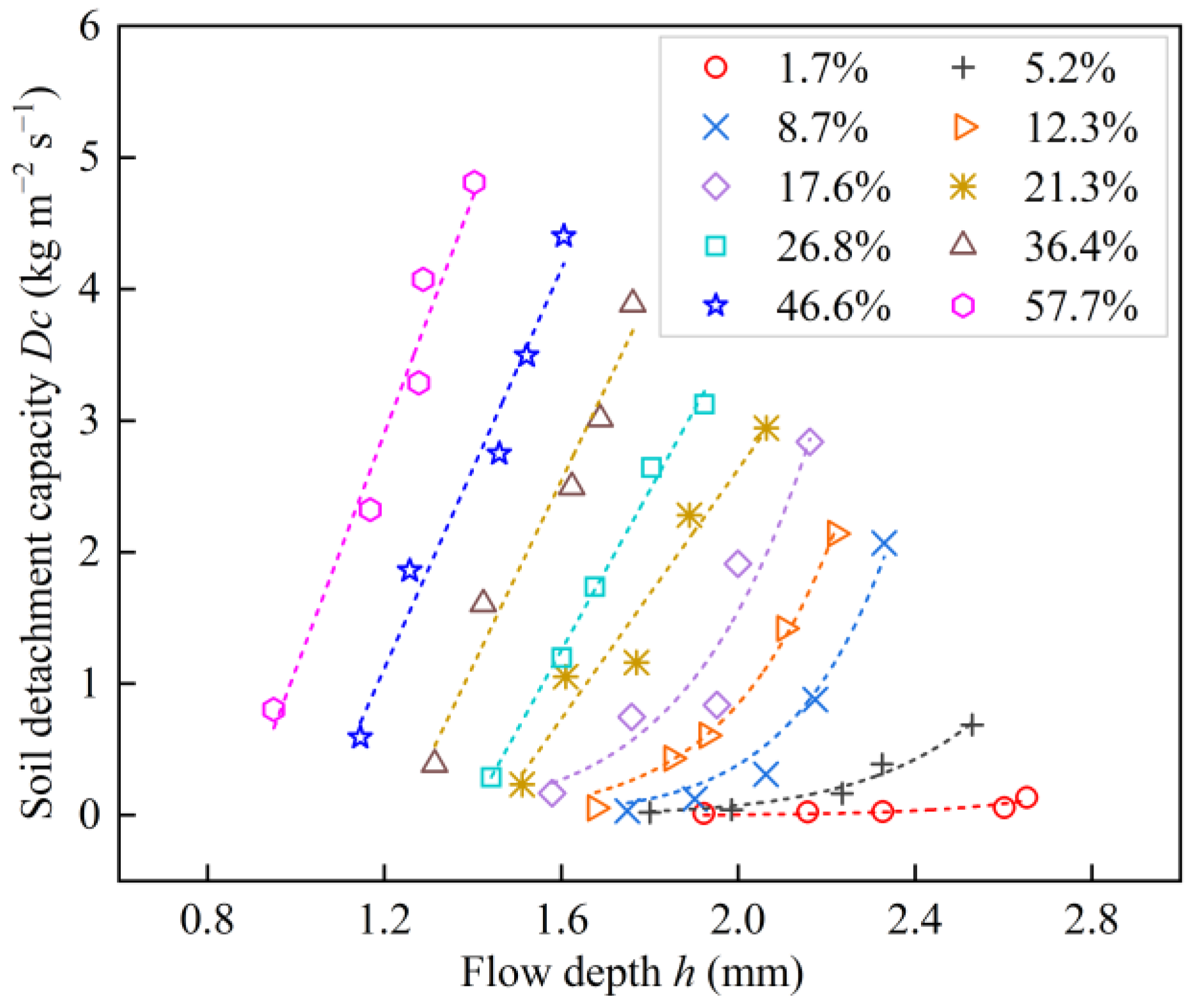
3.1. The Effect of Hydrodynamic Characteristics on the Soil Detachment Capacity

Significant differences between Dc and hydrodynamic characteristics were shown in Figure 1. Dc showed a significantly positive correlation with hydrodynamic parameters at the significance level of 0.01, and the ranking of the correlation coefficient was stream power > flow velocity = unit energy > unit stream power > flow shear stress > slope gradient > flow discharge. Conversely, the Pearson correlation analysis showed a significantly negative correlation between Dc and flow depth (p < 0.05) in Figure 1. This is because the steeper the slope, the shallower the flow depth (Figure 2). Actually, the Dc increased with flow depth for a given slope gradient (Figure 2). The relationships between Dc and flow depth shifted from power functions for slope gradient of ≤17.6% (Adj. R² ≥ 0.80, p < 0.030) to linear functions for a slope gradient of ≥21.3% (

Table 1. Relationship between soil detachment capacity and flow depth in different slope gradients.

Slope Gradient %	Power Function Dc = a1 h b1				Linear Function Dc = k1 (h–hc)
	a1	b1	Adj. R2	p	k1	vc	Adj. R2	p
1.7	0.0000010	11.91	0.80	0.025	0.13	2.00	0.53	0.10
5.2	0.00010	9.54	0.96	<0.010	0.90	1.89	0.80	0.025
8.7	0.00023	10.69	0.97	<0.010	3.33	1.84	0.74	0.039
12.3	0.0016	9.05	0.99	<0.010	3.85	1.71	0.93	<0.010
17.6	0.0068	7.84	0.89	<0.010	4.33	1.59	0.79	0.029
21.3	0.07	5.30	0.89	<0.010	4.75	1.45	0.93	<0.010
26.8	0.09	5.49	0.92	<0.010	6.09	1.39	0.99	<0.010
36.4	0.18	5.43	0.94	<0.010	7.05	1.24	0.96	<0.010
46.6	0.52	4.53	0.95	<0.010	7.59	1.05	0.96	<0.010
57.7	1.27	4.05	0.94	<0.010	8.96	0.88	0.95	<0.010

Note: Dc is the soil detachment capacity (kg·m⁻²·s⁻¹); h is the flow depth (mm); a₁ and b₁ are the coefficient and index of power function, respectively; k₁ is the coefficient of linear function; h_c is the critical flow depth (mm).

). As shown in Table 1, the Adj. R² of the power function was 6.45–50.94% higher that of the linear function for slope gradient of ≤17.6% and that of the linear function was 1.05–7.61% higher that of the power function for a slope gradient of ≥21.3%. Based on the power function equations for gentler slopes of ≤17.6% and linear function equations for steeper slopes of ≥21.3% in Table 1, the flow depth calculated by the maximum Dc of 4.81 kg·s⁻¹·m⁻² in this study decreased from 3.6 to 1.4 mm (61.11%) with increasing slope gradient, and it was calculated by the minimum Dc of 0.011 kg·s⁻¹·m⁻² that decreased from 2.2 to 0.9 mm (59.10%) in different slope gradients. The Dc calculated by the maximum flow depth of 2.7 mm changed from 0.11 to 15.88 kg·s⁻¹·m⁻² (143.36%) in different slope gradients. The Dc calculated by the minimum flow depth condition had a difference of six orders of magnitude except for the slopes of 21.3% to 46.6%.

The flow depth and velocity are basic parameters in calculating hydrodynamic characteristics, such as flow shear stress, stream power, unit stream power, and unit energy. The relationships between Dc and flow velocity are shown in Figure 3 and

Table 2. Relationship between soil detachment capacity and flow velocity in different slope gradients.

Slope Gradient %	Power Function Dc = a2 v b2				Linear Function Dc = k2 (v–vc)
	a2	b2	Adj. R2	p	k1	vc	Adj. R2	p
1.7	5.59	4.26	0.94	<0.010	0.31	0.22	0.67	0.057
5.2	7.16	4.39	0.99	<0.010	1.70	0.26	0.80	0.027
8.7	7.42	3.32	0.88	0.011	3.96	0.26	0.83	<0.010
12.3	8.11	3.20	0.97	<0.010	4.50	0.25	0.86	0.014
17.6	6.97	2.52	0.96	<0.010	5.66	0.24	0.88	0.011
21.3	6.13	2.24	0.96	<0.010	5.52	0.23	0.91	<0.010
26.8	5.04	1.73	0.98	<0.010	5.67	0.22	0.99	<0.010
36.4	5.17	1.53	0.96	<0.010	6.12	0.20	0.98	<0.010
46.6	5.07	1.55	0.98	<0.010	5.99	0.20	0.99	<0.010
57.7	4.56	1.34	0.94	<0.010	5.59	0.20	0.96	<0.010
1.7–57.7	5.08	2.08	0.85	<0.010	6.08	0.27	0.84	<0.010

Note: Dc is the soil detachment capacity (kg·m⁻²·s⁻¹); v is the flow velocity (m·s⁻¹); a₂ and b₂ are the coefficient and index of power function, respectively; k₂ is the coefficient of linear function; v_c is the critical flow velocity (m·s⁻¹).

. The slope effect of Dc was also found in Figure 3a. The Adj. R² of the power function was 5.49% to 40.30% higher than that of the linear function for a slope gradient of ≤21.3%, and it was only 1.01% to 2.08% lower than that of the linear function for a slope gradient of >21.3% (Table 2). Overall, the power function relationship (Adj. R² > 0.84) was superior to the linear function relationship (Adj. R² > 0.66) in different slope gradients. However, the regression analysis for all combinations of slope gradients showed that there was a basically consistent performance for the power function (R² = 0.85) and linear function (R² = 0.84) in the simulating Dc (Figure 3b). Based on the power function equations in Table 2, the flow velocity calculated by the maximum Dc of 4.81 kg·s⁻¹·m⁻² changed from 0.85 to 1.04 m·s⁻¹ (22.35%) in different slope gradients and is calculated by the minimum Dc of 0.011 kg·s⁻¹·m⁻² that decreased from 0.23 to 0.011 m·s⁻¹ (95.22%) with an increasing slope gradient. Moreover, the Dc calculated by the maximum flow velocity of 1.06 m·s⁻¹ changed from 4.90 to 9.63 kg·s⁻¹·m⁻² (96.53%) in different slope gradients and is calculated by the minimum flow velocity of 0.19 m·s⁻¹ that increased from 0.0050 to 0.50 kg·s⁻¹·m⁻² (9900.00%) with an increasing slope gradient, which showed a difference of two orders of magnitude.

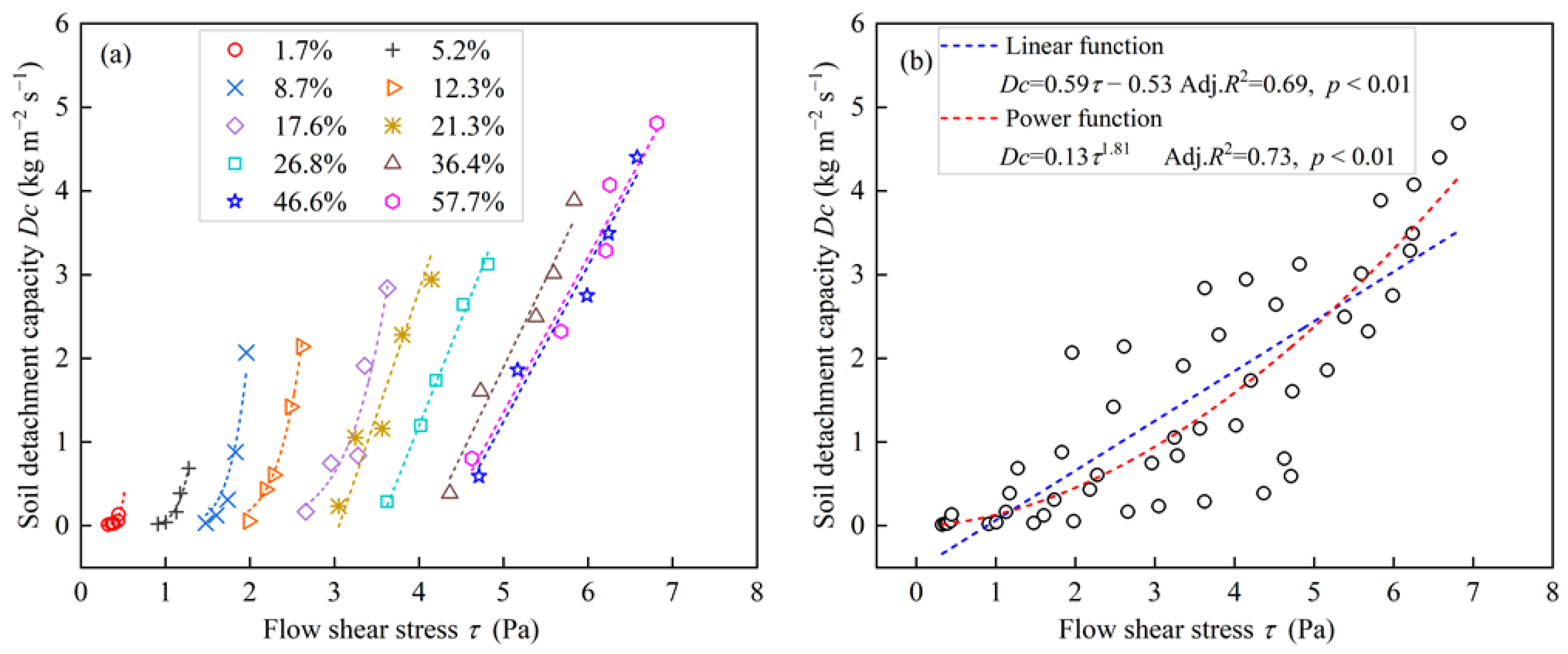
3.2. The Effect of Flow Shear Stress on the Soil Detachment Capacity

The relationships between Dc and flow shear stress are shown in

Table 3. Relationship between soil detachment capacity and flow shear stress in different slope gradients.

Slope Gradient %	Power Function Dc = a3 τ b3				Linear Function Dc = k3 (τ–τc)
	a3	b3	Adj. R2	p	k3	τc	Adj. R2	p
1.7	210.44	9.40	0.72	0.028	0.80	0.33	0.53	0.099
5.2	0.066	9.68	0.96	<0.010	1.81	0.96	0.80	0.026
8.7	0.0031	9.51	0.92	<0.010	2.10	1.39	0.74	0.018
12.3	0.00032	9.17	0.99	<0.010	2.40	1.91	0.94	<0.010
17.6	0.00010	7.94	0.89	<0.010	2.61	2.67	0.84	0.029
21.3	0.00039	6.36	0.86	<0.010	2.97	3.05	0.96	<0.010
26.8	0.00054	5.55	0.92	<0.010	2.54	3.53	0.99	<0.010
36.4	0.00057	4.99	0.94	<0.010	2.10	4.10	0.99	<0.010
46.6	0.00080	4.57	0.95	<0.010	1.87	4.32	0.96	<0.010
57.7	0.0020	4.08	0.95	<0.010	1.86	4.26	0.95	<0.010
1.7–57.7	0.13	1.81	0.73	<0.010	0.59	0.90	0.69	<0.010

Note: Dc is the soil detachment capacity (kg·m⁻²·s⁻¹); τ is the flow shear stress (Pa); a₃ and b₃ are the coefficient and index of power function, respectively; k₃ is the coefficient of linear function; τ_c is the critical flow shear stress (Pa).

. The Adj. R² of the power function was 5.32% to 35.85% higher than that of a linear function in 1.7–17.6% slopes. However, it was 1.04% to 10.42% lower than that of a linear function in 21.3–46.6% slopes. The relationship between Dc and flow shear stress shifted from power functions to linear functions with increasing slope gradients (Figure 4a). This result was consistent with that of flow depth. An interesting phenomenon is that the obvious slope effect for the relationship between Dc and flow shear stress was found in this study (Figure 4). We also found that the power function (Adj. R² = 0.73, p < 0.01) for all combinations of slope gradients was 5.80% higher than the linear function (Adj. R² = 0.69, p < 0.01) (Figure 4b). The performance of flow shear stress under all combinations of slope gradients was 15.12% to 26.26% lower than that under different slope gradients. Based on the power function equations for gentler slopes of ≤17.6% and linear function equations for steeper slopes of ≥21.3% in Table 3, the flow shear stress calculated by the maximum Dc of 4.81 kg·s⁻¹·m⁻² increased from 0.67 to 6.89 Pa (928.36%) with increasing slope gradient and is calculated by the minimum Dc of 0.011 kg·s⁻¹·m⁻² that increased from 0.35 to 4.33 Pa (1137.14%) with an increasing slope gradient. The Dc calculated by the maximum flow shear stress of 6.82 Pa had a difference of nine orders of magnitude in different slope gradients. The Dc calculated by the minimum flow shear stress using the linear function was a negative value when the slope was greater than 17.6%, indicating that the linear function had great limitations when it was extended beyond the boundary conditions.

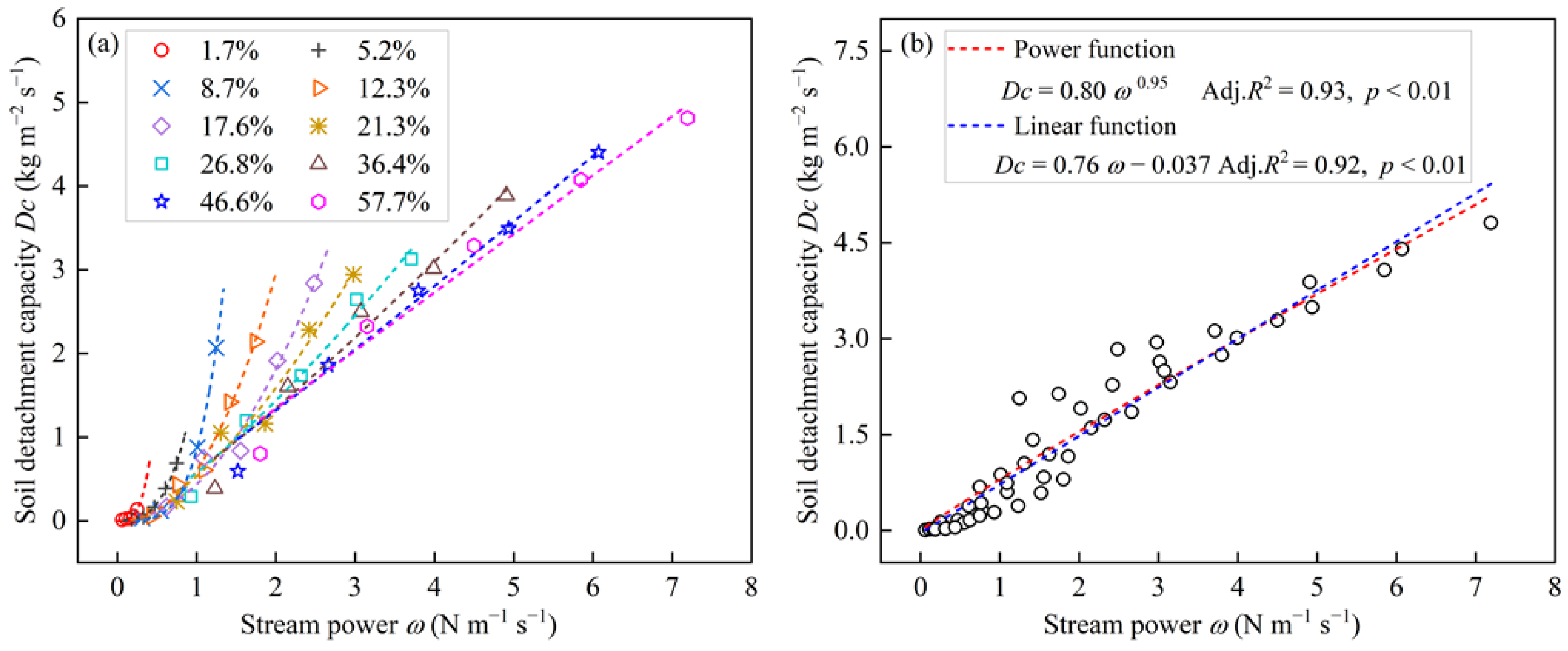
3.3. The Effect of Stream Power on Soil Detachment Capacity

The relationships between Dc and stream power are shown in

Table 4. Relationship between the soil detachment capacity and stream power in different slope gradients.

Slope Gradient %	Power Function Dc = a4 ω b4				Linear Function Dc = k4 (ω–ωc)
	a4	b4	Adj. R2	p	k4	ωc	Adj. R2	p
1.7	15.82	3.44	0.94	<0.010	0.60	0.072	0.71	0.047
5.2	1.66	3.01	0.99	<0.010	1.20	0.25	0.87	0.014
8.7	0.85	4.05	0.99	<0.010	2.07	0.45	0.76	0.033
12.3	0.60	2.29	0.98	<0.010	1.58	0.50	0.92	<0.010
17.6	0.43	2.06	0.97	<0.010	1.40	0.62	0.91	<0.010
21.3	0.53	1.57	0.96	<0.010	1.19	0.58	0.95	<0.010
26.8	0.57	1.32	0.97	<0.010	1.03	0.57	0.99	<0.010
36.4	0.59	1.20	0.96	<0.010	0.91	0.58	0.97	<0.010
46.6	0.62	1.09	0.98	<0.010	0.81	0.58	0.99	<0.010
57.7	0.66	1.02	0.96	<0.010	0.73	0.28	0.97	<0.010
1.7–57.7	0.80	0.95	0.93	<0.010	0.76	0.049	0.92	<0.010

Note: Dc is the soil detachment capacity (kg·m⁻²·s⁻¹); ω is the stream power (N·m⁻¹·s⁻¹); a₄ and b₄ are the coefficient and index of power function, respectively; k₄ is the coefficient of linear function; ω_c is the critical stream power (N·m⁻¹·s⁻¹).

. The Adj. R² of the power function was 1.05% to 32.39% higher than that of a linear function in 1.7–21.3% slopes, and it was only 1.01% to 2.02% lower than that of a linear function in 26.8–57.7% slopes. Overall, Dc increased as a power function with stream power increasing in different slope gradients (Figure 5). The performance of stream power under all combinations of slope gradients was 1.06% to 6.06% lower than that under different slope gradients. However, the slope effect of Dc is not ignored for different slope gradients. Based on the power function equations in different slope gradients in Table 4, the stream power calculated by the maximum Dc of 4.81 kg·s⁻¹·m⁻² in this study increased from 0.71 to 7.01 N·m⁻¹·s⁻¹ (887.32%) with an increasing slope gradient and is calculated by the minimum Dc of 0.011 kg·s⁻¹·m⁻² that changed from 0.018 to 0.34 N·m⁻¹·s⁻¹ (1788.89%) in different slope gradients. Moreover, the Dc calculated by the maximum stream power of 7.19 N·m⁻¹·s⁻¹ decreased from 14020.31 to 4.94 kg·s⁻¹·m⁻² (99.96%) with an increasing slope gradient and is calculated by the minimum stream power of 0.063 N·m⁻¹·s⁻¹ that changed from 0.000011 to 0.039 kg·s⁻¹·m⁻² in different slope gradients, which showed a difference of three orders of magnitude. These results indicated that the equations established by the given slope gradient have great uncertainty when the boundary range was extended.

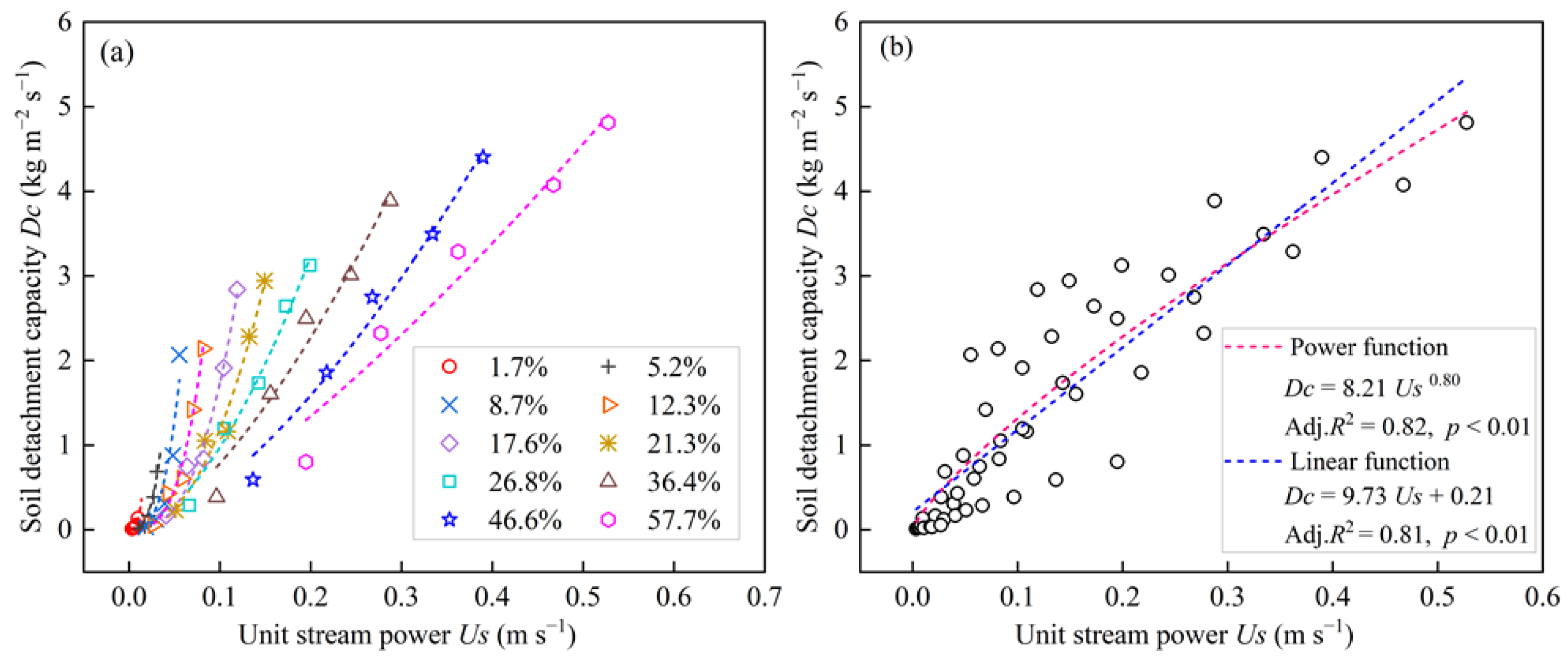
3.4. The Effect of Unit Stream Power on Soil Detachment Capacity

Table 5. Relationship between soil detachment capacity and unit stream power in different slope gradients.

Slope Gradient %	Power Function Dc = a5 Us b5				Linear Function Dc = k5 (Us–Usc)
	a5	b5	Adj. R2	p	k5	Usc	Adj. R2	p
1.7	238,466.60	3.13	0.94	<0.010	17.53	0.0038	0.67	0.057
5.2	34,907.71	3.13	0.97	<0.010	32.58	0.014	0.80	0.027
8.7	13,919.94	3.10	0.91	<0.010	35.13	0.019	0.69	0.040
12.3	5126.22	3.10	0.97	<0.010	36.94	0.031	0.86	0.014
17.6	946.12	2.74	0.97	<0.010	39.58	0.049	0.88	<0.010
21.3	207.81	2.24	0.96	<0.010	29.98	0.055	0.91	<0.010
26.8	52.18	1.73	0.98	<0.010	24.27	0.063	0.97	<0.010
36.4	26.83	1.53	0.96	<0.010	18.89	0.075	0.98	<0.010
46.6	19.34	1.55	0.98	<0.010	14.86	0.093	0.99	<0.010
57.7	11.51	1.34	0.94	<0.010	11.38	0.097	0.96	<0.010
1.7–57.7	8.21	0.80	0.82	<0.010	9.73	-0.022	0.81	<0.010

Note: Dc is the soil detachment capacity (kg·m⁻²·s⁻¹); Us is the unit stream power (m·s⁻¹); a₅ and b₅ are the coefficient and index of power function, respectively; k₅ is the coefficient of linear function; Us_c is the critical unit stream power (m·s⁻¹).

and Figure 6 show the relationships between Dc and unit stream power in different slope gradients. In 1.7–26.8% slopes, the Adj. R² of the power function was 1.03% to 40.30% higher than that of the linear function. In 36.4–57.7% slopes, the Adj. R² of the power function was only 1.01% to 2.08% lower than that of a linear function. For all combinations of slope gradients, the Adj. R² of the power function (0.82) was slightly higher than that of the linear function (0.81). However, there was a slope effect between Dc and unit stream power in Figure 6. Based on the power function equations in different slope gradients in Table 5, the unit stream power calculated by the maximum Dc of 4.81 kg·s⁻¹·m⁻² in this study increased from 0.032 to 0.52 m·s⁻¹ (1525.00%) with an increasing slope gradient and is calculated by the minimum Dc of 0.011 kg·s⁻¹·m⁻² that changed from 0.0045 to 0.016 m·s⁻¹ (255.56%) in different slope gradients. Moreover, the Dc calculated by the maximum unit stream power of 0.53 m·s⁻¹ decreased from 32,227.29 to 4.88 kg·s⁻¹·m⁻² (99.98%) with an increasing slope gradient and is calculated by the minimum unit stream power of 0.0034 m·s⁻¹ that changed from 0.00011 to 0.0056 kg·s⁻¹·m⁻² (4990.91%) in different slope gradients.

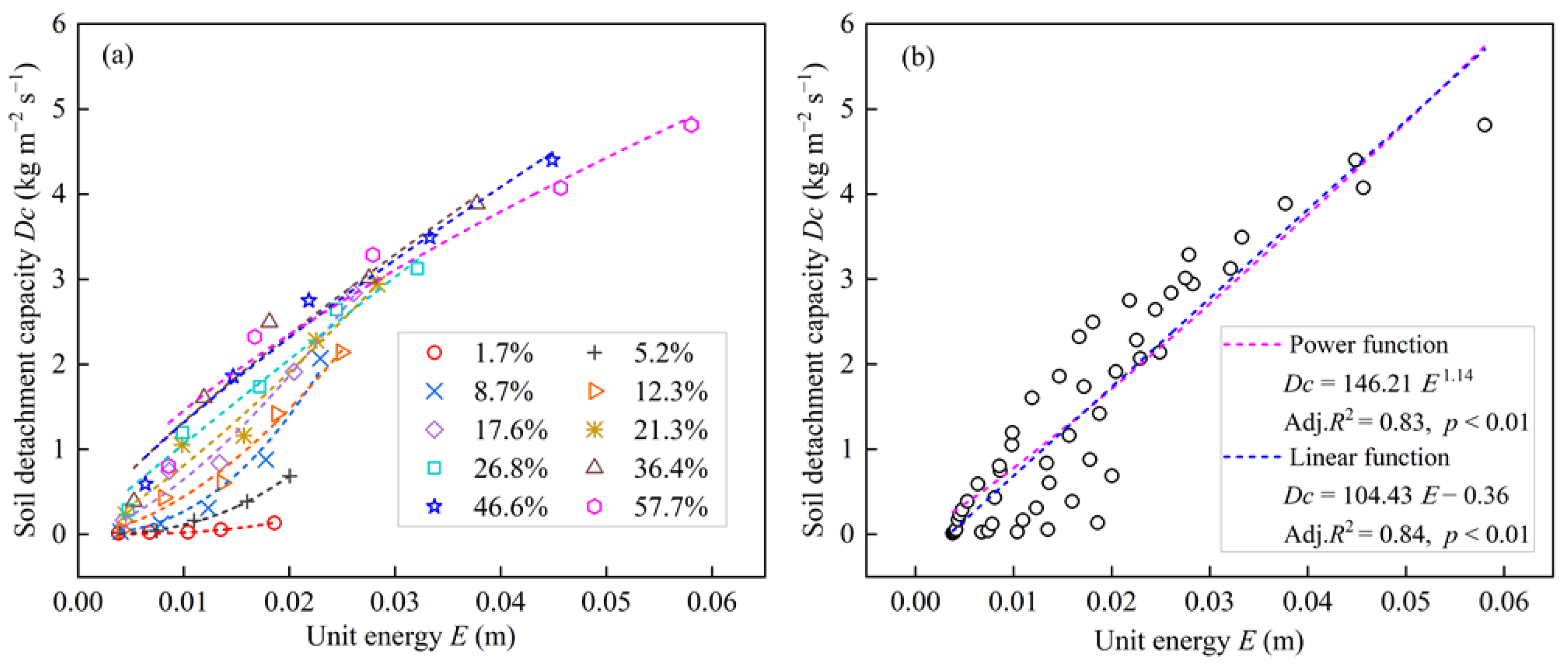
3.5. The Effect of Unit Energy on Soil Detachment Capacity

Table 6. Relationship between soil detachment capacity and unit energy in different slope gradients.

Slope Gradient %	Power Function Dc = a6 E b6				Linear Function Dc = k6 (E–Ec)
	a6	b6	Adj. R2	p	k6	Ec	Adj. R2	p
1.7	19,708.05	2.98	0.96	<0.010	8.00	0.0044	0.80	0.026
5.2	18,130.64	2.60	0.99	<0.010	41.77	0.0055	0.91	<0.010
8.7	14,855.03	2.37	0.98	<0.010	91.20	0.0050	0.90	< 0.010
12.3	1289.04	1.73	0.98	<0.010	99.36	0.0045	0.94	< 0.010
17.6	743.64	1.53	0.98	<0.010	119.21	0.0037	0.95	< 0.010
21.3	241.68	1.24	0.96	<0.010	110.64	0.0023	0.95	< 0.010
26.8	85.70	0.95	0.97	<0.010	103.76	0.00046	0.99	< 0.010
36.4	60.06	0.83	0.95	<0.010	101.92	-0.0023	0.93	< 0.010
46.6	56.90	0.82	0.97	<0.010	95.09	-0.0034	0.96	< 0.010
57.7	35.13	0.69	0.94	<0.010	73.83	-0.010	0.90	< 0.010
1.7–57.7	146.21	1.14	0.83	<0.010	104.43	0.0034	0.84	< 0.010

Note: Dc is the soil detachment capacity (kg·m⁻²·s⁻¹); E is the unit energy (m); a₆ and b₆ are the coefficient and index of power function, respectively; k₆ is the coefficient of linear function; E _c is the critical unit E (m).

and Figure 7 show the response equation of Dc to unit energy. The Adj. R² of the power function was 1.04% to 20.00% higher than that of the linear function except for the slope gradient of 26.8%. Overall, the power functions were superior to the linear functions for different slope gradients, although the Adj. R² of the power function was 1.19% lower than that of the linear function for all combinations of slope gradients. When the maximum Dc was 4.81 kg·s⁻¹·m⁻², the unit energy calculated by power function in different slope gradients changed from 0.034 to 0.061 m (79.41%). When the minimum Dc was 0.011 kg·s⁻¹·m⁻², the unit energy calculated by the power function decreased from 0.0080 to 0.0000084 m (99.90%) in different slope gradients. Moreover, the Dc calculated by the maximum unit energy of 0.058 m changed from 4.08 to 17.44 kg·s⁻¹·m⁻² (327.45%) in different slope gradients, which was calculated by the minimum unit energy of 0.0038 m that increased from 0.0012 to 0.75 kg·s⁻¹·m⁻² (62,400.00%) with an increasing slope gradient, which showed a difference of two orders of magnitude.

4. Discussion

4.1. Modeling the Soil Detachment Capacity Using Different Hydrodynamic Parameters

The quantification of Dc is necessary to establish a process-based soil erosion model [1,4,6,16]. Different hydrodynamic parameters were used to estimate Dc. There were different opinions on the hydrodynamic parameters that best describe the Dc. Some studies indicated that the flow shear stress exhibits the best performance for simulating the Dc [15,19]. Li et al. [33] indicated that there was a similar performance for flow shear stress and stream power for estimating Dc. Parhizkar et al. [27] showed that the unit stream power was an optimal hydrodynamic parameter for estimating Dc. However, most studies have found that the stream power was the best predictor for Dc compared with other hydrodynamic parameters of flow shear stress and unit stream power [11,14,17,34,35]. In this study, it was observed that the correlation between stream power and Dc was the highest (Figure 1). For all combinations of slope gradients, the Adj. R² of the power relationship between Dc and stream power was 27.40%, 13.42%, 12.05%, and 9.41% higher than it was between Dc and flow shear stress, unit stream power, unit energy, and flow velocity, respectively. For the linear relationship between Dc and hydrodynamic parameter, the Adj. R² of stream power was 33.33%, 13.58%, 9.52%, and 9.52% higher than it of flow shear stress, unit stream power, unit energy, and flow velocity, respectively. These results further indicated that the best predictor of Dc was the stream power, and the soil detachment capacity was more closely related to flow energy than to force [36].

Some studies indicated that using the linear function of the hydrodynamic parameter to characterize Dc could better represent the physical process of soil detachment [37,38]. For example, the slope of the linear relationship between Dc and flow shear stress was defined as soil erodibility, and the intercept was defined as critical flow shear stress in WEPP [4]. Soil erodibility and critical flow shear stress were usually considered to remain constant for a given soil property and vegetation condition [39]. However, we found that they were changed with the slope gradient in Table 3. The soil erodibility increased from 0.80 to 2.97 s·m⁻¹ and decreased to 1.86 s·m⁻¹, and the critical flow shear stress increased from 0.33 to 4.26 Pa with an increasing slope gradient in this study. If the linear functions of other hydrodynamic parameters have the same definitions as WEPP, the variations in soil erodibility and critical hydrodynamic parameters also had obvious differences with increasing slope gradients (Table 2, Table 4, Table 5 and Table 6). These results indicated that soil erodibility and critical hydrodynamic parameters were very sensitive to slope gradients. The use of fixed values to extend to different slopes had great limitations. A similar result was also found by Nearing et al. [9], namely that applying a linear flow shear stress model to the entire range of data collected had limitations. Moreover, it also showed that the linear relationship did not necessarily have a clear physical meaning.

4.2. Slope Effect of the Relationship Between Soil Detachment Capacity and Hydrodynamic Parameters

Previous studies have shown that shallow overland flow and soil detachment on gentle slopes are different from those on steep slopes [9,10]. However, the differences in the dynamic mechanisms of soil detachment between steep and gentle slopes remain unclear. In this study, we found that the relationships between Dc and hydrodynamic parameters were affected by slope gradient. As shown in Table 1 and Table 3, the relationships between Dc and flow depth and flow shear stress shifted from power functions for slope gradient of ≤17.6% to linear functions for slope gradient of ≥21.3%. Although the form of power function relationship between Dc and other hydrodynamic parameters (flow velocity, stream power, unit stream power, and unit energy) did not change, their coefficients and indexes differed markedly under varying slope gradient conditions (Table 2, Table 4, Table 5 and Table 6). The above phenomenon resulted in a great uncertainty when the boundary range was extended for the equations established by a given slope gradient. Based on the optimal functional relationship, the values of hydrodynamic characteristics (flow velocity, flow shear stress, stream power, unit stream power, and unit energy) calculated by the maximum and minimum Dc in this study changed by 19.91–95,138.10%, and the values of Dc calculated by the maximum and minimum hydrodynamic characteristics could differ by up to nine orders of magnitude.

The effects of different hydrodynamic parameters on Dc under varying slope gradient conditions were showed in Figure 8. The index of power function decreased exponentially (Adj. R² > 0.78, p < 0.01) as the slope gradient increased for different hydrodynamic parameters. However, the coefficient of power function showed different trends with increasing slope gradient. Further analysis found that the coefficient of flow velocity first increased as a power function (Adj. R² = 0.96, p < 0.01) and then decreased as a power function (Adj. R² = 0.88, p < 0.01) with increasing slope gradient (Figure 8a). For flow shear stress and stream power, their coefficients first decreased as a power function (Adj. R² = 0.99, p < 0.01) and then increased as power and exponential functions (Adj. R² > 0.83, p < 0.01) with increasing slope gradient (Figure 8b,c), respectively. The coefficients of unit stream power and unit energy decreased as a power function with increasing slope gradient (Figure 8d,e). These results indicated that the relationships between Dc and hydrodynamic parameters were usually unstable in different slope gradient conditions. This finding was consistent with the result of Parhizkar et al. [16] that the varying slope gradients have different influences on Dc resulting in the change in relationships between Dc and hydrodynamic parameters. The flow velocity and depth are basic parameters in calculating flow shear stress, stream power, unit stream power, and unit energy. As shown in Figure 2 and Figure 3, the effects of flow depth and flow velocity affect Dc depend directly on the slope gradients. For the shallow overland flow, the change in flow velocity and depth are very complex due to the interaction between viscous stress and Reynolds stress [40]. The flow structure becomes extremely unstable as the slope gradient increased, and there are great differences in different sediment concentration conditions [41]. The effect of slope gradient on other hydrodynamic parameters actually depends on the flow velocity and flow depth. Therefore, the slope effect appeared in establishing the soil detachment equations using different hydrodynamic parameters, which was further confirmed by correlation analysis in Figure 1. Multiple regression analysis showed that Dc (kg·m⁻²·s⁻¹) could be well predicted by slope gradient (S, %), flow velocity (v, m·s⁻¹), and flow depth (h, mm), as follows:

$$Dc=0.051v^{1.07}{h}^{1.93}{S}^{0.96}\mathrm{Adj}.R^2=0.96,p<0.01$$

(6)

Compared to the power function of the single hydrodynamic parameter (such as flow shear stress, stream power, unit stream power, and unit energy), the Adj. R² of Equation (6) increased by 2.23–39.13%. This result further indicated that the Dc was affected by the interaction of slope gradient, flow velocity, and flow depth. However, it is very necessary to study the hydrodynamic mechanism of overland flow on slopes based on a high-resolution particle image velocimetry system in future work, which can provide more microscopic information on the changes in the flow fields and help to find the theoretical basis for the slope effect of soil detachment.

5. Conclusions

The runoff scouring experiment was conducted to gain insights into the slope effect of soil detachment capacity at the varying hydrodynamic characteristics. The relationships between Dc and hydrodynamic parameters were affected by slope gradient. There were obvious differences in the extrapolation of the equations of soil detachment capacity established by different slope gradients. Overall, the power function of hydrodynamic parameters was superior to the linear function in different slope gradients. The soil erodibility and critical hydrodynamic characteristic defined by linear function were variable rather than constant due to the effect of slope gradient. The stream power was best predictor for Dc compared with other hydrodynamic parameters. For all combinations of slope gradients, the Adj. R² of the power relationship between Dc and stream power was 27.40%, 13.42%, 12.05%, and 9.41% higher than it was between Dc and flow shear stress, unit stream power, unit energy, and flow velocity, respectively. The coefficient and index of power function for different hydrodynamic parameters showed a trend change with increasing slope gradient, indicating that there was a slope effect on Dc. These results confirmed that the soil detachment equation established by a given slope gradient have great uncertainty when the boundary range was extended. Further analysis found that Dc could be well predicted using a power combination equation of slope gradient, flow velocity, and flow depth (Adj. R² = 0.96). However, it is necessary to adopt more advanced technical means to study the microscopic information of the overland flow field changes, which will help to find the theoretical basis for the slope effect of soil detachment. Moreover, these results need to be further validated in different climatic regions and soil types.

References

1. Guo, D.W.; Yu, B.F.; Fu, X.D.; Li, T.J. Improved hillslope erosion module for the Digital Yellow-River Model. J. Hydrol. Eng. 2015, 20, C4014011. [Google Scholar] [CrossRef]
2. Wang, C.F.; Fu, X.D.; Wang, B.; Gong, Z.; Zhang, G.; Wang, X.P. Modeling feedback processes between soil detachment and sediment transport along hillslopes on the Loess Plateau of China. Sci. Total Environ. 2023, 901, 166032. [Google Scholar] [CrossRef] [PubMed]
3. Foster, G.R.; Meyer, L.D. A closed-form soil erosion equation for upland areas. In Sedimentation Symposium; Einstein, H.A., Shen, H.W., Eds.; Colorado State University: Fort Collins, CO, USA, 1972; pp. 12–19. [Google Scholar]
4. Nearing, M.A.; Foster, G.R.; Lane, L.J.; Finkner, S.C. A process-based soil erosion model for USDA-Water Erosion Prediction Project technology. Trans. ASAE 1989, 32, 1587–1593. [Google Scholar] [CrossRef]
5. Morgan, R.P.C.; Quinton, J.N.; Smith, R.E.; Govers, G.; Poesen, J.W.A.; Auerswald, K.; Chisci, G.; Torri, D.; Styczen, M.E. The European Soil Erosion Model (EUROSEM): A dynamic approach for predicting sediment transport from fields and small catchments. Earth Surf. Proc. Landf. 1998, 23, 527–544. [Google Scholar] [CrossRef]
6. Wang, C.F.; Fu, X.D.; Zhang, X.M.; Wang, X.P.; Zhang, G.; Gong, Z. Modeling soil erosion dynamic processes along hillslopes with vegetation impact across different land uses on the Loess Plateau of China. Catena 2024, 243, 108202. [Google Scholar] [CrossRef]
7. Misra, R.K.; Rose, C.W. Application and sensitivity analysis of process-based erosion model GUEST. Eur. J. Soil Sci. 1996, 47, 593–604. [Google Scholar] [CrossRef]
8. Zhang, G.; An, C.G.; Wang, C.F.; Wang, B.J.; Yu, B.F.; Fu, X.D. Numerical modeling of effects of vegetation restoration on runoff and sediment yield on the Loess Plateau, China. Catena 2024, 247, 108501. [Google Scholar] [CrossRef]
9. Nearing, M.A.; Simanton, J.R.; Norton, L.D.; Bulygin, S.J.; Stone, J. Soil erosion by surface water flow on a stony, semiarid hillslope. Earth Surf. Proc. Landf. 1999, 24, 677–686. [Google Scholar] [CrossRef]
10. Zhang, G.H.; Liu, Y.M.; Han, Y.F.; Zhang, X.C. Sediment transport and soil detachment on steep slopes: I. Transport capacity estimation. Soil Sci. Soc. Am. J. 2009, 73, 1291–1297. [Google Scholar] [CrossRef]
11. Shen, N.; Wang, Z.L.; Guo, Q.; Zhang, Q.W.; Wu, B.; Liu, J.E.; Ma, C.Y.; Delang, C.O.; Zhang, F.B. Soil detachment capacity by rill flow for five typical loess soils on the Loess Plateau of China. Soil Tillage Res. 2021, 213, 105159. [Google Scholar] [CrossRef]
12. Yao, C.; Zhang, Q.W.; Wang, C.F.; Ren, J.; Li, H.K.; Wang, H.; Wu, F.Q. Response of sediment transport capacity to soil properties and hydraulic parameters in the typical agricultural regions of the Loess Plateau. Sci. Total Environ. 2023, 879, 163090. [Google Scholar] [CrossRef] [PubMed]
13. Nearing, M.A.; Bradford, J.M.; Parker, S.C. Soil detachment by shallow flow at low slopes. Soil Sci. Soc. Am. J. 1991, 55, 339–344. [Google Scholar] [CrossRef]
14. Zhang, J.; Chen, X.Y.; Tao, T.T.; Han, W.; Wang, X.; Luo, F.L.; Tan, W.T.; Kong, L.Y.; Feng, T.; Zhu, P.Z. Field simulation experiment on the relationships between hydrodynamics and soil detachment rate in formed rills. Catena 2023, 233, 107540. [Google Scholar] [CrossRef]
15. Cao, L.X.; Zhang, K.L.; Dai, H.L.; Guo, Z.L. Modeling soil detachment on unpaved road surfaces on the Loess Plateau. Trans. ASABE 2011, 54, 1377–1384. [Google Scholar] [CrossRef]
16. Parhizkar, M.; Shabanpour, M.; Khaledian, M.; Asadi, H. The evaluation of soil detachment capacity induced by vegetal species based on the comparison between natural and planted forests. J. Hydrol. 2021, 595, 126041. [Google Scholar] [CrossRef]
17. Mirzaee, S.; Ghorbani-Dashtaki, S. Deriving and evaluating hydraulics and detachment models of rill erosion for some calcareous soils. Catena 2018, 164, 107–115. [Google Scholar] [CrossRef]
18. Zhang, G. Study on hydraulic properties of shallow flow. Adv. Water Sci. 2002, 13, 159–165. (In Chinese) [Google Scholar]
19. Gimenez, R.; Govers, G. Flow detachment by concentrated flow on smooth and irregular beds. Soil Sci. Soc. Am. J. 2002, 66, 1475–1483. [Google Scholar] [CrossRef]
20. Wang, D.D.; Wang, Z.L.; Shen, N.; Chen, H. Modeling soil detachment capacity by rill flow using hydraulic parameters. J. Hydrol. 2016, 535, 473–479. [Google Scholar] [CrossRef]
21. Parhizkar, M.; Shabanpour, M.; Miralles, I.; Cerdà, A.; Tanaka, N.; Asadi, H.; Lucas-Borja, M.E.; Zema, D.A. Evaluating the effects of forest tree species on rill detachment capacity in a semi-arid environment. Ecol. Eng. 2021, 161, 106158. [Google Scholar] [CrossRef]
22. Rose, C.W.; Williams, J.R.; Sander, G.C.; Barry, D.A. A Mathematical Model of Soil Erosion and Deposition Processes: I. Theory for a Plane Land Element. Soil Sci. Soc. Am. J. 1983, 47, 991–995. [Google Scholar] [CrossRef]
23. Ciampalini, R.; Torri, D. Detachment of soil particles by shallow flow: Sampling methodology and observations. Catena 1998, 32, 37–53. [Google Scholar] [CrossRef]
24. Liu, B.Y.; Nearing, M.; Shi, P.J.; Jia, Z.W. Slope length effects on soil loss for steep slopes. Soil Sci. Soc. Am. J. 2000, 64, 1759–1763. [Google Scholar] [CrossRef]
25. Zhao, G.J.; Yue, X.L.; Tian, P.; Mu, X.M.; Xu, W.L.; Wang, F.; Gao, P.; Sun, W.Y. Comparison of the suspended sediment dynamics in two Loess Plateau catchments, China. Land Degrad. Dev. 2017, 28, 1398–1411. [Google Scholar] [CrossRef]
26. Shi, Z.H.; Liu, Q.J.; Zhang, H.Y.; Wang, L.; Xuan, H.; Fang, N.F.; Yue, Z.J. Study on soil erosion and conservation in the past 10 Years: Progress and prospects. Acta Pedol. Sin. 2020, 57, 1117–1127. (In Chinese) [Google Scholar]
27. Parhizkar, M.; Shabanpour, M.; Lucas-Borja, M.E.; Zema, D.A. Variability of rill detachment capacity with sediment size, water depth and soil slope in forest soils: A flume experiment. J. Hydrol. 2021, 601, 126625. [Google Scholar] [CrossRef]
28. Bagnold, R.A. An Approach to the Sediment Transport Problem from General Physics. Geological Survey Professional Paper; 422–J; US Government Printing Office: Washington, DC, USA, 1966. [Google Scholar]
29. Yang, C.T. Unit stream power and sediment transport. J. Hydraul. Div. 1972, 98, 1805–1826. [Google Scholar] [CrossRef]
30. Foster, G.R.; Huggins, L.F.; Meyer, L.D. A Laboratory Study of Rill Hydraulics: II. Shear Stress Relationships. Trans. ASAE 1984, 27, 797–804. [Google Scholar] [CrossRef]
31. Shen, E.S.; Liu, G.; Dan, C.X.; Chen, X.Y.; Ye, S.M.; Li, R.Q.; Li, H.X.; Zhang, Q.; Zhang, Y.; Guo, Z. Estimating Manning’s coefficient n for sheet flow during rainstorms. Catena 2023, 226, 107093. [Google Scholar] [CrossRef]
32. Cai, Z.K.; Xie, J.B.; Chen, Y.C.; Yang, Y.S.; Wang, C.F.; Wang, J. Rigid Vegetation Affects Slope Flow Velocity. Water 2024, 16, 2240. [Google Scholar] [CrossRef]
33. Li, T.Y.; Li, S.Y.; Liang, C.; He, B.H.; Bush, R.T. Erosion vulnerability of sandy clay loam soil in Southwest China: Modeling soil detachment capacity by flume simulation. Catena 2019, 178, 90–99. [Google Scholar] [CrossRef]
34. Xiao, H.; Liu, G.; Liu, P.L.; Zheng, F.L.; Zhang, J.Q.; Hu, F.N. Response of soil detachment rate to the hydraulic parameters of concentrated flow on steep loessial slopes on the Loess Plateau of China. Hydrol. Process. 2017, 31, 2613–2621. [Google Scholar] [CrossRef]
35. Zhu, X.L.; Fu, S.H.; Wu, Q.Y.; Wang, A.J. Soil detachment capacity of shallow overland flow in Earth-Rocky Mountain Area of Southwest China. Geoderma 2020, 361, 114021. [Google Scholar] [CrossRef]
36. Zhang, G.H.; Liu, B.Y.; Nearing, M.A.; Huang, C.H.; Zhang, K.L. Soil detachment by shallow flow. Trans. ASAE 2002, 45, 351–357. [Google Scholar]
37. Laflen, J.M.; Elliot, W.J.; Simanton, J.R.; Holzhey, C.S.; Kohl, K.D. WEPP: Soil erodibility experiments for rangeland and cropland soils. J. Soil Water Conserv. 1991, 46, 39–44. [Google Scholar]
38. Su, Z.L.; Zhang, G.H.; Yi, T.; Liu, F. Soil detachment capacity by overland flow for soils of the Beijing region. Soil Sci. 2014, 179, 446–453. [Google Scholar] [CrossRef]
39. Flanagan, D.C.; Frankenberger, J.R.; Ascough, J.C., II. WEPP: Model use, calibration, and validation. Trans. ASABE 2012, 55, 1463–1477. [Google Scholar] [CrossRef]
40. Yang, P.P.; Zhang, H.L.; Wang, Y.Q.; Wang, Y.J.; Wang, Y.T. Overland flow velocities measured using a high-resolution particle image velocimetry system. J. Hydrol. 2020, 590, 125225. [Google Scholar] [CrossRef]
41. Niu, M.F.; Sun, S.X.; Gong, Z.W. Experimental analysis on characteristics of vertical velocity of overland flow on low sediment concentration. J. Lanzhou Jiaotong Univ. 2022, 41, 96–102. (In Chinese) [Google Scholar]
Figure 1. Pearson correlation coefficient between hydrodynamic parameters and soil detachment capacity.
Water 17 00028 g001
Figure 2. The effect of flow depth on the soil detachment capacity in different slope gradients.
Water 17 00028 g002
Figure 3. The effect of flow velocity on soil detachment capacity (a) in different slope gradients and (b) in all combinations of slope gradients.
Water 17 00028 g003
Figure 4. The effect of flow shear stress on soil detachment capacity (a) in different slope gradients and (b) in all combinations of slope gradients.
Water 17 00028 g004
Figure 5. The effect of stream power on soil detachment capacity (a) in different slope gradients and (b) in all combinations of slope gradients.
Water 17 00028 g005
Figure 6. The effect of unit stream power on soil detachment capacity (a) in different slope gradients and (b) in all combinations of slope gradients.
Water 17 00028 g006
Figure 7. The effect of unit energy on soil detachment capacity (a) in different slope gradients and (b) in all combinations of slope gradients.
Water 17 00028 g007
Figure 8. Slope effect of soil detachment capacity for different hydraulic parameters.
Water 17 00028 g008