

A Versatile Workflow for Building 3D Hydrogeological Models Combining Subsurface and Groundwater Flow Modelling: A Case Study from Southern Sardinia (Italy)

 ,
,
Abstract
1. Introduction
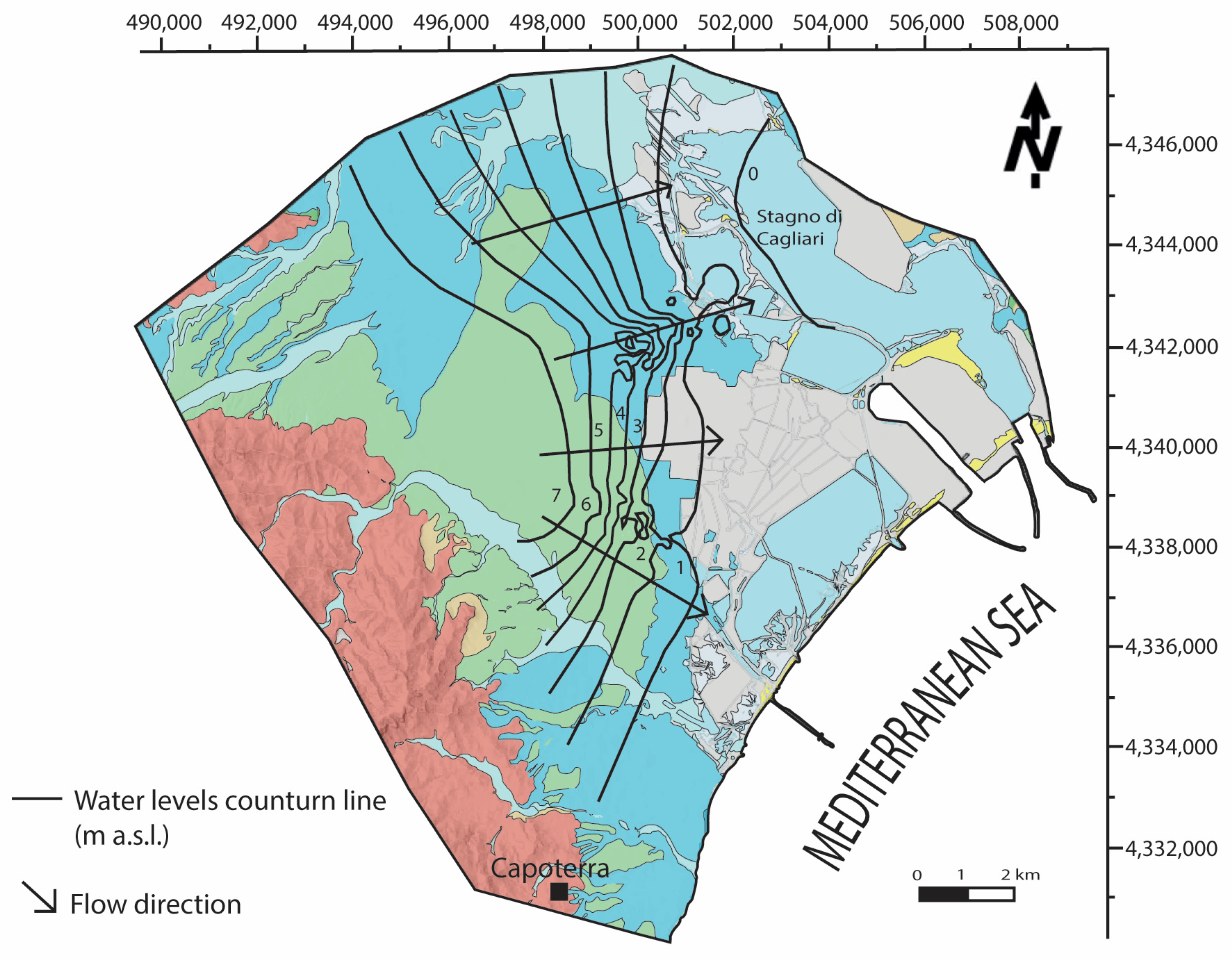
2. Geological and Hydrogeological Setting
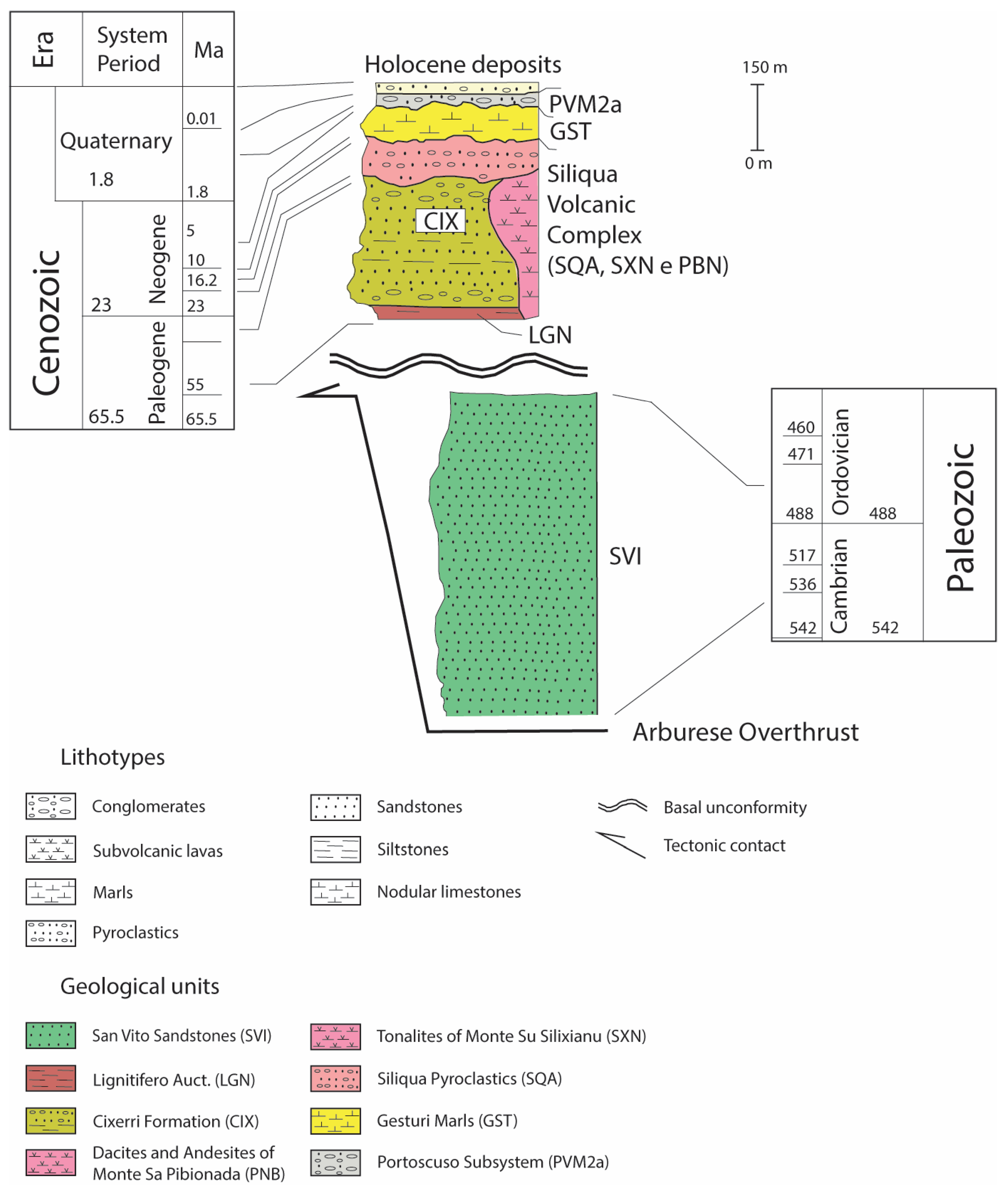
2.1. Geological Setting
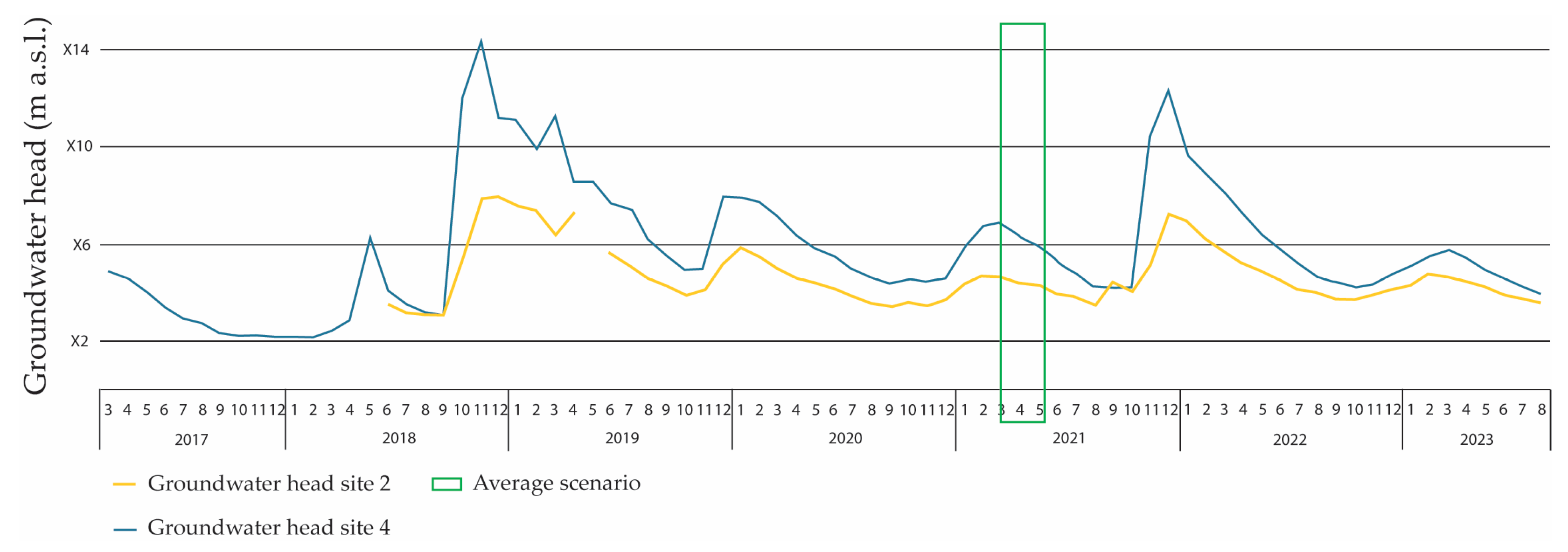
2.2. Hydrogeological Setting
3. Data and Methods
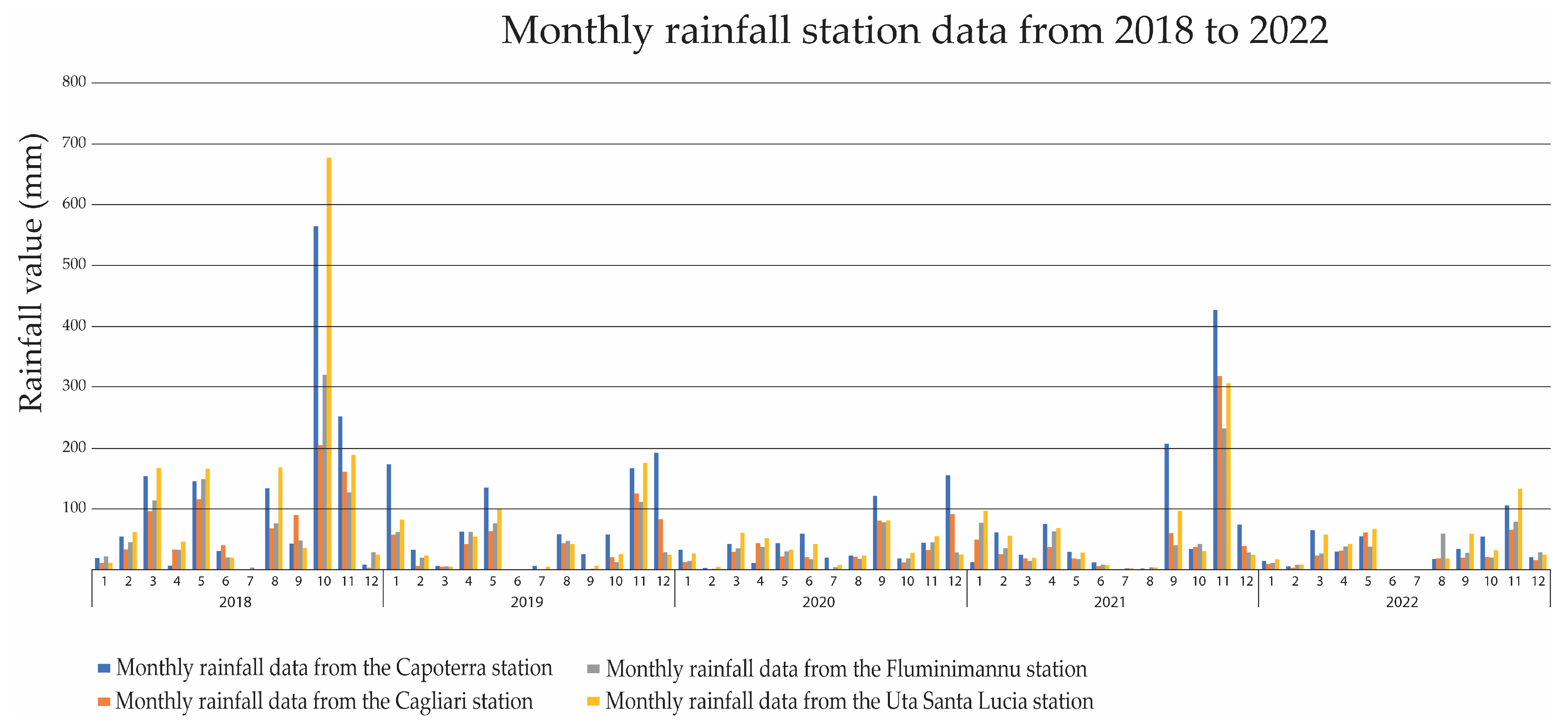
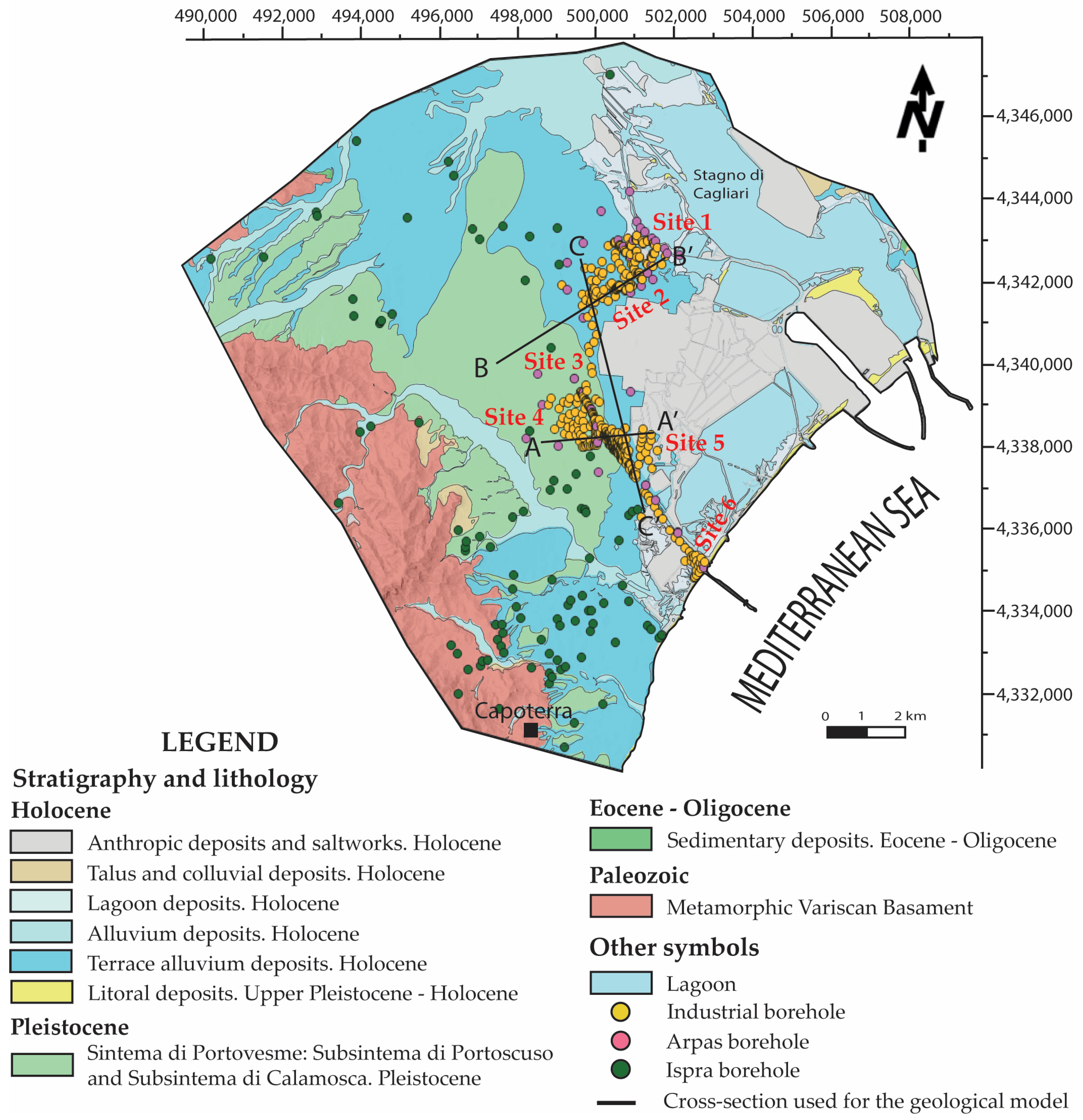
3.1. Data Source
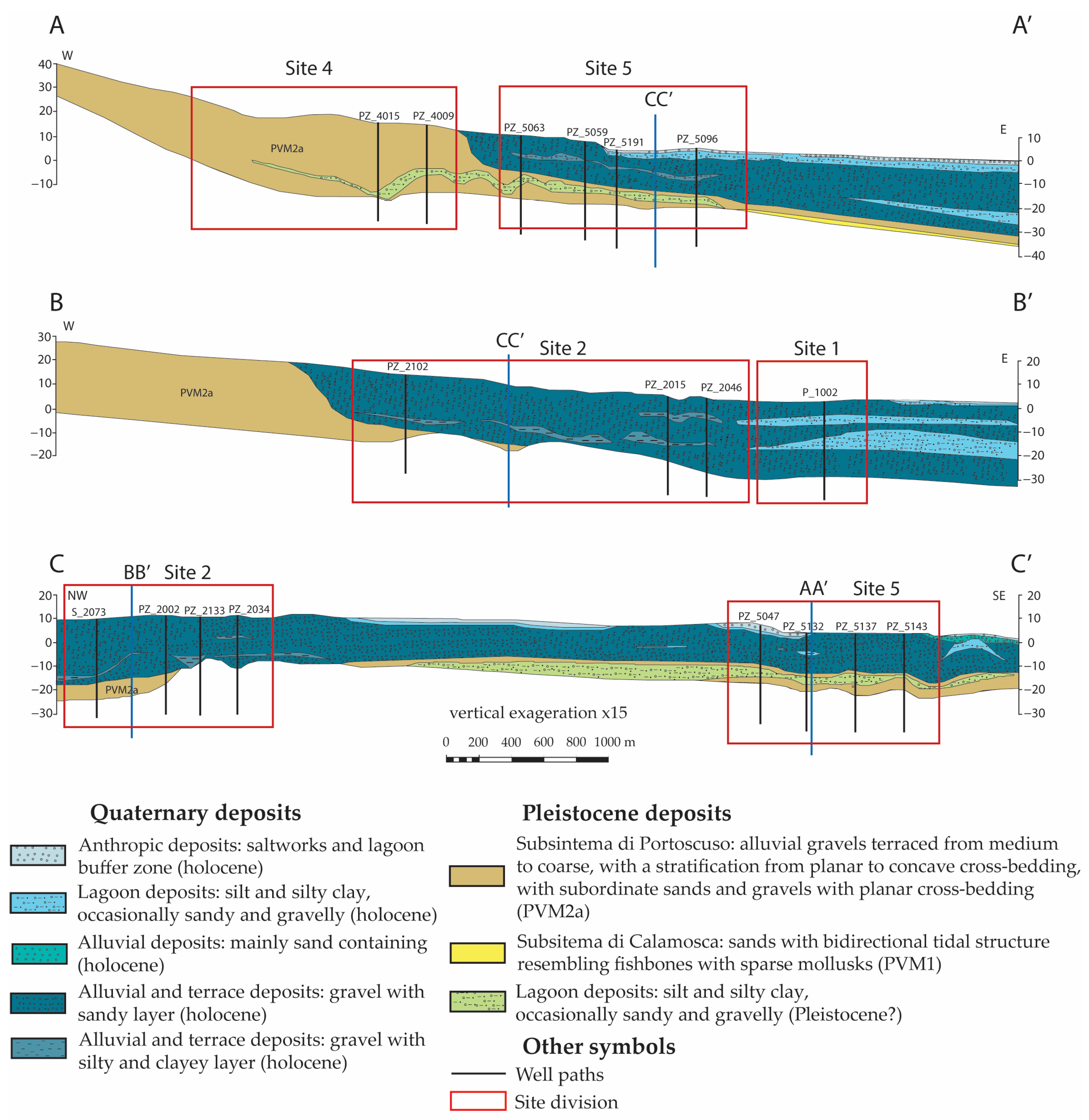
3.2. Sedimentological Model
3.3. Conceptual Model
3.4. Three-Dimensional Hydrogeological Model
3.5. Numerical Groundwater Flow Model
- h is the hydraulic head (piezometric level).
- Ss is the specific storage of the porous media.
- K represents the hydraulic conductivity tensor.
- W includes all external water sources or sinks (e.g., recharge, pumping) [90].
4. Results
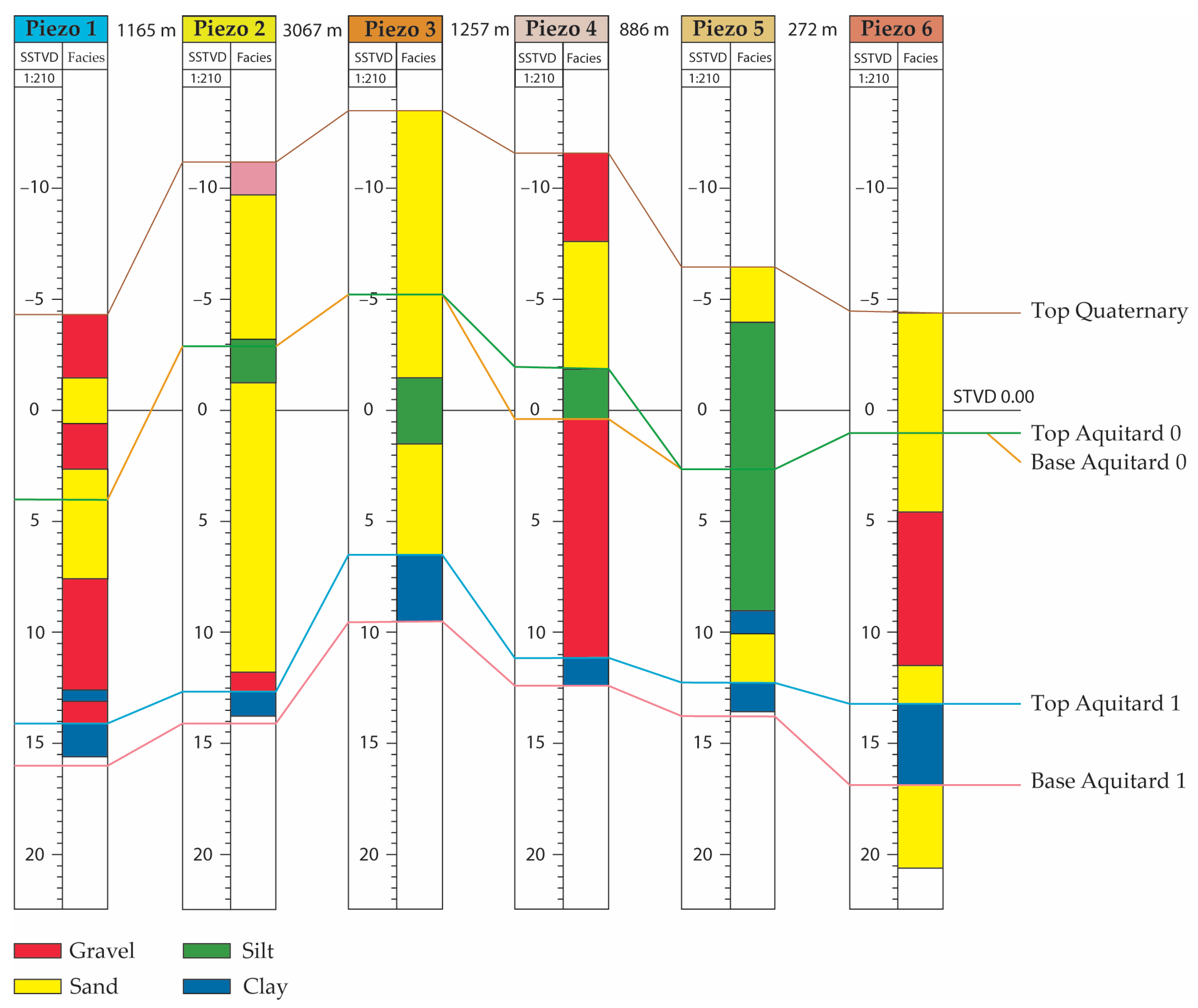
4.1. Hydrostratigraphic Model
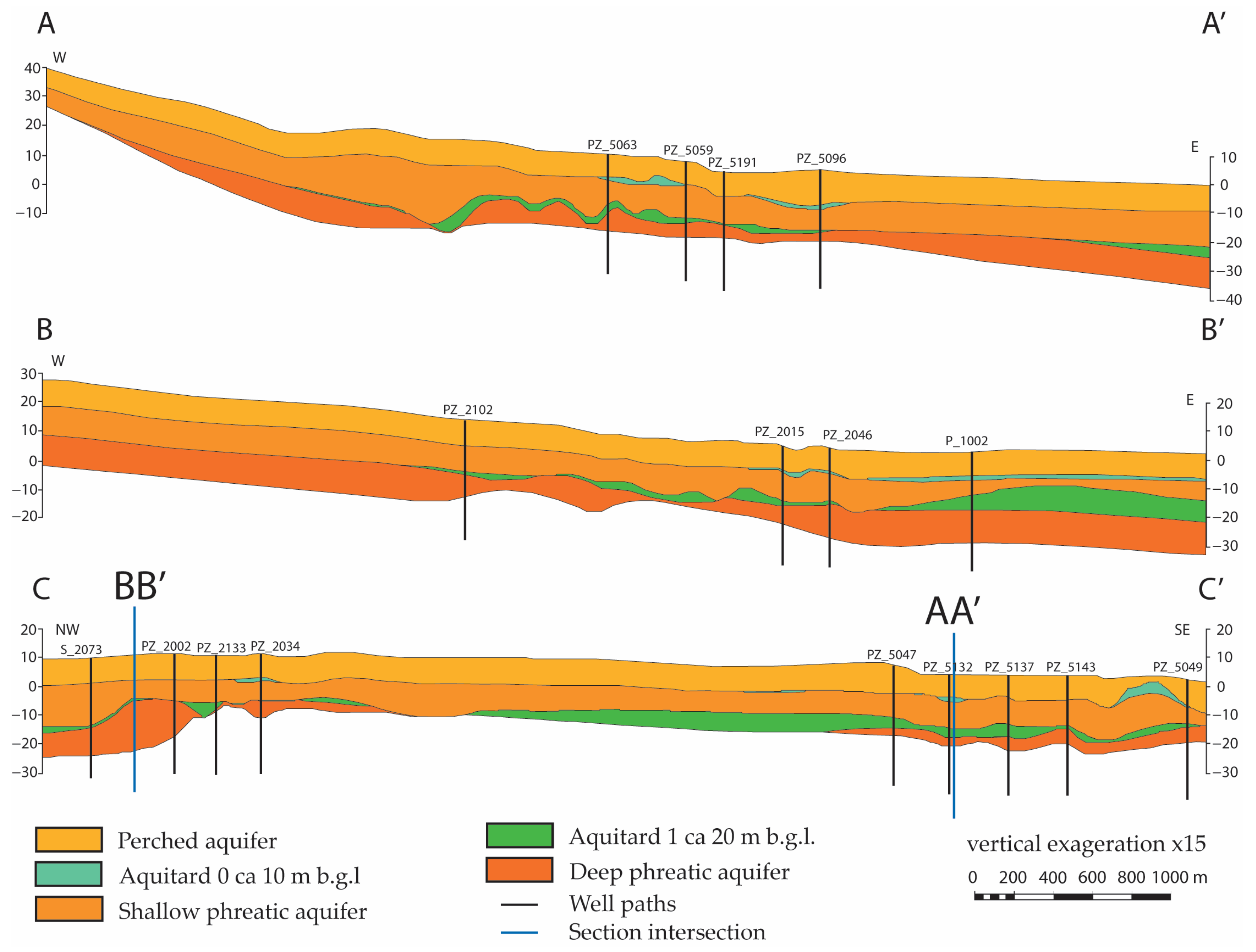
4.2. Hydrogeological Model
4.3. Numerical Groundwater Flow Model and Calibration
5. Discussion
6. Conclusions
Author Contributions
Funding
Data Availability Statement
Acknowledgments
Conflicts of Interest
Appendix A

| OBS | H Simulated | H Misurated | Absolute Error | Squared Error |
|---|---|---|---|---|
| Pz_4_01 | 2.78 | 2.497 | −0.283 | 8.01 × 10⁻² |
| Pz_4_02 | 2.25 | 3.139 | 0.889 | 7.90 × 10⁻¹ |
| Pz_4_03 | 3.03 | 3.183 | 0.153 | 2.35 × 10⁻² |
| Pz_4_04 | 6.52 | 2.947 | −3.573 | 1.28 × 101 |
| Pz_4_05 | 6.39 | 2.658 | −3.732 | 1.39 × 101 |
| Pz_4_06 | 3.55 | 3.314 | −0.236 | 5.57 × 10⁻² |
| Pz_4_07 | 2.68 | 2.712 | 0.032 | 1.01 × 10⁻³ |
| Pz_4_08 | 3.22 | 3.261 | 0.041 | 1.70 × 10⁻³ |
| Pz_4_09 | 2.78 | 2.777 | −0.003 | 9.41 × 10⁻⁶ |
| Pz_4_10 | 3.10 | 2.671 | −0.429 | 1.84 × 10⁻¹ |
| Pz_4_11 | 3.92 | 3.638 | −0.282 | 7.94 × 10⁻² |
| Pz_4_12 | 4.85 | 3.885 | −0.965 | 9.31 × 10⁻¹ |
| Pz_4_13 | 3.72 | 3.556 | −0.164 | 2.70 × 10⁻² |
| Pz_4_14 | 2.65 | 3.379 | 0.729 | 5.31 × 10⁻¹ |
| Pz_4_15 | 2.04 | 2.993 | 0.953 | 9.09 × 10⁻¹ |
| Pz_4_16 | 2.95 | 2.980 | 0.030 | 9.08 × 10⁻⁴ |
| Pz_4_17 | 5.28 | 4.134 | −1.146 | 1.31 × 100 |
| Pz_4_18 | 4.45 | 3.874 | −0.576 | 3.32 × 10⁻¹ |
| Pz_4_19 | 4.11 | 3.720 | −0.390 | 1.52 × 10⁻¹ |
| Pz_4_20 | 5.05 | 4.177 | −0.873 | 7.63 × 10⁻¹ |
| Pz_4_21 | 4.23 | 3.892 | −0.338 | 1.14 × 10⁻¹ |
| Pz_4_22 | 5.58 | 4.529 | −1.051 | 1.10 × 100 |
| Pz_4_23 | 5.28 | 4.453 | −0.827 | 6.84 × 10⁻¹ |
| Pz_4_24 | 4.75 | 4.221 | −0.529 | 2.80 × 10⁻¹ |
| Pz_4_25 | 6.70 | 5.606 | −1.094 | 1.20 × 100 |
| Pz_4_26 | 6.40 | 5.771 | −0.629 | 3.96 × 10⁻¹ |
| Pz_4_27 | 4.08 | 2.875 | −1.205 | 1.45 × 100 |
| Pz_4_28 | 3.94 | 3.099 | −0.841 | 7.07 × 10⁻¹ |
| Pz_4_29 | 6.13 | 4.624 | −1.506 | 2.27 × 100 |
| Pz_4_30 | 3.72 | 3.589 | −0.131 | 1.73 × 10⁻² |
| Pz_4_31 | 2.90 | 3.265 | 0.365 | 1.33 × 10⁻¹ |
| Pz_4_32 | 3.51 | 3.836 | 0.326 | 1.06 × 10⁻¹ |
| Pz_4_33 | 4.15 | 3.780 | −0.370 | 1.37 × 10⁻¹ |
| Pz_4_34 | 3.43 | 3.834 | 0.404 | 1.63 × 10⁻¹ |
| Pz_4_35 | 6.56 | 5.094 | −1.466 | 2.15 × 100 |
| Pz_4_36 | 5.40 | 4.812 | −0.588 | 3.45 × 10⁻¹ |
| Pz_4_37 | 4.09 | 4.436 | 0.346 | 1.20 × 10⁻¹ |
| Pz_4_38 | 5.98 | 5.105 | −0.875 | 7.66 × 10⁻¹ |
| Pz_4_39 | 5.11 | 4.867 | −0.243 | 5.89 × 10⁻² |
| Pz_4_40 | 4.25 | 4.473 | 0.223 | 4.96 × 10⁻² |
| Pz_4_41 | 4.27 | 4.358 | 0.088 | 7.70 × 10⁻³ |
| Pz_4_42 | 3.45 | 3.422 | −0.028 | 7.65 × 10⁻⁴ |
| Pz_4_43 | 2.80 | 2.887 | 0.087 | 7.53 × 10⁻³ |
| Pz_4_44 | 2.90 | 2.924 | 0.024 | 5.65 × 10⁻⁴ |
| Pz_4_45 | 3.99 | 4.359 | 0.369 | 1.36 × 10⁻¹ |
| Pz_4_46 | 3.61 | 4.167 | 0.557 | 3.10 × 10⁻¹ |
| Pz_4_47 | 3.43 | 3.965 | 0.535 | 2.86 × 10⁻¹ |
| Pz_4_48 | 3.55 | 3.768 | 0.218 | 4.74 × 10⁻² |
| Pz_4_49 | 3.28 | 3.536 | 0.256 | 6.54 × 10⁻² |
| Pz_4_50 | 3.01 | 3.383 | 0.373 | 1.39 × 10⁻¹ |
| Pz_4_51 | 2.84 | 3.237 | 0.397 | 1.58 × 10⁻¹ |
| Pz_4_52 | 2.83 | 2.972 | 0.142 | 2.00 × 10⁻² |
| Pz_4_53 | 2.98 | 2.939 | −0.041 | 1.70 × 10⁻³ |
| Pz_4_54 | 2.96 | 2.835 | −0.125 | 1.56 × 10⁻² |
| Pz_4_55 | 2.76 | 2.758 | −0.002 | 4.93 × 10⁻⁶ |
| Pz_4_56 | 2.75 | 2.712 | −0.038 | 1.46 × 10⁻³ |
| Pz_4_57 | 2.69 | 2.671 | −0.019 | 3.53 × 10⁻⁴ |
| Pz_4_58 | 2.63 | 2.639 | 0.009 | 7.92 × 10⁻⁵ |
| Pz_4_59 | 2.52 | 2.609 | 0.089 | 8.00 × 10⁻³ |
| Pz_4_60 | 6.28 | 2.706 | −3.574 | 1.28 × 101 |
| Pz_4_61 | 2.64 | 2.823 | 0.183 | 3.35 × 10⁻² |
| Pz_4_62 | 2.81 | 3.002 | 0.192 | 3.69 × 10⁻² |
| Pz_2_01 | 4.87 | 7.166 | 2.296 | 5.27 × 100 |
| Pz_2_02 | 6.82 | 6.755 | −0.065 | 4.22 × 10⁻³ |
| Pz_2_03 | 4.97 | 7.406 | 2.436 | 5.94 × 100 |
| Pz_2_04 | 5.46 | 5.805 | 0.345 | 1.19 × 10⁻¹ |
| Pz_2_05 | 5.16 | 5.205 | 0.045 | 2.01 × 10⁻³ |
| Pz_2_06 | 3.29 | 4.402 | 1.112 | 1.24 × 100 |
| Pz_2_07 | 4.22 | 4.287 | 0.067 | 4.55 × 10⁻³ |
| Pz_2_08 | 3.45 | 3.467 | 0.017 | 2.98 × 10⁻⁴ |
| Pz_2_09 | 1.49 | 2.654 | 1.164 | 1.35 × 100 |
| Pz_2_10 | 1.09 | −0.717 | −1.807 | 3.27 × 100 |
| Pz_2_11 | 4.02 | 8.061 | 4.041 | 1.63 × 101 |
| Pz_2_12 | 4.17 | 4.952 | 0.782 | 6.11 × 10⁻¹ |
| Pz_2_13 | 1.64 | 0.800 | −0.840 | 7.06 × 10⁻¹ |
| Pz_2_14 | 1.06 | −0.016 | −1.076 | 1.16 × 100 |
| Pz_2_15 | 1.12 | 0.057 | −1.063 | 1.13 × 100 |
| Pz_2_16 | 1.10 | 0.088 | −1.012 | 1.02 × 100 |
| Pz_2_17 | 0.92 | −0.099 | −1.019 | 1.04 × 100 |
| Pz_2_18 | 0.97 | −0.008 | −0.978 | 9.57 × 10⁻¹ |
| Pz_2_19 | 1.02 | −0.165 | −1.185 | 1.40 × 100 |
| Pz_2_20 | 1.70 | −0.267 | −1.967 | 3.87 × 100 |
| Pz_2_21 | 0.47 | 1.532 | 1.062 | 1.13 × 100 |
| Pz_2_22 | 1.25 | 1.763 | 0.513 | 2.63 × 10⁻¹ |
| Pz_2_23 | 2.01 | 2.346 | 0.336 | 1.13 × 10⁻¹ |
| Pz_2_24 | 1.54 | 2.179 | 0.639 | 4.08 × 10⁻¹ |
| Pz_2_25 | 1.88 | 1.837 | −0.043 | 1.88 × 10⁻³ |
| Pz_2_26 | 1.44 | 1.135 | −0.305 | 9.29 × 10⁻² |
| Pz_2_27 | 4.69 | 7.466 | 2.776 | 7.70 × 100 |
| Pz_2_28 | 4.06 | 5.814 | 1.754 | 3.08 × 100 |
| Pz_2_29 | 4.15 | 5.912 | 1.762 | 3.10 × 100 |
| Pz_2_30 | 3.59 | 4.954 | 1.364 | 1.86 × 100 |
| Pz_2_31 | 2.41 | 1.186 | −1.224 | 1.50 × 100 |
| Pz_2_32 | 4.07 | 5.147 | 1.077 | 1.16 × 100 |
| Pz_2_33 | 6.84 | 7.492 | 0.652 | 4.25 × 10⁻¹ |
| Pz_2_34 | 3.52 | 2.921 | −0.599 | 3.59 × 10⁻¹ |
| Pz_2_35 | 1.34 | 0.722 | −0.618 | 3.82 × 10⁻¹ |
| Pz_2_36 | 3.26 | 5.763 | 2.503 | 6.26 × 100 |
| Pz_2_37 | 5.42 | 8.064 | 2.644 | 6.99 × 100 |
| Pz_2_38 | 2.44 | 3.756 | 1.316 | 1.73 × 100 |
| Pz_2_39 | 4.79 | 4.078 | −0.712 | 5.07 × 10⁻¹ |
| Pz_2_40 | 6.57 | 6.347 | −0.223 | 4.98 × 10⁻² |
| Pz_2_41 | 6.96 | 6.199 | −0.761 | 5.79 × 10⁻¹ |
| Pz_2_42 | 1.82 | 3.204 | 1.384 | 1.92 × 100 |
| Pz_2_43 | 6.63 | 4.875 | −1.755 | 3.08 × 100 |
| Pz_2_44 | 2.71 | 2.471 | −0.239 | 5.69 × 10⁻² |
| Pz_2_45 | 2.10 | 1.968 | −0.132 | 1.73 × 10⁻² |
| Pz_2_46 | 1.12 | −0.598 | −1.718 | 2.95 × 100 |
| Pz_2_47 | 2.27 | −0.716 | −2.986 | 8.92 × 100 |
| Pz_2_48 | 1.48 | 0.373 | −1.107 | 1.22 × 100 |
| Pz_2_49 | 1.31 | 0.268 | −1.042 | 1.09 × 100 |
| Pz_2_50 | 1.45 | 2.139 | 0.689 | 4.75 × 10⁻¹ |
| Pz_2_51 | 1.65 | 2.967 | 1.317 | 1.73 × 100 |
| Pz_2_52 | 3.64 | 2.692 | −0.948 | 9.00 × 10⁻¹ |
| Pz_2_53 | 1.42 | 1.000 | −0.420 | 1.77 × 10⁻¹ |
| Pz_2_54 | 1.53 | 1.626 | 0.096 | 9.23 × 10⁻³ |
| Pz_2_55 | 1.12 | −0.681 | −1.801 | 3.24 × 100 |
| Pz_2_56 | 2.10 | 0.883 | −1.217 | 1.48 × 100 |
| Pz_2_57 | 1.49 | 2.311 | 0.821 | 6.75 × 10⁻¹ |
| Pz_2_58 | 4.57 | 4.278 | −0.292 | 8.52 × 10⁻² |
| Pz_2_59 | 5.62 | 5.260 | −0.360 | 1.30 × 10⁻¹ |
| Pz_2_60 | 1.39 | 3.812 | 2.422 | 5.87 × 100 |
| Pz_2_61 | 1.47 | 1.277 | −0.193 | 3.71 × 10⁻² |
| Pz_2_62 | 3.13 | 2.169 | −0.961 | 9.23 × 10⁻¹ |
| Pz_2_63 | 3.39 | 3.257 | −0.133 | 1.77 × 10⁻² |
| Pz_2_64 | 3.17 | 5.882 | 2.712 | 7.35 × 100 |
| Pz_2_65 | 4.58 | 6.307 | 1.727 | 2.98 × 100 |
| Pz_2_66 | 4.39 | 6.675 | 2.285 | 5.22 × 100 |
| Pz_2_67 | 6.11 | 6.881 | 0.771 | 5.94 × 10⁻¹ |
| Pz_2_68 | 5.86 | 10.186 | 4.326 | 1.87 × 100 |
| Pz_2_69 | 1.45 | 1.757 | 0.307 | 9.42 × 10⁻² |
| Pz_2_70 | 4.80 | 5.011 | 0.211 | 4.44 × 10⁻² |
| Pz_2_71 | 4.16 | 6.094 | 1.934 | 3.74 × 100 |
| Pz_2_72 | 2.08 | 2.109 | 0.029 | 8.35 × 10⁻⁴ |
| Pz_2_73 | 4.01 | 5.947 | 1.937 | 3.75 × 100 |
| Pz_2_74 | 4.25 | 5.740 | 1.490 | 2.22 × 100 |
| Pz_2_75 | 6.54 | 5.929 | −0.611 | 3.73 × 10⁻¹ |
| Pz_5_01 | 1.45 | 1.731 | 0.281 | 7.89 × 10⁻² |
| Pz_5_02 | 2.14 | 2.346 | 0.206 | 4.26 × 10⁻² |
| Pz_5_03 | 1.91 | 1.869 | −0.041 | 1.71 × 10⁻³ |
| Pz_5_04 | 2.62 | 2.232 | −0.388 | 1.51 × 10⁻¹ |
| Pz_5_05 | 2.40 | 1.767 | −0.632 | 3.99 × 10⁻¹ |
| Pz_5_06 | 1.87 | 1.637 | −0.233 | 5.41 × 10⁻² |
| Pz_5_07 | 2.56 | 1.744 | −0.841 | 7.08 × 10⁻¹ |
| Pz_5_08 | 1.42 | 1.364 | −0.057 | 3.23 × 10⁻³ |
| Pz_5_09 | 1.11 | 1.091 | −0.019 | 3.79 × 10⁻⁴ |
| Pz_5_10 | 1.53 | 1.875 | 0.345 | 1.19 × 10⁻¹ |
| Pz_5_11 | 1.11 | 1.616 | 0.506 | 2.56 × 10⁻¹ |
| Pz_5_12 | 1.68 | 1.659 | −0.017 | 2.82 × 10⁻⁴ |
| Pz_5_13 | 0.95 | 1.735 | 0.783 | 6.13 × 10⁻¹ |
| Pz_5_14 | 1.65 | 1.585 | −0.060 | 3.61 × 10⁻³ |
| Pz_6_01 | 0.24 | 0.176 | −0.067 | 4.51 × 10⁻³ |
| Pz_6_02 | 0.27 | 0.325 | 0.052 | 2.66 × 10⁻³ |
| Pz_6_03 | 0.31 | 0.324 | 0.019 | 3.58 × 10⁻⁴ |
| Pz_6_04 | 0.28 | 0.361 | 0.079 | 6.26 × 10⁻³ |
| Pz_6_05 | 0.33 | 0.417 | 0.091 | 8.35 × 10⁻³ |
| Pz_6_06 | 0.16 | 0.220 | 0.059 | 3.48 × 10⁻³ |
| Pz_6_07 | 0.11 | 0.334 | 0.218 | 4.74 × 10⁻² |
| Pz_6_08 | 0.19 | 0.401 | 0.213 | 4.53 × 10⁻² |
| Pz_6_09 | 0.45 | 0.170 | −0.281 | 7.87 × 10⁻² |
| Pz_6_10 | 0.15 | 0.295 | 0.146 | 2.13 × 10⁻² |
| Pz_6_11 | 0.27 | 0.405 | 0.140 | 1.95 × 10⁻² |
| Pz_6_12 | 0.23 | 0.213 | −0.017 | 2.84 × 10⁻⁴ |
| Pz_6_13 | 0.30 | 0.264 | −0.031 | 9.47 × 10⁻⁴ |
| Pz_6_14 | 0.30 | 0.377 | 0.074 | 5.50 × 10⁻³ |
| Pz_6_15 | 0.11 | 0.325 | 0.215 | 4.63 × 10⁻² |
References
- Cidu, R.; Biddau, R.; Fanfani, L. Impact of past mining activity on the quality of groundwater in SW Sardinia (Italy). J. Geochem. Explor. 2009, 100, 125–132. [Google Scholar] [CrossRef]
- Lee, J.Y.; Moon, S.H.; Yun, S.T. Contamination of groundwater by arsenic and other constituents in an industrial complex. Environ. Earth Sci. 2010, 60, 65–79. [Google Scholar] [CrossRef]
- Biddau, R.; Cidu, R. Groundwater contamination: Environmental issues and case studies in Sardinia (Italy). In Threats to the Quality of Groundwater Resources: Prevention and Control; Springer: Berlin/Heidelberg, Germany, 2016; pp. 53–76. [Google Scholar]
- Tiwari, A.K.; Orioli, S.; De Maio, M. Assessment of groundwater geochemistry and diffusion of hexavalent chromium contamination in an industrial town of Italy. J. Contam. Hydrol. 2019, 225, 103503. [Google Scholar] [CrossRef] [PubMed]
- Li, P.; Karunanidhi, D.; Subramani, T.; Srinivasamoorthy, K. Sources and Consequences of Groundwater Contamination. Arch. Environ. Contam. Toxicol. 2021, 80, 1–10. [Google Scholar] [CrossRef]
- Kinzelbach, W. Groundwater Modelling: An Introduction with Sample Programs in BASIC; Developments in Water Science; Elsevier: Amsterdam, The Netherlands; Oxford, UK; New York, NY, USA; Tokyo, Japan, 1986; ISBN 978-0-444-42582-9. [Google Scholar]
- Chiang, W.-H. 3D-Groundwater Modeling with PMWIN; Springer: Berlin/Heidelberg, Germany, 2005; p. 411. [Google Scholar]
- Barazzuoli, P.; Nocchi, M.; Rigati, R.; Salleolini, M. A conceptual and numerical model for groundwater management: A case study on a coastal aquifer in southern Tuscany, Italy. Hydrogeol. J. 2008, 8, 1557–1576. [Google Scholar] [CrossRef]
- Singh, A. Groundwater resources management through the applications of simulation modeling: A review. Sci. Total Environ. 2014, 499, 414–423. [Google Scholar] [CrossRef]
- Ghiglieri, G.; Carletti, A.; Da Pelo, S.; Cocco, F.; Funedda, A.; Loi, A.; Manta, F.; Pittalis, D. Three-dimensional hydrogeological reconstruction based on geological depositional model: A case study from the coastal plain of Arborea (Sardinia, Italy). Eng. Geol. 2016, 207, 103–114. [Google Scholar] [CrossRef]
- Smaoui, H.; Zouhri, L.; Ouahsine, A.; Carlier, E. Modelling of groundwater flow in heterogeneous porous media by finite element method. Hydrol. Process. 2012, 26, 558–569. [Google Scholar] [CrossRef]
- Lal, A.; Datta, B. Performance evaluation of homogeneous and heterogeneous ensemble models for groundwater salinity predictions: A regional-scale comparison study. Water Air Soil Pollut. 2020, 231, 320. [Google Scholar] [CrossRef]
- Hudon-Gagnon, E.; Chesnaux, R.; Cousineau, P.A.; Rouleau, A. A hydrostratigraphic simplification approach to build 3D groundwater flow numerical models: Example of a Quaternary deltaic deposit aquifer. Environ. Earth Sci. 2015, 74, 4671–4683. [Google Scholar] [CrossRef]
- Mukherjee, A.; Fryar, A.E.; Howell, P.D. Regional hydrostratigraphy and groundwater flow modeling in the arsenic-affected areas of the western Bengal basin, West Bengal, India. Hydrogeol. J. 2007, 15, 1397–1418. [Google Scholar] [CrossRef]
- El-Azhari, A.; Karaoui, I.; Brahim, Y.A.; Azhar, M.; Chehbouni, A.; Bouchaou, L. Analyses of groundwater level in a data-scarce region based on assessed precipitation products and machine learning. Groundw. Sustain. Dev. 2024, 26, 101299. [Google Scholar] [CrossRef]
- Chicco, J.M.; Mandrone, G. Modelling the Energy Production of a Borehole Thermal Energy Storage (BTES) System. Energies 2022, 15, 9587. [Google Scholar] [CrossRef]
- Chicco, J.M.; Fonte, L.; Mandrone, G.; Tartaglino, A.; Vacha, D. Hybrid (Gas and Geothermal) greenhouse simulations aimed at optimizing investment and operative costs: A case study in NW Italy. Energies 2023, 16, 3931. [Google Scholar] [CrossRef]
- Wu, Y.; Wang, W.; Toll, M.; Alkhoury, W.; Sauter, M.; Kolditz, O. Development of a 3D groundwater model based on scarce data: The Wadi Kafrein catchment/Jordan. Environ. Earth Sci. 2011, 64, 771–785. [Google Scholar] [CrossRef]
- Brassington, F.C.; Younger, P.L. A proposed framework for hydrogeological conceptual modelling. Water Environ. J. 2010, 24, 261–273. [Google Scholar] [CrossRef]
- Enemark, T.; Peeters, L.J.; Mallants, D.; Batelaan, O. Hydrogeological conceptual model building and testing: A review. J. Hydrol. 2019, 569, 310–329. [Google Scholar] [CrossRef]
- Neuman, S.P.; Wierenga, P.J. A Comprehensive Strategy of Hydrogeologic Modeling and Uncertainty Analysis for Nuclear Facilities and Sites; Report NUREG/CR-6805; The University of Arizona: Tucson, AZ, USA, 2003. [Google Scholar]
- Klingbeil, R.; Kleineidam, S.; Asprion, U.; Aigner, T.; Teutsch, G. Relating lithofacies to hydrofacies: Outcrop-based hydrogeological characterisation of Quaternary gravel deposits. Sediment. Geol. 1999, 129, 299–310. [Google Scholar] [CrossRef]
- Weissmann, G.S.; Carle, S.F.; Fogg, G.E. Three-dimensional hydrofacies modeling based on soil surveys and transition probability geostatistics. Water Resour. Res. 1999, 35, 1761–1770. [Google Scholar] [CrossRef]
- Heinz, J.; Aigner, T. Hierarchical dynamic stratigraphy in various Quaternary gravel deposits, Rhine glacier area (SW Germany): Implications for hydrostratigraphy. Int. J. Earth Sci. 2003, 92, 923–938. [Google Scholar] [CrossRef]
- Pugin, A.J.M.; Oldenborger, G.A.; Cummings, D.I.; Russell, H.A.; Sharpe, D.R. Architecture of buried valleys in glaciated Canadian Prairie regions based on high resolution geophysical data. Quat. Sci. Rev. 2014, 86, 13–23. [Google Scholar] [CrossRef]
- Di Salvo, C.; Di Luzio, E.; Mancini, M.; Moscatelli, M.; Capelli, G.; Cavinato, G.P.; Mazza, R. GIS-based hydrostratigraphic modeling of the city of Rome (Italy): Analysis of the geometric relationships between a buried aquifer in the Tiber Valley and the confining hydrostratigraphic complexes. Hydrogeol. J. 2012, 20, 1549. [Google Scholar] [CrossRef]
- Irace, A.; Clemente, P.; Piana, F.; De Luca, D.A.; Polino, R.; Violanti, D.; Mosca, P.; Trenkwalder, S.; Natalicchio, M.; Ossella, L.; et al. Hydrostratigraphy of the late Messinian-Quaternary basins in the southern Piedmont (northwestern Italy). Mem. Descr. Carta Geol. It. 2010, 90, 133–152. [Google Scholar]
- Anderson, M.P.; Woessner, W.W.; Hunt, R.J. Applied Groundwater Modeling: Simulation of Flow and Advective Transport, 2nd ed.; Elservier: London, UK, 2015; ISBN 9780120581030. [Google Scholar]
- Beven, K. Towards an alternative blueprint for a physically based digitally simulated hydrologic response modelling system. Hydrol. Process. 2002, 16, 189–206. [Google Scholar] [CrossRef]
- Refsgaard, J.C.; Van der Sluijs, J.P.; Brown, J.; Van der Keur, P. A framework for dealing with uncertainty due to model structure error. Adv. Water Resour. 2006, 29, 1586–1597. [Google Scholar] [CrossRef]
- Madsen, R.B.; Høyer, A.S.; Andersen, L.T.; Møller, I.; Hansen, T.M. Geology-driven modeling: A new probabilistic approach for incorporating uncertain geological interpretations in 3D geological modeling. Eng. Geol. 2022, 309, 106833. [Google Scholar] [CrossRef]
- Barfod, A.A.; Møller, I.; Christiansen, A.V.; Høyer, A.S.; Hoffimann, J.; Straubhaar, J.; Caers, J. Hydrostratigraphic modeling using multiple-point statistics and airborne transient electromagnetic methods. Hydrol. Earth Syst. Sci. 2018, 22, 3351–3373. [Google Scholar] [CrossRef]
- Gong, W.; Zhao, C.; Juang, C.H.; Zhang, Y.; Tang, H.; Lu, Y. Coupled characterization of stratigraphic and geo-properties uncertainties—A conditional random field approach. Eng. Geol. 2021, 294, 106348. [Google Scholar] [CrossRef]
- Madsen, R.B.; Kim, H.; Kallesøe, A.J.; Sandersen, P.B.; Vilhelmsen, T.N.; Hansen, T.M.; Christiansen, A.V.; Møller, I.; Hansen, B. 3D multiple-point geostatistical simulation of joint subsurface redox and geological architectures. Hydrol. Earth Syst. Sci. 2021, 25, 2759–2787. [Google Scholar] [CrossRef]
- Stafleu, J.; Maljers, D.; Gunnink, J.L.; Menkovic, A.; Busschers, F.S. 3D modelling of the shallow subsurface of Zeeland, the Netherlands. Neth. J. Geosci. 2011, 90, 293–310. [Google Scholar] [CrossRef]
- Vilhelmsen, T.N.; Auken, E.; Christiansen, A.V.; Barfod, A.S.; Marker, P.A.; Bauer-Gottwein, P. Combining clustering methods with MPS to estimate structural uncertainty for hydrological models. Front. Earth Sci. 2019, 7, 181. [Google Scholar] [CrossRef]
- Zhao, C.; Gong, W.; Li, T.; Juang, C.H.; Tang, H.; Wang, H. Probabilistic characterization of subsurface stratigraphic configuration with modified random field approach. Eng. Geol. 2021, 288, 106138. [Google Scholar] [CrossRef]
- Mackay, D.M.; Roberts, P.V.; Cherry, J.A. Transport of organic contaminants in groundwater. Environ. Sci. Technol. 1985, 19, 384–392. [Google Scholar] [CrossRef] [PubMed]
- Macdonald, R.W.; Harner, T.; Fyfe, J. Recent climate change in the Arctic and its impact on contaminant pathways and interpretation of temporal trend data. Sci. Total Environ. 2005, 342, 5–86. [Google Scholar] [CrossRef]
- Al-Baldawi, B.A. Building a 3D geological model using petrel software for Asmari reservoir, south eastern Iraq. Iraqi J. Sci. 2015, 56, 1750–1762. [Google Scholar]
- Schlumberger. Petrel Seismic-to-Evaluation Software, version 2010; Schlumberger: Houston, TX, USA, 2010.
- Alloisio, S.; Clayton Phair, C.; Cathy Safadi, C. Integrated use of Petrel© and Modflow in the modeling of water injection and effects on a Quaternary aquifer. In Proceedings of the GeoHydro 2011, Quebec City, QC, Canada, 28–31 August 2011. 6p. [Google Scholar]
- Pala, A.; Pecorini, G.; Porcu, A.; Serra, S. Schema geologico strutturale della Sardegna [Geological and structural scheme of Sardinia]. In Ricerche Geotermiche in Sardegna con Particolare Riferimento al Graben del Campidano; CNR-PFE-SPEG-RF-10; CNR: Rome, Italy, 1982. [Google Scholar]
- Arthaud, F.; Matte, P. Late Paleozoic strike-slip faulting in southern Europe and northern Africa: Result of a right-lateral shear zone between the Appalachians and the Urals. Geol. Soc. Am. Bull. 1977, 88, 1305–1320. [Google Scholar] [CrossRef]
- Carmignani, L.; Oggiano, G.; Barca, S.; Conti, P.; Salvadori, I.; Eltrudis, A.; Funedda, A.; Pasci, S. Geologia della Sardegna. Note illustrative della Carta Geologica della Sardegna a scala 1:200,000. In Memorie Descrittive Carta Geologica d’Italia; Istituto Poligrafico e Zecca dello Stato: Rome, Italy, 2001; p. 60. Available online: https://www.academia.edu/16956720/Geologia_della_Sardegna_Note_illustrative_Della_Carta_Geologica_in_Scala_1_200_000 (accessed on 25 May 2024).
- Carmignani, L.; Funedda, A.; Oggiano, G.; Pasci, S. Tectono-sedimentary evolution of southwest Sardinia in the Paleogene: Pyrenaic or Apenninic Dynamic? Geodin. Acta 2004, 17, 275–287. [Google Scholar] [CrossRef]
- Carmignani, L.; Oggiano, G.; Funedda, A.; Conti, P.; Pasci, S. The geological map of Sardinia (Italy) at 1:250,000 scale. J. Maps 2016, 12, 826–835. [Google Scholar] [CrossRef]
- von Raumer, J.F.; Stampfli, G.M.; Bussy, F. Gondwana-derived microcontinents—The constituents of the Variscan and Alpine collisional orogens. Tectonophysics 2003, 365, 7–22. [Google Scholar] [CrossRef]
- von Raumer, J.F.; Stampfli, G.M. The birth of the Rheic Ocean—Early Palaeozoic subsidence patterns and subsequent tectonic plate scenarios. Tectonophysics 2008, 461, 9–20. [Google Scholar] [CrossRef]
- Cassinis, G.; Durand, M.; Ronchi, A. Permian-Triassic continental sequences of Northwest Sardinia and South Provence: Stratigraphic correlations and palaeogeographical implications. Boll. Della Soc. Geol. Ital. 2003, 2, e129. [Google Scholar]
- Di Vincenzo, G.; Carosi, R.; Palmeri, R. The relationship between tectono-metamorphic evolution and argon isotope records in white mica: Constraints from in situ 40Ar–39Ar laser analysis of the Variscan basement of Sardinia. J. Petrol. 2004, 45, 1013–1043. [Google Scholar] [CrossRef]
- Gaggero, L.; Gretter, N.; Langone, A.; Ronchi, A. U–Pb geochronology and geochemistry of late Palaeozoic volcanism in Sardinia (southern Variscides). Geosci. Front. 2017, 8, 1263–1284. [Google Scholar] [CrossRef]
- Ronchi, A.; Sarria, E.; Broutin, J. The “Autuniano Sardo”: Basic features for a correlation through the Western Mediterranean and Paleoeurope. Boll. Della Soc. Geol. Ital. 2008, 127, 655–681. [Google Scholar]
- Casini, L.; Funedda, A.; Oggiano, G. A balanced foreland–hinterland deformation model for the Southern Variscan belt of Sardinia, Italy. Geol. J. 2010, 45, 634–649. [Google Scholar] [CrossRef]
- Casini, L.; Cuccuru, S.; Maino, M.; Oggiano, G.; Tiepolo, M. Emplacement of the Arzachena Pluton (Corsica–Sardinia Batholith) and the geodynamics of incoming Pangaea. Tectonophysics 2012, 544, 31–49. [Google Scholar] [CrossRef]
- Casini, L.; Puccini, A.; Cuccuru, S.; Maino, M.; Oggiano, G. GEOTHERM: A finite difference code for testing metamorphic P–T–t paths and tectonic models. Comput. Geosci. 2013, 59, 171–180. [Google Scholar] [CrossRef]
- Casini, L.; Cuccuru, S.; Puccini, A.; Oggiano, G.; Rossi, P. Evolution of the Corsica–Sardinia Batholith and late-orogenic shearing of the Variscides. Tectonophysics 2015, 646, 65–78. [Google Scholar] [CrossRef]
- Carosi, R.; Montomoli, C.; Tiepolo, M.; Frassi, C. Geochronological constraints on post-collisional shear zones in the Variscides of Sardinia (Italy). Terra Nova 2012, 24, 42–51. [Google Scholar] [CrossRef]
- Cocco, F.; Oggiano, G.; Funedda, A.; Loi, A.; Casini, L. Stratigraphic, magmatic and structural features of Ordovician tectonics in Sardinia (Italy): A review. J. Iber. Geol. 2018, 44, 619–639. [Google Scholar] [CrossRef]
- Stori, L.; Ronchi, A.; López-Gómez, J.; Márquez-Aliaga, A.; Ros-Franch, S.; Goy, A.; Márquez, L.; Gandin, A.; Martín-Chivelet, J. Middle Triassic (Muschelkalk) transgression in the West Tethys: Biostratigraphic evidence from Sardinia (Italy). Palaeoworld 2023, 33, 997–1024. [Google Scholar] [CrossRef]
- Alvarez, W. Rotation of the Corsica–Sardinia microplate. Nat. Phys. Sci. 1972, 235, 103–105. [Google Scholar] [CrossRef]
- Cherchi, A.; Montadert, L. Oligo-Miocene rift of Sardinia and the early history of the western Mediterranean basin. Nature 1982, 298, 736–739. [Google Scholar] [CrossRef]
- Carmignani, L.; Carosi, R.; Di Pisa, A.; Gattiglio, M.; Musumeci, G.; Oggiano, G.; Carlo Pertusati, P. The hercynian chain in Sardinia (Italy). Geodin. Acta 1994, 7, 31–47. [Google Scholar] [CrossRef]
- Carmignani, L.; Decandia, F.A.; Disperati, L.; Fantozzi, P.L.; Lazzarotto, A.; Liotta, D.; Oggiano, G. Relationships between the Tertiary structural evolution of the Sardinia-Corsica-Provençal Domain and the Northern Apennines. Terra Nova 1995, 7, 128–137. [Google Scholar] [CrossRef]
- Funedda, A.; Oggiano, G.; Pasci, S. The Logudoro Basin; a key area for the Tertiary tectono-sedimentary evolution of north Sardinia. Boll. Della Soc. Geol. Ital. 2000, 119, 31–38. [Google Scholar]
- Speranza, F.; Villa, I.M.; Sagnotti, L.; Florindo, F.M.; Cosentino, D.; Cipollari, P.; Mattei, M. Age of the Corsica–Sardinia rotation and Liguro–Provençal Basin spreading: New paleomagnetic and Ar/Ar evidence. Tectonophysics 2002, 347, 231–251. [Google Scholar] [CrossRef]
- Oggiano, G.; Funedda, A.; Carmignani, L.; Pasci, S. The Sardinia-Corsica microplate and its role in the Northern Apennine Geodynamics: New insights from the Tertiary intraplate strike-slip tectonics of Sardinia. Ital. J. Geosci. 2009, 128, 527–539. [Google Scholar]
- Casula, G.; Cherchi, A.; Montadert, L.; Murru, M.; Sarria, E. The Cenozoic graben system of Sardinia (Italy): Geodynamic evolution from new seismic and field data. Mar. Pet. Geol. 2001, 18, 863–888. [Google Scholar] [CrossRef]
- Cherchi, A.; Marini, A.; Murru, M. Dati preliminari sulla neotettonica dei Fogli 216-217 (Capo S. Marco-Oristano), 226 (Mandas), 234-240 (Cagliari-Sant’Efisio), 235 (Villasimius) (Sardegna). In C.N.R.-Progetto Finalizzato Geodinamica—Sottoprogetto Neotettonica; Consiglio Nazionale delle Ricerche: Rome, Italy, 1978; pp. 199–226. [Google Scholar]
- Cherchi, A.; Marini, A.; Murru, M.; Robba, E. Stratigrafia e paleoecologia del Miocene superiore della penisola del Sinis (Sardegna occidentale). Riv. It. Paleont. Strat. 1978, 84, 973–1036. [Google Scholar]
- Cherchi, A.; Marini, A.; Murru, M.; Ulzega, A. Dati preliminari sulla neotettonica dei Fogli 166, 179, 193, 205, 206, 218, 219, 224, 225, 226, 227 Sardegna. In C.N.R.-Progetto Finalizzato Geodinamica-Sottoprogetto Neotettonica; Consiglio Nazionale delle Ricerche: Rome, Italy, 1979; pp. 273–316. [Google Scholar]
- Marini, A.; Murru, M. Movimenti tettonici in Sardegna fra il Miocene superiore e il Pleistocene. Geogr. Fis. Dinam. Quat. 1983, 6, 39–42. [Google Scholar]
- Balia, R.; Ardau, F.; Barrocu, G.; Gavaudò, E.; Ranieri, G. Assessment of the Capoterra coastal plain (southern Sardinia, Italy) by means of hydrogeological and geophysical studies. Hydrogeol. J. 2009, 17, 981. [Google Scholar] [CrossRef]
- Carta Geologica D’Italia, Foglio 556. Available online: https://www.isprambiente.gov.it/Media/carg/556_ASSEMINI/Foglio.html (accessed on 20 November 2023).
- Ardau, F.; Barbieri, G.; Barrocu, G.; Pirastru, E. Application of radioisotope techniques to control flow process during artificial coastal aquifer recharge. In Proceedings of the Application of Isotope Techniques to Investigate Groundwater Pollution, Vienna, Austria, 2–5 December 1997. [Google Scholar]
- Barrocu, G.; Sciabica, M.G.; Muscas, L. Geographical information systems and modeling of saltwater intrusion in the Capoterra alluvial plain (Sardinia, Italy). In Coastal Aquifer Management: Monitoring, Modelling, and Case Studies; Cheng, A.H.-D., Ouazar, D., Eds.; Lewis Publishers: Boca Raton, FL, USA, 2003; pp. 183–206. [Google Scholar]
- Sciabica, M.G. Validazione dei Modelli Concettuali e Matematici Degli Acquiferi con i Dati Idrogeologici ed Idrogeochimici Delle Reti di Mo-nitoraggio [Conceptual and Mathematical Aquifer Model Validation by Means of Hydrogeological and Hydrochemical Mo-nitoring Network Data]. Ph.D. Thesis, Politecnico di Torino, Turin, Italy, University of Cagliari, Cagliari, Italy, 1994; 179p. [Google Scholar]
- Pala, A. Studio geoidrologico della piana di Capoterra (Sardegna Meridionale) [Hydrogeological study of the Capoterra plain (southern Sardinia)]. Rend. Seminar Facoltà Sci. Univ. Cagliari 1983, 53, 171–196. [Google Scholar]
- Barrocu, G.; Fidelibus, M.D.; Sciabica, M.G.; Uras, G. Hydrogeological and hydrogeochemical study of saltwater intrusion in the Capoterra coastal aquifer system (Sardinia). In Proceedings of the 13th Salt Water Intrusion Meeting, Cagliari, Italy, 5–10 June 1994; pp. 5–10. [Google Scholar]
- Consorzio Industriale Provinciale di Cagliari (CACIP). Available online: https://cacip.portaletrasparenza.net/it/trasparenza/pianificazione-e-governo-del-territorio/piano-di-caratterizzazione-dell-agglomerato-di-macchiareddu.html (accessed on 15 October 2022).
- Napoli, R.; Vanino, S. Valutazione del Rischio di Salinizazione dei Suoli e di Intrusione Marina Nelle Aree Costiere Delle Regioni Meridionali in Relazione Agli Usi Irrigui; INEA Istituto Nazionale di Economia Agraria: Rome, Italy, 2011; pp. 40–51. [Google Scholar]
- Carta Geologica D’Italia, Foglio 565. Available online: https://www.isprambiente.gov.it/Media/carg/565_CAPOTERRA/Foglio.html (accessed on 20 November 2023).
- Carta Geologica D’Italia, Foglio 557. Available online: https://www.isprambiente.gov.it/Media/carg/557_CAGLIARI/Foglio.html (accessed on 20 November 2023).
- Carta Geologica D’Italia, Foglio 566. Available online: https://www.isprambiente.gov.it/Media/carg/566_PULA/Foglio.html (accessed on 20 November 2023).
- Istituto Superiore per la Protezione e la Ricerca Ambientale (ISPRA). Available online: https://sgi2.isprambiente.it/viewersgi2/ (accessed on 5 June 2022).
- Dati Meteorologici e Agrometeorologici delle Reti di Stazioni ARPAS. Available online: https://dati-annuali-rete-arpas-2021-arpas.hub.arcgis.com/pages/dati_meteo_2016_2022 (accessed on 15 February 2024).
- Emery, X.; Peláez, M. Assessing the accuracy of sequential Gaussian simulation and cosimulation. Comput. Geosci. 2011, 15, 673–689. [Google Scholar] [CrossRef]
- Goovaerts, P. Geostatistics for Natural Resources Evaluation; Oxford University Press: Oxford, UK, 1997; Volume 483. [Google Scholar]
- Winston, R.B. ModelMuse Version 4: A Graphical User Interface for MODFLOW 6 (No. 2019-5036); US Geological Survey: Reston, VA, USA, 2019. [Google Scholar]
- Langevin, C.D.; Hughes, J.D.; Banta, E.R.; Niswonger, R.G.; Panday, S.; Provost, A.M. Documentation for the MODFLOW 6 Groundwater Flow Model; (No. 6-A55); US Geological Survey: Reston, VA, USA, 2017. [Google Scholar]
- Civita, M. Aspetti metodologici nella realizzazione delle Carte di Vulnerabilità degli acquiferi all’inquinamento. In Proceedings of the Le Risorse Idriche Sotterranee: Conoscerle per Proteggerle, Venezia, Italy, 14–15 November 2001. [Google Scholar]
- Morgan, S.E. Investigating the Role of Buried Valley Aquifer Systems in the Regional Hydrogeology of the Central Peace Region in Northeast British Columbia. Master’s Thesis, Simon Fraser University, Burnaby, BC, Canada, 2018; 191p. [Google Scholar]


| Parameters | Symbol | Unit | Description |
|---|---|---|---|
| Hydraulic head | h | [m] | Elevation of the water surface in a well |
| Hydraulic conductivity | K | [m/s] | Measure of the material’s ability to transmit water |
| Specific storage | Ss | [s−1] | Volume of water released from storage per unit declines in hydraulic head |
| Time step | Δt | [m] | Time increment for numerical solution |
| Spatial step (x, y, z) | Δx, Δy, Δz | [m] | Grid size in the x, y and z directions |
| Source/sink term | W | [s−1] | Rate of water entering or leaving the system. |
| Storage coefficient | S | [-] | Product of specific storage and aquifer thickness in confined conditions. |
| Sedimentological Units | Prevalent Lithological Description | Hydraulic Conductivity (m/s) * | Hydrogeological Units |
|---|---|---|---|
| Lagoon deposits | Silt and silty clay | 10−9 | Aquitard 0 and Aquitard 1 |
| Alluvial deposits | Sand | 10−4 | Perched aquifer, shallow phreatic aquifer, deep phreatic aquifer |
| Terraced deposits | Gravel with sandy layer | 10−3 | Perched aquifer, shallow phreatic aquifer, deep phreatic aquifer |
| Subsintema di Portoscuso | Gravel and sand | 10−3 | Perched aquifer, shallow phreatic aquifer, deep phreatic aquifer |
| Subsintema di Calamosca | Sand | 10−4 | Perched aquifer, shallow phreatic aquifer, deep phreatic aquifer |
Disclaimer/Publisher’s Note: The statements, opinions and data contained in all publications are solely those of the individual author(s) and contributor(s) and not of MDPI and/or the editor(s). MDPI and/or the editor(s) disclaim responsibility for any injury to people or property resulting from any ideas, methods, instructions or products referred to in the content. |
© 2025 by the authors. Licensee MDPI, Basel, Switzerland. This article is an open access article distributed under the terms and conditions of the Creative Commons Attribution (CC BY) license (https://creativecommons.org/licenses/by/4.0/).
Share and Cite
Zana, S.; Ceccarani, G.M.; Canova, F.; Rizzi, V.F.; Simone, S.; Maino, M.; D’Emilio, D.; Micaglio, A.; Bonfedi, G. A Versatile Workflow for Building 3D Hydrogeological Models Combining Subsurface and Groundwater Flow Modelling: A Case Study from Southern Sardinia (Italy). Water 2025, 17, 126. https://doi.org/10.3390/w17010126
Zana S, Ceccarani GM, Canova F, Rizzi VF, Simone S, Maino M, D’Emilio D, Micaglio A, Bonfedi G. A Versatile Workflow for Building 3D Hydrogeological Models Combining Subsurface and Groundwater Flow Modelling: A Case Study from Southern Sardinia (Italy). Water. 2025; 17(1):126. https://doi.org/10.3390/w17010126
Chicago/Turabian StyleZana, Simone, Gabriele Macchi Ceccarani, Fabio Canova, Vera Federica Rizzi, Simone Simone, Matteo Maino, Daniele D’Emilio, Antonello Micaglio, and Guido Bonfedi. 2025. "A Versatile Workflow for Building 3D Hydrogeological Models Combining Subsurface and Groundwater Flow Modelling: A Case Study from Southern Sardinia (Italy)" Water 17, no. 1: 126. https://doi.org/10.3390/w17010126
APA StyleZana, S., Ceccarani, G. M., Canova, F., Rizzi, V. F., Simone, S., Maino, M., D’Emilio, D., Micaglio, A., & Bonfedi, G. (2025). A Versatile Workflow for Building 3D Hydrogeological Models Combining Subsurface and Groundwater Flow Modelling: A Case Study from Southern Sardinia (Italy). Water, 17(1), 126. https://doi.org/10.3390/w17010126