Article

Prediction of Diffuse Attenuation Coefficient Based on Informer: A Case Study of Hangzhou Bay and Beibu Gulf

1
College of Communication Engineering, Hangzhou Dianzi University, Hangzhou 310018, China
2
Aerospace Engineering Program, School of Innovative Design Engineering (IDE), Egypt-Japan University of Science and Technology (E-JUST), New Borg El-Arab City 21934, Alexandria, Egypt
3
Star.Vision Aerospace Group Limited, Hangzhou 310024, China
*
Authors to whom correspondence should be addressed.
Water 2024, 16(9), 1279; https://doi.org/10.3390/w16091279
Submission received: 27 March 2024 / Revised: 24 April 2024 / Accepted: 26 April 2024 / Published: 29 April 2024
(This article belongs to the Special Issue Application of Satellite Remote Sensing in Water Quality Monitoring)

Abstract

:
Marine water quality significantly impacts human livelihoods and production such as fisheries, aquaculture, and tourism. Satellite remote sensing facilitates the predictions of large-area marine water quality without the need for frequent field work and sampling. Prediction of diffuse attenuation coefficient (Kd), which describes the speed at which light decays as it travels through water, obtained from satellite-derived ocean color products can reflect the overall water quality trends. However, current models inadequately explore the complex nonlinear features of Kd, and there are difficulties in achieving accurate long-term predictions and optimal computational efficiency. This study innovatively proposes a model called Remote Sensing-Informer-based Kd Prediction (RSIKP). The proposed RSIKP is characterized by a distinctive Multi-head ProbSparse self-attention mechanism and generative decoding structure. It is designed to comprehensively and accurately capture the long-term variation characteristics of Kd in complex water environments while avoiding error accumulation, which has a significant advantage in multi-dataset experiments due to its high efficiency in long-term prediction. A multi-dataset experiment is conducted at different prediction steps, using 70 datasets corresponding to 70 study areas in Hangzhou Bay and Beibu Gulf. The results show that RSIKP outperforms the five prediction models based on Artificial Neural Networks (ANN, Convolutional Neural Networks (CNN), Gated Recurrent Unit (GRU), Long Short-Term Memory Recurrent Neural Networks (LSTM-RNN), and Long Short-Term Memory Networks (LSTM)). RSIKP captures the complex influences on Kd more effectively to achieve higher prediction accuracy compared to other models. It shows a mean improvement of 20.6%, 31.1%, and 22.9% on Mean Absolute Error (MAE), Mean Square Error (MSE), and Mean Absolute Percentage Error (MAPE). Particularly notable is its outstanding performance in the long time-series predictions of 60 days. This study develops a cost-effective and accurate method of marine water quality prediction, providing an effective prediction tool for marine water quality management.

1. Introduction

In recent years, marine ecosystems have been impacted by both natural and anthropogenic events, resulting in critical circumstances. The rising pollution levels in seawater pose a threat to marine organisms and human health. Consequently, it is urgent to implement timely and effective water quality management to proactively mitigate or prevent potential harm [1].
Water quality prediction is an essential task in water quality management and plays a significant role in environmental monitoring, ecosystem sustainability, and the mariculture industry. Currently, water quality prediction models can be broadly categorized into two primary classes: physical mechanism-based models and data-driven models. Physical models often require significant amounts of data and processing time [2], as well as a lengthy process of parameter estimation, calibration, and validation [3]. With the rise of machine learning and deep learning, the adoption of data-driven models [4] for water quality prediction has become widespread due to their ability to capture nonlinear information [5].
Javier García-Alba et al. [6] applied Artificial Neural Networks (ANN) to predict water quality and achieved higher prediction accuracy and lower computational costs compared to traditional prediction models. Zhou et al. [7] used an improved grey relational analysis algorithm to identify pivotal features from a multitude of features and constructed an LSTM model to predict water quality in Victoria Bay. Peda Gopi Arepalli et al. [8] predicted water quality in salmon farming areas based on the Gated Recurrent Unit (GRU). Their findings showed that the GRU outperformed both ANN and LSTM. Additionally, Lalit Kumar et al. [1] investigated the performance of ANN, Support Vector Regression (SVR), and LSTM-RNN for predicting turbidity in Hong Kong waters. The results indicated that LSTM-RNN had the best prediction performance.
The preceding demonstrates the feasibility and effectiveness of neural network models for water quality prediction. Current water quality prediction studies often use on-site measurement stations to collect original water quality data. However, this method of data collection requires significant investments in human resources, materials, and time, especially for research with an extensive study area. The utilization of satellite ocean color data products for the prediction of water quality indicators, such as diffuse attenuation coefficient and chlorophyll-a concentration, has emerged as a viable and promising approach due to the rapid development of remote sensing technologies. However, adverse conditions such as cloud cover, sunlight pollution, and high satellite view angles have a significant impact on ocean color data from satellite sensors, such as MODIS and VIIRS. As a result, a large number of missing values are observed in the products. This impediment makes it challenging for researchers to acquire comprehensive and high-quality time-series data on area water quality indicators. In 2022, Liu et al. [9] adaptly integrated data from OLCI-Sentinel-3A, VIIRS-SNPP, and VIIRS-NOAA-20. They employed the Data Interpolating Empirical Orthogonal Functions (DINEOF) method to effectively interpolate the missing data, generating high-quality global gap-free ocean color products.
Compared with VIIRS, OLCI has a narrower mapping bandwidth of 1270 km and a higher spatial resolution of 300 m, which significantly increases the quantity of valid data and improves the quality of the exported global gap-free products. Furthermore, the reliability of this product was demonstrated by calculating the average of the reconstructed/original monthly median ratios. This study utilized the global gap-free ocean color products as the source of experimental data due to their high completeness and reliability. The diffuse attenuation coefficient at 490 nm (Kd(490)) in the product is an apparent optical parameter [10]. It is primarily influenced by the intrinsic optical properties of water [11], which reflects the light attenuation caused by compounds in the water (phytoplankton, organic and inorganic particles, and colored dissolved organic matter (CDOM)) [12] and water molecules [13]. Researchers commonly use the attenuation of light in the water column caused by the scattering and absorption of particles and molecules as a measure of water turbidity. This approach establishes a correlation between water quality and a quantitative measure of light transmission capacity [14]. Therefore, Kd(490) is a key indicator used to measure turbidity and water quality [15,16]. The prediction of Kd(490) in marine waters contributes to a comprehensive understanding of water quality dynamics. In addition, it provides decision-making support for optimizing marine conservation strategies.
Current models have not fully explored the complex nonlinear features among relevant sequences in water quality prediction. Issues such as inadequate long-term prediction accuracy and suboptimal computational efficiency persist. The Transformer model [17], with its unique attention mechanism, can address the challenges posed by traditional models when handling nonlinear and nonsmooth time-series data. However, the Transformer continues to exhibit high time complexity when used for time-series prediction. This refers to the computational requirements that increase dramatically as the input sequence grows. Additionally, it also often exhibits high memory usage and sudden drops in prediction accuracy [18].
Therefore, this study introduces the Informer model to capture the long-term dependencies in the Kd(490) time series by adaptively learning the key features, which effectively solves various issues in the Transformer. The Informer integrates innovative elements such as a highly flexible attention mechanism and a generative decoding structure, showcasing robust adaptability to variations in sequence length. This facilitates the efficient processing of Kd(490) time-series data at different prediction steps. The Informer exhibits stronger adaptability and generalization capabilities when processing Kd(490) time-series data with intricate influencing factors. This renders it widely applicable across a spectrum of marine scenarios.
Conventional water quality prediction methods rely on on-site measurement station data, which results in high input costs and limited prediction areas. Meanwhile, its prediction accuracy is insufficient. To address the above issues, this study proposes a model called Remote Sensing-Informer-based Kd Prediction (RSIKP). The model cleverly utilizes global gap-free ocean color products and applies Informer to the prediction of Kd(490) for the first time. Additionally, we conduct a comprehensive comparison of RSIKP with five commonly used time-series prediction models using three error evaluation metrics: Mean Absolute Error (MAE), Mean Square Error (MSE), and Mean Absolute Percentage Error (MAPE).
The research findings suggest that RSIKP outperforms the alternative model by an average of 24.9% across three error metrics, demonstrating superior capability in the long-term prediction of Kd(490). The proposed model is capable of accurately predicting the overall water quality in large-area sea marine water without the need for on-site measurement stations. This reduces the cost of prediction and provides effective references for the management of water quality in the relevant areas.

2. Methodology of Informer

The Google Machine Translation team first proposes the Transformer model [19]. This model demonstrates strong sequential data modeling capabilities in the field of natural language processing. Therefore, many researchers believe that Transformer has significant potential in time-series prediction. However, it is difficult to make effective predictions for longer time series due to its quadratic time complexity (i.e., the execution time is proportional to the square of the length of the input sequence), high memory usage, and sudden drops in prediction accuracy. Informer [20], a variant of Transformer, is presented at the Annual Meeting of the Association for the Advancement of Artificial Intelligence (AAAI) [18]. Informer preserves the structure of the encoder–decoder and introduces a ProbSparse self-attention mechanism based on a long-tail distribution to reduce time complexity. Meanwhile, Informer effectively addresses issues of high memory usage and sudden drops in prediction accuracy through the incorporation of a distillation mechanism and a generative decoder.
Informer is a crucial component of RSIKP, and it is combined with satellite-derived ocean color products to predict the waters’ Kd in Hangzhou Bay and Beibu Gulf, fully leveraging its strengths in time-series prediction. The structure of Informer is shown in Figure 1. The left portion of the figure depicts the encoder, which is employed to extract the long-term dependencies of the Kd(490) long sequence inputs. The orange squares represent the Multi-head ProbSparse self-attention mechanism. This structure replaces the traditional self-attention mechanism to reduce time complexity and memory usage. The pink squares represent the one-dimensional convolutional layer and the max-pooling layer, collectively constituting the distillation layer. The right portion of the figure depicts the decoder, which is responsible for the generative decoding of the intermediate vector output from the encoder. This process generates predictions of future Kd(490) of marine areas. In the proposed model, Informer is capable of accurately predicting the Kd(490) of marine areas. The functionalities of the encoder and decoder of the Informer model will be explained separately in the following sections.

2.1. Encoder

The encoder comprises a distillation layer and a Multi-head ProbSparse self-attention mechanism. The design aims to capture long-term dependencies from long-sequence inputs. The distillation layer uses a one-dimensional convolution operation and a pooling layer to prioritize high-importance features. This distillation process reduces the length of the input sequence by half for the next layer and effectively addresses the issue of high memory usage. The process from layer j to layer j + 1 is as follows:
X j + 1 t = M a x P o o l ( E L U ( C o n v l d ( [ X j t ] A B ) ) )
The ProbSparse self-attention mechanism is considered a core component of the encoder. It optimizes the model’s encoding of crucial feature information achieved by selectively emphasizing more significant query matrices. This approach reduces the need for unnecessary attention-counting calculations. Additionally, the attention mechanism’s Multi-head structure enhances the model’s ability to comprehend input information in multiple dimensions. This enhancement enables prediction results to include information on a wider range of feature dimensions, effectively enhancing prediction accuracy. In the Transformer framework, the traditional self-attention mechanism takes a tuple as input and scales the dot product through the query-key-value (Q-K-V) method. The mathematical expression for this mechanism is as follows:
A ( Q , K , V ) = s o f t m a x ( ( Q K T ) n ) V
where Q R L Q × n , K R L K × n , and V R L V × n are query matrix, key matrix, and value matrix, respectively. And n is the input dimension. K corresponds to V , while Q queries the corresponding V based on K .
The attention score for the i-th query matrix is defined as a kernel smoother and is expressed in probability form as
A ( q i , K , V ) = j k ( q i , k j ) l k ( q i , k l ) v j = Ε p ( k j | q i ) [ v j ]
where p ( k i | q i ) = k ( q i , k j ) l k ( q i , k i ) , k ( q i , k i ) selects the asymmetric exponential kernel exp ( q i k j T / n ) , E is the expected value, and p is the conditional probability.
To identify query vectors that have a significant influence on attention scores, Zhao et al. [18] used the Kullback–Leibler (KL) divergence formula to measure the sparsity of the i-th query vector. Equation (4) quantifies the deviation of the attention distribution probabilities from the uniform distribution.
M ( q i , K ) = ln j = 1 L K exp ( q i k j n ) 1 L K j = 1 L K q i k j T n
where the first term represents the Log-Sum-Exp (LSE) of the i-th query vector across all keys, while the second term represents its arithmetic mean. If the value of M ( q i , K ) is large, it indicates that the attention probability distribution of the current query vector is more diverse and distinct from the uniform distribution. This implies that the value of the dot product between the current query vector and all key vectors is more diverse. Therefore, the current query vector is considered to be an active query vector whose corresponding element occupies a pivotal position within the entirety of the sequence.
The attention score is calculated by taking the dot product of each key vector with the Top-u query vectors after filtering the query matrix. This process is defined by the following equation:
A ( Q , K , V ) = s o f t m a x ( ( Q ¯ K T ) n ) V
Unlike Equation (2), Q ¯ refers to the Top-u query matrices that have large contribution values to the attention score. This reduces the computational complexity from O ( L 2 ) to O ( L log L ) , decreasing the computation load of the self-attention mechanism.

2.2. Decoder

The decoder includes a masked Multi-head ProbSparse self-attention mechanism, a Multi-head attention mechanism, and a fully connected layer. Its input sequence consists of two parts. The former is a historical sequence that is used to aid in prediction. The latter is the placeholder sequence to be predicted, where 0 values are used for sequence placeholders. At moment t , the input sequence is represented as
X d e t = C o n c a t ( X token t , X 0 t ) R ( L token + L y ) n model
The masked Multi-head ProbSparse self-attention mechanism in the decoder effectively prevents each time step from being interfered with by the future time steps’ information, avoiding the auto-regressive phenomenon. Upon completion of the self-attention and attention calculation with the encoder, the final output is obtained through a fully connected layer. The generative decoder in Informer requires only one forward pass to produce all prediction results, which further improves prediction speed and reduces the risk of error accumulation.
The RSIKP parameter settings used in this study are shown in Table 1.

3. Experimental Methods

3.1. Study Area

In this study, we select 70 study areas in Hangzhou Bay and Beibu Gulf based on the daily mean Kd(490). The daily mean Kd(490) of all study areas ranges from 0.04 m−1 to 5 m−1, covering areas with varying levels of turbidity. The shape of the study area is approximated as a square with sides of 9 km, based on the inherent properties of the utilized products.

3.1.1. Hangzhou Bay

Hangzhou Bay is an estuary situated in the northern part of Zhejiang Province, China. It is bordered to the north by the mouth of the Yangtze River, connected to the west by the Qiantang River, and faces the East China Sea to the east. The Bay’s geographical coordinates range from 120.9 to 122.1° E and 29.9 to 30.9° N. Its shape resembles a trumpet, with a concave north and a convex south. The bay spans about 85 km from its apex at the Sipu section to its mouth at the Luchao Port section. Its width gradually increases from 19.4 km to 98.5 km towards the east.
The Hangzhou Bay region is crucial to the economic and social development of Zhejiang Province. It is a robust tidal estuary with limited water exchange, connecting to the East China Sea. The global greenhouse effect has caused a rise in sea levels and an increase in the frequency of tidal fluctuations. As a result, this phenomenon further reduces water exchange and restricts the dispersion of pollutants [21]. According to data released by the State Oceanic Administration, Hangzhou Bay has consistently exhibited Class IV poor water quality since 2001, making it the bay with the most unfavorable water quality among the 16 bays included in the statistics [22].
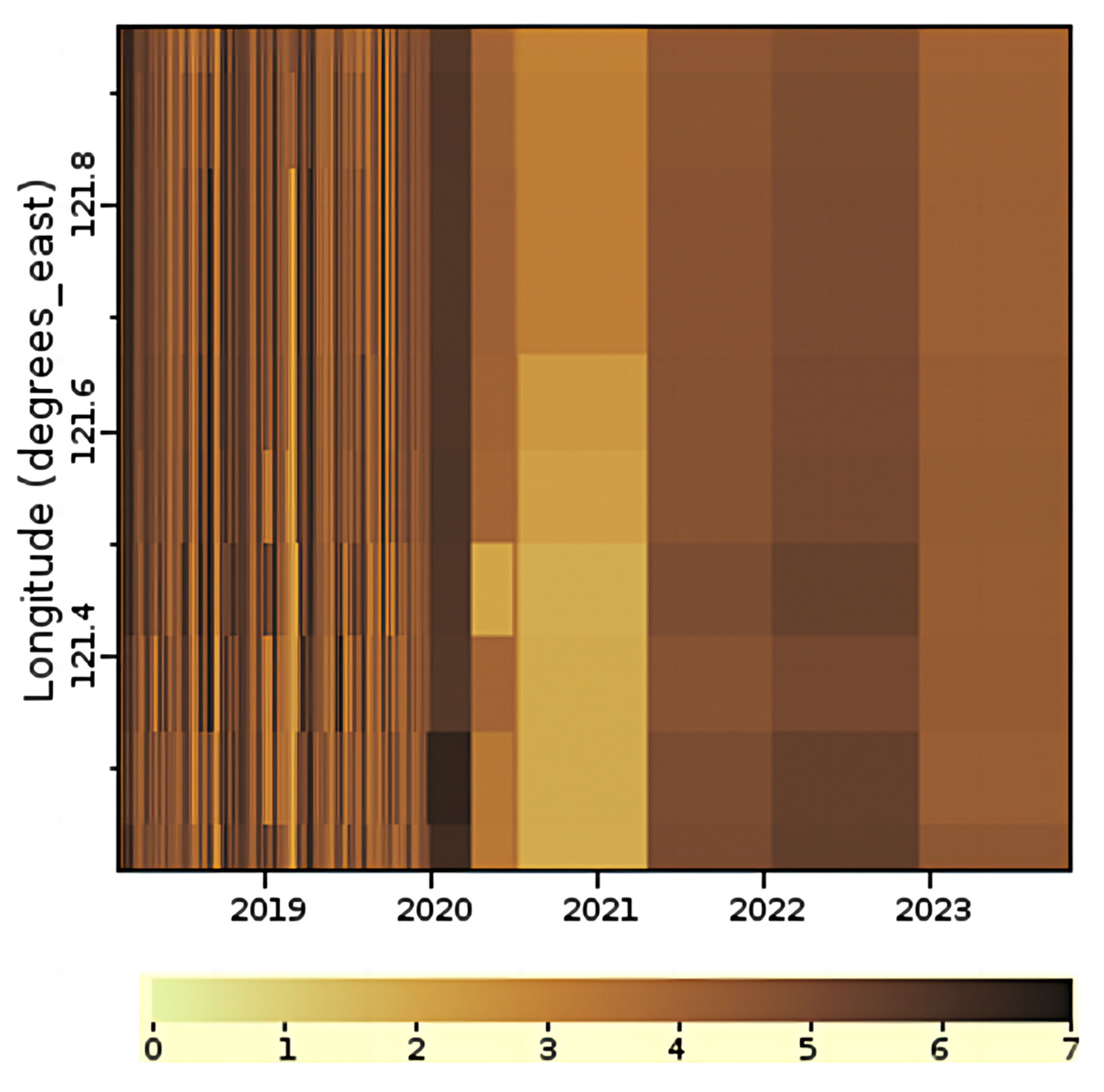
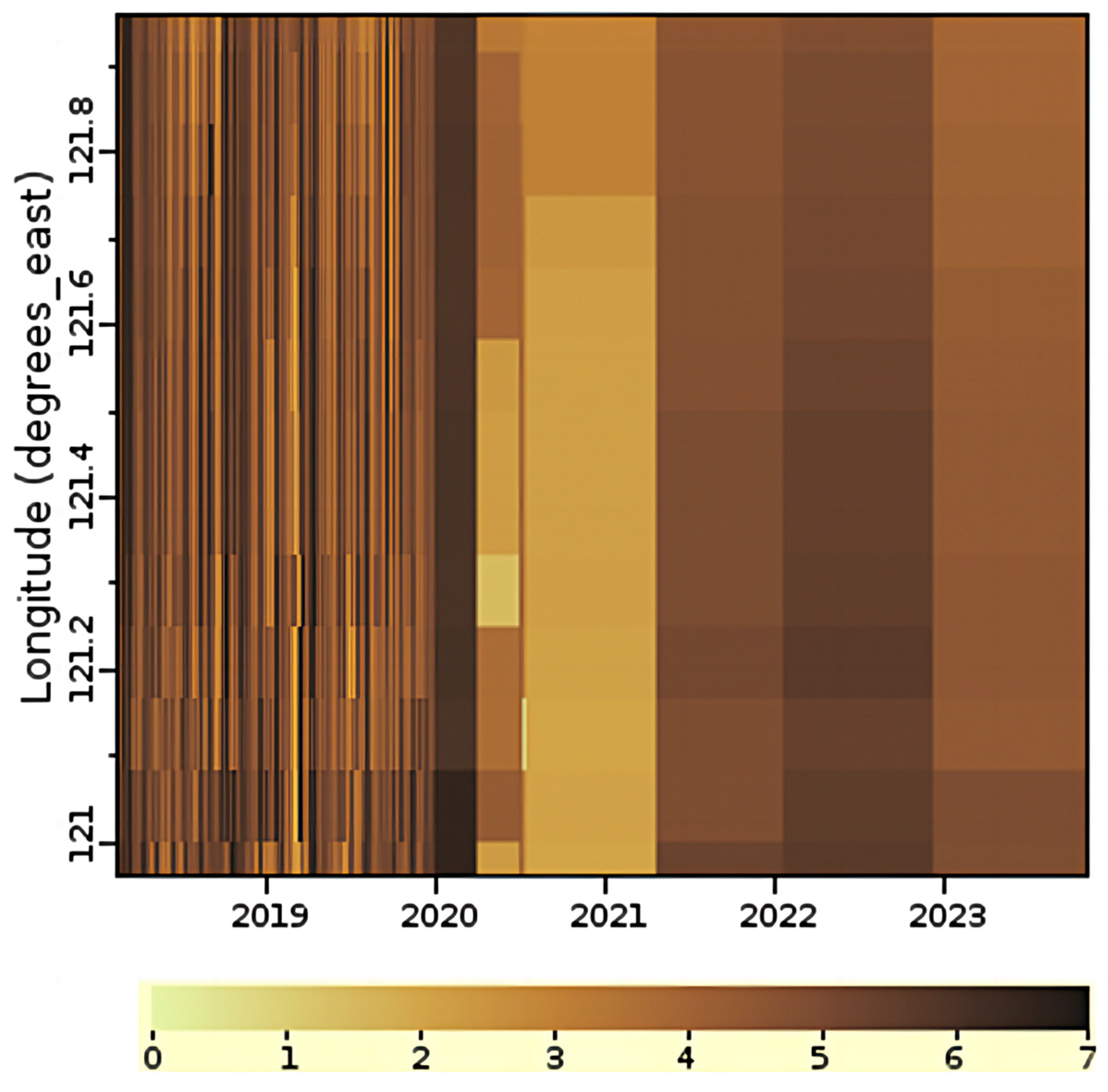
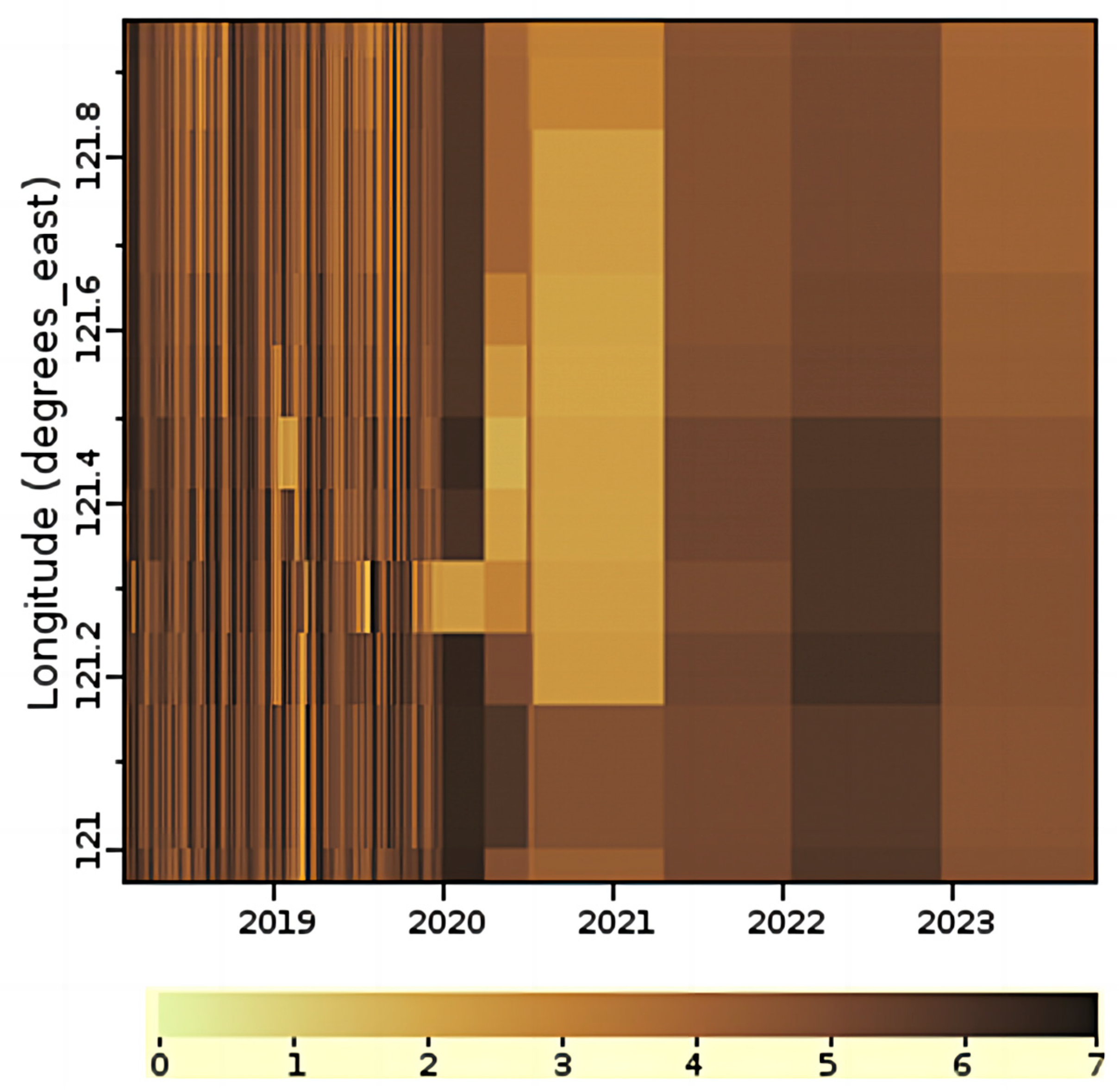
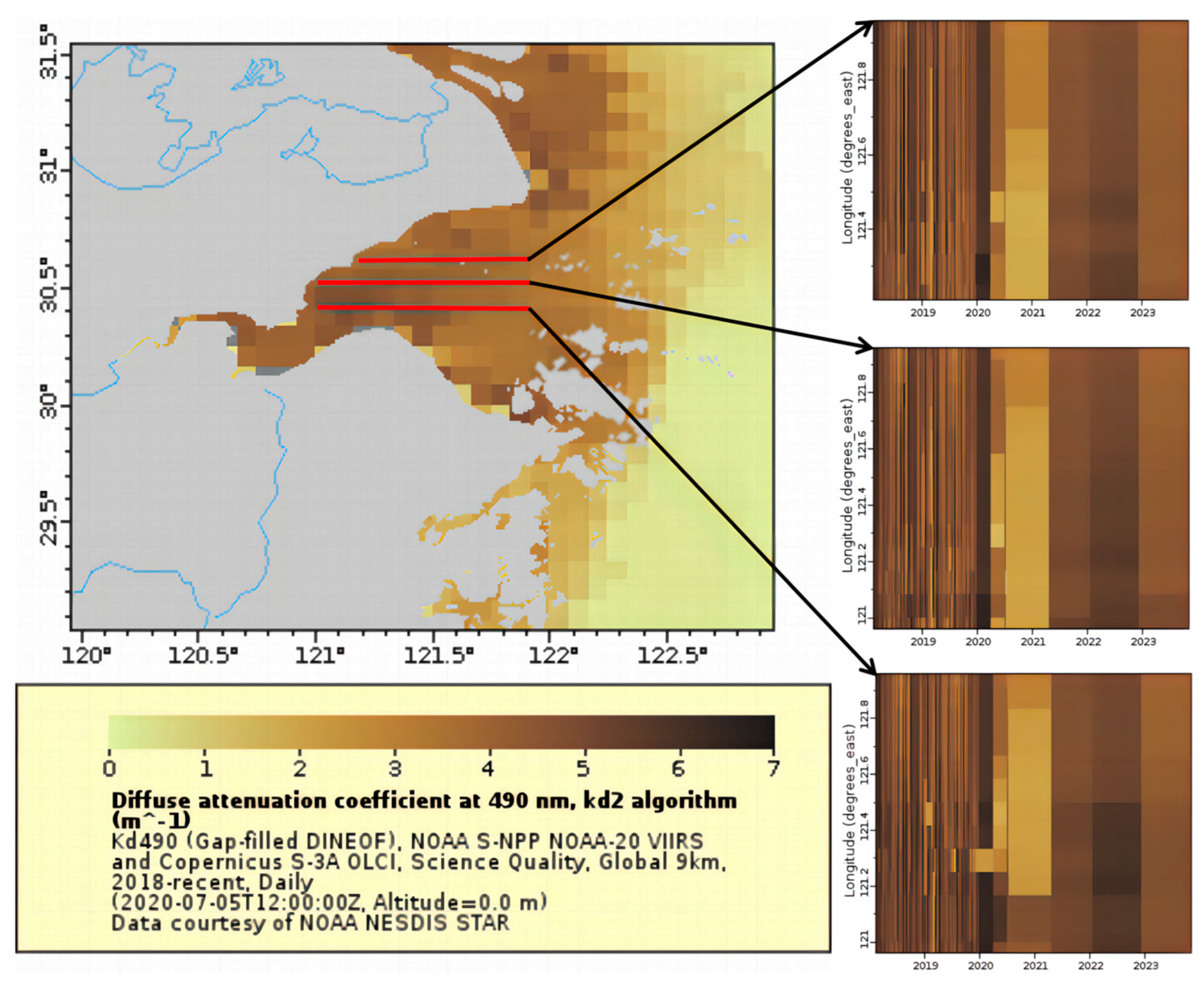
The left portion of Figure 2 shows the spatial distribution of Kd(490) in Hangzhou Bay on a given day. The 3 subplots in the right portion of the figure illustrate the variation of kd(490) with longitude and time at 3 given latitudes. Their enlarged figures are shown as Figure A1, Figure A2 and Figure A3 in Appendix A, where specific latitudes and longitudes are noted. The period of analysis is from February 2018 to October 2023. The Hangzhou Bay exhibits a high turbidity level, with Kd(490) varying spatially and temporally between 4 and 6 m−1. We select 20 study areas in Hangzhou Bay, and the locations, along with the daily mean Kd(490) values for each area, are shown in Figure 3 and Figure 4. It is pertinent to mention that the specific latitude and longitude data for the 20 study areas are presented in Table A1 in Appendix A, with the numbers 1–20.

3.1.2. Beibu Gulf

The Beibu Gulf is situated in the northwestern region of the South China Sea, with geographical coordinates ranging from 18.1 to 21.6° N and 105.6 to 109.7° E. It is bordered by the Leizhou Peninsula of Guangdong, Hainan Island, Guangxi Zhuang Autonomous Region, and Vietnam. The Gulf is abundant in marine biological resources and biodiversity [23], with a continental coastline of approximately 1595 km and an island coastline of up to 605 km.
The construction of the Beibu Gulf Economic Zone has been designated as a national strategy. As a result, the layout of heavy chemical industries and coastal industries are expanding in the region. However, this expansion poses significant challenges to the ecosystem of the Beibu Gulf, which raises widespread concerns about ecological security matters such as water security and environmental security in the region.
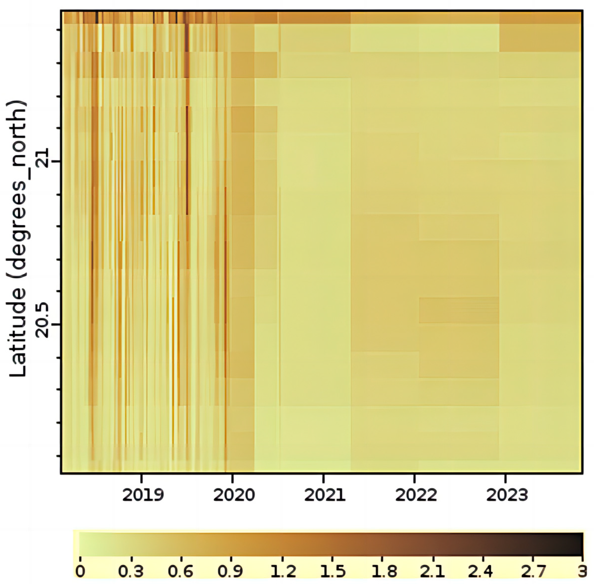
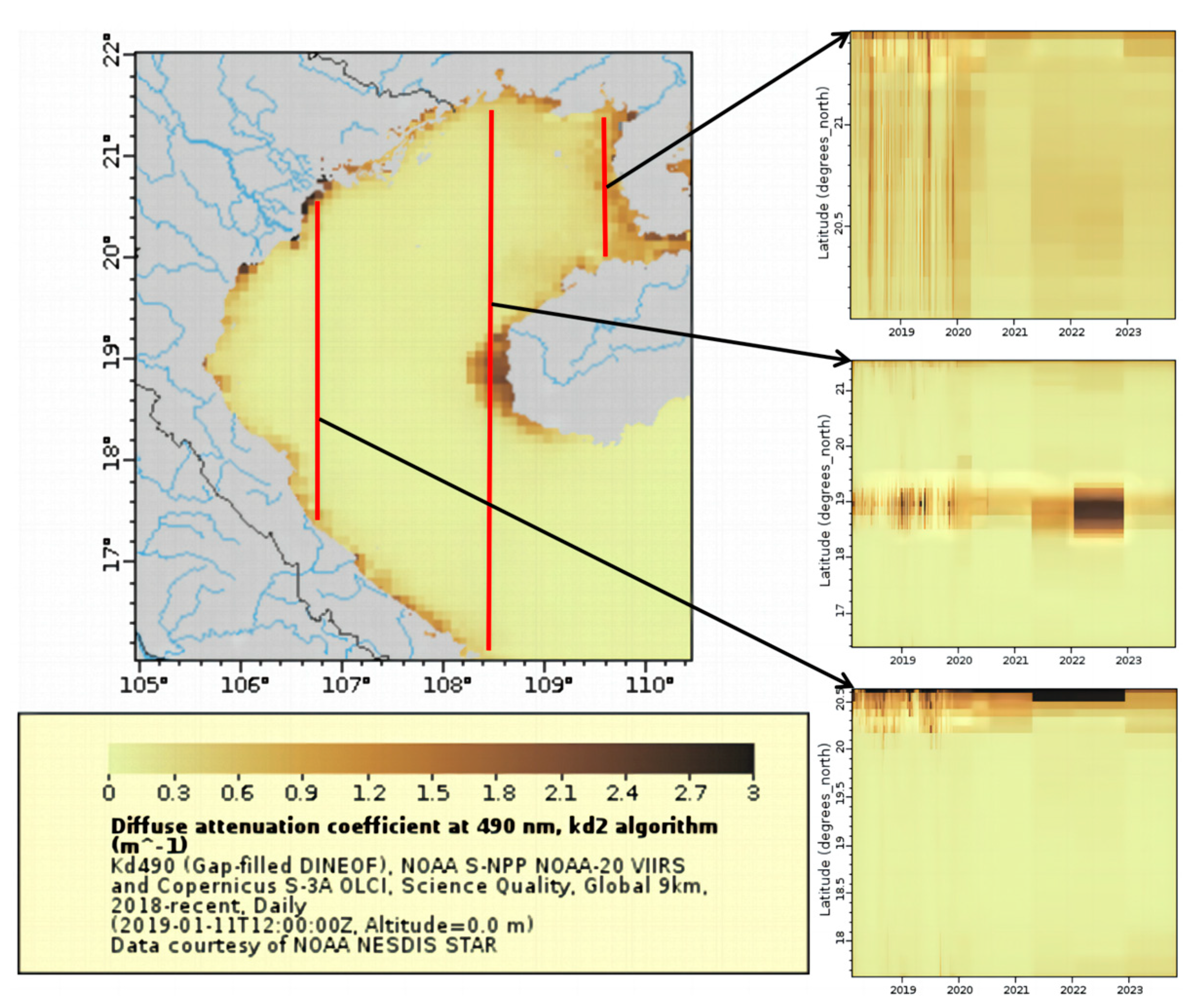
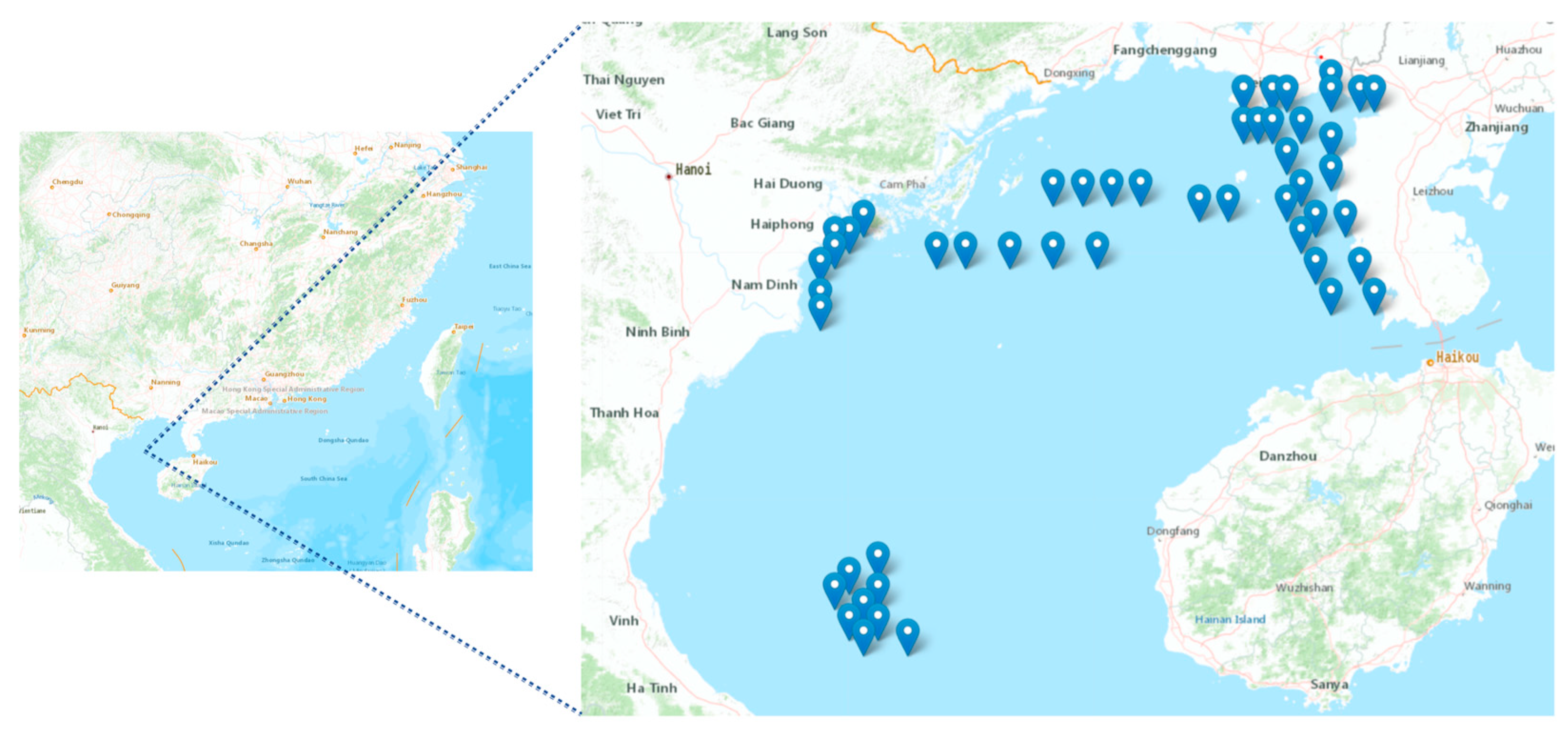
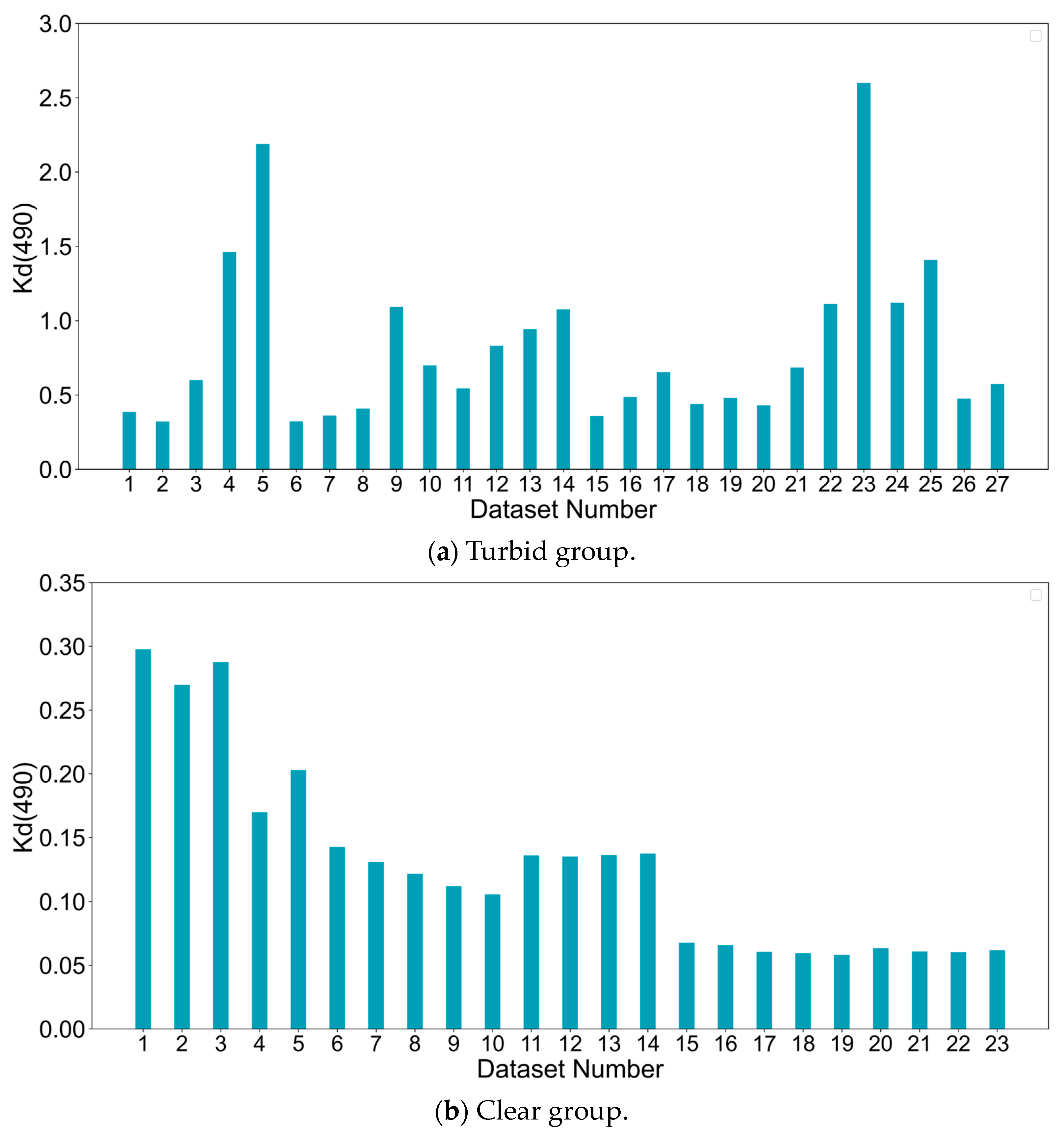
Similar to Figure 2, the left portion of Figure 5 shows the spatial distribution of Kd(490) in the Beibu Gulf on a given day. The 3 subplots in the right portion of the figure illustrate the variation of kd(490) with longitude and time at 3 given longitudes. Their enlarged figures and specific latitude and longitude information are shown as Figure A4, Figure A5 and Figure A6 in Appendix A. In the coastal waters of Beibu Gulf, the Kd(490) values are relatively high and vary in range from 0.5 to 2.8 m−1, indicating turbid waters. However, for the majority of the Beibu Gulf’s sea areas, the Kd(490) is below 0.3 m−1, indicating clear or relatively clear waters. Research on turbidity mechanisms in marine waters has shown that water turbidity is typically dominated by seasonal phytoplankton in waters with Kd(490) ≤ 0.3 m−1. In contrast, in waters with Kd(490) > 0.3 m−1, water turbidity is typically attributed to high sediment concentration loads due to various physical processes, such as sediment resuspension and river runoff [14]. Using Kd(490) = 0.3 m−1 as a threshold, we can ascertain the turbidity mechanisms of marine waters, as well as the degree of turbidity. Consequently, this study classifies 50 selected areas in the Beibu Gulf into two groups based on the daily mean Kd(490) = 0.3 m−1, i.e., the Beibu Gulf turbid group and the Beibu Gulf clear group. Figure 6 and Figure 7 show the location and daily mean Kd(490) for each study area. The specific latitude and longitude information for the 50 study areas is presented in Table A1 of Appendix A, with numbers 21–70.

3.2. Experimental Framework

The basic framework of the diffuse attenuation coefficient prediction experiment includes data preprocessing, data splitting, model training, model evaluation, and result analysis, as shown in Figure 8.
  • Data preprocessing: The global daily gap-free Kd(490) product used in this study covers the period from 9 February 2018 to 2 October 2023. The daily global Kd(490) data products are sampled based on the selected study areas. The time-series datasets for Kd(490) are obtained for each study area. The datasets are categorized into 3 groups based on the area location and daily mean Kd(490), i.e., the Hangzhou Bay dataset group, the Beibu Gulf turbid dataset group, and the Beibu Gulf clear dataset group. To address missing values in individual datasets, we use temporal linear interpolation. Additionally, we standardize the time-series data to facilitate model training.
  • Data splitting: In this study, we divide the training, validation set, and test set according to the ratio of 7:1:2. The length of the test set spans over a year, which enhances the reliability of the test results to some extent.
  • Model training: The RSIKP, ANN, CNN, GRU, LSTM-RNN, and LSTM models are analyzed and compared on the 3 dataset groups mentioned above at 15-day, 30-day, and 60-day prediction steps. It is conducted to identify the model that demonstrates optimal performance.
  • Model evaluation: Mean Absolute Error (MAE), Mean Square Error (MSE), and Mean Absolute Percentage Error (MAPE) are commonly used error evaluation metrics. MAE represents the real error between actual values and predicted values and is solely dependent on the data size. MSE guarantees that each term is positive and possesses differentiability. MAPE, which is expressed as a percentage, serves as a valuable metric for comparing predictions across various proportions. The 3 error metrics are expressed as
    M A E = 1 N i = 1 N | K i K ^ i |
    M S E = 1 N i = 1 N ( K i K ^ i ) 2
    M A P E = 100 % N i = 1 N | K i K ^ i K i |
    where K i is the i-th actual Kd(490), K ^ i is the i-th predicted Kd(490), and N is the total number of predicted points.
  • Results analysis: We visualized the error metrics of each model on different dataset groups. We could then more intuitively compare and analyze the performance of the models. In addition, we analyzed the variation in prediction performance of models as the prediction step increased.

4. Results and Discussion

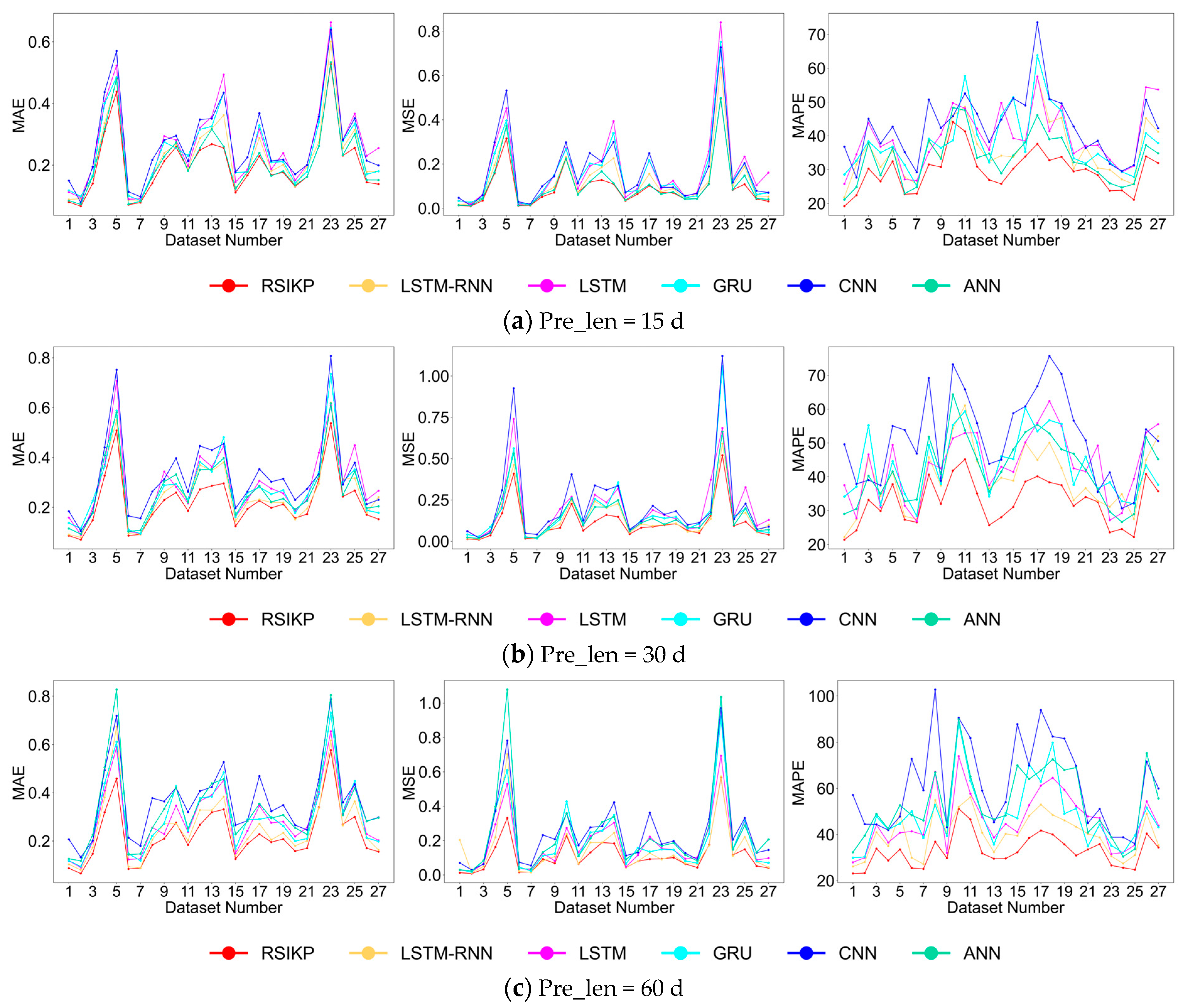
This study systematically evaluates the prediction performance of RSIKP and five other common prediction models by comparing and analyzing their error metrics on the Hangzhou Bay dataset group, the Beibu Gulf turbid dataset group, and the Beibu Gulf clear dataset group. In the experiments, we set different prediction step lengths (pre_len) at 15 days (15 d), 30 days (30 d), and 60 days (60 d). Table 2, Table 3 and Table 4 summarize the mean error metrics of all models on the three dataset groups, and the best results are shown in bold. In addition, we visualize the comparative results of the error metrics on each dataset through the line plots (refer to Figure 9, Figure 10 and Figure 11).

4.1. Analysis of Error Metrics

In Hangzhou Bay’s highly turbid waters, RSIKP demonstrates exceptional prediction performance. The mean values for MAE, MSE, and MAPE are 0.5391, 0.4637, and 13.7546, respectively. These metrics represent the most favorable outcomes among all models. Furthermore, as depicted in Figure 9, the error line of RSIKP (labeled in red) gradually diverges from the error lines of other models as the prediction step increases. The observation suggests that RSIKP has a growing advantage in prediction performance as the prediction step increases.
When pre_len = 15 d, the error metrics of ANN on individual datasets are similar to those of RSIKP. However, the mean values of MAE, MSE, and MAPE of RSIKP are significantly better than those of ANN. Out of the 20 datasets, RSIKP outperforms ANN in terms of MAPE on 18 datasets. Javier García-Alba and Amir Hamzeh Haghiabi et al. [6,24] used ANN for water quality prediction and had better prediction results. The ANN exhibits strong nonlinear modeling abilities due to the inclusion of the Rectified Linear Unit (ReLU). However, compared to RSIKP, ANN has limitations in comprehensively and centrally capturing the variation features of Kd(490) due to inherent structural constraints. And it tends to over-adapt to noise and subtle features in the training data, which makes it difficult to generalize to new data and results in prediction biases. In RSIKP, the Multi-head self-attention mechanism allows for a thorough extraction of features from the Kd(490) time series across multiple dimensions. Therefore, RSIKP can more accurately capture the variation features of Kd(490) induced by natural or anthropogenic events. Additionally, the sparsity of self-attention allows the RSIKP to focus on capturing more critical features of Kd(490) variations. Due to its comprehensiveness and precision in feature extraction, RSIKP demonstrates excellent performance in short-term and mid-term prediction.
When pre_len = 30 d and pre_len = 60 d, the overall prediction performance of LSTM-RNN is slightly inferior to that of RSIKP. However, it is noteworthy that RSIKP outperforms LSTM-RNN in three error metrics on all 20 datasets. L Kumar et al. [1] applied LSTM-RNN in turbidity prediction in Hong Kong waters. The model effectively addresses the issues of gradient vanishing and exploding in RNN by introducing LSTM structure and can better capture time dependencies. However, the recurrent structure and dynamic decoding structure of LSTM-RNN result in lower computational efficiency and persistent error accumulation. In contrast, RSIKP has lower computational complexity and can avoid the problem of error accumulation with its ProbSparse self-attention mechanism and generative decoding structure. Therefore, compared to LSTM-RNN, RSIKP demonstrates superior efficiency in long-sequence prediction and achieves higher accuracy.
The LSTM and GRU, two crucial variants of RNNS, both demonstrate a remarkable ability to effectively capture long-term dependencies when dealing with time-series data. As a result, their prediction performance exceeds that of ANN and CNN when pre_len = 60 d. LSTM is constructed by three gate structures, i.e., the input gate, the forget gate, and the output gate. And the cell state introduced in LSTM preserves long-term information in the Kd(490) time series better. GRU is composed of two gate structures, i.e., the update gate and the reset gate. It demonstrates superior prediction efficiency due to its simple structure. However, the merging of the cell state and hidden state into a single state in GRU may result in the loss of long-term information. Therefore, the prediction performance of GRU is inferior to that of LSTM when pre_len = 60 d. Additionally, among the six models, the CNN demonstrates relatively poor predictive performance. Although it can capture some local features in time series, its insufficient consideration of temporal dependencies still results in sub-optimal performance in temporal prediction.
On the Beibu Gulf turbid dataset group, we observe distinctions between RSIKP and other models, which are similar to those observed in the Hangzhou Bay dataset group. Among all models, RSIKP shows the best performance on all three error metrics. And it is noteworthy that the error metrics of all models exhibit an increase compared to those on the Hangzhou Bay dataset group. In response to this phenomenon, we conduct a detailed analysis of this dataset group. The study areas corresponding to the Beibu Gulf turbid dataset group are located near the coastline, characterized by high population density and industrial development within the coastal regions. The frequent anthropogenic events impact the variations of Kd(490) in coastal waters, resulting in a high degree of instability and stochasticity in the corresponding Kd(490) time series. This makes predictions more difficult. However, RSIKP still maintains robust prediction performance with a mean prediction accuracy of nearly 70% on the Beibu Gulf turbid datasets, which are characterized by highly complex features. Therefore, it can be concluded that RSIKP demonstrates outstanding adaptability and reliability in complex and unstable marine environments and has stronger robustness against variations in datasets. In spite of the complexity of the factors affecting Kd(490), an important indicator of marine water quality, RSIKP maintains good predictive accuracy and reliability. This finding provides substantial support for marine water quality predictions.
On the Beibu Gulf clear dataset group, RSIKP still demonstrates outstanding prediction performance. Our analysis reveals a clear seasonality in the time series of Kd(490) in this group. According to Shi Wei et al.’s study on turbidity mechanisms in marine waters, the variation of Kd(490) is dominated by seasonal phytoplankton blooms in waters with Kd(490) ≤ 0.3 m−1 [15]. Thus, it is evident that seasonal features dominate among the various features. The RSIKP can accurately capture the seasonal features in the variations of Kd(490) due to its centralized learning features and deep network structure. Apart from seasonality, other factors such as ocean currents and wind [25] also affect the variations of Kd(490). The RSIKP can extract these underlying features through its robust multi-dimension feature extraction capability. Therefore, the RSIKP still demonstrates superior prediction performance compared to other models in time series with clear seasonality.

4.2. Effect of Prediction Step on Performance

After analyzing the experimental results on the three dataset groups, it is observed that the mean error metric of ANN is second only to RSIKP when pre_len = 15 d. The prediction performance of LSTM-RNN is second only to RSIKP when pre_len = 30 d and pre_len = 60 d. For the three prediction models that perform prominently, we further compare and analyze the changes in their error metrics as the prediction step increases. To quantify the extent of the changes in the error metrics, we introduce three metrics, i.e., GMAE, GMSE, and GMAPE. These metrics indicate the rate of change in three error metrics as the prediction step increases. The expressions for three metrics are as follows:
G M A E = ( M A E pre _ l e n 2 M A E p r e _ l e n 1 ) M A E pre _ l e n 1 100 %
G M S E = ( M S E pre _ l e n 2 M S E p r e _ l e n 1 ) M S E pre _ l e n 1 100 %
G M A P E = ( M A P E pre _ l e n 2 M A P E p r e _ l e n 1 ) M A P E pre _ l e n 1 100 %
where pre_len1 and pre_len2 represent two different prediction steps, with pre_len2 being greater than pre_len1. For example, we use Equation (10) with pre_len1 = 15 d and pre_len2 = 30 d to calculate GMAE between prediction steps of 15 days and 30 days (15–30 d). Table 5 and Figure 12 illustrate the trend in the error metrics of the three models on the three dataset groups as the prediction step increases.
Upon analyzing Figure 12 and Table 5, it is evident that the error metrics of RSIKP show only a slight upward trend as the prediction step increases. The average MAPE of RSIKP only increases by 13.2% when pre_len is increased from 15 d to 60 d, maintaining satisfactory prediction performance. Notably, as pre_len increases from 30 d to 60 d, the MAE and MSE metrics of RSIKP exhibit a marginal decrease in the Hangzhou Bay dataset group and the Beibu Gulf clear dataset group. This observation further confirms the high applicability of RSIKP in long-time-series prediction. In contrast, while the prediction performance of ANN can approach that of RSIKP when pre_len = 15 d, the three error metrics of ANN increase significantly as the prediction step increases. Specifically, the average MAPE of ANN increases by 67.7% when pre_len increases from 15 d to 60 d, indicating a substantial degradation in prediction performance. Therefore, It can be concluded that ANN is only suitable for the shorter time-series prediction. The error metrics of LSTM-RNN exhibit a relatively small change rate compared to ANN. However, the change rate in error metrics of LSTM-RNN is significantly higher than that of RSIKP on the Hangzhou Bay dataset group and the Beibu Gulf clear dataset group. Furthermore, the overall error of LSTM-RNN is significantly higher than that of RSIKP. The above analysis demonstrates the clear advantages of RSIKP in long time-series prediction.

5. Conclusions and Prospects

The diffuse attenuation coefficient (Kd) is a crucial apparent optical parameter that reflects the rate of light attenuation in the water. It serves as an important indicator of water quality and turbidity. This paper innovatively applies RSIKP to the prediction of Kd in marine waters. Multi-dataset prediction experiments are conducted at different steps for 20 areas in Hangzhou Bay and 50 areas in the Beibu Gulf. And we evaluate the performance of six prediction models using three error metrics. The results show that RSIKP achieves the optimal performance on three dataset groups. This model outperforms the other five models by averages of 20.6%, 31.1%, and 22.9% on MAE, MSE, and MAPE, which demonstrates its strong prediction potential in the prediction of marine waters’ Kd. Furthermore, we analyzed the effect of the prediction step on performance for high-performing prediction models, i.e., RSIKP, ANN, and LSTM-RNN. The MAPE of RSIKP increased by only 13.2% on average when the prediction step increased from 15 days to 60 days. In contrast, both ANN and LSTM-RNN experience a much larger increase in MAPE, with an average increase of 67.7% and 21.6%, respectively. This statement proves that the RSIKP is capable of maintaining excellent performance in long-time-series prediction. The RSIKP proposed in this study achieves accurate prediction of the variations of Kd(490) in marine water, a key indicator of water quality. In particular, RSIKP demonstrates superior performance in the 60-day long-term prediction compared to other prediction models, enabling the monitoring of water quality trends over a longer period of time in the future. This augments the ability to monitor and respond to variations in seawater quality, which promotes the optimization of environmental conservation measures in the coastal region.
It is our hope that researchers will apply remote sensing data and neural network models to water quality prediction with greater frequency to address the high cost and large regional constraints on water quality prediction. This will enhance the maturity of the application of remote sensing data in water quality prediction. Additionally, the improvement of the precision of water quality prediction will provide more scientific and reliable guidance for marine water quality management and environmental management in coastal areas. Finally, considering the outstanding performance of RSIKP, we also plan to integrate it into water quality prediction in specific waters. Our aim is to make practical contributions to water quality management.

Author Contributions

R.C. investigation, methodology, code, data curation, visualization, writing—original draft preparation; M.H. funding acquisition, supervision, writing—review and editing; X.G. conceptualization, supervision, writing—review and editing; M.K.I. writing—review and editing; C.W. writing—review and editing. All authors have read and agreed to the published version of the manuscript.

Funding

This research was funded by the Primary Research and Development Plan of Zhejiang Province (2023C03014), the “Pioneer” and “Leading Goose” R&D Program of Zhejiang (2024C03033) and the Fundamental Research Funds for the Provincial Universities of Zhejiang (GK239909299001-045).

Data Availability Statement

Conflicts of Interest

The authors declare no conflicts of interest.

Appendix A

Table A1. The specific latitude and longitude of the study areas in Hangzhou Bay and Beibu Gulf.
Sea LocationNumberLatitudeLongitude
Hangzhou Bay130.792° N121.875° E
230.542° N121.875° E
330.292° N121.875° E
430.125° N121.875° E
530.792° N121.708° E
630.625° N121.708° E
730.458° N121.708° E
830.292° N121.708° E
930.125° N121.708° E
1030.708° N121.542° E
1130.541° N121.542° E
1230.292° N121.542° E
1330.708° N121.458° E
1430.458° N121.458° E
1530.625° N121.375° E
1630.375° N121.375° E
1730.625° N121.292° E
1830.542° N121.208° E
1930.458° N121.042° E
2030.291° N120.875° E
Beibu Gulf2121.375° N109.125° E
2221.375° N109.292° E
2321.375° N109.375° E
2421.375° N109.625° E
2521.375° N109.792° E
2621.375° N109.875° E
2721.208° N109.125° E
2821.208° N109.208° E
2921.208° N109.292° E
3021.208° N109.458° E
3120.792° N108.875° E
3220.792° N109.042° E
3320.792° N109.375° E
3420.542° N107.375° E
3520.542° N107.542° E
3620.542° N107.792° E
3720.542° N108.042° E
3820.542° N108.292° E
3921.458° N109.625° E
4021.125° N109.625° E
4120.958° N109.625° E
4220.708° N109.708° E
4320.458° N109.792° E
4420.292° N109.875° E
4521.042° N109.375° E
4620.875° N109.458° E
4720.708° N109.542° E
4820.625° N109.458° E
4920.458° N109.542° E
5020.292° N109.625° E
5120.708° N106.958° E
5220.625° N106.875° E
5320.625° N106.792° E
5420.542° N106.792° E
5520.458° N106.708° E
5620.292° N106.708° E
5720.208° N106.708° E
5820.875° N108.042° E
5920.875° N108.208° E
6020.875° N108.375° E
6120.875° N108.542° E
6218.708° N106.792° E
6318.542° N106.875° E
6418.625° N106.958° E
6518.708° N107.042° E
6618.458° N107.208° E
6718.792° N106.875° E
6818.875° N107.042° E
6918.542° N107.042° E
7018.458° N106.958° E
Figure A1. Spatial and temporal variations of Kd(490) in Hangzhou Bay waters (Lat: 30.63° N, Lon: 121.21–121.96° E).
Water 16 01279 g0a1
Figure A2. Spatial and temporal variations of Kd(490) in Hangzhou Bay waters (Lat: 30.54° N, Lon: 120.96–121.96° E).
Water 16 01279 g0a2
Figure A3. Spatial and temporal variations of Kd(490) in Hangzhou Bay waters (Lat: 30.46° N, Lon: 120.96–121.96° E).
Water 16 01279 g0a3
Figure A4. Spatial and temporal variations of Kd(490) in Beibu Gulf waters (Lat: 20.04–21.46° N, Lon: 109.46° E).
Water 16 01279 g0a4
Figure A5. Spatial and temporal variations of Kd(490) in Beibu Gulf waters (Lat: 16.38–21.54° N, Lon: 108.46° E).
Water 16 01279 g0a5
Figure A6. Spatial and temporal variations of Kd(490) in Beibu Gulf waters (Lat: 17.63–20.63° N, Lon: 106.71° E).
Water 16 01279 g0a6

References

  1. Kumar, L.; Afzal, M.S.; Ahmad, A. Prediction of water turbidity in a marine environment using machine learning: A case study of Hong Kong. Reg. Stud. Mar. Sci. 2022, 52, 102260. [Google Scholar] [CrossRef]
  2. Ahmed, A.N.; Othman, F.B.; Afan, H.A.; Ibrahim, R.K.; Fai, C.M.; Hossain, M.S.; Ehteram, M.; Elshafie, A. Machine learning methods for better water quality prediction. J. Hydrol. 2019, 578, 124084. [Google Scholar] [CrossRef]
  3. Noori, N.; Kalin, L.; Isik, S. Water quality prediction using SWAT-ANN coupled approach. J. Hydrol. 2020, 590, 125220. [Google Scholar] [CrossRef]
  4. Dritsas, E.; Trigka, M. Efficient Data-Driven Machine Learning Models for Water Quality Prediction. Computation 2023, 11, 16. [Google Scholar] [CrossRef]
  5. García-Alba, J.; Bárcena, J.F.; Ugarteburu, C.; García, A. Artificial neural networks as emulators of process-based models to analyse bathing water quality in estuaries. Water Res. 2019, 150, 283–295. [Google Scholar] [CrossRef] [PubMed]
  6. Wu, Y.; Yang, Y.; Nishiura, H.; Saitoh, M. Deep learning for epidemiological predictions. In Proceedings of the 41st International ACM SIGIR Conference on Research and Development in Information Retrieval, Ann Arbor, MI, USA, 8–12 July 2018; pp. 1085–1088. [Google Scholar]
  7. Zhou, J.; Wang, Y.; Xiao, F.; Wang, Y.; Sun, L. Water quality prediction method based on IGRA and LSTM. Water 2018, 10, 1148. [Google Scholar] [CrossRef]
  8. Arepalli, P.G.; Akula, M.; Kalli, R.S.; Kolli, A.; Popuri, V.P.; Chalichama, S. Water quality prediction for salmon fish using gated recurrent unit (GRU) model. In Proceedings of the 2022 Second International Conference on Computer Science, Engineering and Applications (ICCSEA), Gunupur, India, 8 September 2022; pp. 1–5. [Google Scholar]
  9. Liu, X.; Wang, M. Global daily gap-free ocean color products from multi-satellite measurements. Int. J. Appl. Earth Obs. Geoinf. 2022, 108, 102714. [Google Scholar] [CrossRef]
  10. Lund-Hansen, L.C. Diffuse attenuation coefficients Kd (PAR) at the estuarine North Sea–Baltic Sea transition: Time-series, partitioning, absorption, and scattering. Estuar. Coast. Shelf Sci. 2004, 61, 251–259. [Google Scholar] [CrossRef]
  11. Wang, W.; Zhao, J. Variation of Diffuse Attenuation Coefficient of Downwelling Irradiance in the Arctic Ocean. Acta Oceanol. Sin. 2014, 33, 53–62. [Google Scholar] [CrossRef]
  12. Prieur, L.; Sathyendranath, S. An optical classification of coastal and oceanic waters based on the specific spectral absorption curves of phytoplankton pigments, dissolved organic matter, and other particulate materials. Limnol. Oceanogr. 1981, 26, 671–689. [Google Scholar] [CrossRef]
  13. Pope, R.M.; Fry, E.S. Absorption spectrum (380–700 nm) of pure water. II. Integrating cavity measurements. Appl. Opt. 1997, 36, 8710–8723. [Google Scholar] [CrossRef] [PubMed]
  14. Shi, W.; Wang, M. Characterization of global ocean turbidity from Moderate Resolution Imaging Spectroradiometer ocean color observations. J. Geophys. Res. Ocean. 2010, 115, C11022. [Google Scholar] [CrossRef]
  15. Rodríguez-López, L.; González-Rodríguez, L.; Duran-Llacer, I.; García, W.; Cardenas, R.; Urrutia, R. Assessment of the Diffuse Attenuation Coefficient of Photosynthetically Active Radiation in a Chilean Lake. Remote Sens. 2022, 14, 4568. [Google Scholar] [CrossRef]
  16. Bardaji, R.; Sánchez, A.-M.; Simon, C.; Wernand, M.R.; Piera, J. Estimating the underwater diffuse attenuation coefficient with a low-cost instrument: The KdUINO DIY buoy. Sensors 2016, 16, 373. [Google Scholar] [CrossRef] [PubMed]
  17. Vaswani, A.; Shazeer, N.; Parmar, N.; Uszkoreit, J.; Jones, L.; Gomez, A.N.; Kaiser, Ł.; Polosukhin, I. Attention is all you need. In Proceedings of the 31st Annual Conference on Neural Information Processing Systems (NIPS 2017), Long Beach, CA, USA, 4–9 December 2017. [Google Scholar]
  18. Zhou, H.; Zhang, S.; Peng, J.; Zhang, S.; Li, J.; Xiong, H.; Zhang, W. Informer: Beyond efficient transformer for long sequence time-series forecasting. In Proceedings of the Thirty-Fifth AAAI Conference on Artificial Intelligence, Virtual, 2–9 February 2021. [Google Scholar]
  19. Rahhal, M.M.A.; Bazi, Y.; Alsharif, N.A.; Bashmal, L.; Alajlan, N.; Melgani, F. Multilanguage Transformer for Improved Text to Remote Sensing Image Retrieval. IEEE J. Sel. Top. Appl. Earth Obs. Remote Sens. 2022, 15, 9115–9126. [Google Scholar] [CrossRef]
  20. Bi, C.; Ren, P.; Yin, T.; Zhang, Y.; Li, B.; Xiang, Z. An Informer Architecture-Based Ionospheric foF2 Model in the Middle Latitude Region. IEEE Geosci. Remote Sens. Lett. 2022, 19, 1005305. [Google Scholar] [CrossRef]
  21. Fang, Z.; Feng, T.; Qin, G.; Meng, Y.; Zhao, S.; Yang, G.; Wang, L.; Sun, W. Simulations of water pollutants in the Hangzhou Bay, China: Hydrodynamics, characteristics, and sources. Mar. Pollut. Bull. 2024, 200, 116140. [Google Scholar] [CrossRef]
  22. Qinghui, M.; Lin, W.; Zhihua, M. Preliminary study on the application of HJ CCD imagery to water quality assessment for Hangzhou Bay. Guangxi Sci. 2015, 22, 322–328. [Google Scholar]
  23. Luo, Z.L.; Yang, C.P.; Wang, L.M.; Liu, Y.; Shan, B.B.; Liu, M.T.; Chen, C.; Guo, T.; Sun, D. Relationships between Fish Community Structure and Environmental Factors in the Nearshore Waters of Hainan Island, South China. Diversity 2023, 15, 901. [Google Scholar] [CrossRef]
  24. Haghiabi, A.H.; Nasrolahi, A.H.; Parsaie, A. Water quality prediction using machine learning methods. Water Qual. Res. J. Can. 2018, 25, 23–28. [Google Scholar] [CrossRef]
  25. Qiu, Z.; Wu, T.; Su, Y. Retrieval of diffuse attenuation coefficient in the China seas from surface reflectance. Opt. Express 2013, 21, 15287–15297. [Google Scholar] [CrossRef] [PubMed]
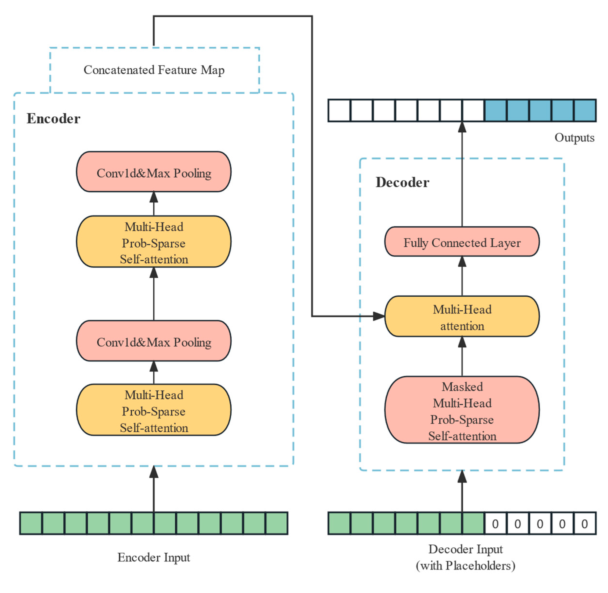
Figure 1. The structure of Informer.
Water 16 01279 g001
Figure 2. Spatial and temporal distribution of Kd(490) in Hangzhou Bay.
Water 16 01279 g002
Figure 3. Location of study areas in Hangzhou Bay.
Water 16 01279 g003
Figure 4. Daily mean Kd(490) of each study area in Hangzhou Bay.
Water 16 01279 g004
Figure 5. Spatial and temporal distribution of Kd(490) in Beibu Gulf.
Water 16 01279 g005
Figure 6. Location of study areas in Beibu Gulf.
Water 16 01279 g006
Figure 7. Daily mean Kd(490) of each study area in Beibu Gulf. (a) represents turbid group. (b) represents clear group.
Water 16 01279 g007
Figure 8. Framework of the experiment.
Water 16 01279 g008
Figure 9. Error metrics for all models on each dataset of Hangzhou Bay group. (a) pre_len = 15 d. (b) pre_len = 30 d. (c) pre_len = 60 d.
Water 16 01279 g009
Figure 10. Error metrics for all models on each dataset of the Beibu Gulf turbid group. (a) pre_len = 15 d. (b) pre_len = 30 d. (c) pre_len = 60 d.
Water 16 01279 g010
Figure 11. Error metrics for all models on each dataset of the Beibu Gulf clear group. (a) pre_len = 15 d. (b) pre_len = 30 d. (c) pre_len = 60 d.
Water 16 01279 g011
Figure 12. Variations in error metrics of RSIKP, ANN, and LSTM-RNN as the prediction step increases on 3 dataset groups. (a) Hangzhou Bay dataset group. (b) Beibu Gulf turbid dataset group. (c) Beibu Gulf clear dataset group.
Water 16 01279 g012
Table 1. Parameters setting of RSIKP.
ParametersDescriptionValue
gpuGPUcuda1
lossloss function“mse”
patienceearly stopping patience3
inverseinverse of dataTrue
enc_inencoder input size1
dec_indecoder input size1
dec_outdecoder output size 1
n_headsnumbers of heads8
d_modelmodel dimension512
dropoutdropout0.05
batch_sizeBatch size32
enc_layerslayers of encoder2
dec_layerslayers of decoder1
seq_lengthsequence length15–90
lab_lengthlable length7–60
pre_lengthprediction length7–60
train_epochstrain epochs500
learning_rateleaning rate0.0001
Table 2. Mean error metrics for all models on the Hangzhou Bay dataset group.
pre_len
Model
RSIKPANNCNNGRULSTM-RNNLSTM
15 dMAE0.52190.53020.66150.64870.58080.6552
MSE0.44710.46040.71240.69120.55820.7147
MAPE13.070913.531016.781916.488514.837516.5615
30 dMAE0.55170.61070.72850.67950.61040.7061
MSE0.47630.59930.85110.74420.60360.7867
MAPE13.874215.640018.456617.480015.591518.0747
60 dMAE0.54370.74330.80870.73120.66290.7106
MSE0.46760.88451.03330.82730.69860.8046
MAPE14.318719.092120.721719.214617.293018.6928
The bold numbers indicate the lowest error value of all models.
Table 3. Mean error metrics for all models on the Beibu Gulf turbid dataset group.
pre_len
Model
RSIKPANNCNNGRULSTM-RNNLSTM
15 dMAE0.20230.21370.27400.25300.23170.2667
MSE0.09730.10460.16820.15780.12580.1733
MAPE29.597133.315742.695338.339135.809739.6464
30 dMAE0.22170.26870.32370.28120.25460.2922
MSE0.11320.15360.22340.18110.14040.1929
MAPE32.567342.234451.686643.473739.472143.6236
60 dMAE0.22620.33730.36350.30280.25880.2941
MSE0.11680.23720.24830.20000.15250.1815
MAPE32.948453.829461.927148.280340.190646.1878
The bold numbers indicate the lowest error value of all models.
Table 4. Mean error metrics for all models on the Beibu Gulf clear dataset group.
pre_len
Model
RSIKPANNCNNGRULSTM-RNNLSTM
15 dMAE0.02840.02950.03740.03400.03110.0346
MSE0.00380.00400.00630.00620.00480.0051
MAPE18.617619.645124.965922.234420.714722.9925
30 dMAE0.03240.03950.04890.03910.03550.0434
MSE0.00450.00630.00890.00570.00510.0081
MAPE22.124527.119134.142528.689125.338330.1258
60 dMAE0.03130.05320.06350.04260.03780.0426
MSE0.00390.00960.01260.00650.00590.0071
MAPE22.110039.391347.442631.325428.161930.0850
The bold numbers indicate the lowest error value of all models.
Table 5. The change rate in error metrics of RSIKP, ANN, and LSTM-RNN as the prediction step increases on 3 dataset groups.
Dataset GroupChange RateRSIKPANNLSTM-RNN
Hangzhou Bay15–30 dGMAE5.709915.18295.0964
GMSE6.531030.16948.1333
GMAPE6.145715.58645.0817
30–60 dGMAE−1.450121.71288.6009
GMSE−1.826647.588915.7389
GMAPE3.203822.072310.9130
15–60 dGMAE4.177040.192414.1357
GMSE4.585192.115625.1523
GMAPE9.546441.099016.5493
Beibu Gulf turbid15–30 dGMAE9.589725.73709.8835
GMSE16.341246.845111.6057
GMAPE10.035426.770310.2274
30–60 dGMAE2.029825.53031.6496
GMSE3.180254.42718.6182
GMAPE1.170227.45391.8203
15–60 dGMAE11.814157.838111.6962
GMSE20.0411126.768621.2242
GMAPE11.323161.573712.2338
Beibu Gulf clear15–30 dGMAE14.084533.898314.1479
GMSE18.421157.50006.2500
GMAPE18.836538.045122.3204
30–60 dGMAE−3.395134.68356.4789
GMSE−13.333352.381015.6863
GMAPE−0.065545.253011.1436
15–60 dGMAE10.211380.339021.5434
GMSE2.6316140.000022.9167
GMAPE18.7586100.514635.9513
Disclaimer/Publisher’s Note: The statements, opinions and data contained in all publications are solely those of the individual author(s) and contributor(s) and not of MDPI and/or the editor(s). MDPI and/or the editor(s) disclaim responsibility for any injury to people or property resulting from any ideas, methods, instructions or products referred to in the content.