
Using the Periodic Dynamics of Well Water Levels to Estimate Time Series Changes in Aquifer Parameters


Abstract
1. Introduction
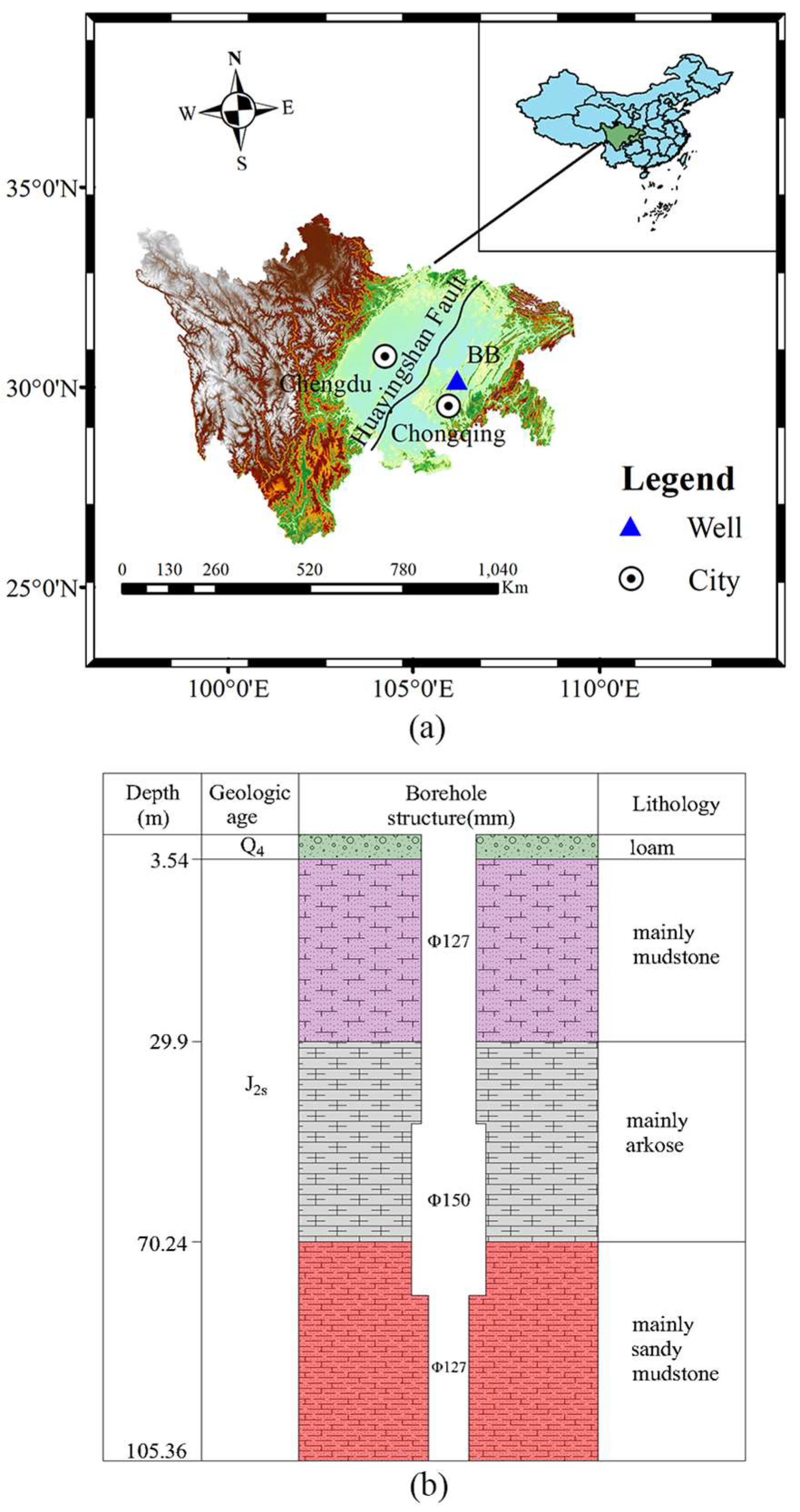
2. Observation Background and Data
3. Methods
3.1. Determination of Storage Coefficient
3.2. Determination of BKu
3.3. Calculation Theory of Horizontal Transmissivity and Leakage Coefficient
4. Results
5. Discussion
5.1. Verification of Results
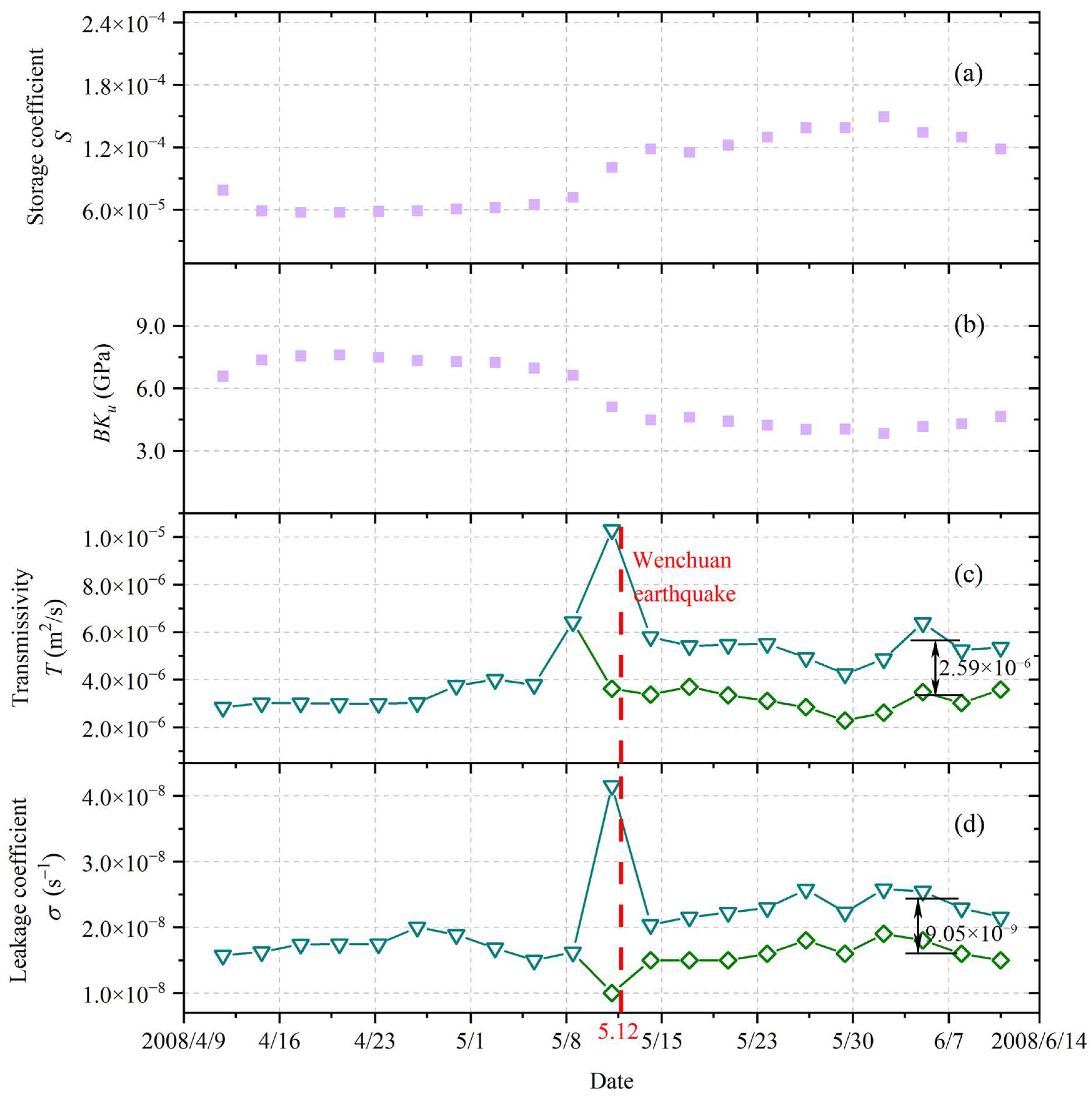
5.2. The Effects of Earthquakes
6. Conclusions
Supplementary Materials
Author Contributions
Funding
Data Availability Statement
Conflicts of Interest
References
- Manga, M. Origin of postseismic streamflow changes inferred from baseflow recession and magnitude-distance relations. Geophys. Res. Lett. 2001, 28, 2133–2136. [Google Scholar] [CrossRef]
- Carrigan, C.R.; King, G.C.P.; Barr, G.E.; Bixler, N.E. Potential for water-table excursions induced by seismic events at yucca mountain, nevada. Geology 1991, 19, 1157–1160. [Google Scholar] [CrossRef]
- Weeks, E.P. Barometric fluctuations in wells tapping deep unconfined aquifers. Water Resour. Res. 1979, 15, 1167–1176. [Google Scholar] [CrossRef]
- Van der Kamp, G.; Gale, J. Theory of earth tide and barometric effects in porous formations with compressible grains. Water Resour. Res. 1983, 19, 538–544. [Google Scholar] [CrossRef]
- Rojstaczer, S.; Riley, F.S. Response of the water level in a well to earth tides and atmospheric loading under unconfined conditions. Water Resour. Res. 1990, 26, 1803–1817. [Google Scholar] [CrossRef]
- Bredehoeft, J.D. Response of well-aquifer systems to Earth tides. J. Geophys. Res. 1967, 72, 3075–3087. [Google Scholar] [CrossRef]
- Hsieh, P.A.; Bredehoeft, J.D.; Farr, J.M. Determination of aquifer transmissivity from Earth tide analysis. Water Resour. Res. 1987, 23, 1824–1832. [Google Scholar] [CrossRef]
- Cooper, H.H., Jr.; Bredehoeft, J.D.; Papadopulos, I.S. Response of a finite-diameter well to an instantaneous charge of water. Water Resour. Res. 1967, 3, 263–269. [Google Scholar] [CrossRef]
- Liu, L.B.; Roeloffs, E.; Zheng, X.Y. Seismically induced water level fluctuations in the Wali well, Beijing, China. J. Geophys. Res.-Solid Earth 1989, 94, 9453–9462. [Google Scholar] [CrossRef]
- Brodsky, E.E.; Roeloffs, E.; Woodcock, D.; Gall, I.; Manga, M. A mechanism for sustained groundwater pressure changes induced by distant earthquakes. J. Geophys. Res.-Solid Earth 2003, 108, 2390. [Google Scholar] [CrossRef]
- Wakita, H. Water wells as possible indicators of tectonic strain. Science 1975, 189, 553–555. [Google Scholar] [CrossRef] [PubMed]
- Roeloffs, E.; Quilty, E.; Scholtz, C. Case 21 water level and strain changes preceding and following the August 4, 1985 Kettleman Hills, California, earthquake. Pure Appl. Geophys. 1997, 149, 21–60. [Google Scholar] [CrossRef]
- Rojstaczer, S. Determination of fluid flow properties from the response of water levels in wells to atmospheric loading. Water Resour. Res. 1988, 24, 1927–1938. [Google Scholar] [CrossRef]
- Roeloffs, E. Poroelastic techniques in the study of earthquake-related hydrologic phenomena. Adv. Geophys. 1996, 37, 135–195. [Google Scholar]
- Doan, M.-L.; Brodsky, E.E.; Prioul, R.; Signer, C. Tidal Analysis of Borehole Pressure—A Tutorial; University of California, Santa Cruz: Santa Cruz, CA, USA, 2006; Volume 25, p. 27. [Google Scholar]
- Wang, C.Y.; Doan, M.L.; Xue, L.; Barbour, A.J. Tidal response of groundwater in a leaky aquifer—Application to Oklahoma. Water Resour. Res. 2018, 54, 8019–8033. [Google Scholar] [CrossRef]
- Liang, X.; Wang, C.Y.; Ma, E.; Zhang, Y.K. Effects of unsaturated flow on hydraulic head response to Earth tides—An analytical model. Water Resour. Res. 2022, 58, e2021WR030337. [Google Scholar] [CrossRef]
- Wang, C.-Y.; Manga, M. Changes in Tidal and Barometric Response of Groundwater during Earthquakes—A Review with Recommendations for Better Management of Groundwater Resources. Water 2023, 15, 1327. [Google Scholar] [CrossRef]
- Elkhoury, J.E.; Niemeijer, A.; Brodsky, E.E.; Marone, C. Laboratory observations of permeability enhancement by fluid pressure oscillation of in situ fractured rock. J. Geophys. Res.-Solid Earth 2011, 116, B02311. [Google Scholar] [CrossRef]
- Shi, Z.; Wang, G.; Manga, M.; Wang, C.-Y. Mechanism of co-seismic water level change following four great earthquakes–insights from co-seismic responses throughout the Chinese mainland. Earth Planet. Sci. Lett. 2015, 430, 66–74. [Google Scholar] [CrossRef]
- Sun, X.; Wang, G.; Yang, X. Coseismic response of water level in Changping well, China, to the Mw 9.0 Tohoku earthquake. J. Hydrol. 2015, 531, 1028–1039. [Google Scholar] [CrossRef]
- Sun, X.; Xiang, Y.; Shi, Z.; Hu, X.; Zhang, H. Sensitivity of the response of well-aquifer systems to different periodic loadings: A comparison of two wells in Huize, China. J. Hydrol. 2019, 572, 121–130. [Google Scholar] [CrossRef]
- Yan, R.; Wang, G.; Shi, Z. Sensitivity of hydraulic properties to dynamic strain within a fault damage zone. J. Hydrol. 2016, 543, 721–728. [Google Scholar] [CrossRef]
- Liao, X.; Wang, C.Y.; Liu, C.P. Disruption of groundwater systems by earthquakes. Geophys. Res. Lett. 2015, 42, 9758–9763. [Google Scholar] [CrossRef]
- Shi, Z.; Zhang, S.; Yan, R.; Wang, G. Fault zone permeability decrease following large earthquakes in a hydrothermal system. Geophys. Res. Lett. 2018, 45, 1387–1394. [Google Scholar] [CrossRef]
- Wang, C.Y.; Liao, X.; Wang, L.P.; Wang, C.H.; Manga, M. Large earthquakes create vertical permeability by breaching aquitards. Water Resour. Res. 2016, 52, 5923–5937. [Google Scholar] [CrossRef]
- Elkhoury, J.E.; Brodsky, E.E.; Agnew, D.C. Seismic waves increase permeability. Nature 2006, 441, 1135–1138. [Google Scholar] [CrossRef]
- Shi, Z.; Wang, G. Aquifers switched from confined to semiconfined by earthquakes. Geophys. Res. Lett. 2016, 43, 11166–11172. [Google Scholar] [CrossRef]
- Shi, Y.; Liao, X.; Zhang, D.; Liu, C. Seismic waves could decrease the permeability of the shallow crust. Geophys. Res. Lett. 2019, 46, 6371–6377. [Google Scholar] [CrossRef]
- Yang, Q.; Zhang, Y.; Fu, L.-Y.; Ma, Y.; Hu, J. Vertical leakage occurred after an earthquake: Suggestions for utilizing the mixed flow model. Lithosphere 2021, 2021, 8281428. [Google Scholar] [CrossRef]
- Sun, X.; Shi, Z.; Xiang, Y. Frequency dependence of in situ transmissivity estimation of well-aquifer systems from periodic loadings. Water Resour. Res. 2020, 56, e2020WR027536. [Google Scholar] [CrossRef]
- Zhang, Y.; Wang, C.Y.; Fu, L.Y.; Yang, Q.Y. Are deep aquifers really confined? Insights from deep groundwater tidal responses in the North China Platform. Water Resour. Res. 2021, 57, e2021WR030195. [Google Scholar] [CrossRef]
- Zhang, Y.; Sun, X.; Huang, T.; Qi, S.; Fu, L.-Y.; Yang, Q.-Y.; Hu, J.; Zheng, B.; Zhang, W. Possible continuous vertical water leakage of deep aquifer: Records from a deep well in Tianjin province, North China. Geofluids 2022, 2022, 4419310. [Google Scholar] [CrossRef]
- Zhang, H.; Shi, Z.; Wang, G.; Sun, X.; Yan, R.; Liu, C. Large earthquake reshapes the groundwater flow system: Insight from the water-level response to earth tides and atmospheric pressure in a deep well. Water Resour. Res. 2019, 55, 4207–4219. [Google Scholar] [CrossRef]
- Shi, Z.; Wang, C.-Y.; Yan, R. Frequency-dependent groundwater response to earthquakes in carbonate aquifer. J. Hydrol. 2021, 603, 127153. [Google Scholar] [CrossRef]
- Tamura, Y.; Sato, T.; Ooe, M.; Ishiguro, M. A procedure for tidal analysis with a Bayesian information criterion. Geophys. J. Int. 1991, 104, 507–516. [Google Scholar] [CrossRef]
- Cutillo, P.A.; Bredehoeft, J.D. Estimating aquifer properties from the water level response to earth tides. Groundwater 2011, 49, 600–610. [Google Scholar] [CrossRef] [PubMed]
- Merritt, M.L. Estimating Hydraulic Properties of the Floridan Aquifer System by Analysis of Earth-Tide, Ocean-Tide, and Barometric Effects, Collier and Hendry Counties, Florida; US Department of the Interior: Washington, DC, USA; US Geological Survey: Reston, VA, USA, 2004. [Google Scholar]
- Tamura, Y.; Agnew, D. Baytap08 User’s Manual; Scripps Institution of Oceanography: San Diego, CA, USA, 2008. [Google Scholar]
- Burbey, T.J. Fracture characterization using Earth tide analysis. J. Hydrol. 2010, 380, 237–246. [Google Scholar] [CrossRef]
- Wang, H. Theory of Linear Poroelasticity with Applications to Geomechanics and Hydrogeology; Princeton University Press: Princeton, NJ, USA, 2000; Volume 2. [Google Scholar]
- Biot, M.A. General theory of three-dimensional consolidation. J. Appl. Phys. 1941, 12, 155–164. [Google Scholar] [CrossRef]
- Biot, M.A. Thermoelasticity and irreversible thermodynamics. J. Appl. Phys 1956, 27, 240–253. [Google Scholar] [CrossRef]
- Hamiel, Y.; Lyakhovsky, V.; Agnon, A. Rock dilation, nonlinear deformation, and pore pressure change under shear. Earth Planet. Sci. Lett. 2005, 237, 577–589. [Google Scholar] [CrossRef]
- Jacob, C.E. On the flow of water in an elastic artesian aquifer. Trans. Am. Geophys. Union 1940, 21, 574–586. [Google Scholar]
- Zhou, X.-P.; Xiao, N. A novel 3D geometrical reconstruction model for porous rocks. Eng. Geol. 2017, 228, 371–384. [Google Scholar] [CrossRef]
- Liu, X.; Lu, W.; Li, M.; Zeng, N.; Li, T. The thermal effect on the physical properties and corresponding permeability evolution of the heat-treated sandstones. Geofluids 2020, 2020, 8838325. [Google Scholar] [CrossRef]
- Lai, J.; Wang, G.; Ran, Y.; Zhou, Z. Predictive distribution of high-quality reservoirs of tight gas sandstones by linking diagenesis to depositional facies: Evidence from Xu-2 sandstones in the Penglai area of the central Sichuan basin, China. J. Nat. Gas. Sci. Eng. 2015, 23, 97–111. [Google Scholar] [CrossRef]
- Wang, B.; Chen, X.; Chen, J.; Yao, J.; Tan, K. Elastic characteristics and petrophysical modeling of the Jurassic tight sandstone in Sichuan Basin. Chin. J. Geophys. 2020, 63, 4528–4539. [Google Scholar]
- Shi, Z.; Wang, G.; Liu, C. Co-seismic groundwater level changes induced by the May 12, 2008 Wenchuan earthquake in the near field. Pure Appl. Geophys. 2013, 170, 1773–1783. [Google Scholar] [CrossRef]
- Lai, G.; Ge, H.; Xue, L.; Brodsky, E.E.; Huang, F.; Wang, W. Tidal response variation and recovery following the Wenchuan earthquake from water level data of multiple wells in the nearfield. Tectonophysics 2014, 619, 115–122. [Google Scholar] [CrossRef]


| K | α | N | B | Ku | |
| Equation |
| Method | Storage Coefficient S | Horizontal Transmissivity T (m2/s) | Leakage Coefficient σ (s−1) |
|---|---|---|---|
| Pumping test | - | 6.94 × 10⁻⁶ | - |
| Yang et al.’s method cited * | 8.10 × 10⁻⁵ | 3.1 × 10⁻⁶ | 3.0 × 10⁻⁸ |
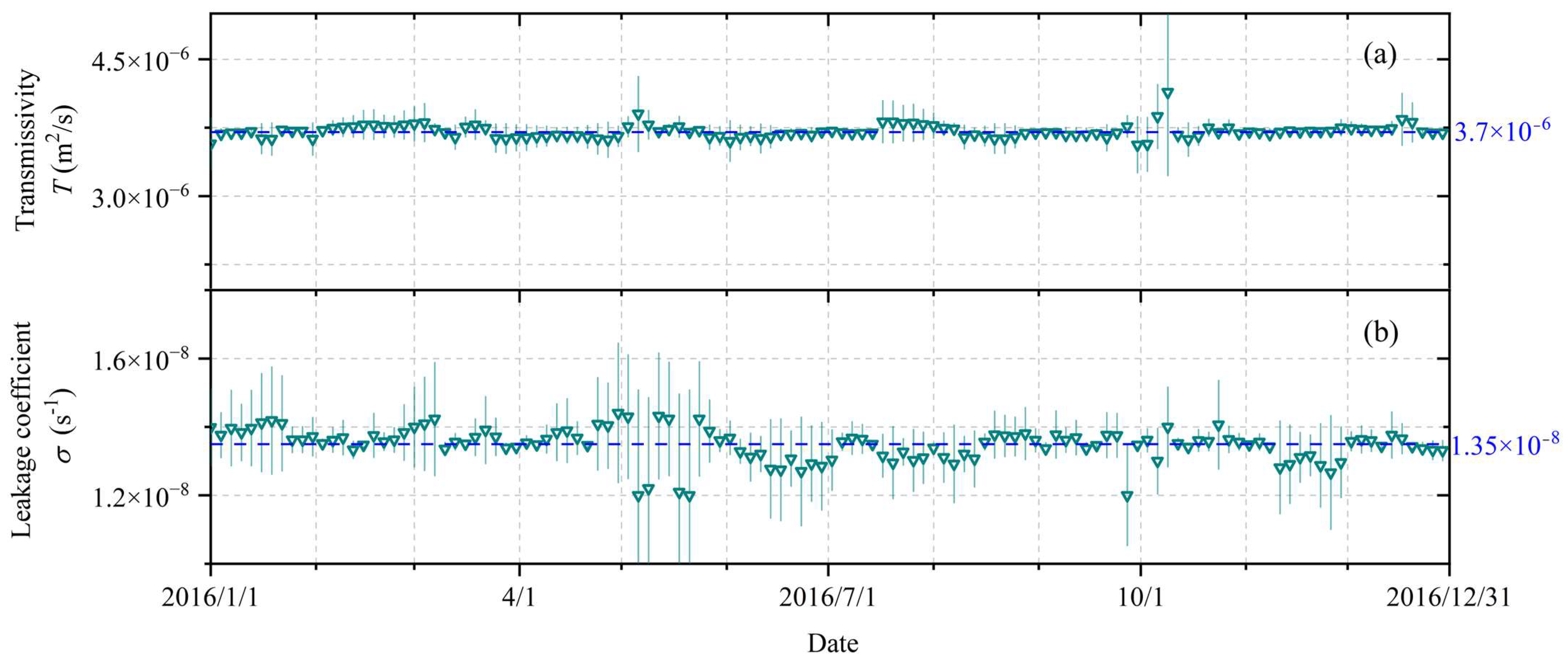
| Sun et al.’s method cited | 6.88 × 10⁻⁵ | 3.76 × 10⁻⁶ | 1.38 × 10⁻⁸ |
| This paper | 6.88 × 10⁻⁵ | 3.7 × 10⁻⁶ | 1.35 × 10⁻⁸ |
Disclaimer/Publisher’s Note: The statements, opinions and data contained in all publications are solely those of the individual author(s) and contributor(s) and not of MDPI and/or the editor(s). MDPI and/or the editor(s) disclaim responsibility for any injury to people or property resulting from any ideas, methods, instructions or products referred to in the content. |
© 2024 by the authors. Licensee MDPI, Basel, Switzerland. This article is an open access article distributed under the terms and conditions of the Creative Commons Attribution (CC BY) license (https://creativecommons.org/licenses/by/4.0/).
Share and Cite
Qiao, P.; Lan, S.; Gu, H.; Mao, Z. Using the Periodic Dynamics of Well Water Levels to Estimate Time Series Changes in Aquifer Parameters. Water 2024, 16, 1119. https://doi.org/10.3390/w16081119
Qiao P, Lan S, Gu H, Mao Z. Using the Periodic Dynamics of Well Water Levels to Estimate Time Series Changes in Aquifer Parameters. Water. 2024; 16(8):1119. https://doi.org/10.3390/w16081119
Chicago/Turabian StyleQiao, Peng, Shuangshuang Lan, Hongbiao Gu, and Zhengtan Mao. 2024. "Using the Periodic Dynamics of Well Water Levels to Estimate Time Series Changes in Aquifer Parameters" Water 16, no. 8: 1119. https://doi.org/10.3390/w16081119
APA StyleQiao, P., Lan, S., Gu, H., & Mao, Z. (2024). Using the Periodic Dynamics of Well Water Levels to Estimate Time Series Changes in Aquifer Parameters. Water, 16(8), 1119. https://doi.org/10.3390/w16081119